Continual Learning in Linear Classification on Separable Data

Itay Evron    Edward Moroshko    Gon Buzaglo    Maroun Khriesh    Badea Marjieh    Nathan Srebro    Daniel Soudry
Abstract

We analyze continual learning on a sequence of separable linear classification tasks with binary labels. We show theoretically that learning with weak regularization reduces to solving a sequential max-margin problem, corresponding to a special case of the Projection Onto Convex Sets (POCS) framework. We then develop upper bounds on the forgetting and other quantities of interest under various settings with recurring tasks, including cyclic and random orderings of tasks. We discuss several practical implications to popular training practices like regularization scheduling and weighting. We point out several theoretical differences between our continual classification setting and a recently studied continual regression setting.

Continual learning, Linear classification, Catastrophic forgetting

Figure 1: Illustrating our setting from Section 2 and the Sequential Max-Margin dynamics from Scheme 2 in Section 3.

Refer to caption

(a) A $2$-dimensional task with two samples (one positive and one negative). Each sample $(\mathbf{x},y)$ induces a constraint to a halfspace $y\mathbf{w}^{\top}\mathbf{x}\geq 1$. The task’s feasible set $\mathcal{W}_{1}$ is defined as the intersection of these two halfspaces, and is thus an affine polyhedral cone.

Refer to caption

(b) Two tasks, the first having two samples and the second having a single sample. The intersection of $\mathcal{W}_{1}$ and $\mathcal{W}_{2}$ defines the offline feasible set $\mathcal{W}^{\star}$, in which all samples of all tasks are correctly classified with a margin of at least $1$. Notice the min-norm offline solution $\mathbf{w}^{\star}\in\mathcal{W}^{\star}$.

Refer to caption

(c) Learning the 1st task projects ${\mathbf{w}_{0}\!=\!\mathbf{0}_{D}}$ onto $\mathcal{W}_{1}$. The obtained iterate ${\mathbf{w}_{1}={\mathbf{P}}_{1}(\mathbf{w}_{0})}$ is the max-margin solution of the 1st task. Then, learning the 2nd task, projects $\mathbf{w}_{1}$ onto $\mathcal{W}_{2}$ to obtain (in this case) an offline solution ${\mathbf{w}_{2}={\mathbf{P}}_{2}(\mathbf{w}_{1})\in\mathcal{W}^{\star}\subset\mathcal{W}_{2}}$. Notably, $\mathbf{w}_{2}$ is not the min-norm $\mathbf{w}^{\star}$ (Section 4.3).

1 Introduction

Continual learning deals with learning settings where distributions, or tasks, change over time, breaking traditional i.i.d. assumptions. While models trained sequentially are expected to accumulate knowledge and improve over time, practically they suffer from catastrophic forgetting (McCloskey & Cohen, 1989; Goodfellow et al., 2013), i.e., their performance on previously seen tasks deteriorates over time.

Much research in continual learning has focused on heuristic approaches to remedying forgetting. Recent approaches achieve impressive empirical performance, but often require storing examples from previous tasks (e.g., Robins (1995); Rolnick et al. (2019)), iteratively expanding the learned models (e.g., Yoon et al. (2018)), or lessening the plasticity of these models and harming their performance on new tasks (e.g., Kirkpatrick et al. (2017)).

We theoretically study the continual learning of a linear classification model on separable data with binary classes. Even though this is a fundamental setup to consider, there are still very few analytic results on it, since most of the continual learning theory thus far has focused on regression settings (e.g., Bennani et al. (2020); Doan et al. (2021); Asanuma et al. (2021); Lee et al. (2021); Evron et al. (2022); Goldfarb & Hand (2023); Li et al. (2023)). Even in the broader deep learning scope, theoreticians often start from very simple models and use them to gain insight into phenomena arising in more practical models (e.g., Belkin et al. (2018); Woodworth et al. (2020)).

Our paper reveals a surprising algorithmic bias of linear classifiers trained continually to minimize the exponential loss on separable data with weak regularization. Specifically, we prove that the weights converge in the same direction as the iterates of a Sequential Max-Margin scheme. This creates a bridge between the popular regularization methods for continual learning (Kirkpatrick et al., 2017; Zenke et al., 2017) and the well-studied POCS framework – Projections Onto Convex Sets (also known as the convex feasibility problem or successive projections).

Our results complement those of a recent paper (Evron et al., 2022) that analyzed the worst-case performance of continual linear regression. That paper showed that continually learning linear regression tasks with vanilla SGD, implicitly performs sequential projections onto closed subspaces, and connected that regime to the area of Alternating Projections (Von Neumann, 1949; Halperin, 1962). In our paper, we draw comparisons between our continual classification setting and their continual regression setting (summarized in App. A). We point out inherent differences between these two settings, emphasizing the need for a proper and thorough analytical understanding dedicated to continual classification settings.

Our Contributions

Our analysis reveals the following:

  • Explicit regularization methods for continual learning of linear classification models are linked to the framework of Projections Onto Convex Sets (POCS).

  • Each learned task brings the learner closer to an “offline” feasible solution solving all tasks. However, there exist task sequences for which the learner stays arbitrarily far from offline feasibility, even after infinitely many tasks.

  • When tasks recur cyclically or randomly, the learner converges to an offline solution with linear rates.

  • If we converge to an offline solution, it may not be the minimum-norm solution (in contrast to continual regression), but it still needs to be $2$-optimal (minimal).

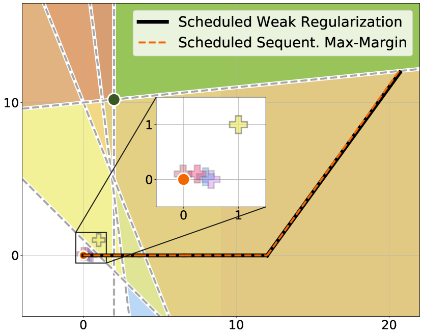
  • Scheduling the regularization strength endangers convergence to an offline solution and optimality guarantees.

  • Using popular regularization weighting schemes based on Fisher-information matrices, does not necessarily prevent forgetting (in contrast to continual regression).

  • Early stopping (without regularization) does not yield the same solutions as weak regularization (unlike in stationary settings with a single task).

2 Setting

We consider $T\geq 2$ binary classification tasks. Each task $m=1,\dots,T$ is defined by a dataset $S_{m}$ consisting of tuples of $D$-dimensional samples and their binary labels, i.e., each tuple is $(\mathbf{x},y)\!\in\!{\,\mathbb{R}^{D}\!\times\!\left\{-1,+1\right\}\,}$, for a finite $D$.

Notation.

Throughout the paper, we denote the (isotropic) Euclidean norm of vectors by $\left\|{\mathbf{v}}\right\|$, and the weighted norm by $\left\|{\mathbf{v}}\right\|_{\mathbf{B}}\triangleq\mathbf{v}^{\top}\mathbf{B}\mathbf{v}$, for some $\mathbf{B}\succ\mathbf{0}_{D\times D}$. We denote the set of natural numbers starting from $1$ by ${\mathbb{N}^{+}\triangleq\mathbb{N}\setminus\{0\}}$ and the natural numbers from $1$ to $n$ by $\left[{n}\right]$. We define the distance of a vector $\mathbf{w}\in\mathbb{R}^{D}$ from a closed set $\mathcal{C}\subseteq\mathbb{R}^{D}$ as ${{d}(\mathbf{w},\mathcal{C})\triangleq\min_{\mathbf{v}\in\mathcal{C}}\left\|{\mathbf{w}-\mathbf{v}}\right\|}$. Finally, we denote the maximal norm of any data point by ${R\triangleq\max_{m\in\left[{T}\right]}\max_{(\mathbf{x},y)\in S_{m}}\left\|{\mathbf{x}}\right\|}$.

Our main assumption in this paper is that the tasks are jointly-separable, i.e., they can be perfectly fitted simultaneously, as in “offline” non-continual settings. This can be formally stated as follows.

Assumption 2.1 (Separability).

Each task $m\in\left[{T}\right]$ is separable, i.e., it has a non-empty feasible set defined as

$$\mathcal{W}_{m}\,\!\triangleq\!\,\left\{\mathbf{w}\!\in\!\mathbb{R}^{D}\mid y\mathbf{w}^{\top}\mathbf{x}\geq 1,~{}\forall(\mathbf{x},y)\in S_{m}\right\}\,.$$

Moreover, the $T$ tasks are jointly-separable — there exists a non-empty offline feasible set:

$$\mathcal{W}^{\star}\,\!\triangleq\!\,\mathcal{W}_{1}\cap\dots\cap\mathcal{W}_{T}\neq\emptyset\,.$$

A similar assumption was made in the continual regression setting (Evron et al., 2022). It is a reasonable assumption in overparameterized regimes, where feasible offline solutions often do exist. Practically, this is commonly the case in modern deep networks. Theoretically, with sufficient overparameterization (Du et al., 2019) or high enough margin (Ji & Telgarsky, 2020), it is often easy to converge to a zero-loss solution.


To facilitate our results and discussions, we specifically define the minimum-norm offline solution. This solution is traditionally linked to good generalization.

Definition 2.2 (Minimum-norm offline solution).

We denote the offline solution with the minimal norm by

$\displaystyle\begin{aligned} \mathbf{w}^{\star}\triangleq{\operatorname*{argmin}}_{\mathbf{w}\in\mathcal{W}^{\star}}\left\|{\mathbf{w}}\right\|\,.\end{aligned}$

Figures 1(a) and 1(b) illustrate our definitions. Notice how both the feasible set $\mathcal{W}_{m}$ of each task and the offline feasible set $\mathcal{W}^{\star}$ are closed, convex, and affine polyhedral cones.

3 Algorithmic Bias in Regularization Methods

Regularization methods are highly influential in continual learning (Kirkpatrick et al., 2017; Zenke et al., 2017; Aljundi et al., 2018). In this section, we propose a novel analysis for such methods on separable datasets in the spirit of theoretical work on algorithmic biases outside the scope of continual learning. Concretely, we discover that weakly-regularized models, trained sequentially to minimize the exponential loss,111 It should be possible to extend our results to other losses with exponential tails, e.g., cross-entropy, as has been done in previous theoretical works on stationary settings (Soudry et al., 2018). converge in direction to the iterates of a sequential projection scheme.

Specifically, we study Scheme 1, in which the learner sequentially sees one task (out of $T$) at a time, for $k$ iterations ($k\!>\!T$ implies repetitions). Starting from $\mathbf{w}_{0}^{(\lambda)}\!\!=\!\!\mathbf{0}_{D}$, at each iteration $t\!\in\!\left[{k}\right]$, the learner minimizes the exponential loss of the current task’s dataset $S_{t}$, while biasing towards the previous task’s solution $\mathbf{w}_{t-1}^{(\lambda)}$ using the Euclidean norm. The regularization strength is determined by a sequence of (possibly constant) positive scalars $\lambda_{1},.\hskip 0.8pt\!.\hskip 0.8pt\!.,\lambda_{k}\!>\!0$. The norms are possibly weighted by a sequence of positive-definite matrices $\mathbf{B}_{1},.\hskip 0.8pt\!.\hskip 0.8pt\!.,\mathbf{B}_{k}\succ\mathbf{0}_{D\times D}$.

Scheme 1 Regularized Continual Learning
  Initialization: $\mathbf{w}_{0}^{(\lambda)}=\mathbf{0}_{D}$
  Iterative update for each task $t\in[k]$:
$\displaystyle\mathbf{w}_{t}^{(\lambda)}\!=\operatorname*{argmin}_{\mathbf{w}\in\mathbb{R}^{D}}\!\!{\sum_{(\mathbf{x},y)\in S_{t}}\!\!\!e^{-y\mathbf{w}^{\top}\mathbf{x}}+\frac{\lambda_{t}}{2}\left\|{\mathbf{w}\!-\!\mathbf{w}_{t-1}^{(\lambda)}}\right\|^{2}_{\mathbf{B}_{t}}}$ (1)

To clarify, each of the $k$ iterations corresponds to learning a whole task (to convergence), and not to performing a single gradient step.

As a start, we first focus on constant strengths $\lambda\!>\!0$ and on “vanilla” L$2$ regularization, i.e., $\mathbf{B}_{1}=.\hskip 0.8pt\!.\hskip 0.8pt\!.=\mathbf{B}_{k}=\mathbf{I}$. Vanilla L$2$ regularization has recently been shown to be competitive with more popular norm-weighting schemes like EWC (Lubana et al., 2022; Smith et al., 2023). We address the more complicated setups in Section 5.

For an arbitrary $\lambda$, the objective in Eq. (1) is hard to analyze, even for the first task, where the regularization term reduces to the traditional unbiased term $\left\|{\mathbf{w}}\right\|^{2}$. Previous works were still able to perform non-trivial analysis by examining the weakly-regularized case, i.e., in the limit of $\lambda\to 0$ (e.g., for linear models (Rosset et al., 2004) or homogeneous neural networks (Wei et al., 2019)).

Under our continual setting, we also take this approach and analyze the weakly-regularized model. This enables us to gain analytical insights into regularization methods for continual learning. We establish an equivalence between the weakly-regularized Scheme 1 and the following Sequential Max-Margin Scheme 2, and propose novel perspectives and techniques for analyzing regularization methods.

Scheme 2 Sequential Max-Margin
  Initialization: $\mathbf{w}_{0}=\mathbf{0}_{D}$
  Iterative update for each task $t\in[k]$:
$\displaystyle\mathbf{w}_{t}={\mathbf{P}}_{t}\left({\mathbf{w}_{t-1}}\right)\triangleq\operatorname*{argmin}_{\mathbf{w}\in\mathbb{R}^{D}}\enskip$ $\displaystyle\!\left\|{\mathbf{w}-{\mathbf{w}}_{t-1}}\right\|^{2}$ (2)
s.t. $\displaystyle\,y\mathbf{w}^{\top}\mathbf{x}\!\geq\!1,\,\forall(\mathbf{x},y)\!\in\!S_{t}$

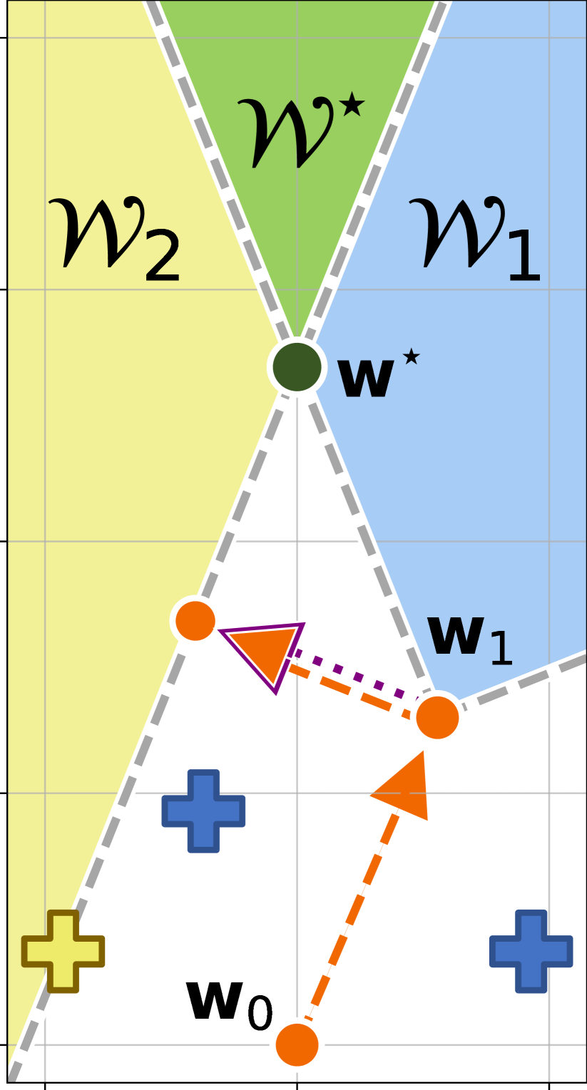
We are now ready to state our fundamental result, showing that the regularized continual iterates $({\mathbf{w}_{t}^{(\lambda)}})$ of Scheme 1 converge in direction to the Sequential Max-Margin iterates $\left({\mathbf{w}_{t}}\right)=({{\mathbf{P}}_{t}\left({\mathbf{w}_{t-1}}\right)})$ of Scheme 2, obtained by successive projections onto closed convex sets, as depicted in Figure 1(c).

Theorem 3.1 (Weakly-regularized Continual Learning converges to Sequential Max-Margin).

Let $\lambda_{t}\!=\!\lambda\!>\!0$, and $\mathbf{B}_{t}\!=\!\mathbf{I}$, $\forall t\!\in\!\left[{k}\right]$. Then, for almost all separable datasets,222 This holds w.p. $1$ for separable datasets (Assumption 2.1) sampled from any absolutely continuous distribution. It also holds even when the datasets are separable but not jointly-separable. in the limit of $\lambda\!\to\!0$, it holds that $\mathbf{w}_{t}^{(\lambda)}\to{\ln\left({\tfrac{1}{\lambda}}\right)\mathbf{w}_{t}}$ with a residual of $\|{\mathbf{w}_{t}^{(\lambda)}\!-{\ln\left({\tfrac{1}{\lambda}}\right)\mathbf{w}_{t}}}\|=\mathcal{O}\left({t\ln\ln\left({\tfrac{1}{\lambda}}\right)}\right)$. As a result, at any iteration $t=o\left({\frac{\ln\left({\nicefrac{{1}}{{\lambda}}}\right)}{\ln\ln\left({\nicefrac{{1}}{{\lambda}}}\right)}}\right)$, we get

limλ0𝐰t(λ)𝐰t(λ)=𝐰t𝐰t.subscript𝜆0superscriptsubscript𝐰𝑡𝜆normsuperscriptsubscript𝐰𝑡𝜆subscript𝐰𝑡normsubscript𝐰𝑡\lim_{\lambda\to 0}\frac{\mathbf{w}_{t}^{(\lambda)}}{\|{\mathbf{w}_{t}^{(\lambda)}}\|}=\frac{\mathbf{w}_{t}}{\|{\mathbf{w}_{t}}\|}\,.

In Appendix B, we prove this theorem. There, we also discuss the limitations of our analysis (Appendix B.3) and identify aspects where it can be improved.

Remark 3.2 (Important differences from existing analysis).

Existing works (e.g., Rosset et al. (2004)) analyzed weakly-regularized models with an unbiased regularizer $\left\|{\mathbf{w}}\right\|_{p}^{p}$. This allowed them to concentrate on the limit margin which implies convergence in direction. However, we show that to analyze the continual regularizer in Eq. (1), one must also take into account the scale of the solutions $(\mathbf{w}_{t}^{(\lambda)})$. Therefore, we analyze both the scale and the direction of weakly-regularized solutions, requiring more refined techniques.

4 Sequential Max-Margin Projections

Now, we turn to exploit the connection we have established between the weakly-regularized continual Scheme 1 and the Sequential Max-Margin Scheme 2. Using tools from existing literature on Projections Onto Convex Sets (POCS), we gain valuable insights into the dynamics of training models continually. Specifically, we derive optimality guarantees and convergence bounds in several interesting settings.

4.1 Quantities of Interest

We have three quantities of interest. While the first two are widely used in the POCS literature, the latter is specific to our continual classification setting.

Definition 4.1 (Quantities of interest).

Let $\mathbf{w}_{t}\in\mathbb{R}^{D}$ be the $t$th iterate, obtained while continually learning $T$ jointly-separable tasks. The following quantities are of interest:

  1. 1.

    Distance to the offline feasible set: ${d}\!\left({\mathbf{w}_{t},\mathcal{W}^{\star}}\right)$

  2. 2.

    Maximum dist. to any feasible set: $\displaystyle\max_{m\in\left[{T}\right]}\!{d}\!\left({\mathbf{w}_{t},\mathcal{W}_{m}}\right)$

  3. 3.

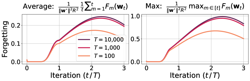
    Forgetting: We define the forgetting of a previously-seen task ${m\in\left[{t}\right]}$ as the maximal squared hinge loss on any sample $(\mathbf{x},y)$ of the task. More formally,

    $$F_{m}(\mathbf{w}_{t})\triangleq{\max}_{(\mathbf{x},y)\in S_{m}}\!\left(\max\left\{0,\,1-y\mathbf{w}_{t}^{\top}\mathbf{x}\right\}\right)^{2}\,.$$

    Throughout our paper, we analyze both the maximal and the average forgetting, i.e., $\max_{m\in\left[{t}\right]}F_{m}(\mathbf{w}_{t})$ and $\tfrac{1}{t}\sum_{m=1}^{t}F_{m}(\mathbf{w}_{t})$.

Explaining our forgetting.

Previous works on continual linear regression defined forgetting using the MSE on previously-seen tasks, i.e., ${\forall m<t\!:~{}F_{m}(\mathbf{w}_{t})=\tfrac{1}{\left|{S_{m}}\right|}\sum_{(\mathbf{x},y)\in S_{m}}\left({\mathbf{w}_{t}^{\top}\mathbf{x}-y}\right)^{2}}$ (e.g., Doan et al. (2021); Evron et al. (2022)). Then, lower forgetting implies better training loss on previous tasks.

In continual linear classification, hinge losses capture similar properties. First, per our definitions, immediately after learning the $m$th task, the forgetting on it is 00, since $\forall\mathbf{v}\!\in\!\mathbb{R}^{D}\!:{\mathbf{P}}_{m}(\mathbf{v})\!\in\!\mathcal{W}_{m}$ and $\forall\mathbf{u}\!\in\!\mathcal{W}_{m}\!:F_{m}(\mathbf{u})=0$. Moreover, a lower forgetting implies better training margins and generalization performance on previous tasks. Since the squared hinge loss is a surrogate for the 0-1 loss, $F_{m}\!\left({\mathbf{w}_{t}}\right)\!<\!1$ implies no prediction errors on the $m$th task.

Remark 4.2 (Forgetting vs. Regret).

Forgetting is different from the regret used to analyze online learning algorithms (Crammer et al., 2006; Shalev-Shwartz et al., 2012; Hoi et al., 2021). Forgetting quantifies the degradation on previous tasks in hindsight, while regret cumulatively captures the ability to predict future datapoints (or tasks).

A favorable property of the quantities we defined, is that they bound each other.

Lemma 4.3 (Connecting quantities).

Recall our definition of ${R\triangleq\max_{m\in\left[{T}\right]}\max_{(\mathbf{x},y)\in S_{m}}\!\!\left\|{\mathbf{x}}\right\|}$. The quantities of Def. 4.1 are related as follows, $\forall\mathbf{w}\!\in\!\mathbb{R}^{D},\,m\!\in\!\left[{T}\right]$:

$\displaystyle F_{m}(\mathbf{w})\leq{d}^{2}(\mathbf{w},\mathcal{W}_{m})\!\!\max_{(\mathbf{x},y)\in S_{m}}\!\!\!\!\|{\mathbf{x}}\|^{2}\leq{d}^{2}(\mathbf{w},\mathcal{W}^{\star})R^{2}.$

Moreover, for the Sequential Max-Margin iterates (𝐰t)subscript𝐰𝑡(\mathbf{w}_{t}) of Scheme 2, all quantities are upper bounded by the “problem complexity”, i.e., d2(𝐰t,𝒲)R2𝐰2R2superscript𝑑2subscript𝐰𝑡superscript𝒲superscript𝑅2superscriptnormsuperscript𝐰2superscript𝑅2{d}^{2}(\mathbf{w}_{t},\mathcal{W}^{\star})R^{2}\leq\left\|{\mathbf{w}^{\star}}\right\|^{2}\!R^{2}.

The proof is given in Appendix C.

Remark 4.4 (Problem complexity).

Many of our bounds use $\left\|{\mathbf{w}^{\star}}\right\|^{2}\!R^{2}$, which can be seen as the problem complexity due to its links to sample complexities (Novikoff, 1962). Moreover, Assumption 2.1, implies that $\left\|{\mathbf{w}^{\star}}\right\|^{2}\!R^{2}\geq 1$.

The following is a known useful result from the POCS literature (e.g., Lemma 3 in Gubin et al. (1967)).

Lemma 4.5 (Monotonicity of distances to offline feasibility).

Distances from the Sequential Max-Margin iterates of Scheme 2 to the offline feasible set are non-increasing, i.e.,

$${d}(\mathbf{w}_{t},\mathcal{W}^{\star})\leq{d}(\mathbf{w}_{t-1},\mathcal{W}^{\star}),~{}\,\forall t\in\left[{k}\right]\,.$$
Question

An immediate question arises from Lemma 4.5: when learning infinite jointly-separable tasks ($k=T\!\to\!\infty$), must we converge to the offline feasible set $\mathcal{W}^{\star}$? Next, we answer this question in the negative.

4.2 Adversarial Construction: Maximal Forgetting

Example 1 (Adversarial construction).

We present a construction of task sequences that seemingly exhibit arbitrarily bad continual performance. Even after seeing $k=T\to\infty$ jointly-separable tasks, the learner stays afar from the offline feasible set $\mathcal{W}^{\star}$, and the forgetting of previously-seen tasks is maximal. The learner fails to successfully accumulate experience. See further details in Appendix C.1.

(a) Our construction with $T\!=\!20$ tasks in $D\!=\!3$. Datapoints (each defining a task) have a norm of $R\!=\!1$ and are spread uniformly on a plane, slightly elevated above the $xy$-plane. It holds that $\left\|{\mathbf{w}^{\star}}\right\|\!=\!10$. As $T\!\to\!\infty$, angles between consecutive tasks and applied projections, get smaller.
Refer to caption
Refer to caption
(b) The average and maximum forgetting for the adversarial construction for an increasing number of tasks $T$. Recall that the maximum forgetting lower bounds the distance to the offline feasible set (Lemma 4.3). Notably, after learning $T\to\infty$ jointly separable tasks, the quantities do not decay but seemingly become arbitrarily bad (close to $\left\|{\mathbf{w}^{\star}}\right\|^{2}\!R^{2}$) at some point of learning.
Figure 2: Illustrations of our adversarial construction.
Remark 4.6 (Order of limits).

Our paper analyzes the continual learning of $T$ tasks for $k$ iterations, possibly taking ${k\!\to\!\infty}$ (e.g., by repeating tasks). We take $\lambda\!\to\!0$ after fixing the number of iterations $k$. As a result, limit iterates hold

$$\frac{\mathbf{w}_{\infty}}{\|{\mathbf{w}_{\infty}}\|}\triangleq\lim_{k\to\infty}\frac{\mathbf{w}_{k}}{\|{\mathbf{w}_{k}}\|}=\lim_{k\to\infty}\lim_{\lambda\to 0}\frac{\mathbf{w}_{k}^{(\lambda)}}{\|{\mathbf{w}_{k}^{(\lambda)}}\|}\,.$$

4.3 Convergence to the Minimum-Norm Solution

When solving feasibility problems for classification (e.g., in hard-margin SVM), the minimum-norm solution is also the max-margin solution. In turn, max-margin solutions are theoretically linked to better generalization performance.

In realizable continual linear regression (or generally, in alternating projections onto closed subspaces), it is known that if iterates converge to an offline (or globally feasible) solution, then that solution must be the closest to $\mathbf{w}_{0}$, i.e., have a minimum norm (Evron et al., 2022; Halperin, 1962).

In contrast, in separable continual linear classification settings like ours (or generally, in projections onto closed convex sets), there is no such guarantee and we can converge to a suboptimal offline solution, as depicted in Figure 1(c).

Nevertheless, the following optimality guarantee does hold.

Theorem 4.7 (Optimality guarantee).

Any iterate $\mathbf{w}_{t}$ obtained by Scheme 2 holds $\left\|{\mathbf{w}_{t}}\right\|\leq 2\left\|{\mathbf{w}^{\star}}\right\|$, where $\mathbf{w}^{\star}$ is the minimum-norm offline solution (Def. 2.2).

If additionally, 𝐰tsubscript𝐰𝑡\mathbf{w}_{t} is “offline”-feasible, i.e., 𝐰t𝒲subscript𝐰𝑡superscript𝒲\mathbf{w}_{t}\in\mathcal{W}^{\star}, then

𝐰𝐰t2𝐰.normsuperscript𝐰normsubscript𝐰𝑡2normsuperscript𝐰\left\|{\mathbf{w}^{\star}}\right\|\leq\left\|{\mathbf{w}_{t}}\right\|\leq 2\left\|{\mathbf{w}^{\star}}\right\|\,.

The proof is given in Appendix C.2. Further comparisons to continual regression are drawn in Appendix A.

4.4 Recurring Tasks

Naturally, in many practical continual problems, certain concepts and experiences recur at different tasks (e.g., environments of an autonomous vehicle, levels of a computer game, trends of a search engine, etc.).

Several recent papers have observed empirically that task repetitions mitigate catastrophic forgetting in continual learning (Stojanov et al., 2019; Cossu et al., 2022), even when training is performed with vanilla SGD, without any forgetting-preventing method (Lesort et al., 2022).

In this section, we analytically study the influence of repetitions. To accomplish this, we leverage the connection that we have established between continual learning and successive projection algorithms for convex feasibility problems. Importantly, we do not propose repetitions as a training method but rather aim to understand their effects on continual learning from a projection perspective.

The results of this section are summarized in Table 1.

Table 1: Summary of our upper bounds for recurring orderings (Section 4.4). Upper bounds of random orderings apply to the expectations.
Ordering Iterate type $\displaystyle\tfrac{1}{\|{\mathbf{w}^{\star}}\|^{2}R^{2}}{\max}_{m\in\left[{T}\right]}F_{m}(\mathbf{w}_{k})$ $\displaystyle\tfrac{1}{\|{\mathbf{w}^{\star}}\|^{2}}{\max}_{m\in\left[{T}\right]}{d}^{2}\left({\mathbf{w}_{k},\mathcal{W}_{m}}\right)$ $\displaystyle\tfrac{1}{\|{\mathbf{w}^{\star}}\|^{2}}{d}^{2}\left({\mathbf{w}_{k},\mathcal{W}^{\star}}\right)$
Cyclic Last ($T=2$) $\displaystyle\min\bigg{\{}\frac{1}{k+1},\,\,\,\,\,\,\,\,\,\,\,\,\,\,\,\exp\!\Big{(}{-\frac{k}{4\|{\mathbf{w}^{\star}}\|^{2}R^{2}}}\Big{)}\Big{\}}$ $\displaystyle\exp\!\Big{(}{-\frac{k}{4\|{\mathbf{w}^{\star}}\|^{2}R^{2}}}\Big{)}$
Last ($T\geq 3$) $\displaystyle\min\bigg{\{}\,\frac{2T^{2}}{\sqrt{k}},\,\,\,4\exp\!\Big{(}{-\frac{k}{16T^{2}\|{\mathbf{w}^{\star}}\|^{2}R^{2}}}\Big{)}\Big{\}}$ $\displaystyle\exp\!\Big{(}{-\frac{k}{16T^{2}\|{\mathbf{w}^{\star}}\|^{2}R^{2}}}\Big{)}$
Average ($T\geq 2$) ${T^{2}}/{k}$
Random Last $\displaystyle\exp\!\Big{(}{-\frac{k}{4T\|{\mathbf{w}^{\star}}\|^{2}R^{2}}}\Big{)}$ $\displaystyle\exp\!\Big{(}{-\frac{k}{4T\|{\mathbf{w}^{\star}}\|^{2}R^{2}}}\Big{)}$
(i.i.d.) Average ${T}/{k}$
Recurring tasks vs. Batch learning

The recurring tasks setting should not be confused with standard batch training (i.e., by regarding each task as a batch). While in batch training, a single gradient-descent step is made for each batch, in our continual learning setting (Scheme 1) each task is solved completely (to separation).

The following is a key lemma in our paper. Much of the research on POCS has focused on defining and applying linear regularity conditions, under which iterates $(\mathbf{w}_{t})$ converge linearly (like $c^{t}$ for some $c\!\in\!\left[0,1\right)$) to the feasible sets’ intersection $\mathcal{W}^{\star}$ (e.g., Bauschke & Borwein (1993)). In realizable continual linear regression, Evron et al. (2022) showed that no such regularity holds, and while their forgetting, i.e., ${F_{m}(\mathbf{w}_{t})\triangleq{d}^{2}(\mathbf{w}_{t},\mathcal{W}_{m}),~{}\forall m\!\in\!\left[{T}\right]}$, is upper bounded universally, no universal bounds can be derived for ${d}^{2}(\mathbf{w}_{t},\mathcal{W}^{\star})$ even when $\left\|{\mathbf{w}^{\star}}\right\|$ and $R$ are bounded. In contrast, we prove that in separable continual linear classification, linear regularity does hold and nontrivial bounds can be derived for ${d}^{2}(\mathbf{w}_{t},\mathcal{W}^{\star})$.

Lemma 4.8 (Linear regularity of Sequential Max-Margin).

At the $t$th iteration, the distance to the offline feasible set is tied to the distance to the farthest feasible set of any specific task. Specifically, it holds that $\forall t\!\in\!\mathbb{N}^{+}$,

$\displaystyle{d}^{2}\!\left({\mathbf{w}_{t},\mathcal{W}^{\star}}\right)\leq 4\,\|{\mathbf{w}^{\star}}\|^{2}R^{2}\max_{m\in\left[{T}\right]}{d}^{2}\big{(}{\mathbf{w}_{t},\mathcal{W}_{m}}\big{)}\,.$

The proofs for this section are given in Appendix D.

So far we assumed that at iteration $t$, the learner solves a task, i.e., a dataset $S_{t}$ (out of $T$ possible datasets), corresponding to a projection ${\mathbf{P}}_{t}$. To facilitate our next results for cases where tasks recur, we now define task ordering functions.

Definition 4.9 (Task ordering).

A task ordering is a function

$$\tau:~{}\mathbb{N}^{+}\to\left[{T}\right]$$

that maps an iteration to a learning task.

4.4.1 Cyclic Ordering

Mathematically, when analyzing successive projections (like in our Scheme 2), it is common to first study a cyclic setting, where the projections form a clearer (cyclic) operator. This setting has been at the center of focus in many theoretical papers (e.g., Agmon (1954); Halperin (1962); Deutsch & Hundal (2006a); Borwein et al. (2014); Evron et al. (2022)).

Practically, in continual learning, cyclic orderings are indeed less flexible. However, we believe that they do emerge naturally in real-world scenarios. For instance, virtual assistants support the recurring daily routines of their customers and should be able to continue learning from new experiences.

Definition 4.10 (Cyclic task ordering).

A cyclic ordering over $T$ tasks is defined as

$$\tau(t)\triangleq 1+\left({\left({t-1}\right)\bmod T}\right),\enskip~{}\forall t\in\mathbb{N}^{+}\,,$$

and induces a cyclic operator, in the sense that

$$\mathbf{w}_{nT}=\left({{\mathbf{P}}_{\tau(nT)}\circ\hskip 0.6pt\cdotp\!\hskip 0.6pt\cdotp\!\hskip 0.6pt\cdotp\!\hskip 0.6pt\circ{\mathbf{P}}_{\tau(1)}}\right)\!(\mathbf{w}_{0})=({\mathbf{P}}_{T}\circ\hskip 0.6pt\cdotp\!\hskip 0.6pt\cdotp\!\hskip 0.6pt\cdotp\!\hskip 0.6pt\circ{\mathbf{P}}_{1})^{n}(\mathbf{w}_{0}).$$

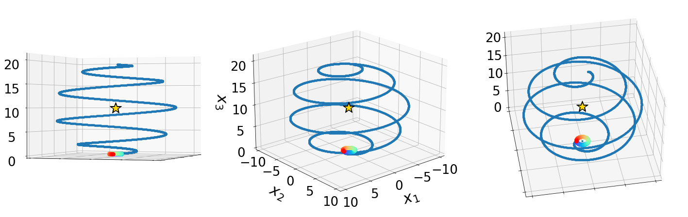
We illustrate such orderings in the following Figure 3.

Refer to caption

Figure 3: A cyclic setting with two tasks. Each time we solve a task, we project the previous iterate onto its corresponding convex set.

Using the linear regularity from Lemma 4.8, we prove linear convergence results for cyclic orderings. Our proofs use tools and results from existing POCS literature.

Lemma 4.11 (Limit guarantees for cyclic orderings).

Under a cyclic ordering (and the separability assumption 2.1), the iterates converge to a 2-optimal ${\mathbf{w}_{\infty}\in\mathcal{W}^{\star}}$. That is,

limkd(𝐰k,𝒲)=0,𝐰𝐰2𝐰.formulae-sequencesubscript𝑘𝑑subscript𝐰𝑘superscript𝒲0normsuperscript𝐰normsubscript𝐰2normsuperscript𝐰\lim_{k\to\infty}{d}(\mathbf{w}_{k},\mathcal{W}^{\star})=0,~{}~{}~{}\left\|{\mathbf{w}^{\star}}\right\|\leq\left\|{\mathbf{w}_{\infty}}\right\|\leq 2\left\|{\mathbf{w}^{\star}}\right\|\,.

The proofs for this section are given in Appendix D.3.


Theorem 4.12 (Linear rates for cyclic orderings).

For ${T\geq 2}$ jointly-separable tasks learned cyclically, after ${k\!=\!nT}$ iterations ($n$ cycles), our quantities of interest (Def. 4.1) converge linearly as

$\displaystyle\underbrace{\max_{m\in\left[{T}\right]}F_{m}(\mathbf{w}_{k})}_{\begin{subarray}{c}\text{Maximum forgetting}\end{subarray}}$ $\displaystyle\leq\underbrace{\max_{m\in\left[{T}\right]}{d}^{2\!}\left({\mathbf{w}_{k},\mathcal{W}_{m}}\right)}_{\begin{subarray}{c}\text{Max.~{}dist.~{}to any feasible set}\end{subarray}}R^{2}\leq$
$\displaystyle\leq\underbrace{{d}^{2\!}\left({\mathbf{w}_{k},\mathcal{W}^{\star}}\right)}_{\begin{subarray}{c}\text{Dist.~{}to}\\ \text{offline feasible set}\end{subarray}}R^{2}\leq g(k)\left\|{\mathbf{w}^{\star}}\right\|^{2}\!R^{2}\,,$

where

$$g(k)\triangleq\begin{cases}\enskip\,\exp\!\left({-\tfrac{k}{4\|{\mathbf{w}^{\star}}\|^{2}R^{2}}}\right)&T=2\\ 4\exp\!\left({-\tfrac{k}{16T^{2}\|{\mathbf{w}^{\star}}\|^{2}R^{2}}}\right)&T\geq 3\end{cases}$$

and $\left\|{\mathbf{w}^{\star}}\right\|^{2}\!R^{2}\!\geq\!1$ is the problem complexity (Rem. 4.4).

Detour: Universal rates for general cyclic Projections onto Convex Sets (POCS) settings.

We take a brief detour to derive universal bounds for general POCS settings, where problems do not necessarily hold regularity conditions like the ones in our Lemma 4.8. While cyclic POCS settings have been studied for decades (Agmon, 1954; Deutsch & Hundal, 2006a, b, 2008), most previous works either focused on settings with regularity assumptions or yielded problem-dependent rates that can be arbitrarily bad.

Our result below extends the universal results of a recent work that focused on closed subspaces only (Evron et al., 2022); and is also related to a recent work that considered closed convex sets as well, but dismissed the number of sets $T$ as $\mathcal{O}\left({1}\right)$ (Reich & Zalas, 2023).

Proposition 4.13 (Universal rates for general cyclic POCS).

Let $\mathcal{W}_{1},\dots,\mathcal{W}_{T}$ be closed convex sets with nonempty intersection $\mathcal{W}^{\star}$. Let $\mathbf{w}_{k}=({\mathbf{P}}_{T}\circ\cdots\circ{\mathbf{P}}_{1})^{n}(\mathbf{w}_{0})$ be the iterate after $k\!=\!nT$ iterations ($n$ cycles) of cyclic projections onto these convex sets. Then, the maximal distance to any (specific) convex set, is upper bounded universally as,

For T=2𝑇2T=2: maxm[T]d2(𝐰k,𝒲m)1k+1d2(𝐰0,𝒲),subscript𝑚delimited-[]𝑇superscript𝑑2subscript𝐰𝑘subscript𝒲𝑚1𝑘1superscript𝑑2subscript𝐰0superscript𝒲\displaystyle\max_{m\in\left[{T}\right]}{d}^{2\!}\left({\mathbf{w}_{k},\mathcal{W}_{m}}\right)\leq\frac{1}{k+1}\,{d}^{2\!}\left({\mathbf{w}_{0},\mathcal{W}^{\star}}\right)\,,
For T3𝑇3T\geq 3: maxm[T]d2(𝐰k,𝒲m)2T2kd2(𝐰0,𝒲).subscript𝑚delimited-[]𝑇superscript𝑑2subscript𝐰𝑘subscript𝒲𝑚2superscript𝑇2𝑘superscript𝑑2subscript𝐰0superscript𝒲\displaystyle\max_{m\in\left[{T}\right]}{d}^{2\!}\left({\mathbf{w}_{k},\mathcal{W}_{m}}\right)\leq\frac{2T^{2}}{\sqrt{k}}\,{d}^{2\!}\left({\mathbf{w}_{0},\mathcal{W}^{\star}}\right)\,.

Clearly, the above yields universal rates for the forgetting as well (see Lemma 4.3), but these are essentially worse than the linear rates we got (in the presence of regularity).

4.4.2 Random Ordering

In this section, we consider a uniform i.i.d. task ordering over a set of $T$ tasks. Random orderings are considered more realistic than cyclic ones (e.g., driverless taxis will likely encounter recurring routes/environments randomly, rather than in a certain cycle). Mathematically, they also require other analytical tools and often offer different convergence guarantees. Much like cyclic orderings, random orderings have been studied in many related areas (e.g., Nedić (2010); Needell & Tropp (2014); Evron et al. (2022)).

Definition 4.14 (Random task ordering).

A random (uniform) ordering over $T$ tasks is defined as

$$\Pr\left({\tau(t)\!=\!m}\right)\!=\!\Pr\left({\tau(t^{\prime})\!=\!m^{\prime}}\right)\!,\enskip\forall t,t^{\prime}\!\in\!\mathbb{N}^{+}\!,\,m,m^{\prime}\!\in\!\left[{T}\right]\!.$$
Theorem 4.15 (Linear rates for random orderings).

For $T$ jointly-separable tasks learned in a random ordering, our quantities of interest (Def. 4.1) converge linearly as

$\displaystyle\mathrlap{\mathop{\mathbb{E}}_{\tau}\!\big{[}\underbrace{\max_{m\in\left[{T}\right]}F_{m}(\mathbf{w}_{k})}_{\begin{subarray}{c}\text{Maximum forgetting}\end{subarray}}\big{]}\leq\mathop{\mathbb{E}}_{\tau}\!\big{[}\underbrace{\max_{m\in\left[{T}\right]}{d}^{2\!}\left({\mathbf{w}_{k},\mathcal{W}_{m}}\right)}_{\begin{subarray}{c}\text{Max.~{}dist.~{}to any feasible set}\end{subarray}}\big{]}R^{2}\leq}$
$\displaystyle\mathllap{\leq\mathop{\mathbb{E}}_{\tau}\!\big{[}\underbrace{{d}^{2\!}\left({\mathbf{w}_{k},\mathcal{W}^{\star}}\right)}_{\begin{subarray}{c}\text{Dist.~{}to}\\ \text{offline feasible set}\end{subarray}}\big{]}R^{2}\leq\exp\!\left({\!-\tfrac{k}{4T\|{\mathbf{w}^{\star}}\|^{2}R^{2}}\!}\right)\left\|{\mathbf{w}^{\star}}\right\|^{2}\!R^{2}}.$

where 𝐰2R21superscriptnormsuperscript𝐰2superscript𝑅21\left\|{\mathbf{w}^{\star}}\right\|^{2}\!R^{2}\!\geq\!1 is the problem complexity (Rem. 4.4).

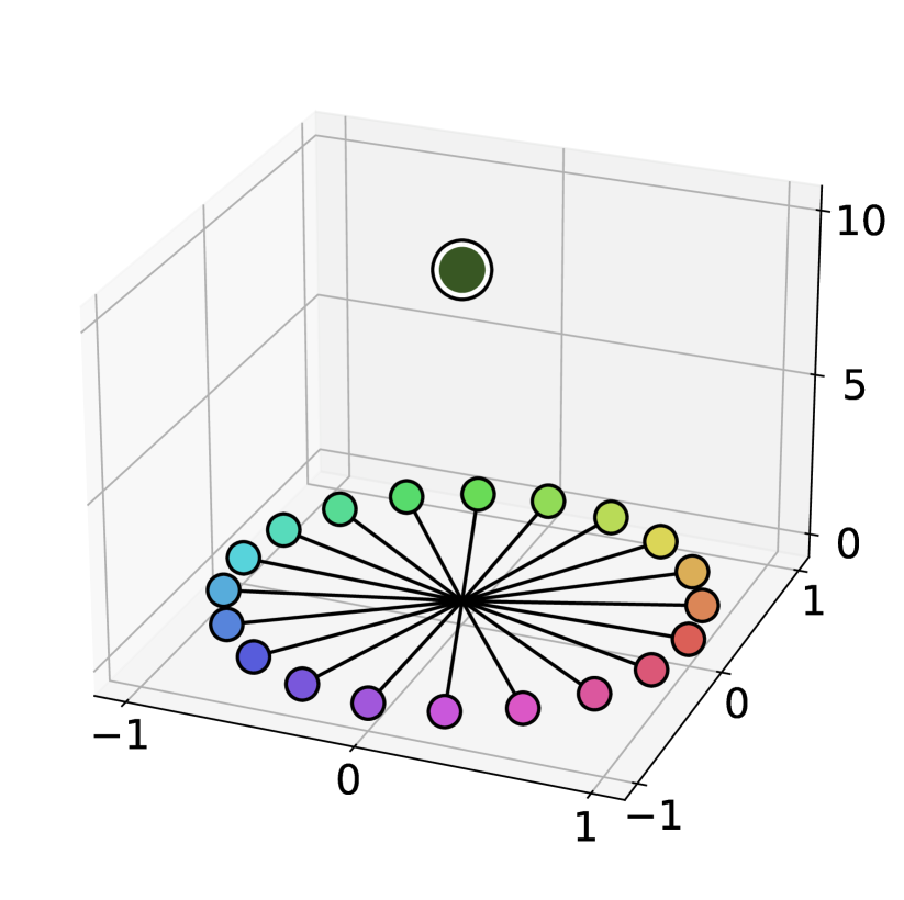
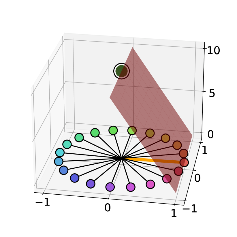
To show this theorem, we prove a property of our convex sets (i.e., polyhedral cones; see Figure 1(a)) and apply a result from the (random) POCS literature (Nedić, 2010). The proofs for this section are given in Appendix D.4.

Lemma 4.16 (Limit guarantees of random orderings).

Under a random ordering (and assumption 2.1), the iterates converge almost surely to ${\mathcal{W}^{\star}}$, such that

limkd(𝐰k,𝒲)=0,𝐰𝐰2𝐰.formulae-sequencesubscript𝑘𝑑subscript𝐰𝑘superscript𝒲0normsuperscript𝐰normsubscript𝐰2normsuperscript𝐰\lim_{k\to\infty}{d}(\mathbf{w}_{k},\mathcal{W}^{\star})=0,~{}~{}~{}\left\|{\mathbf{w}^{\star}}\right\|\leq\left\|{\mathbf{w}_{\infty}}\right\|\leq 2\left\|{\mathbf{w}^{\star}}\right\|\,.
Remark 4.17 (Beyond uniform distributions).

The result from Nedić (2010) that we used to prove Theorem 4.15, is applicable to any i.i.d. distribution with a nonzero $p_{\min}\triangleq\min_{m\in\left[{T}\right]}\Pr\left({\tau\left({{\cdot}}\right)\!=\!m}\right)>0$. In such cases, the rate from Theorem 4.15 changes to $\exp\!\left({\!-\tfrac{p_{\min}k}{4\|{\mathbf{w}^{\star}}\|^{2}R^{2}}\!}\right)$.

4.4.3 Average Iterate Analysis

So far, we analyzed the convergence of the last iterate $\mathbf{w}_{k}$. Next, we analyze the average iterate $\displaystyle{\overline{\mathbf{w}}}_{k}\triangleq\frac{1}{k}{\sum}_{t=1}^{k}\mathbf{w}_{t}$. Such analysis often allows for stronger bounds (e.g., in SGD (Shamir & Zhang, 2013), Kaczmarz methods (Morshed et al., 2022), and continual regression (Evron et al., 2022)).

Proposition 4.18 (Universal rates for the average iterate).

After $n$ cycles under a cyclic ordering ($k=nT$) we have

maxm[T]Fm(𝐰¯k)Maximum forgettingmaxm[T]d2(𝐰¯k,𝒲m)Max. dist. to any feasible setR2T2k𝐰2R2subscriptsubscript𝑚delimited-[]𝑇subscript𝐹𝑚subscript¯𝐰𝑘Maximum forgettingsubscriptsubscript𝑚delimited-[]𝑇superscript𝑑2subscript¯𝐰𝑘subscript𝒲𝑚Max. dist. to any feasible setsuperscript𝑅2superscript𝑇2𝑘superscriptnormsuperscript𝐰2superscript𝑅2\underbrace{\max_{m\in\left[{T}\right]}F_{m}({\overline{\mathbf{w}}}_{k})}_{\begin{subarray}{c}\text{Maximum forgetting}\end{subarray}}\leq\underbrace{\max_{m\in\left[{T}\right]}{d}^{2\!}\left({{\overline{\mathbf{w}}}_{k},\mathcal{W}_{m}}\right)}_{\begin{subarray}{c}\text{Max.~{}dist.~{}to any feasible set}\end{subarray}}\!R^{2}\leq\frac{T^{2}}{k}\!\left\|{\mathbf{w}^{\star}}\right\|^{2}\!R^{2}

and after k𝑘k iterations under a random ordering we have

$\displaystyle\mathop{\mathbb{E}}_{\tau}\!\Big{[}\!\underbrace{{\tfrac{1}{T}}\!\!\sum_{m=1}^{T}\!\!F_{m}({\overline{\mathbf{w}}}_{k})}_{\begin{subarray}{c}\text{Average forgetting}\end{subarray}}\!\Big{]}\!\leq\mathop{\mathbb{E}}_{\tau}\!\Big{[}\!\!\!\underbrace{{\tfrac{1}{T}}\!\!\sum_{m=1}^{T}\!\!{d}^{2\!}\left({{\overline{\mathbf{w}}}_{k},\mathcal{W}_{m}}\right)}_{\begin{subarray}{c}\text{Avg.~{}distance~{}to feasible sets}\end{subarray}}\!\!\!\Big{]}R^{2}\leq\tfrac{\left\|{\mathbf{w}^{\star}}\right\|^{2}\!R^{2}}{k}$

(implying a Tk𝐰2R2𝑇𝑘superscriptnormsuperscript𝐰2superscript𝑅2\frac{T}{k}\left\|{\mathbf{w}^{\star}}\right\|^{2}\!R^{2} bound on the expected maximum forgetting and maximum distance to any feasible set).

The proof is given in Appendix D.5.

Refer to caption

(a) Two iterations of the double exponential scheduler with two values $p=\nicefrac{{1}}{{2}},2$. $p>1$ shrinks $\mathbf{w}_{1}$ before projecting it onto $\mathcal{W}_{2}$, while $p<1$ inflates it.
Refer to caption
(b) $p>1\Longrightarrow$ Might not converge to $\mathcal{W}^{\star}$. Here, ${p\!=\!2}$, ${\lambda_{1}\!=\!\lambda\!=\!{10}^{-32}}$, ${\lambda_{6}\!\!=\!{10}^{-1024}}$. Black lines indicate changes in the directions of the weakly-regularized solutions (their actual scale is much larger).
Refer to caption
(c) $p\!>\!1\Longrightarrow$ Possibly $\left\|{\mathbf{w}_{t}}\right\|>2\left\|{\mathbf{w}^{\star}}\right\|$ (the guarantee from Thm. 4.7 does not hold). Here, $p=0.55$, ${\lambda_{1}=\lambda={10}^{-4096}}$ and the rest $\lambda_{2},\lambda_{3},\lambda_{4},\lambda_{5}$ are ${10}^{-2253},{10}^{-1239},{10}^{-681},{10}^{-375}$.
Figure 4: Illustrations and experiments for the double exponential regularization scheduling (Eq. (3) in Section 5.1).

5 Extensions

5.1 Regularization Strength Scheduling

Up to this point, we assumed that the regularization strengths in Scheme 1 are constant, i.e., $\lambda_{1}=.\hskip 0.8pt\!.\hskip 0.8pt\!.=\lambda_{k}\triangleq\lambda$. Alternatively, these strengths can vary, as done in practice in stationary settings (Lewkowycz & Gur-Ari, 2020). Related work in continual learning (Mirzadeh et al., 2020) used a learning-rate decay scheme, which can be seen as a form of varying regularization. We now aim to understand the bias and implications of varying regularization strengths.

Given $\lambda>0$, we parameterize the regularization strengths as $\lambda_{t}\!\triangleq\!\lambda_{t}(\lambda)\!>\!0$ for arbitrary functions $\lambda_{t}\!:\mathbb{R}_{>0}\!\to\!\mathbb{R}_{>0}$ holding that $\lim_{\lambda\to 0}\lambda_{t}(\lambda)\!=\!0$ and $\lim_{\lambda\to 0}\tfrac{\ln\lambda_{t-1}}{\ln\lambda_{t}}\!<\!\infty$ is well-defined $\forall t\!\in\!\left[{k}\right]$. We show that the weakly-regularized Scheme 1 (with $\lambda_{1},.\hskip 0.8pt\!.\hskip 0.8pt\!.,\lambda_{k}$) converges to the scheme below.

Scheme 3 Scheduled Sequential Max-Margin
  Initialization: $\mathbf{w}_{0}=\mathbf{0}_{D}$
  Iterative update $\forall t\!\in\![k]$: $\displaystyle\mathbf{w}_{t}\!=\!{\mathbf{P}}_{t}{\Big{(}{\big{(}{\lim_{\lambda\to 0}\!\tfrac{\ln\lambda_{t-1}}{\ln\lambda_{t}}}\big{)}\mathbf{w}_{t-1}}\Big{)}}$

Theorem 5.1 (Weakly-regularized models with scheduling).

For almost all separable datasets, when scheduling the regularization strength as described above, it holds that

$$\lim_{\lambda\to 0}\frac{\mathbf{w}_{t}^{(\lambda)}}{\|{\mathbf{w}_{t}^{(\lambda)}}\|}=\frac{\mathbf{w}_{t}}{\|{\mathbf{w}_{t}}\|},~{}~{}~{}{\forall t\!\in\!\left[{k}\right]}\,.$$

The proofs for this section are given in Appendix E & E.1.

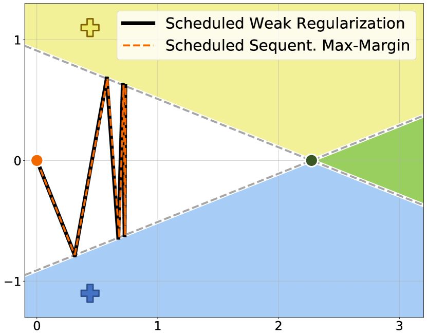
Specifically, using a double exponential scheduling rule,

$\displaystyle\lambda_{t}=\lambda_{t-1}^{p}\,({=\lambda_{1}^{p^{t-1}}\!=\lambda^{p^{t-1}}})\,,\,\,\text{ for some $p>0$ ,}$ (3)

the update rule in Scheme 3 becomes ${\mathbf{w}_{t}\!=\!{\mathbf{P}}_{t}\big{(}{\tfrac{1}{p}\mathbf{w}_{t-1}}\big{)}}$. We illustrate this in Figure 4(a).

In this case, in contrast to the $p\!=\!1$ case, even when tasks recur we may not converge near the min-norm solution or the feasibility set, as demonstrated in the next examples.

Example 2 ($p>1\Longrightarrow$ Possibly $\mathbf{w}_{\infty}\notin\mathcal{W}^{\star}$).

In Figure 4(b), we cycle between two tasks using Schemes 1 and 3 with $p=2$. The strengths decay like $\lambda,\lambda^{2},\lambda^{4},\lambda^{8}$, and so on. Note that both schemes agree. Unlike the constant $\lambda$ case (Thm. 4.12), we do not converge to the offline set $\mathcal{W}^{\star}$.

More generally, we prove that when $p>1$, the limit distance from the offline feasible set $\mathcal{W}^{\star}$ can be arbitrarily bad.

Proposition 5.2.

There exists a construction of two jointly-separable tasks with $R=1$, in which the iterates of the cyclic ordering do not converge to $\mathcal{W}^{\star}$, for any $p>1$. Specifically, for any ${p>1,\left\|{\mathbf{w}^{\star}}\right\|>1}$, it holds that

$\displaystyle\lim_{k\to\infty}\frac{{d}(\mathbf{w}_{k},\mathcal{W}^{\star})}{\|{\mathbf{w}^{\star}}\|}=\frac{\left\|{\mathbf{w}^{\star}}\right\|^{2}(p-1)}{2+\left\|{\mathbf{w}^{\star}}\right\|^{2}(p-1)}\sqrt{1-\tfrac{1}{\left\|{\mathbf{w}^{\star}}\right\|^{2}}}\,.$
Example 3 ($p<1\Longrightarrow$ No optimality guarantees on $\mathbf{w}_{t}$).

In Figure 4(c), we run both Schemes 1 and 3 with $p=0.55$ for one “pass” over the tasks. The strengths increase like $\lambda,\lambda^{0.55},\lambda^{0.303},\lambda^{0.166}$, and so on (however, our analysis still requires that $\lambda\to 0$; see Remark E.1). Note that the iterates of both schemes agree. Unlike the guarantees for the constant $\lambda$ case (Theorem 4.7), here $\left\|{\mathbf{w}_{5}}\right\|>2\left\|{\mathbf{w}^{\star}}\right\|$.

Roughly speaking, adversarial placements of examples (i.e., feasible sets) can make the iterates $(\mathbf{w}_{t})$ grow like $\mathcal{O}\left({p^{-t}}\right)$, even in an almost orthogonal direction to the min-norm $\mathbf{w}^{\star}$.

Remark 5.3.

We analyzed the double exponential rule (3) since “milder” rules (e.g., $\lambda_{t}\!=\!c^{t}\lambda$ for $c\!=\!\mathcal{O}(1)$) do not influence Scheme 3, thus not affecting Scheme 1 when ${\lambda\!\to\!0}$. Even a rule like ${\lambda_{t}\!=\!\lambda^{t}}$ implies ${\lim_{\lambda\to 0}\!\tfrac{\ln\lambda_{t-1}}{\ln\lambda_{t}}\!=\!1\!-\!\frac{1}{t}}$ and becomes insignificant as $t$ increases.

5.2 Weighted Regularization

So far, we analyzed unweighted regularizers in Scheme 1. Most regularization methods for continual learning employ weighted norms (e.g., Kirkpatrick et al. (2017); Zenke et al. (2017); Aljundi et al. (2018)). Now, we focus on such norms and link them to Sequential Max-Margin when $\lambda\to 0$.

Given $\mathbf{B}_{1},.\hskip 0.8pt\!.\hskip 0.8pt\!.,\mathbf{B}_{k}\!\succ\!\mathbf{0}_{D\times D}$, we define the following scheme.

Scheme 4 Weighted Sequential Max-Margin
  Initialization: $\mathbf{w}_{0}=\mathbf{0}_{D}$
  Iterative update for each task $t\in\left[{k}\right]$:
$\displaystyle\mathbf{w}_{t}={{\mathbf{P}}_{t}}\left({\mathbf{w}_{t-1}}\right)\triangleq{\operatorname*{argmin}}_{\mathbf{w}}\,$ $\displaystyle\!\left\|{\mathbf{w}-{\mathbf{w}}_{t-1}}\right\|^{2}_{\mathbf{B}_{t}}$
s.t. $\displaystyle\,y\mathbf{w}^{\top}\mathbf{x}\!\geq\!1,\,\forall(\mathbf{x},y)\!\in\!S_{t}$
Theorem 5.4 (Weak weighted regularization).

For almost all separable datasets and bounded weighting schemes (holding ${0\!<\!\mu\!\leq\!\sigma_{\min}(\mathbf{B}_{t})\!\leq\!\sigma_{\max}(\mathbf{B}_{t})\!\leq\!M\!<\!\infty}$), in the limit of $\lambda\!\to\!0$, Schemes 1 and 4 coincide. That is, $\forall t\!\in\!\left[{k}\right]$, it holds that $\displaystyle\lim_{\lambda\to 0}\frac{\mathbf{w}_{t}^{(\lambda)}}{\|{\mathbf{w}_{t}^{(\lambda)}}\|}=\frac{\mathbf{w}_{t}}{\|{\mathbf{w}_{t}}\|}$.

The proofs for this section are given in Appendix E & LABEL:app:weighted.

Practically, most regularization methods use weighting matrices based on Fisher information (FI) (Benzing, 2022). We present a novel result showing that in continual regression, such weighting schemes prevent forgetting (thus forming an “ideal continual learner” as defined by Peng et al. (2023)).

Proposition 5.5.

Using a Fisher-information-based weighting scheme of $\mathbf{B}_{t}=\sum_{i=1}^{t-1}\sum_{\mathbf{x}\in S_{i}}\mathbf{x}\mathbf{x}^{\top}$, there is no forgetting in (realizable) continual linear333A similar guarantee also applies more broadly, for linear networks of any depth and non-linear networks in the NTK regime. regression.

In contrast, below we show a simple example where such weighting schemes, even when using the full FI matrices, do not prevent forgetting in continual linear classification.

Figure 5: A 2-dimensional setting with solely two orthogonal examples $\mathbf{x}_{1}\!\perp\!\mathbf{x}_{2}$ in the 1st task. Here, the iterate $\mathbf{w}_{1}$ holds ${\mathbf{w}_{1}^{\top}\mathbf{x}_{1}\!=\!\mathbf{w}_{1}^{\top}\mathbf{x}_{2}\!=\!1}$, implying a FI matrix of ${\mathbf{B}_{2}\!\propto\!\sum_{i\in\left[{2}\right]}\mathbf{x}_{i}\mathbf{x}_{i}^{\top}\!=\!\mathbf{I}}$. Then, FI weighting (dotted) reverts to vanilla L2 regularization (dashed) which does not prevent forgetting.
In contrast, the FI matrices in high dimensions are often non-invertible. Then, the learner can move freely in directions orthogonal to previous data ($\left\|{\cdot}\right\|_{\mathbf{B}_{t}}$ is no longer a “proper” norm), thus avoiding forgetting.
See further examples in App. LABEL:app:weighted_examples.
Refer to caption

An interesting question arises: Are there general weighting schemes that can prevent forgetting in Scheme 4? We find this to be an exciting direction for future research.

6 Related Work

Many papers have investigated various aspects of catastrophic forgetting, including when it occurs (Evron et al., 2022), strategies to avoid it (Peng et al., 2023), the influence of task similarity (Lee et al., 2021), its impact on transferability (Chen et al., 2023), and other related factors. A sound understanding of forgetting can potentially advance the continual learning field significantly.

Throughout our paper, we discussed many connections to other works from many fields. Interestingly, our Sequential Max-Margin (SMM) scheme can be seen as a hard variant of the Adaptive SVM algorithm (Yang et al., 2007), which was previously used to practically tackle domain adaptation and transfer learning. (e.g., in Li (2007); Pentina et al. (2015); Tang et al. (2022)). To the best of our knowledge, our paper is the first to highlight the connection between regularization methods for continual learning and Adaptive SVM.

For the special case where each task has one datapoint, the SMM scheme corresponds to the online Passive-Aggressive algorithm (Crammer et al., 2006). If additionally, we consider only two tasks learned in a cyclic ordering, the regret after training task $t$ is related (but not identical) to the forgetting (see Remark 4.2). Consequently, our forgetting bound in Prop. 4.13 matches the regret bound in their Theorem 2.

7 Discussion and Future Work

7.1 Early Stopping

When training a single task, it is well known that explicit regularization is related to early stopping. In linear classification with an exponential loss, Rosset et al. (2004) showed that the regularization path converges (in the $\lambda\rightarrow 0$ limit) to the hard-margin SVM, which is also the limit of the optimization path (Soudry et al., 2018). In regression, Ali et al. (2019) connected early stopping to ridge regression.

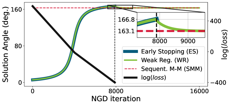
Contrastingly, when learning a sequence of tasks, explicit regularization and early stopping can behave differently. We first discuss a case where both methods lead to SMM. More generally, we demonstrate that solutions may differ.

Consider a task sequence with $1$ sample $(\mathbf{x}_{t},y_{t})$ per task.444Equivalently, $2$ samples $(\mathbf{x}_{t},y_{t})$ and $(-\mathbf{x}_{t},-y_{t})$. We minimize the exponential loss of each task $t$ with gradient flow (GF) until $L_{t}(\mathbf{w})\!\triangleq\!\exp(-y_{t}\mathbf{x}_{t}^{\top}\mathbf{w})\!=\!\epsilon$ for a fixed $\epsilon\!<\!1$, yielding a predictor $\mathbf{w}_{t}^{(\epsilon)}$. Denote the “normalized” predictor by ${\hat{\mathbf{w}}_{t}^{(\epsilon)}\!=\!{\mathbf{w}_{t}^{(\epsilon)}}/\ln({1}/{\epsilon})}$. Since GF stays in the data span, we have ${\mathbf{w}_{t}^{(\epsilon)}\!=\!\mathbf{w}_{t-1}^{(\epsilon)}\!+\!\alpha_{t}y_{t}\mathbf{x}_{t}}$ for some $\alpha_{t}>0$. The early stopping implies $y_{t}\mathbf{x}_{t}^{\top}{\mathbf{w}}_{t}^{(\epsilon)}\!=\!\ln({1}/{\epsilon})$, and thus $y_{t}\mathbf{x}_{t}^{\top}\hat{\mathbf{w}}_{t}^{(\epsilon)}\!=\!1$. Hence, $\hat{\mathbf{w}}_{t}^{(\epsilon)}$ holds the KKT conditions of the SMM, i.e., ${\hat{\mathbf{w}}_{t}^{(\epsilon)}\!=\!\operatorname*{argmin}_{\mathbf{w}}\!\big{\|}{\mathbf{w}\!-\!\hat{\mathbf{w}}_{t-1}^{(\epsilon)}}\big{\|}^{2}\,\textrm{s.t.}\,\,y_{t}\mathbf{x}_{t}^{\top}\mathbf{w}\geq 1}$ (where ${\hat{\alpha}_{t}\triangleq\left({\alpha_{t}\,/\ln({1}/{\epsilon})}\right)>0}$ is the dual variable).555 If iteration $t$ begins and we already have $L_{t}({\mathbf{w}}_{t-1}^{(\epsilon)})\!<\!\epsilon$ and $y_{t}\mathbf{x}_{t}^{\top}\hat{\mathbf{w}}_{t-1}^{(\epsilon)}\!\geq\!1$, both ES and SMM will not change their solutions. In the general case (i.e., more than one sample per task), early stopping might not agree with SMM, as depicted below.

Refer to caption
Figure 6: Comparing the weakly-regularized (WR) and early stopping (ES) schemes. We train $2$ tasks: $S_{1}=\{(10,1)\}$, $S_{2}\!=\!\{(-10,1),(-15,0.5)\}$ (where all points are labeled $+1$). We plot the angle of different predictors ($\angle(\mathbf{w},\left[\begin{subarray}{c}1\\ 0\end{subarray}]\right])$) while training on the 2nd task. For instance, the Sequential Max-Margin (SMM) solution for that task is $163.1^{\circ}$. For ES, we train both tasks with normalized GD (NGD) until their loss is ${\epsilon=e^{-200}}$. Importantly, ES stops when the loss of the 2nd task, shown in the secondary y-axis, is $e^{-200}$ and the angle is $166.8^{\circ}$. For WR, we set ${\lambda\!=\!e^{-200}}$ and solve Eq. (1) by running NGD to convergence. For the 2nd task, we initialize the NGD by $\mathbf{w}_{1}^{(\lambda)}$. Unlike ES, the WR solution does converge to $163.1^{\circ}$ like SMM, as guaranteed by Theorem 3.1. Further details in App. F.

7.2 Future Work

There are several interesting avenues for future work, e.g., extending our results to non-separable data (perhaps in the spirit of Yang et al. (2007)), multiclass classification with cross-entropy loss (similarly to Appendix 4.1 in Soudry et al. (2018)), or non-linear models. One can also try to derive forgetting bounds for weighted regularization schemes and look for optimal weighting matrices. Another challenging but rewarding avenue is to extend our analysis to finite regularization strengths $(\lambda_{t})$. Finally, it is interesting to understand the exact algorithmic bias for early stopping in continual learning and its relation to explicit regularization.

Acknowledgements

We thank Lior Alon (MIT) for the fruitful discussions. The research of DS was Funded by the European Union (ERC, A-B-C-Deep, 101039436). Views and opinions expressed are however those of the author only and do not necessarily reflect those of the European Union or the European Research Council Executive Agency (ERCEA). Neither the European Union nor the granting authority can be held responsible for them. DS also acknowledges the support of Schmidt Career Advancement Chair in AI. NS was partially supported by the Simons Foundation and NSF-IIS/CCF awards.

References

  • Agmon (1954) Agmon, S. The relaxation method for linear inequalities. Canadian Journal of Mathematics, 6:382–392, 1954.
  • Ali et al. (2019) Ali, A., Kolter, J. Z., and Tibshirani, R. J. A continuous-time view of early stopping for least squares regression. In AISTATS, volume 89 of Proceedings of Machine Learning Research, pp.  1370–1378. PMLR, 2019.
  • Aljundi et al. (2018) Aljundi, R., Babiloni, F., Elhoseiny, M., Rohrbach, M., and Tuytelaars, T. Memory aware synapses: Learning what (not) to forget. In Proceedings of the European Conference on Computer Vision (ECCV), pp.  139–154, 2018.
  • Asanuma et al. (2021) Asanuma, H., Takagi, S., Nagano, Y., Yoshida, Y., Igarashi, Y., and Okada, M. Statistical mechanical analysis of catastrophic forgetting in continual learning with teacher and student networks. Journal of the Physical Society of Japan, 90(10):104001, Oct 2021.
  • Bauschke (2001) Bauschke, H. H. Projection algorithms: results and open problems. In Studies in Computational Mathematics, volume 8, pp. 11–22. Elsevier, 2001.
  • Bauschke & Borwein (1993) Bauschke, H. H. and Borwein, J. M. On the convergence of von neumann’s alternating projection algorithm for two sets. Set-Valued Analysis, 1(2):185–212, 1993.
  • Bauschke et al. (2011) Bauschke, H. H., Combettes, P. L., et al. Convex analysis and monotone operator theory in Hilbert spaces, volume 408. Springer, 2011.
  • Belkin et al. (2018) Belkin, M., Ma, S., and Mandal, S. To understand deep learning we need to understand kernel learning. In International Conference on Machine Learning, pp. 541–549. PMLR, 2018.
  • Bennani et al. (2020) Bennani, M. A., Doan, T., and Sugiyama, M. Generalisation guarantees for continual learning with orthogonal gradient descent. arXiv preprint arXiv:2006.11942, 2020.
  • Benzing (2022) Benzing, F. Unifying regularisation methods for continual learning. In International Conference on Artificial Intelligence and Statistics. PMLR, 2022.
  • Borwein et al. (2014) Borwein, J. M., Li, G., and Yao, L. Analysis of the convergence rate for the cyclic projection algorithm applied to basic semialgebraic convex sets. SIAM Journal on Optimization, 24(1):498–527, 2014.
  • Boyd & Vandenberghe (2004) Boyd, S. and Vandenberghe, L. Convex optimization. Cambridge university press, 2004.
  • Chen et al. (2023) Chen, J., Nguyen, T., Gorur, D., and Chaudhry, A. Is forgetting less a good inductive bias for forward transfer? In The Eleventh International Conference on Learning Representations, 2023.
  • Cossu et al. (2022) Cossu, A., Graffieti, G., Pellegrini, L., Maltoni, D., Bacciu, D., Carta, A., and Lomonaco, V. Is class-incremental enough for continual learning? Frontiers in Artificial Intelligence, 5, 2022.
  • Crammer et al. (2006) Crammer, K., Dekel, O., Keshet, J., Shalev-Shwartz, S., and Singer, Y. Online passive-aggressive algorithms. Journal of Machine Learning Research, 7(19):551–585, 2006.
  • Deutsch & Hundal (2006a) Deutsch, F. and Hundal, H. The rate of convergence for the cyclic projections algorithm i: Angles between convex sets. Journal of Approximation Theory, 142(1):36–55, 2006a.
  • Deutsch & Hundal (2006b) Deutsch, F. and Hundal, H. The rate of convergence for the cyclic projections algorithm ii: norms of nonlinear operators. Journal of Approximation Theory, 142(1):56–82, 2006b.
  • Deutsch & Hundal (2008) Deutsch, F. and Hundal, H. The rate of convergence for the cyclic projections algorithm iii: Regularity of convex sets. Journal of Approximation Theory, 155(2):155–184, 2008.
  • Doan et al. (2021) Doan, T., Abbana Bennani, M., Mazoure, B., Rabusseau, G., and Alquier, P. A theoretical analysis of catastrophic forgetting through the ntk overlap matrix. In Proceedings of The 24th International Conference on Artificial Intelligence and Statistics, pp.  1072–1080, 2021.
  • Du et al. (2019) Du, S., Lee, J., Li, H., Wang, L., and Zhai, X. Gradient descent finds global minima of deep neural networks. In International conference on machine learning, pp. 1675–1685. PMLR, 2019.
  • Evron et al. (2022) Evron, I., Moroshko, E., Ward, R., Srebro, N., and Soudry, D. How catastrophic can catastrophic forgetting be in linear regression? In Conference on Learning Theory (COLT), pp.  4028–4079. PMLR, 2022.
  • Goldfarb & Hand (2023) Goldfarb, D. and Hand, P. Analysis of catastrophic forgetting for random orthogonal transformation tasks in the overparameterized regime. In International Conference on Artificial Intelligence and Statistics, pp.  2975–2993. PMLR, 2023.
  • Goodfellow et al. (2013) Goodfellow, I. J., Mirza, M., Xiao, D., Courville, A., and Bengio, Y. An empirical investigation of catastrophic forgetting in gradient-based neural networks. arXiv preprint arXiv:1312.6211, 2013.
  • Gubin et al. (1967) Gubin, L., Polyak, B. T., and Raik, E. The method of projections for finding the common point of convex sets. USSR Computational Mathematics and Mathematical Physics, 7(6):1–24, 1967.
  • Halperin (1962) Halperin, I. The product of projection operators. Acta Sci. Math.(Szeged), 23(1):96–99, 1962.
  • Hoi et al. (2021) Hoi, S. C., Sahoo, D., Lu, J., and Zhao, P. Online learning: A comprehensive survey. Neurocomputing, 459:249–289, 2021. ISSN 0925-2312.
  • Ji & Telgarsky (2020) Ji, Z. and Telgarsky, M. Polylogarithmic width suffices for gradient descent to achieve arbitrarily small test error with shallow relu networks. In International Conference on Learning Representations, 2020.
  • Kirkpatrick et al. (2017) Kirkpatrick, J., Pascanu, R., Rabinowitz, N., Veness, J., Desjardins, G., Rusu, A. A., Milan, K., Quan, J., Ramalho, T., Grabska-Barwinska, A., et al. Overcoming catastrophic forgetting in neural networks. Proceedings of the national academy of sciences, 114(13):3521–3526, 2017.
  • Lee et al. (2021) Lee, S., Goldt, S., and Saxe, A. Continual learning in the teacher-student setup: Impact of task similarity. In International Conference on Machine Learning, pp. 6109–6119. PMLR, 2021.
  • Lesort et al. (2022) Lesort, T., Ostapenko, O., Misra, D., Arefin, M. R., Rodríguez, P., Charlin, L., and Rish, I. Scaling the number of tasks in continual learning. arXiv preprint arXiv:2207.04543, 2022.
  • Lewkowycz & Gur-Ari (2020) Lewkowycz, A. and Gur-Ari, G. On the training dynamics of deep networks with $l\_2$ regularization. Advances in Neural Information Processing Systems, 33:4790–4799, 2020.
  • Li et al. (2023) Li, H., Wu, J., and Braverman, V. Fixed design analysis of regularization-based continual learning. arXiv preprint arXiv:2303.10263, 2023.
  • Li (2007) Li, X. Regularized adaptation: Theory, algorithms and applications. Citeseer, 2007.
  • Lubana et al. (2022) Lubana, E. S., Trivedi, P., Koutra, D., and Dick, R. How do quadratic regularizers prevent catastrophic forgetting: The role of interpolation. In Conference on Lifelong Learning Agents, pp.  819–837. PMLR, 2022.
  • McCloskey & Cohen (1989) McCloskey, M. and Cohen, N. J. Catastrophic interference in connectionist networks: The sequential learning problem. In Psychology of learning and motivation, volume 24, pp. 109–165. Elsevier, 1989.
  • Mirzadeh et al. (2020) Mirzadeh, S. I., Farajtabar, M., Pascanu, R., and Ghasemzadeh, H. Understanding the role of training regimes in continual learning. In Larochelle, H., Ranzato, M., Hadsell, R., Balcan, M. F., and Lin, H. (eds.), Advances in Neural Information Processing Systems, volume 33, pp.  7308–7320. Curran Associates, Inc., 2020.
  • Morshed et al. (2022) Morshed, M. S., Islam, M. S., and Noor-E-Alam, M. Sampling kaczmarz-motzkin method for linear feasibility problems: generalization and acceleration. Mathematical Programming, 194(1-2):719–779, 2022.
  • Nedić (2010) Nedić, A. Random projection algorithms for convex set intersection problems. In 49th IEEE Conference on Decision and Control (CDC), pp. 7655–7660. IEEE, 2010.
  • Needell & Tropp (2014) Needell, D. and Tropp, J. A. Paved with good intentions: analysis of a randomized block kaczmarz method. Linear Algebra and its Applications, 441:199–221, 2014.
  • Novikoff (1962) Novikoff, A. B. On convergence proofs on perceptrons. In Proceedings of the Symposium on the Mathematical Theory of Automata, volume 12, pp.  615–622, New York, NY, USA, 1962. Polytechnic Institute of Brooklyn.
  • Peng et al. (2023) Peng, L., Giampouras, P., and Vidal, R. The ideal continual learner: An agent that never forgets. In International Conference on Machine Learning, 2023.
  • Pentina et al. (2015) Pentina, A., Sharmanska, V., and Lampert, C. H. Curriculum learning of multiple tasks. In Proceedings of the IEEE Conference on Computer Vision and Pattern Recognition, pp.  5492–5500, 2015.
  • Reich & Zalas (2023) Reich, S. and Zalas, R. Polynomial estimates for the method of cyclic projections in hilbert spaces. Numerical Algorithms, pp.  1–26, 2023.
  • Robins (1995) Robins, A. Catastrophic forgetting, rehearsal and pseudorehearsal. Connection Science, 7(2):123–146, 1995.
  • Rolnick et al. (2019) Rolnick, D., Ahuja, A., Schwarz, J., Lillicrap, T., and Wayne, G. Experience replay for continual learning. Advances in Neural Information Processing Systems, 32, 2019.
  • Rosset et al. (2004) Rosset, S., Zhu, J., and Hastie, T. J. Margin maximizing loss functions. In Advances in neural information processing systems, pp. 1237–1244, 2004.
  • Shalev-Shwartz et al. (2012) Shalev-Shwartz, S. et al. Online learning and online convex optimization. Foundations and Trends® in Machine Learning, 4(2):107–194, 2012.
  • Shamir & Zhang (2013) Shamir, O. and Zhang, T. Stochastic gradient descent for non-smooth optimization: Convergence results and optimal averaging schemes. In International conference on machine learning, pp.  71–79. PMLR, 2013.
  • Sidford (2020) Sidford, A. Ms&e 213/cs 269o: Chapter 3-convexity, 2020.
  • Smith et al. (2023) Smith, J. S., Tian, J., Hsu, Y.-C., and Kira, Z. A closer look at rehearsal-free continual learning. In CVPR Workshop on Continual Learning in Computer Vision, 2023.
  • Soudry et al. (2018) Soudry, D., Hoffer, E., Shpigel Nacson, M., Gunasekar, S., and Srebro, N. The implicit bias of gradient descent on separable data. JMLR, 2018.
  • Stojanov et al. (2019) Stojanov, S., Mishra, S., Thai, N. A., Dhanda, N., Humayun, A., Yu, C., Smith, L. B., and Rehg, J. M. Incremental object learning from contiguous views. In Proceedings of the IEEE/CVF Conference on Computer Vision and Pattern Recognition, pp.  8777–8786, 2019.
  • Tang et al. (2022) Tang, J., Lin, K.-Y., and Li, L. Using domain adaptation for incremental svm classification of drift data. Mathematics, 10(19):3579, 2022.
  • Von Neumann (1949) Von Neumann, J. On rings of operators. reduction theory. Annals of Mathematics, pp.  401–485, 1949.
  • Wei et al. (2019) Wei, C., Lee, J. D., Liu, Q., and Ma, T. Regularization matters: Generalization and optimization of neural nets vs their induced kernel. Advances in Neural Information Processing Systems, 32, 2019.
  • Woodworth et al. (2020) Woodworth, B., Gunasekar, S., Lee, J. D., Moroshko, E., Savarese, P., Golan, I., Soudry, D., and Srebro, N. Kernel and rich regimes in overparametrized models. In Conference on Learning Theory, pp.  3635–3673. PMLR, 2020.
  • Yang et al. (2007) Yang, J., Yan, R., and Hauptmann, A. G. Adapting svm classifiers to data with shifted distributions. In Seventh IEEE international conference on data mining workshops (ICDMW 2007), pp.  69–76. IEEE, 2007.
  • Yoon et al. (2018) Yoon, J., Yang, E., Lee, J., and Hwang, S. J. Lifelong learning with dynamically expandable networks. In International Conference on Learning Representations, 2018.
  • Zenke et al. (2017) Zenke, F., Poole, B., and Ganguli, S. Continual learning through synaptic intelligence. In International Conference on Machine Learning, pp. 3987–3995. PMLR, 2017.

Appendix A Comparison: Continual Linear Classification vs. Continual Linear Regression

Continual Linear Classification (Ours) Continual Linear Regression (Evron et al., 2022)
Fundamental mapping (proven algorithmic bias)
Continual linear classification with
weakly-regularized exponential losses
converges to
a Sequential Max-Margin scheme
(Theorem 3.1)
Continual linear regression
with unregularized losses,
solved sequentially with vanilla (S)GD,
implicitly performs successive projections
(their Eq. (5))
Feasible sets
Closed, convex, and affine
polyhedral cones
(Assumption 2.1)
Closed affine subspaces
(their Eq. (4))
Projection operators
Projection onto Convex Sets (POCS);
Challenging to analyze
(Eq. (2))
Affine projections;
Easy to analyze
(their Eq. (5))
Optimality guarantees
$\left\|{\mathbf{w}_{t}}\right\|\leq 2\left\|{\mathbf{w}^{\star}}\right\|$
(Lemma 4.7)
$\left\|{\mathbf{w}_{t}}\right\|\leq\left\|{\mathbf{w}^{\star}}\right\|$
$\mathbf{w}_{t}\in\mathcal{W}^{\star}\Longrightarrow\mathbf{w}_{t}=\mathbf{w}^{\star}$
Adversarial construction
Arbitrarily bad quantities
$\displaystyle 1=\frac{1}{\left\|{\mathbf{w}^{\star}}\right\|^{2}R^{2}}\lim_{T\to\infty}\max_{m\in\left[{T}\right]}F_{m}(\mathbf{w}_{t})\leq\frac{1}{\left\|{\mathbf{w}^{\star}}\right\|^{2}}\lim_{T\to\infty}{d}^{2}\left({\mathbf{w}_{t},\mathcal{W}^{\star}}\right)\leq 1$
(our Section 4.2, their Section 4.2)
Fisher-based regularization
Does not prevent forgetting
(Figure 5, Appendix LABEL:app:weighted_examples)
Prevents forgetting
(our Prop. 5.5)
Linear regularity
Holds
$\displaystyle{d}^{2}\!\left({\mathbf{w}_{t},\mathcal{W}^{\star}}\right)\leq 4\!\left\|{\mathbf{w}}\right\|^{2}\!R^{2}\!\max_{m\in\left[{T}\right]}\!{d}^{2}\!\left({\mathbf{w}_{t},\mathcal{W}_{m}}\right)$
(Lemma 4.8)
Does not hold
Nontrivial bounds on distance to the feasible set ${d}^{2}\left({\mathbf{w}_{t},\mathcal{W}^{\star}}\right)$ depending on the problem complexity $\left\|{\mathbf{w}^{\star}}\right\|^{2}\!R^{2}$ Nontrivial bounds on forgetting depending on the problem complexity $\left\|{\mathbf{w}^{\star}}\right\|^{2}\!R^{2}$
Possible due to regularity;
Exponential decrease (linear convergence)
(Table 1, Theorems 4.12 and 4.15)
Impossible
(e.g., their Section 5.1)
Possible universal bounds
(see below)
Universal bounds on forgetting under cyclic orderings (independent of $\left\|{\mathbf{w}^{\star}}\right\|^{2}\!R^{2}$)
$\displaystyle{\frac{2T^{2}}{\sqrt{k}}}$
(Proposition 4.13)
$\displaystyle\min\left({\frac{T^{2}}{\sqrt{k}},\frac{T^{2}D}{2k}}\right)$
(their Theorem 11)
Universal bounds on forgetting under random orderings (independent of $\left\|{\mathbf{w}^{\star}}\right\|^{2}\!R^{2}$) Unclear if possible
$\displaystyle\frac{9D}{k}$
(their Theorem 13)

Appendix B Proofs for Algorithmic Bias in Regularization Methods (Section 3)

Remark B.1 (Simplification).

For ease of notation, throughout our appendices, we redefine the samples so as to subsume their labels. That is, we handle only positive labels by redefining each $y\mathbf{x}\longmapsto\mathbf{x}$. This notation is common in theoretical papers (e.g., Soudry et al. (2018)).

B.1 Auxiliary Lemmas

We first present two auxiliary results that we need for our main proof.

Lemma B.2.

Let $f:\mathbb{R}^{D}\to\mathbb{R}$ be a $\mu$-strongly convex objective function (holding $\nabla^{2}f(\mathbf{w})\succeq\mu\mathbf{I}$ for some $\mu>0$). Then, for any $\mathbf{w}\in\mathbb{R}^{D}$, the (Euclidean) distance between $\mathbf{w}$ and $\mathbf{w}^{\star}$ (the minimizer of the objective $f$), can be upper bounded by:

$$\left\|{\mathbf{w}-\mathbf{w}^{\star}}\right\|\leq\frac{1}{\mu}\left\|{\nabla f(\mathbf{w})}\right\|\,.$$
Proof.

This lemma is a known convex optimization result (e.g., see Lemma 10 in Sidford (2020)). We prove it here for the sake of completeness.

We make use of the following property of strongly convex functions.

Property (9.8) from Boyd & Vandenberghe (2004).

Let $f:\mathbb{R}^{D}\to\mathbb{R}$ be a $\mu$-strongly convex objective function (holding $\nabla^{2}f(\mathbf{w})\succeq\mu\mathbf{I}$ for some $\mu>0$). Then, for any $\mathbf{x},\mathbf{y}\in\mathbb{R}^{D}$, we have

$$f(\mathbf{y})\geq f(\mathbf{x})+\nabla f(\mathbf{x})^{\top}\left({\mathbf{y}-\mathbf{x}}\right)+\frac{\mu}{2}\left\|{\mathbf{y}-\mathbf{x}}\right\|^{2}\,.$$

Using the above property, we prove our lemma, which is a slightly stronger result than Property (9.11) in Boyd & Vandenberghe (2004). Our proof follows the one by Sidford (2020), and is brought here for completeness.

First, we set $\mathbf{x}=\mathbf{w}^{\star},\mathbf{y}=\mathbf{w}$ (from our lemma). Since $\mathbf{w}^{\star}$ is a (global) minimizer, its gradient is zero, i.e., $\nabla f(\mathbf{w}^{\star})\!=\!\mathbf{0}_{D}$. We thus get that

$\displaystyle f(\mathbf{w})$ $\displaystyle\geq f(\mathbf{w}^{\star})+\underbrace{\nabla f(\mathbf{w}^{\star})^{\top}}_{=\mathbf{0}_{D}}\left({\mathbf{w}-\mathbf{w}^{\star}}\right)+\frac{\mu}{2}\left\|{\mathbf{w}-\mathbf{w}^{\star}}\right\|^{2}$
$\displaystyle f(\mathbf{w})-f(\mathbf{w}^{\star})$ $\displaystyle\geq\frac{\mu}{2}\left\|{\mathbf{w}-\mathbf{w}^{\star}}\right\|^{2}\,.$

Using the optimality of $\mathbf{w}^{\star}$, we get that

$\displaystyle\forall\mathbf{w}\in\mathbb{R}^{D}:~{}f(\mathbf{w}^{\star})=\min_{\mathbf{y}}f(\mathbf{y})$ $\displaystyle\geq\min_{\mathbf{y}}\left({f(\mathbf{w})+\nabla f(\mathbf{w})^{\top}\left({\mathbf{y}-\mathbf{w}}\right)+\frac{\mu}{2}\left\|{\mathbf{y}-\mathbf{w}}\right\|^{2}}\right)$
$\displaystyle=f(\mathbf{w})+\min_{\mathbf{y}}\left({\nabla f(\mathbf{w})^{\top}\left({\mathbf{y}-\mathbf{w}}\right)+\frac{\mu}{2}\left\|{\mathbf{y}-\mathbf{w}}\right\|^{2}}\right)\,.$

Then, by plugging in the minimizer of the right term, we get

$\displaystyle\forall\mathbf{w}\in\mathbb{R}^{D}:~{}f(\mathbf{w}^{\star})$ $\displaystyle\geq f(\mathbf{w})+\nabla f(\mathbf{w})^{\top}\Big{(}{\mathbf{w}-\frac{1}{\mu}\nabla f(\mathbf{w})-\mathbf{w}}\Big{)}+\frac{\mu}{2}\Big{\|}{\mathbf{w}-\frac{1}{\mu}\nabla f(\mathbf{w})-\mathbf{w}}\Big{\|}^{2}$
$\displaystyle=f(\mathbf{w})-\frac{1}{\mu}\nabla f(\mathbf{w})^{\top}\nabla f(\mathbf{w})+\frac{\mu}{2}\Big{\|}{\frac{1}{\mu}\nabla f(\mathbf{w})}\Big{\|}^{2}=f(\mathbf{w})-\frac{1}{\mu}\big{\|}{\nabla f(\mathbf{w})}\big{\|}^{2}+\frac{1}{2\mu}\big{\|}{\nabla f(\mathbf{w})}\big{\|}^{2}$
$\displaystyle=f(\mathbf{w})-\frac{1}{2\mu}\big{\|}{\nabla f(\mathbf{w})}\big{\|}^{2}$
$\displaystyle\frac{1}{2\mu}\big{\|}{\nabla f(\mathbf{w})}\big{\|}^{2}$ $\displaystyle\geq f(\mathbf{w})-f(\mathbf{w}^{\star})\,.$

Overall, we showed that $\forall\mathbf{w}\in\mathbb{R}^{D}$, it holds that

$\displaystyle\frac{1}{2\mu}\big{\|}{\nabla f(\mathbf{w})}\big{\|}^{2}\geq f(\mathbf{w})-f(\mathbf{w}^{\star})\geq\frac{\mu}{2}\left\|{\mathbf{w}-\mathbf{w}^{\star}}\right\|^{2}~{}~{}~{}\Longrightarrow~{}~{}~{}\frac{1}{\mu^{2}}\big{\|}{\nabla f(\mathbf{w})}\big{\|}^{2}\geq\left\|{\mathbf{w}-\mathbf{w}^{\star}}\right\|^{2}\,,$

as required. ∎

Lemma B.3.

Let $c_{1},\dots,c_{k}\in\mathbb{R}_{\geq 0}$ and let $\mathbf{B}_{1},\dots,\mathbf{B}_{k}\succ\mathbf{0}_{D\times D}$. Consider sequentially solving $k$ separable tasks $(S_{t}=(\mathbf{X}_{t},y_{t}=\mathbf{1}))_{t\in\left[{k}\right]}$ (recall the simplification in Remark B.1) using the following iterative update rule:

$\displaystyle\mathbf{w}_{0}$ $\displaystyle=\mathbf{0}_{D}$
$\displaystyle\forall t\in\left[{k}\right]:~{}~{}~{}\mathbf{w}_{t}$ $\displaystyle={\operatorname*{argmin}}_{\mathbf{w}}\!\left\|{\mathbf{w}-c_{t}\mathbf{w}_{t-1}}\right\|^{2}_{{\mathbf{B}_{t}}}\enskip~{}\textrm{s.t.}\,\enskip\,\mathbf{w}^{\top}\mathbf{x}\geq 1,\,\forall\mathbf{x}\in\mathbf{X}_{t}~{}.$ (4)

Then, for almost all datasets sampled from $k$ absolutely continuous distributions, when $\mathbf{w}_{t}\neq c_{t}\mathbf{w}_{t-1}$, the unique dual solution $\bm{\alpha}_{t}\in\mathbb{R}_{\geq 0}^{\left|{S_{t}}\right|}$ satisfying the KKT conditions of Eq. (B.3), holds:

$\displaystyle\mathbf{B}_{t}(\mathbf{w}_{t}-c_{t}\mathbf{w}_{t-1})=\sum_{\mathbf{x}\in S_{t}}\mathbf{x}\alpha_{t}(\mathbf{x}),\quad\text{AND}\quad\Big{(}{\forall\mathbf{x}\in S_{t}:~{}\left({\alpha_{t}(\mathbf{x})>0\wedge\mathbf{w}_{t}^{\top}\mathbf{x}=1}\right)~{}\text{OR}~{}\left({\alpha_{t}(\mathbf{x})=0\wedge\mathbf{w}_{t}^{\top}\mathbf{x}>1}\right)}\Big{)}\,.$

(That is, there is no support vector for which $\alpha_{t}(\mathbf{x})=0$.)


Proof for Lemma B.3.

The proof follows the techniques of the proof of Lemma 12 in Appendix B of Soudry et al. (2018).

Here, we focus only on task sequences where $\mathbf{w}_{t}={\mathbf{P}}_{t}({c_{t}\mathbf{w}_{t-1}})\neq c_{t}\mathbf{w}_{t-1},~{}\forall t\in\left[{k}\right]$ (we can always reduce to such cases by simply removing from the sequence any task $t$ for which $w_{t}=\mathbf{w}_{t-1}$). Thus, $\mathbf{w}_{t}$ must lie on the boundary of the $t$th feasible set, as can be seen from the unique best approximation (or nearest point) property. Consequently, the support set ${\hat{\mathcal{S}}_{t}\triangleq\left\{\mathbf{x}\in\mathbf{X}_{t}\mid\mathbf{w}_{t}^{\top}\mathbf{x}=1\right\}}$ is nonempty.

For almost all datasets (all except measure zero), no more than $D$ datapoints will be on the same hyperplane (e.g., the $\mathbf{w}_{t}^{\top}\mathbf{x}=1$ hyperplane). Therefore, for any task $t\in\left[{k}\right]$ there can be at most $D$ support vectors, i.e., $|\hat{\mathcal{S}}_{t}|\leq D$. Also, for almost all datasets, any set of at most $D$ vectors (e.g., $\hat{\mathcal{S}}_{t}$) is linearly independent.

Let $\bm{\alpha}_{t}\in\mathbb{R}^{\left|{S_{t}}\right|}_{\geq 0}$ be the dual solution satisfying the KKT conditions of Eq. (B.3) in the $t$th task. We denote the matrix whose columns are the support vectors by $\mathbf{X}_{\hat{\mathcal{S}}_{t}}\in\mathbb{R}^{D\times\left|{\hat{\mathcal{S}}_{t}}\right|}$ and the dual solution, restricted to its components corresponding to support vectors, by $\bm{\alpha}_{\hat{\mathcal{S}}_{t}}$. Due to the complementary slackness, datapoints outside of the support set (i.e., $\mathbf{w}_{t}^{\top}\mathbf{x}>1$), must have a corresponding zero dual variable $\alpha_{t}(\mathbf{x})=0$. We now recall that $\mathbf{B}_{t}$ is invertible, and rewrite the stationarity condition as,

$\displaystyle\mathbf{B}_{t}(\mathbf{w}_{t}-c_{t}\mathbf{w}_{t-1})$ $\displaystyle=\sum_{\mathbf{x}\in S_{t}}\mathbf{x}\alpha_{t}(\mathbf{x})=\sum_{\mathbf{x}\in\hat{\mathcal{S}}_{t}}\mathbf{x}\alpha_{t}(\mathbf{x})+\!\!\!\!\cancel{\sum_{\mathbf{x}\in S_{t}:\,\mathbf{w}_{t}^{\top}\mathbf{x}>1}\!\!\!\mathbf{x}\underbrace{\alpha_{t}(\mathbf{x})}_{=0}}=\mathbf{X}_{\hat{\mathcal{S}}_{t}}\bm{\alpha}_{\hat{\mathcal{S}}_{t}}$
$\displaystyle\mathbf{w}_{t}-c_{t}\mathbf{w}_{t-1}$ $\displaystyle=\mathbf{B}_{t}^{-1}\mathbf{X}_{\hat{\mathcal{S}}_{t}}\bm{\alpha}_{\hat{\mathcal{S}}_{t}}\,.$ (5)

Multiplying from the left by the full row rank matrix $\mathbf{X}_{\hat{\mathcal{S}}_{t}}^{\top}$, we get on the one hand that $\bm{\alpha}_{\hat{\mathcal{S}}_{t}}$ is uniquely defined as,

$\displaystyle\underbrace{\mathbf{X}_{\hat{\mathcal{S}}_{t}}^{\top}\mathbf{w}_{t}}_{=\mathbf{1}}-c_{t}\mathbf{X}_{\hat{\mathcal{S}}_{t}}^{\top}\mathbf{w}_{t-1}$ $\displaystyle=\mathbf{X}_{\hat{\mathcal{S}}_{t}}^{\top}\mathbf{B}_{t}^{-1}\mathbf{X}_{\hat{\mathcal{S}}_{t}}\bm{\alpha}_{\hat{\mathcal{S}}_{t}}$
$\displaystyle\bm{\alpha}_{\hat{\mathcal{S}}_{t}}$ $\displaystyle=\left(\mathbf{X}_{\hat{\mathcal{S}}_{t}}^{\top}\mathbf{B}_{t}^{-1}\mathbf{X}_{\hat{\mathcal{S}}_{t}}\right)^{-1}\mathbf{1}-c_{t}\left(\mathbf{X}_{\hat{\mathcal{S}}_{t}}^{\top}\mathbf{B}_{t}^{-1}\mathbf{X}_{\hat{\mathcal{S}}_{t}}\right)^{-1}\mathbf{X}_{\hat{\mathcal{S}}_{t}}^{\top}\mathbf{w}_{t-1}~{},$ (6)

where $\mathbf{X}_{\hat{\mathcal{S}}_{t}}^{\top}\mathbf{B}_{t}^{-1}\mathbf{X}_{\hat{\mathcal{S}}_{t}}$ is invertible because $\mathbf{B}_{t},\mathbf{B}_{t}^{-1}$ are positive definite invertible matrices and $\mathbf{X}_{\hat{\mathcal{S}}_{t}}$ is full column rank as explained above (to see this, notice that $\mathbf{B}_{t}^{-1}$ has a Cholesky decomposition such that $\sqrt{\mathbf{B}_{t}^{-1}}$ preserves the full column rank of $\mathbf{X}_{\hat{\mathcal{S}}_{t}}$). On the other hand, by substituting Eq. (6) back into the condition in Eq. (B.1), we get that $\forall t\in\left[{k}\right]$,

$\displaystyle\mathbf{w}_{t}$ $\displaystyle=\mathbf{B}_{t}^{-1}\mathbf{X}_{\hat{\mathcal{S}}_{t}}\bm{\alpha}_{\hat{\mathcal{S}}_{t}}+c_{t}\mathbf{w}_{t-1}$
$\displaystyle=\mathbf{B}_{t}^{-1}\mathbf{X}_{\hat{\mathcal{S}}_{t}}\left(\left(\mathbf{X}_{\hat{\mathcal{S}}_{t}}^{\top}\mathbf{B}_{t}^{-1}\mathbf{X}_{\hat{\mathcal{S}}_{t}}\right)^{-1}\mathbf{1}-c_{t}\left(\mathbf{X}_{\hat{\mathcal{S}}_{t}}^{\top}\mathbf{B}_{t}^{-1}\mathbf{X}_{\hat{\mathcal{S}}_{t}}\right)^{-1}\mathbf{X}_{\hat{\mathcal{S}}_{t}}^{\top}\mathbf{w}_{t-1}\right)+c_{t}\mathbf{w}_{t-1}$
$\displaystyle=\mathbf{B}_{t}^{-1}\mathbf{X}_{\hat{\mathcal{S}}_{t}}\left(\mathbf{X}_{\hat{\mathcal{S}}_{t}}^{\top}\mathbf{B}_{t}^{-1}\mathbf{X}_{\hat{\mathcal{S}}_{t}}\right)^{-1}\mathbf{1}+c_{t}\left(\mathbf{I}-\mathbf{B}_{t}^{-1}\mathbf{X}_{\hat{\mathcal{S}}_{t}}\left(\mathbf{X}_{\hat{\mathcal{S}}_{t}}^{\top}\mathbf{B}_{t}^{-1}\mathbf{X}_{\hat{\mathcal{S}}_{t}}\right)^{-1}\mathbf{X}_{\hat{\mathcal{S}}_{t}}^{\top}\right)\mathbf{w}_{t-1}~{}.$ (7)

Importantly, the above implies that, recursively, $\mathbf{w}_{t-1}$ is a rational function in the components of $\mathbf{X}_{1},\ldots,\mathbf{X}_{t-1}$ (where $c_{1},\ldots,c_{t}$ and $\mathbf{B}_{1},\dots,\mathbf{B}_{t}$ are given). Clearly, the same holds for $\bm{\alpha}_{\hat{\mathcal{S}}_{t}}$ (Eq. (6)) which entirely depends on $\mathbf{X}_{t},\mathbf{B}_{t}$, and $\mathbf{w}_{t-1}$. Hence, its entries can be expressed as $\displaystyle{(\bm{\alpha}_{\hat{\mathcal{S}}_{t}})_{n}={p^{(t)}_{n}(\mathbf{X}_{1},\ldots,\mathbf{X}_{t})}/{q^{(t)}_{n}(\mathbf{X}_{1},\ldots,\mathbf{X}_{t})}}$ for some polynomials $p^{(t)}_{n},q^{(t)}_{n}$. Now, similarly to Soudry et al. (2018), we notice that ${(\bm{\alpha}_{\hat{\mathcal{S}}_{t}})_{n}=0}$ only if $p^{(t)}_{n}(\mathbf{X}_{1},\ldots,\mathbf{X}_{t})=0$, i.e., the components of $\mathbf{X}_{1},\ldots,\mathbf{X}_{t}$ must constitute a root of the polynomial $p^{(t)}_{n}$. However, the roots of any polynomial have measure zero, unless that polynomial is the zero polynomial, i.e., $p^{(t)}_{n}(\mathbf{X}_{1},\ldots,\mathbf{X}_{t})=0,~{}\forall\mathbf{X}_{1},\ldots,\mathbf{X}_{t}$.

Our goal now.

To prove that our polynomials $(p^{(t)}_{n})_{t}$ cannot be zero polynomials, it is sufficient to construct a specific task sequence for which they are not zero. Then, we will be able to conclude that the event in which $\bm{\alpha}_{\hat{\mathcal{S}}_{t}}$ has a zero entry, is measure zero.

For the sake of readability, we divide our proof into two cases.

  1. 1.

    When $\mathbf{B}_{1}=\dots=\mathbf{B}_{k}=\mathbf{I}_{D\times D}$: The expressions from Eq. (6) and Eq. (7) become, $\forall t\in\left[{k}\right]$,

    $\displaystyle\begin{split}\bm{\alpha}_{\hat{\mathcal{S}}_{t}}&=\left(\mathbf{X}_{\hat{\mathcal{S}}_{t}}^{\top}\mathbf{X}_{\hat{\mathcal{S}}_{t}}\right)^{-1}\mathbf{1}-c_{t}\left(\mathbf{X}_{\hat{\mathcal{S}}_{t}}^{\top}\mathbf{X}_{\hat{\mathcal{S}}_{t}}\right)^{-1}\mathbf{X}_{\hat{\mathcal{S}}_{t}}^{\top}\mathbf{w}_{t-1}\\ \mathbf{w}_{t}&=\mathbf{X}_{\hat{\mathcal{S}}_{t}}\left(\mathbf{X}_{\hat{\mathcal{S}}_{t}}^{\top}\mathbf{X}_{\hat{\mathcal{S}}_{t}}\right)^{-1}\mathbf{1}+c_{t}\left(\mathbf{I}-\mathbf{X}_{\hat{\mathcal{S}}_{t}}\left(\mathbf{X}_{\hat{\mathcal{S}}_{t}}^{\top}\mathbf{X}_{\hat{\mathcal{S}}_{t}}\right)^{-1}\mathbf{X}_{\hat{\mathcal{S}}_{t}}^{\top}\right)\mathbf{w}_{t-1}~{}.\end{split}$ (8)
    Detailed construction of the task sequence.

    We are given an arbitrary dimensionality $D$. Let $\mathbf{e}_{i}$ be the $i$th standard unit vector in $\mathbb{R}^{D}$. Let $N_{1},\dots,N_{k}\in\left[D\right]$ be an arbitrary sequence of the support sets’ sizes.

    We define the following datasets:

    $$\underbrace{\mathbf{X}_{t}}_{D\times N_{t}}=\beta_{t}\left[\begin{array}[]{ccc}\mathbf{e}_{1}&\cdots&\mathbf{e}_{N_{t}}\end{array}\right],\quad\quad\forall t\in\left[k\right]$$

    for some sequence $\left(\beta_{t}\right)$ of strictly positive numbers which we will define later. Under this construction (after choosing appropriate $(\beta_{t})$ that will ensure projections at every iteration), the support set of each of the datasets will be identical to the dataset itself, hence we use $\mathbf{X}_{t}=\mathbf{X}_{\hat{\mathcal{S}}_{t}}$ and $\bm{\alpha}_{t}=\bm{\alpha}_{\hat{\mathcal{S}}_{t}}$ interchangeably for the rest of the construction.

    Notice that under our construction it holds that

    $$\underbrace{\mathbf{X}_{t}^{\top}\mathbf{X}_{t}}_{N_{t}\times N_{t}}=\beta_{t}^{2}\mathbf{I}_{N_{t}\times N_{t}},\quad\quad\underbrace{\mathbf{X}_{t}\mathbf{X}_{t}^{\top}}_{D\times D}=\beta_{t}^{2}\left[\begin{array}[]{cc}\mathbf{I}_{N_{t}\times N_{t}}\\ &\mathbf{0}_{\left(D-N_{t}\right)\times\left(D-N_{t}\right)}\end{array}\right],\quad\quad\mathbf{X}_{t}\mathbf{1}_{N_{t}}=\beta_{t}\left[\begin{subarray}{c}\mathbf{1}_{N_{t}}\\ \mathbf{0}_{D-N_{t}}\end{subarray}\right]\,.$$

    Using the expression in Eq. (8) and recalling that $\mathbf{w}_{0}=\mathbf{0}_{D}$, we have:

    $\displaystyle\mathbf{w}_{t}$ $\displaystyle=\mathbf{X}_{t}\left(\mathbf{X}_{t}^{\top}\mathbf{X}_{t}\right)^{-1}\mathbf{1}+c_{t}\left(\mathbf{I}-\mathbf{X}_{t}\left(\mathbf{X}_{t}^{\top}\mathbf{X}_{t}\right)^{-1}\mathbf{X}_{t}^{\top}\right)\mathbf{w}_{t-1}=\frac{1}{\beta_{t}^{2}}\mathbf{X}_{t}\mathbf{1}_{N_{t}}+c_{t}\underbrace{\left(\mathbf{I}-\frac{1}{\beta_{t}^{2}}\mathbf{X}_{t}\mathbf{X}_{t}^{\top}\right)}_{\triangleq\mathbf{M}_{t}}\mathbf{w}_{t-1}$
    $\displaystyle=\frac{1}{\beta_{t}^{2}}\mathbf{X}_{t}\mathbf{1}_{N_{t}}+c_{t}\mathbf{M}_{t}\mathbf{w}_{t-1}=\frac{1}{\beta_{t}^{2}}\mathbf{X}_{t}\mathbf{1}_{N_{t}}+c_{t}\mathbf{M}_{t}\left(\frac{1}{\beta_{t-1}^{2}}\mathbf{X}_{t-1}\mathbf{1}_{N_{t-1}}+c_{t-1}\mathbf{M}_{t-1}\mathbf{w}_{t-2}\right)$
    $\displaystyle=\frac{1}{\beta_{t}^{2}}\mathbf{X}_{t}\mathbf{1}_{N_{t}}+\frac{1}{\beta_{t-1}^{2}}c_{t}\mathbf{M}_{t}\mathbf{X}_{t-1}\mathbf{1}_{N_{t-1}}+c_{t}c_{t-1}\mathbf{M}_{t}\mathbf{M}_{t-1}\mathbf{w}_{t-2}$
    $\displaystyle\left[\begin{subarray}{c}\text{recursively}\end{subarray}\right]$ $\displaystyle=\frac{1}{\beta_{t}^{2}}\mathbf{X}_{t}\mathbf{1}_{N_{t}}+\sum_{i=1}^{t-1}c_{t}\cdots c_{i+1}\frac{1}{\beta_{i}^{2}}\mathbf{M}_{t}\cdots\mathbf{M}_{i+1}\mathbf{X}_{i}\mathbf{1}_{N_{i}}\,.$

    Plugging in the diagonal $\mathbf{M}_{i}=\mathbf{I}_{D\times D}-\frac{1}{\beta_{i}^{2}}\mathbf{X}_{i}\mathbf{X}_{i}^{\top}=\left[\begin{array}[]{cc}\mathbf{0}_{N_{i}\times N_{i}}\\ &\mathbf{I}_{\left(D-N_{i}\right)\times\left(D-N_{i}\right)}\end{array}\right]$, we get

    $\displaystyle\mathbf{w}_{t}$ $\displaystyle=\frac{1}{\beta_{t}^{2}}\mathbf{X}_{t}\mathbf{1}_{N_{t}}+\sum_{i=1}^{t-1}\bigg{(}{\frac{1}{\beta_{i}^{2}}\prod_{j=i+1}^{t}c_{j}\left[\begin{array}[]{cc}\mathbf{0}_{N_{j}\times N_{j}}\\ &\mathbf{I}_{\left(D-N_{j}\right)\times\left(D-N_{j}\right)}\end{array}\right]\,\cdot\!\!\!\!\underbrace{\mathbf{X}_{i}\mathbf{1}_{N_{i}}}_{=\beta_{i}\left[\begin{subarray}{c}\mathbf{1}_{N_{i}}\\ \mathbf{0}_{D-N_{i}}\end{subarray}\right]}}\bigg{)}$
    $\displaystyle=\frac{1}{\beta_{t}^{2}}\mathbf{X}_{t}\mathbf{1}_{N_{t}}+\sum_{i=1}^{t-1}\left(\left(\frac{1}{\beta_{i}}\prod_{j=i+1}^{t}c_{j}\right)\begin{bmatrix}\mathbb{I}\left[1\leq N_{i}\right]\prod_{j=i+1}^{t}\mathbb{I}\left[1>N_{j}\right]\\ \vdots\\ \mathbb{I}\left[D\leq N_{i}\right]\prod_{j=i+1}^{t}\mathbb{I}\left[D>N_{j}\right]\end{bmatrix}\right)$
    $\displaystyle=\frac{1}{\beta_{t}}\begin{bmatrix}\mathbf{1}_{N_{t}}\\ \mathbf{0}_{D-N_{t}}\end{bmatrix}+\sum_{i=1}^{t-1}\left(\left(\frac{1}{\beta_{i}}\prod_{j=i+1}^{t}c_{j}\right)\begin{bmatrix}\mathbb{I}\left[N_{i}\geq 1>\max\left(N_{i+1},\dots,N_{t}\right)\right]\\ \vdots\\ \mathbb{I}\left[N_{i}\geq D>\max\left(N_{i+1},\dots,N_{t}\right)\right]\end{bmatrix}\right)\,,$

    and since multiplying by $\mathbf{X}_{t}^{\top}$ from the left “trims” the last $D-N_{t}$ rows of any vector, we get:

    $\displaystyle\underbrace{\mathbf{X}_{t}^{\top}\mathbf{w}_{t-1}}_{N_{t}\times 1}$ $\displaystyle=\mathbf{X}_{t}^{\top}\left(\frac{1}{\beta_{t-1}}\begin{bmatrix}\mathbf{1}_{N_{t-1}}\\ \mathbf{0}_{D-N_{t-1}}\end{bmatrix}+\sum_{i=1}^{t-2}\left(\left(\frac{1}{\beta_{i}}\prod_{j=i+1}^{t-1}c_{j}\right)\begin{bmatrix}\mathbb{I}\left[N_{i}\geq 1>\max\left(N_{i+1},\dots,N_{t-1}\right)\right]\\ \vdots\\ \mathbb{I}\left[N_{i}\geq D>\max\left(N_{i+1},\dots,N_{t-1}\right)\right]\end{bmatrix}\right)\right)$
    $\displaystyle=\beta_{t}\left(\frac{1}{\beta_{t-1}}\begin{bmatrix}\mathbf{1}_{\min\left(N_{t-1},N_{t}\right)}\\ \mathbf{0}_{\max\left(N_{t}-N_{t-1},0\right)}\end{bmatrix}+\sum_{i=1}^{t-2}\left(\left(\frac{1}{\beta_{i}}\prod_{j=i+1}^{t-1}c_{j}\right)\begin{bmatrix}\mathbb{I}\left[N_{i}\geq 1>\max\left(N_{i+1},\dots,N_{t-1}\right)\right]\\ \vdots\\ \mathbb{I}\left[N_{i}\geq N_{t}>\max\left(N_{i+1},\dots,N_{t-1}\right)\right]\end{bmatrix}\right)\right)$

    We then plug in the above into $\bm{\alpha}_{t}$ again (using Eq. (6)):

    $\displaystyle\underbrace{\bm{\alpha}_{t}}_{N_{t}\times 1}\!$ $\displaystyle=\underbrace{\left(\mathbf{X}_{t}^{\top}\mathbf{X}_{t}\right)^{-1}}_{N_{t}\times N_{t}}\underbrace{\left(\mathbf{1}_{N_{t}}-c_{t}\mathbf{X}_{t}^{\top}\mathbf{w}_{t-1}\right)}_{N_{t}\times 1}$
    $\displaystyle=\frac{1}{\beta_{t}^{2}}\!\left(\mathbf{1}_{N_{t}}\!-c_{t}\beta_{t}\!\left(\frac{1}{\beta_{t-1}}\!\begin{bmatrix}\mathbf{1}_{\min\left(N_{t-1},N_{t}\right)}\\ \mathbf{0}_{\max\left(N_{t}-N_{t-1},0\right)}\end{bmatrix}\!+\sum_{i=1}^{t-2}\!\left(\frac{1}{\beta_{i}}\prod_{j=i+1}^{t-1}\!c_{j}\right)\!\!\!\begin{bmatrix}\mathbb{I}\left[N_{i}\geq 1>\max\left(N_{i+1},\dots,N_{t-1}\right)\right]\\ \vdots\\ \mathbb{I}\left[N_{i}\geq N_{t}>\max\left(N_{i+1},\dots,N_{t-1}\right)\right]\end{bmatrix}\right)\!\right)$

    Then we get the following elementwise formula $\forall n\in\left[N_{t}\right]$:

    $\displaystyle\beta_{t}^{2}\left(\bm{\alpha}_{t}\right)_{n}=1-\underbrace{c_{t}\beta_{t}\frac{1}{\beta_{t-1}}}_{\geq 0}\underbrace{\mathbb{I}\left[n\leq N_{t-1}\right]}_{\leq 1}-\underbrace{c_{t}\beta_{t}}_{\geq 0}\sum_{i=1}^{t-2}\underbrace{\mathbb{I}\left[N_{i}\geq n>\max\left(N_{i+1},\dots,N_{t-1}\right)\right]}_{\leq 1}\underbrace{\frac{1}{\beta_{i}}\prod_{j=i+1}^{t-1}c_{j}}_{\geq 0}\,.$

    Denoting $C\triangleq\max\left\{1,\,\max_{t\in\left[{k}\right]}\!c_{t}\right\}$, we lower bound the above as:

    $\displaystyle\beta_{t}^{2}\left(\bm{\alpha}_{t}\right)_{n}$ $\displaystyle\geq 1-c_{t}\beta_{t}\frac{1}{\beta_{t-1}}-c_{t}\beta_{t}\sum_{i=1}^{t-2}\frac{1}{\beta_{i}}\prod_{j=i+1}^{t-1}c_{j}=1-\beta_{t}\sum_{i=1}^{t-1}\frac{1}{\beta_{i}}\prod_{j=i+1}^{t}c_{j}\geq 1-\beta_{t}\sum_{i=1}^{t-1}\frac{1}{\beta_{i}}C^{t-i}$
    $\displaystyle\left[\begin{subarray}{c}C\geq 1\end{subarray}\right]$ $\displaystyle\geq 1-\beta_{t}C^{t}\sum_{i=1}^{t-1}\frac{1}{\beta_{i}}\geq 1-\left(t-1\right)\underbrace{\beta_{t}C^{t}\max_{i\in\left[t-1\right]}\frac{1}{\beta_{i}}}_{>0}>1-t\beta_{t}C^{t}\max_{i\in\left[t-1\right]}\frac{1}{\beta_{i}}\stackrel{{\scriptstyle\text{require}}}{{\geq}}0$
    $\displaystyle\frac{\min_{i\in\left[t-1\right]}\beta_{i}}{tC^{t}}$ $\displaystyle\geq\beta_{t}$

    Thus, to hold the above, we can choose $\left(\beta_{t}\right)$ to be a decreasing sequence as follows:

    $\displaystyle\beta_{1}=1,\quad\beta_{t}=\frac{\min_{i\in\left[t-1\right]}\beta_{i}}{tC^{t}}=\frac{1}{tC^{t}}\beta_{t-1}=\frac{1}{t!C^{2+3+\dots+t}}=\frac{1}{t!C^{\left(t+2\right)\left(t-1\right)/2}}\,.$
    Summary of the first case.

    We showed a construction where at any iteration $t\in\left[{k}\right]$, all $N_{t}$ entries of the corresponding dual vector $\bm{\alpha}_{\hat{\mathcal{S}}_{t}}(=\bm{\alpha}_{t})$ are strictly positive. As explained above, this implies that when $\mathbf{w}_{t}\neq c_{t}\mathbf{w}_{t-1}$, the polynomial $p_{n}^{(t)}$ is not a zero polynomial ${\forall t\in\left[{k}\right]},{\forall n\in N_{t}}$ and thus becomes zero only in a finite number of measure zero roots. Using the union bound on the countable number of iterations $k$ and all possible choices of support sizes $N_{1},.\hskip 0.8pt\!.\hskip 0.8pt\!.,N_{k}\in\left[{D}\right]$, we still remain with a measure zero event.

  2. 2.

    General $\mathbf{B}_{1},\ldots,\mathbf{B}_{t}$: We can extend the techniques above and define the polynomials over the choices of $(\mathbf{B}_{t})$ as well, i.e., $\displaystyle{(\bm{\alpha}_{\hat{\mathcal{S}}_{t}})_{n}={p^{(t)}_{n}(\mathbf{X}_{1},\ldots,\mathbf{X}_{t},\mathbf{B}_{1},\ldots,\mathbf{B}_{t})}/{q^{(t)}_{n}(\mathbf{X}_{1},\ldots,\mathbf{X}_{t},\mathbf{B}_{1},\ldots,\mathbf{B}_{t})}}$ for some polynomials $p^{(t)}_{n},q^{(t)}_{n}$. Then, our first case above, where $\mathbf{B}_{t}=\mathbf{I},\forall t$, shows that the roots of these updated polynomials are of measure zero. Again, employing the union bound over the countable number of iterations $k$ and all possible choices of support sizes $N_{1},.\hskip 0.8pt\!.\hskip 0.8pt\!.,N_{k}\in\left[{D}\right]$, shows that ${\forall t\in\left[{k}\right]:~{}\mathbf{w}_{t}\neq c_{t}\mathbf{w}_{t-1}\Longrightarrow\bm{\alpha}_{\hat{\mathcal{S}}_{t}}}\succ\mathbf{0}$ (elementwise) almost surely.

After showing that either $\bm{\alpha}_{t}=\mathbf{0}$ (when $\mathbf{w}_{t}=c_{t}\mathbf{w}_{t-1}$) or $\bm{\alpha}_{\hat{\mathcal{S}}_{t}}\succ\mathbf{0}$ (elementwise), we can conclude the following.

Corollary B.4.

Under the conditions and iterative process in Lemma B.3, when $\mathbf{w}_{t}\neq c_{t}\mathbf{w}_{t-1}$, there almost surely exists a finite $\tilde{\mathbf{w}}_{t}$ such that

$${\sum}_{\mathbf{x}\in\hat{\mathcal{S}}_{t}}\mathbf{x}\exp\left({-\tilde{\mathbf{w}}_{t}^{\top}\mathbf{x}}\right)=\mathbf{B}_{t}(\mathbf{w}_{t}-c_{t}\mathbf{w}_{t-1})={\sum}_{\mathbf{x}\in\hat{\mathcal{S}}_{t}}\mathbf{x}\underbrace{\alpha_{t}(\mathbf{x})}_{>0}\,.$$
Proof.

The support $\hat{\mathcal{S}}_{t}$ is linearly independent a.s., so we simply require ${\mathbf{X}^{\top}_{\hat{\mathcal{S}}_{t}}\tilde{\mathbf{w}}_{t}\!=\!-\ln{\bm{\alpha}_{\hat{\mathcal{S}}_{t}}}}$ for a full row rank $\mathbf{X}^{\top}_{\hat{\mathcal{S}}_{t}}$. ∎

B.2 Main Result

We are now ready to prove Theorem 3.1. In Remark 3.2, we explained why existing analysis techniques (e.g., from Rosset et al. (2004); Wei et al. (2019)) are less suitable for our setting, in which the scale of iterates is also of great importance (and not only their direction). More related tools are the ones that were used in Soudry et al. (2018), which analyzed the convergence of the gradient descent iterates under unregularized problems with exponential losses to the max-margin solution as the number of gradient steps $t\to\infty$. Here, however, we analyze the convergence of the (unique) minimizer of the regularized problem to a max-margin solution, as the regularization strength $\lambda\to 0$. While there are some technical similarities, there are also differences and challenges of a different nature.


  • Recall Theorem 3.1.Let $\lambda_{t}\!=\!\lambda\!>\!0$, and $\mathbf{B}_{t}\!=\!\mathbf{I}$, $\forall t\!\in\!\left[{k}\right]$. Then, for almost all separable datasets,2 in the limit of $\lambda\!\to\!0$, it holds that $\mathbf{w}_{t}^{(\lambda)}\to{\ln\left({\tfrac{1}{\lambda}}\right)\mathbf{w}_{t}}$ with a residual of $\|{\mathbf{w}_{t}^{(\lambda)}\!-\!{\ln\left({\tfrac{1}{\lambda}}\right)\mathbf{w}_{t}}}\|=\mathcal{O}\left({t\ln\ln\left({\tfrac{1}{\lambda}}\right)}\right)$. As a result, at any iteration $t=o\left({\frac{\ln\left({\nicefrac{{1}}{{\lambda}}}\right)}{{\ln\ln\left({\nicefrac{{1}}{{\lambda}}}\right)}}}\right)$, we get

    limλ0𝐰t(λ)𝐰t(λ)=𝐰t𝐰t.subscript𝜆0superscriptsubscript𝐰𝑡𝜆normsuperscriptsubscript𝐰𝑡𝜆subscript𝐰𝑡normsubscript𝐰𝑡\lim_{\lambda\to 0}\frac{\mathbf{w}_{t}^{(\lambda)}}{\|{\mathbf{w}_{t}^{(\lambda)}}\|}=\frac{\mathbf{w}_{t}}{\|{\mathbf{w}_{t}}\|}\,.
Proof.

We will prove by induction on $t\geq 0$ that the scale of the residual $\displaystyle\mathbf{r}_{t}^{(\lambda)}\triangleq{\mathbf{w}_{t}^{(\lambda)}\!-\!{\ln\left({\tfrac{1}{\lambda}}\right)\mathbf{w}_{t}}}$ at each iteration is $\mathcal{O}\left({t\ln\ln\left({\tfrac{1}{\lambda}}\right)}\right)$; and that consequently (since $\ln\left({\tfrac{1}{\lambda}}\right)\mathbf{w}_{t}$ grows faster), the iterates are either identical (i.e., $\mathbf{w}_{t}^{(\lambda)}=\mathbf{w}_{t}$) or converge in the same direction when $\lambda\to 0$, i.e., $\lim_{\lambda\to 0}\frac{\mathbf{w}_{t}^{(\lambda)}}{\|{\mathbf{w}_{t}^{(\lambda)}}\|}=\frac{\mathbf{w}_{t}}{\|{\mathbf{w}_{t}}\|}$.

For $t=0$:

By the conditions of the theorem, it trivially holds that $\mathbf{w}_{0}^{(\lambda)}=\mathbf{w}_{0}=\mathbf{0}_{D}$ and $\mathbf{r}_{0}^{(\lambda)}=\mathbf{w}_{0}^{(\lambda)}-{\ln\left({\tfrac{1}{\lambda}}\right)\mathbf{w}_{0}}=\mathbf{0}_{D}$.


For $t\geq 1$:

The solved optimization problem (recall Remark B.1) is:

$$\displaystyle\mathbf{w}^{(\lambda)}_{t}=\operatorname*{argmin}_{\mathbf{w}\in\mathbb{R}^{D}}\mathcal{L}_{\lambda}(\mathbf{w})\triangleq\operatorname*{argmin}_{\mathbf{w}\in\mathbb{R}^{D}}{\sum_{\mathbf{x}\in S_{t}}e^{-\mathbf{w}^{\top}\mathbf{x}}+\frac{\lambda}{2}\left\|{\mathbf{w}\!-\!\mathbf{w}^{(\lambda)}_{t-1}}\right\|^{2}}\,.$$
Proof’s idea.

Notice that the objective above is $\lambda$-strongly convex, since its Hessian matrix is ${\nabla^{2}\mathcal{L}_{\lambda}(\mathbf{w})=\lambda\mathbf{I}+\sum_{\mathbf{x}}e^{-\mathbf{w}^{\top}\mathbf{x}}\mathbf{x}\mathbf{x}^{\top}\succeq\lambda\mathbf{I}\succ\mathbf{0}}$. We are going to define an $\mathcal{O}\left({1}\right)$ vector $\tilde{\mathbf{w}}_{t}$ and a sign $s_{t}\in\{-1,+1\}$, and employ the triangle inequality and Lemma B.2 to show that

$\displaystyle\begin{split}\big{\|}{\mathbf{r}_{t}^{(\lambda)}}\big{\|}&\triangleq\big{\|}{\mathbf{w}_{t}^{(\lambda)}-\ln\left({\tfrac{1}{\lambda}}\right)\mathbf{w}_{t}}\big{\|}\\ &=\big{\|}{\mathbf{w}_{t}^{(\lambda)}-\Big{(}{\left({\ln\left({\tfrac{1}{\lambda}}\right)+s_{t}\ln\ln\left({\tfrac{1}{\lambda}}\right)}\right)\mathbf{w}_{t}+\tilde{\mathbf{w}}_{t}}\Big{)}+s_{t}\ln\ln\left({\tfrac{1}{\lambda}}\right)\mathbf{w}_{t}+\tilde{\mathbf{w}}_{t}}\big{\|}\\ &\leq\underbrace{\frac{1}{\lambda}\left\|{\nabla\mathcal{L}_{\lambda}\Big{(}{\left({\ln\left({\tfrac{1}{\lambda}}\right)+s_{t}\ln\ln\left({\tfrac{1}{\lambda}}\right)}\right)\mathbf{w}_{t}+\tilde{\mathbf{w}}_{t}}\Big{)}}\right\|}_{=\mathcal{O}\left({\left({t-1}\right)\ln\ln\left({\tfrac{1}{\lambda}}\right)}\right)}+\ln\ln\left({\tfrac{1}{\lambda}}\right)\underbrace{\big{\|}{\mathbf{w}_{t}}\big{\|}}_{=\mathcal{O}\left({1}\right)}+\underbrace{\big{\|}{\tilde{\mathbf{w}}_{t}}\big{\|}}_{=\mathcal{O}\left({1}\right)}=\mathcal{O}\left({t\ln\ln\left({\tfrac{1}{\lambda}}\right)}\right)\,.\end{split}$ (9)

Then, since $\big{\|}{\mathbf{w}_{t}^{(\lambda)}-\ln\left({\tfrac{1}{\lambda}}\right)\mathbf{w}_{t}}\big{\|}=\mathcal{O}\left({t\ln\ln\left({\tfrac{1}{\lambda}}\right)}\right)$ it will immediately follow that the weakly-regularized solution $\mathbf{w}_{t}^{(\lambda)}$ converges in direction to the Sequential Max-Margin solution $\mathbf{w}_{t}$.

Back to the proof.

First, we compute the gradient of $\mathcal{L}_{\lambda}$, normalized by $\lambda$:

$\displaystyle\frac{1}{\lambda}\nabla\mathcal{L}_{\lambda}(\mathbf{w})=\frac{1}{\lambda}\left({\sum_{\mathbf{x}\in S_{t}}-\mathbf{x}\exp\left(-\mathbf{w}^{\top}\mathbf{x}\right)+\lambda\mathbf{w}-\lambda\mathbf{w}^{(\lambda)}_{t-1}}\right)=-\frac{1}{\lambda}\sum_{\mathbf{x}\in S_{t}}\mathbf{x}\exp\left(-\mathbf{w}^{\top}\mathbf{x}\right)+\mathbf{w}-\mathbf{w}^{(\lambda)}_{t-1}\,.$

Then, we plug in $\mathbf{w}=\left({\ln\left({\tfrac{1}{\lambda}}\right)+s_{t}\ln\ln\left({\tfrac{1}{\lambda}}\right)}\right)\mathbf{w}_{t}+\tilde{\mathbf{w}}_{t}=\ln\left({\tfrac{1}{\lambda}\ln^{s_{t}\!}\left({\tfrac{1}{\lambda}}\right)}\right)\mathbf{w}_{t}+\tilde{\mathbf{w}}_{t}$, for some sign $s_{t}\in\{-1,+1\}$ and a vector $\tilde{\mathbf{w}}_{t}$ with a norm independent of $\lambda$ (both will be defined below).

$\displaystyle\frac{1}{\lambda}\nabla\mathcal{L}_{\lambda}\Big{(}{\left({\ln\left({\tfrac{1}{\lambda}}\right)+s_{t}\ln\ln\left({\tfrac{1}{\lambda}}\right)}\right)\mathbf{w}_{t}+\tilde{\mathbf{w}}_{t}}\Big{)}$ $\displaystyle=-\frac{1}{\lambda}\sum_{\mathbf{x}\in S_{t}}\mathbf{x}e^{\ln\left({\lambda\ln^{-s_{t}\!}\left({\tfrac{1}{\lambda}}\right)}\right)\mathbf{w}_{t}^{\top}\mathbf{x}}e^{-\tilde{\mathbf{w}}_{t}^{\top}\mathbf{x}}+\ln\Big{(}{\tfrac{1}{\lambda}\ln^{s_{t}\!}\left({\tfrac{1}{\lambda}}\right)}\Big{)}\mathbf{w}_{t}+\tilde{\mathbf{w}}_{t}-\mathbf{w}^{(\lambda)}_{t-1}$
$\displaystyle=-\frac{1}{\lambda}\sum_{\mathbf{x}\in S_{t}}\mathbf{x}\left({\lambda\ln^{-s_{t}\!}\left({\tfrac{1}{\lambda}}\right)}\right)^{\mathbf{w}_{t}^{\top}\mathbf{x}}e^{-\tilde{\mathbf{w}}_{t}^{\top}\mathbf{x}}+\ln\Big{(}{\tfrac{1}{\lambda}\ln^{s_{t}\!}\left({\tfrac{1}{\lambda}}\right)}\Big{)}\mathbf{w}_{t}+\tilde{\mathbf{w}}_{t}\!-\!\mathbf{w}^{(\lambda)}_{t-1}\,.$

Now, denoting the set of support vectors by $\hat{\mathcal{S}}_{t}\triangleq\left\{\mathbf{x}\in S_{t}\mid\mathbf{w}_{t}^{\top}\mathbf{x}=1\right\}$ (which might be empty for $t\geq 2$), and using the inductive assumption that $\mathbf{w}_{t-1}^{(\lambda)}=\mathbf{r}_{t-1}^{(\lambda)}+\ln\left({\tfrac{1}{\lambda}}\right)\mathbf{w}_{t-1}$ (where $\big{\|}{\mathbf{r}_{t-1}^{(\lambda)}}\big{\|}=\mathcal{O}\left({\left({t-1}\right)\ln\ln\left({\tfrac{1}{\lambda}}\right)}\right)$) , we get

$\displaystyle\frac{1}{\lambda}\nabla\mathcal{L}_{\lambda}\Big{(}{\left({\ln\left({\tfrac{1}{\lambda}}\right)+s_{t}\ln\ln\left({\tfrac{1}{\lambda}}\right)}\right)\mathbf{w}_{t}+\tilde{\mathbf{w}}_{t}}\Big{)}$
$\displaystyle=-\frac{1}{\lambda}\left({\lambda\ln^{-s_{t}\!}\left({\tfrac{1}{\lambda}}\right)}\right)^{1}\sum_{\mathbf{x}\in\hat{\mathcal{S}}_{t}}\mathbf{x}e^{-\tilde{\mathbf{w}}_{t}^{\top}\mathbf{x}}-\frac{1}{\lambda}\!\sum_{\mathbf{x}\notin\hat{\mathcal{S}}_{t}}\mathbf{x}\left({\lambda\ln^{-s_{t}\!}\left({\tfrac{1}{\lambda}}\right)}\right)^{\mathbf{w}_{t}^{\top}\mathbf{x}}e^{-\tilde{\mathbf{w}}_{t}^{\top}\mathbf{x}}+\ln\left({\tfrac{1}{\lambda}}\right)\mathbf{w}_{t}-\ln\left({\tfrac{1}{\lambda}}\right)\mathbf{w}_{t-1}+$
$\displaystyle\hskip 30.00005pt+\ln\ln^{s_{t}\!}\left({\tfrac{1}{\lambda}}\right)\mathbf{w}_{t}+\tilde{\mathbf{w}}_{t}-\mathbf{r}_{t-1}^{(\lambda)}$
$\displaystyle=-\ln^{-s_{t}\!}\left({\tfrac{1}{\lambda}}\right)\sum_{\mathbf{x}\in\hat{\mathcal{S}}_{t}}\mathbf{x}e^{-\tilde{\mathbf{w}}_{t}^{\top}\mathbf{x}}-\sum_{\mathbf{x}\notin\hat{\mathcal{S}}_{t}}\mathbf{x}{\lambda}^{\mathbf{w}_{t}^{\top}\mathbf{x}-1}\left({\ln\left({\tfrac{1}{\lambda}}\right)}\right)^{-s_{t}\mathbf{w}_{t}^{\top}\mathbf{x}}e^{-\tilde{\mathbf{w}}_{t}^{\top}\mathbf{x}}+\ln\left({\tfrac{1}{\lambda}}\right)\left({\mathbf{w}_{t}-\mathbf{w}_{t-1}}\right)+$
$\displaystyle\hskip 30.00005pt+\ln\ln^{s_{t}\!}\left({\tfrac{1}{\lambda}}\right)\mathbf{w}_{t}+\tilde{\mathbf{w}}_{t}-\mathbf{r}_{t-1}^{(\lambda)}\,.$

By the triangle inequality and since $\big{\|}{\ln\ln^{s_{t}\!}\left({\tfrac{1}{\lambda}}\right)}\big{\|}=\big{\|}{s_{t}\ln\ln\left({\tfrac{1}{\lambda}}\right)}\big{\|}=\overbrace{\left|{s_{t}}\right|}^{=1}\ln\ln\left({\tfrac{1}{\lambda}}\right)$ , we have,

$\displaystyle\left\|{\frac{1}{\lambda}\nabla\mathcal{L}_{\lambda}\Big{(}{\left({\ln\left({\tfrac{1}{\lambda}}\right)+s_{t}\ln\ln\left({\tfrac{1}{\lambda}}\right)}\right)\mathbf{w}_{t}+\tilde{\mathbf{w}}_{t}}\Big{)}}\right\|$
$\displaystyle\leq\,\underbrace{\bigg{\|}{\ln\left({\tfrac{1}{\lambda}}\right)\left({\mathbf{w}_{t}\!-\!\mathbf{w}_{t-1}}\right)-\ln^{-s_{t}\!}\left({\tfrac{1}{\lambda}}\right)\sum_{\mathbf{x}\in\hat{\mathcal{S}}_{t}}\!\mathbf{x}e^{-\tilde{\mathbf{w}}_{t}^{\top}\mathbf{x}}}\bigg{\|}}_{\triangleq\mathbf{a}_{1}(\lambda)}+\underbrace{\bigg{\|}{\sum_{\mathbf{x}\notin\hat{\mathcal{S}}_{t}}\mathbf{x}{\lambda}^{\mathbf{w}_{t}^{\top}\mathbf{x}-1}\!\left({\ln\left({\tfrac{1}{\lambda}}\right)}\right)^{-s_{t}\mathbf{w}_{t}^{\top}\mathbf{x}}e^{-\tilde{\mathbf{w}}_{t}^{\top}\mathbf{x}}}\bigg{\|}}_{\triangleq\mathbf{a}_{2}(\lambda)}+$
$\displaystyle\hskip 28.45274pt+\ln\ln\left({\tfrac{1}{\lambda}}\right)\Big{\|}{\mathbf{w}_{t}}\Big{\|}+\Big{\|}{\tilde{\mathbf{w}}_{t}}\Big{\|}+\Big{\|}{\mathbf{r}_{t-1}^{(\lambda)}}\Big{\|}$

We now distinguish between two cases in which the behavior of the sequential max-margin differs greatly (see Eq. (2)).

  1. 1.

    When $\mathbf{w}_{t}\triangleq{\mathbf{P}}_{t}\left({\mathbf{w}_{t-1}}\right)\neq\mathbf{w}_{t-1}$ (and necessarily $|{\hat{\mathcal{S}}_{t}}|\geq 1$): We choose $s_{t}=-1$ and $\mathbf{a}_{1}(\lambda)$ becomes:

    $\displaystyle\mathbf{a}_{1}(\lambda)$ $\displaystyle=\big{\|}{\ln\left({\tfrac{1}{\lambda}}\right)\left({\mathbf{w}_{t}-\mathbf{w}_{t-1}}\right)-\ln^{-s_{t}\!}\left({\tfrac{1}{\lambda}}\right){\sum}_{\mathbf{x}\in\hat{\mathcal{S}}_{t}}\mathbf{x}e^{-\tilde{\mathbf{w}}_{t}^{\top}\mathbf{x}}}\big{\|}=\ln\left({\tfrac{1}{\lambda}}\right)\big{\|}{\left({\mathbf{w}_{t}-\mathbf{w}_{t-1}}\right)-{\sum}_{\mathbf{x}\in\hat{\mathcal{S}}_{t}}\mathbf{x}e^{-\tilde{\mathbf{w}}_{t}^{\top}\mathbf{x}}}\big{\|}\,.$

    We thus wish to choose $\tilde{\mathbf{w}}_{t}$ so as to zero $\mathbf{a}_{1}(\lambda)$. Combined with the KKT conditions of Eq. (2), we require

    $$\sum_{\mathbf{x}\in\hat{\mathcal{S}}_{t}}\mathbf{x}e^{-\tilde{\mathbf{w}}_{t}^{\top}\mathbf{x}}=\mathbf{w}_{t}-\mathbf{w}_{t-1}\stackrel{{\scriptstyle\text{KKT}}}{{=}}\sum_{\mathbf{x}\in\hat{\mathcal{S}}_{t}}\mathbf{x}\alpha(\mathbf{x})\,,$$

    where $\bm{\alpha}\in\mathbb{R}_{\geq 0}^{\left|{S_{t}}\right|}$ is the dual solution of the sequential max-margin problem (Eq. (2)). In Lemma B.3 and Corollary B.4 (applied with $\mathbf{B}=\mathbf{I}$ and $\mathbf{v}=\mathbf{w}_{t-1}$) we show that such a vector $\tilde{\mathbf{w}}_{t}$ almost surely exists.

    Furthermore, since $\lim_{\lambda\to 0}\left({\lambda^{c-1}\ln^{c}\left({\nicefrac{{1}}{{\lambda}}}\right)}\right)=0,~{}\forall c>1$, it holds that $\mathbf{a}_{2}(\lambda)$ becomes

    $\displaystyle\mathbf{a}_{2}(\lambda)$ $\displaystyle=\bigg{\|}{\sum_{\mathbf{x}\notin\hat{\mathcal{S}}_{t}}\underbrace{\mathbf{x}e^{-\tilde{\mathbf{w}}_{t}^{\top}\mathbf{x}}}_{={\mathcal{O}\left({1}\right)}}\underbrace{\lambda^{\overbrace{\mathbf{w}_{t}^{\top}\mathbf{x}-1}^{>0}}\left({\ln\left({\nicefrac{{1}}{{\lambda}}}\right)}\right)^{{\mathbf{w}_{t}^{\top}\mathbf{x}}}}_{\to 0}}\bigg{\|}\xrightarrow[]{\lambda\to 0}0\,.$

    In conclusion, we can choose $\tilde{\mathbf{w}}_{t}$ and $s_{t}$ such that $\left\|{\tilde{\mathbf{w}}_{t}}\right\|=\mathcal{O}\left({1}\right)$, $\mathbf{a}_{1}(\lambda)=0$, and $\mathbf{a}_{2}(\lambda)\to 0$.

  2. 2.

    When $\mathbf{w}_{t}\triangleq{\mathbf{P}}_{t}\left({\mathbf{w}_{t-1}}\right)=\mathbf{w}_{t-1}$ (and possibly $\hat{\mathcal{S}}_{t}=\emptyset$): We choose $\tilde{\mathbf{w}}_{t}=\mathbf{0}_{D}$ and $s_{t}=1$. It follows that

    $\displaystyle\mathbf{a}_{1}(\lambda)$ $\displaystyle=\big{\|}{\,\ln^{-s_{t}\!}\left({\tfrac{1}{\lambda}}\right)\sum_{\mathbf{x}\in\hat{\mathcal{S}}_{t}}\mathbf{x}\,}\big{\|}=\underbrace{\ln^{-1\!}\left({\tfrac{1}{\lambda}}\right)}_{\to 0}\underbrace{\big{\|}{\,{\sum}_{\mathbf{x}\in\hat{\mathcal{S}}_{t}}\mathbf{x}\,}\big{\|}}_{={\mathcal{O}\left({1}\right)}}\xrightarrow[]{\lambda\to 0}0\,,$
    $\displaystyle\mathbf{a}_{2}(\lambda)$ $\displaystyle=\bigg{\|}{\sum_{\mathbf{x}\notin\hat{\mathcal{S}}_{t}}\underbrace{\mathbf{x}}_{={\mathcal{O}\left({1}\right)}}\underbrace{\lambda^{\overbrace{\mathbf{w}_{t}^{\top}\mathbf{x}-1}^{>0}}}_{\to 0}\underbrace{\left({\ln\left({\tfrac{1}{\lambda}}\right)}\right)^{{\overbrace{-\mathbf{w}_{t}^{\top}\mathbf{x}}^{<-1}}}}_{\to 0}}\bigg{\|}\xrightarrow[]{\lambda\to 0}0\,.$

As explained in our proof’s idea (9), we now use the $\lambda$-strong convexity of our objective and Lemma B.2 to bound the distance to the optimum by

$\displaystyle\big{\|}{\mathbf{r}_{t}^{(\lambda)}}\big{\|}$ $\displaystyle\triangleq\big{\|}{\mathbf{w}_{t}^{(\lambda)}-\ln\left({\tfrac{1}{\lambda}}\right)\mathbf{w}_{t}}\big{\|}=\big{\|}{\mathbf{w}_{t}^{(\lambda)}-\left({\left({\ln\left({\tfrac{1}{\lambda}}\right)+s_{t}\ln\ln\left({\tfrac{1}{\lambda}}\right)}\right)\mathbf{w}_{t}+\tilde{\mathbf{w}}_{t}}\right)+s_{t}\ln\ln\left({\tfrac{1}{\lambda}}\right)\mathbf{w}_{t}+\tilde{\mathbf{w}}_{t}}\big{\|}$
$\displaystyle\left[\begin{subarray}{c}\text{triangle ineq.}\end{subarray}\right]$ $\displaystyle\leq\big{\|}{\mathbf{w}_{t}^{(\lambda)}-\left({\left({\ln\left({\tfrac{1}{\lambda}}\right)+s_{t}\ln\ln\left({\tfrac{1}{\lambda}}\right)}\right)\mathbf{w}_{t}+\tilde{\mathbf{w}}_{t}}\right)}\big{\|}+\big{\|}{s_{t}\ln\ln\left({\tfrac{1}{\lambda}}\right)\mathbf{w}_{t}}\big{\|}+\big{\|}{\tilde{\mathbf{w}}_{t}}\big{\|}$
[Lemma B.2]delimited-[]Lemma B.2\displaystyle\left[\begin{subarray}{c}\text{Lemma~{}\ref{lem:strong-convexity}}\end{subarray}\right] $\displaystyle\leq\frac{1}{\lambda}\left\|{\nabla\mathcal{L}_{\lambda}\Big{(}{\left({\ln\left({\tfrac{1}{\lambda}}\right)+s_{t}\ln\ln\left({\tfrac{1}{\lambda}}\right)}\right)\mathbf{w}_{t}+\tilde{\mathbf{w}}_{t}}\Big{)}}\right\|+\ln\ln\left({\tfrac{1}{\lambda}}\right)\big{\|}{\mathbf{w}_{t}}\big{\|}+\big{\|}{\tilde{\mathbf{w}}_{t}}\big{\|}$
$\displaystyle\left[\begin{subarray}{c}\text{all the above}\end{subarray}\right]$ $\displaystyle\leq\underbrace{\mathbf{a}_{1}(\lambda)+\mathbf{a}_{2}(\lambda)}_{\to 0}+2\ln\ln\left({\tfrac{1}{\lambda}}\right)\underbrace{\big{\|}{\mathbf{w}_{t}}\big{\|}}_{=\mathcal{O}\left({1}\right)}+\underbrace{2\big{\|}{\tilde{\mathbf{w}}_{t}}\big{\|}}_{=\mathcal{O}\left({1}\right)}\,\,\,\,+\!\!\!\!\!\!\!\!\!\underbrace{~{}\big{\|}{\mathbf{r}_{t-1}^{(\lambda)}}\big{\|}~{}}_{=\mathcal{O}\left({\left({t-1}\right)\ln\ln\left({\tfrac{1}{\lambda}}\right)}\right)}\!\!\!\!\!\!\!.$

Finally, we conclude that $\big{\|}{\mathbf{r}_{t}^{(\lambda)}}\big{\|}=\mathcal{O}\left({t\ln\ln\left({\tfrac{1}{\lambda}}\right)}\right)$. ∎

B.3 Limitations of our Analysis

We proved that Lemma B.3 and Corollary B.4, which are pivotal for our proofs of Theorems 3.15.1, and 5.4, hold for almost all datasets and weighting schemes. We took the approach of Soudry et al. (2018) who analyzed a simpler non-continual single-task case and derived similar results from the perspective of the roots of some polynomials. Below, we discuss the limitations of this analytical approach in our case.

  1. 1.

    Task recurrence. In our proof of Lemma B.3, we employed a construction where tasks do not recur. When tasks recur, the constructed polynomials have a higher-order dependence on the elements of $\mathbf{X}_{1},\dots,\mathbf{X}_{T}$ ($T$ is the number of possible tasks, in contrast to the number of iterations $k$). Then, the analysis becomes more subtle due to some additional constraints on the number of support vectors at each iteration $(N_{t})$ (e.g., when the same task is seen at iterations $t$ and $\left({t+1}\right)$, it must hold that $N_{t}=N_{t+1}$). Finding a construction for a general sequence of support sizes $(N_{t})$ is thus more challenging because not any sequence is attainable. Without such a general construction, it remains possible that task recurrence leads to a collapse into the measure-zero scenarios where the lemma does not hold.

    On the other hand, we are able to prove that the lemma holds for some cases where tasks recur. For instance, we can design constructions that allow task recurrence, as long as the support sizes are fixed and hold ${N_{t}=N\leq D/2,~{}\forall t\in\left[{k}\right]}$. Specifically, we can construct a task sequence of $k$ iterations over $T\leq k$ tasks (using a task ordering $\tau$ as in Def. 4.9). We construct the datasets so as to form a “cyclic” sequence with two types of tasks. That is, the columns of $\mathbf{X}_{\tau(t)}=\mathbf{X}_{\hat{\mathcal{S}}_{\tau(t)}}\in\mathbb{R}^{D\times N}$ are $\mathbf{x}^{\tau(t)}_{n}=\begin{cases}+\cos\left({\theta}\right)\mathbf{e}_{n}+\sin\left({\theta}\right)\mathbf{e}_{D-n}&\tau(t)=\tau(k)\\ -\cos\left({\theta}\right)\mathbf{e}_{n}+\sin\left({\theta}\right)\mathbf{e}_{D-n}&\tau(t)\neq\tau(k)\end{cases}$. Under this construction, which is easy to analyze (as in Appendix E.1), one can show that at the $k$th iteration, if $\mathbf{w}_{k}\neq c_{k}\mathbf{w}_{k-1}$ then $\bm{\alpha}_{\hat{\mathcal{S}}_{k}}=\gamma\mathbf{1}_{N}\succ\mathbf{0}$, for some $\gamma>0$. This suffices for showing that the polynomials are nonzero (when ${N_{t}=N\leq D/2,~{}\forall t\in\left[{k}\right]}$, for an arbitrary length $k$, with any form of recurrence of the task seen at iteration $k$), and conclude that recurrence does not necessarily collapse to measure zero events where the lemma does not hold.

  2. 2.

    Weighting schemes. We initially proved our lemma for the isotropic weighting scheme where $\mathbf{B}_{t}=\mathbf{I}$ (notably, this corresponds exactly to the case in our main result in Theorem 3.1). Subsequently, we used these isotropic weighting schemes to establish that our lemma applies to almost all weighting schemes as well. However, common weighting schemes, such as Fisher-information-based schemes, rely on the data observed in previously encountered tasks. Again, this makes the construction of a general task sequence where $\bm{\alpha}_{\hat{\mathcal{S}}_{t}}\succ\mathbf{0}$ more complicated. Thus, it is possible that such weighting schemes will collapse into the measure zero cases where the lemma does not hold.

We hypothesize that the reservations we expressed above are merely limitations of the analytical tools we utilized. Various simulations we conducted demonstrated an agreement between the weakly-regularized iterates and the Sequential Max-Margin iterates. Closing these gaps in our analysis will likely require an alternative analytical approach.


B.3.1 Example of a Measure Zero Case

Finally, we briefly demonstrate a measure zero case where Lemma B.3 and Corollary B.4 do not hold.

Let the first task be $\mathbf{X}_{1}=\left[\mathbf{e}_{1}\right]\in\mathbb{R}^{D\times 1}$. Then, $\mathbf{w}_{1}=\mathbf{e}_{1}$.

The second task is $\mathbf{X}_{2}=\left[\mathbf{e}_{1},\mathbf{e}_{2}\right]\in\mathbb{R}^{D\times 2}$. Then,

$\displaystyle\mathbf{w}_{2}$ $\displaystyle=\arg\min\left\|\mathbf{w}-\mathbf{w}_{1}\right\|\,\text{s.t. }\left(\mathbf{e}_{1}^{\top}\mathbf{w}\geq 1\right)\wedge\left(\mathbf{e}_{2}^{\top}\mathbf{w}\geq 1\right)$
$\displaystyle=\mathbf{e}_{1}+\mathbf{e}_{2}\,.$

Both $\mathbf{e}_{1},\mathbf{e}_{2}$ are support vectors of the 2nd task, but from the stationarity condition (plug in $\mathbf{B}_{2}=\mathbf{I}$, $c_{2}=1$ into Eq. (B.1)), it holds that,

$$\alpha_{2}(\mathbf{e}_{1})\,\mathbf{e}_{1}+\alpha_{2}(\mathbf{e}_{2})\,\mathbf{e}_{2}=\mathbf{w}_{2}-\mathbf{w}_{1}=\mathbf{e}_{2}\,,$$

thus requiring that $\alpha_{2}(\mathbf{e}_{1})=0$. Crucially, this prevents the existence of a finite $\tilde{\mathbf{w}}_{2}$ that holds $\exp\left({-\tilde{\mathbf{w}}_{2}^{\top}\mathbf{e}_{1}}\right)=\alpha_{2}(\mathbf{e}_{1})$.

Appendix C Proofs for the Sequential Max-Margin Projections Scheme (Section 4)

  • Recall Lemma 4.3.Recall our definition of $\displaystyle{R\triangleq\max_{m\in\left[{T}\right]}\max_{(\mathbf{x},y)\in S_{m}}\!\!\!\left\|{\mathbf{x}}\right\|}$. The quantities of Def. 4.1 are related as follows:

    $\displaystyle\forall\mathbf{w}\!\in\!\mathbb{R}^{D},\,m\!\in\!\left[{T}\right]:~{}~{}F_{m}(\mathbf{w})\leq{d}^{2}(\mathbf{w},\mathcal{W}_{m})\!\max_{(\mathbf{x},y)\in S_{m}}\!\!\!\!\|{\mathbf{x}}\|^{2}\leq{d}^{2}(\mathbf{w},\mathcal{W}^{\star})R^{2}\,.$

    Moreover, for the Sequential Max-Margin iterates (𝐰t)subscript𝐰𝑡(\mathbf{w}_{t}) of Scheme 2, all quantities are upper bounded by the “problem complexity”, i.e., d2(𝐰t,𝒲)R2𝐰2R2superscript𝑑2subscript𝐰𝑡superscript𝒲superscript𝑅2superscriptnormsuperscript𝐰2superscript𝑅2{d}^{2}(\mathbf{w}_{t},\mathcal{W}^{\star})R^{2}\leq\left\|{\mathbf{w}^{\star}}\right\|^{2}\!R^{2}.

Proof.

In our proof, we use the simplifying mapping from Remark B.1 ($y\mathbf{x}\longmapsto\mathbf{x}$).

Using simple algebra and the Cauchy-Schwarz inequality, we have ${\forall m\in{\left[{T}\right]},\,\mathbf{x}\in S_{m},\,\mathbf{w}\in\mathbb{R}^{D}}$,

$\displaystyle 1-\mathbf{w}^{\top}\mathbf{x}$ $\displaystyle=1-\underbrace{\left({\mathbf{P}}_{m}\left(\mathbf{w}\right)\right)^{\top}\mathbf{x}}_{\geq 1\text{ \,(see below)}}+\left({\mathbf{P}}_{m}\left(\mathbf{w}\right)\right)^{\top}\mathbf{x}-\mathbf{w}^{\top}\mathbf{x}\leq\left({\mathbf{P}}_{m}\left(\mathbf{w}\right)-\mathbf{w}\right)^{\top}\mathbf{x}$
$\displaystyle\left[\begin{subarray}{c}\text{Cauchy–Schwarz}\end{subarray}\right]$ $\displaystyle\leq\left\|\mathbf{w}-{\mathbf{P}}_{m}\left(\mathbf{w}\right)\right\|\|{\mathbf{x}}\|={d}(\mathbf{w},\mathcal{W}_{m})\|{\mathbf{x}}\|\,,$

where the inequality in the underbrace stems from the fact that ${\mathbf{P}}_{m}(\mathbf{w})\in\mathcal{W}_{m}$, and that $\mathcal{W}_{m}$ is defined (Assumption 2.1) as the set of solutions with a zero hinge loss over the samples in $S_{m}$ (such as $\mathbf{x}$).

Since $\mathbf{w}^{\star}$ is the intersection of all ${\mathcal{W}_{m}}$, we get that ${d}(\mathbf{w},\mathcal{W}_{m})\leq{d}(\mathbf{w},\mathcal{W}^{\star})$.

Overall, it follows that

$\displaystyle F_{m}(\mathbf{w})\triangleq\!\!\max_{(\mathbf{x},y)\in S_{m}}\!\!\!\left({\max\left\{0,\,1-\mathbf{w}^{\top}\mathbf{x}\right\}}\right)^{2}\!\,$ $\displaystyle\leq\max_{\mathbf{x}\in S_{m}}\!\Big{(}{{d}(\mathbf{w},\mathcal{W}_{m})\|{\mathbf{x}}\|}\Big{)}^{2}\!={d}^{2}(\mathbf{w},\mathcal{W}_{m})\max_{\mathbf{x}\in S_{m}}\|{\mathbf{x}}\|^{2}\leq\!{d}^{2}(\mathbf{w},\mathcal{W}^{\star})R^{2}.$

Finally, due to the monotonicity from Lemma 4.5, the iterates of Scheme 2 hold that,

$\displaystyle{d}^{2}(\mathbf{w}_{t},\mathcal{W}^{\star})\leq{d}^{2}(\mathbf{w}_{0},\mathcal{W}^{\star})=\left\|{\mathbf{w}^{\star}}\right\|^{2},~{}~{}~{}~{}\forall t\in\mathbb{N}^{+}\,.$

C.1 Adversarial Construction: Additional Discussion and Illustrations (Section 4.2)

Figure 7: Elaboration on the construction in Figure 2(a). We always use $D\!=\!3$ dimensions. Here, we demonstrate our construction with only $T\!=\!20$ tasks. Each task consists of a single datapoint $\mathbf{x}_{m}$ which is positively labeled (i.e., ${y_{m}=+1}$) and has a norm of ${\left\|{\mathbf{x}_{m}}\right\|=1=R}$. Datapoints are uniformly spread on a plane slightly elevated above the $xy$-plane. We also plot the plane induced by a specific datapoint $\mathbf{x}_{m}$ (highlighted in orange), which is the boundary of its feasible set ${\mathcal{W}_{m}\,\!\triangleq\!\,\left\{\mathbf{w}\!\in\!\mathbb{R}^{D}\mid\mathbf{w}^{\top}\mathbf{x}_{m}\geq 1\right\}}$. All such planes intersect at $\mathbf{w}^{\star}$. The elevation of the datapoints above the $xy$-plane determines the magnitude of $\left\|{\mathbf{w}^{\star}}\right\|$ (lower elevation implies a worse minimum margin and a larger $\left\|{\mathbf{w}^{\star}}\right\|$). In our experiment, we set ${\left\|{\mathbf{w}^{\star}}\right\|=10}$. As the number of tasks ${T\!\to\!\infty}$, the uniform angles between consecutive tasks and the applied projections become smaller.
Refer to caption
Refer to caption
Figure 8: Plotting the path of the iterates $(\mathbf{w}_{t})$ during several cycles on $T=1,000$ tasks (forming a “denser” circle than the one in Figure 2(a)). Notice how the learner “misses” the minimum norm solution $\mathbf{w}^{\star}=(0,0,10)$, which is indicated by a star. Instead, the iterates seem to converge near $2\mathbf{w}^{\star}$, still holding the guarantee in Theorem 4.7. Moreover, since at the end of learning it approximately holds that ${\left\|{\mathbf{w}_{t}-\mathbf{w}^{\star}}\right\|\approx\left\|{2\mathbf{w}^{\star}-\mathbf{w}^{\star}}\right\|=2\left\|{\mathbf{w}^{\star}}\right\|=20}$, then by the monotonicity that we prove in Corollary D.1, i.e., that ${\left\|{\mathbf{w}_{t}-\mathbf{w}^{\star}}\right\|\leq\left\|{\mathbf{w}_{t^{\prime}}-\mathbf{w}^{\star}}\right\|\leq\left\|{\mathbf{w}_{0}-\mathbf{w}^{\star}}\right\|,~{}\forall t^{\prime}\leq t}$, we understand that the iterates remain at a distance of approximately 10 throughout the entire learning process, thus approximately residing on a sphere centered at $\mathbf{w}^{\star}$ with a radius of $\left\|{\mathbf{w}^{\star}}\right\|$.
Refer to caption
Figure 9: This is a larger version of Figure 2(b). The average and maximum forgetting for the adversarial construction. In this experiment, we trained on $3$ cycles of the same $T$ tasks, gradually increasing $T$. Notably, after learning $T\to\infty$ jointly separable tasks, the quantities do not decay. Recall that the maximum forgetting lower bounds the distance to the offline feasible set, which is upper bounded by $\left\|{\mathbf{w}^{\star}}\right\|^{2}\!R^{2}$ (Lemma 4.3). Hence, the quantities of interest appear to become arbitrarily bad at some point during the 3rd cycle of learning, in the sense that they reach $\left\|{\mathbf{w}^{\star}}\right\|^{2}\!R^{2}$.

C.2 Convergence to the Minimum-Norm Solution (Section 4.3)

  • Recall Theorem 4.7.Any iterate $\mathbf{w}_{t}$ obtained by Scheme 2 holds $\left\|{\mathbf{w}_{t}}\right\|\leq 2\left\|{\mathbf{w}^{\star}}\right\|$, where $\mathbf{w}^{\star}$ is the minimum-norm offline solution (Def. 2.2).

    If additionally, 𝐰tsubscript𝐰𝑡\mathbf{w}_{t} is “offline”-feasible, i.e., 𝐰t𝒲subscript𝐰𝑡superscript𝒲\mathbf{w}_{t}\in\mathcal{W}^{\star}, then

    𝐰𝐰t2𝐰.normsuperscript𝐰normsubscript𝐰𝑡2normsuperscript𝐰\left\|{\mathbf{w}^{\star}}\right\|\leq\left\|{\mathbf{w}_{t}}\right\|\leq 2\left\|{\mathbf{w}^{\star}}\right\|\,.
Proof.

To prove the first part of the theorem, we use the triangle inequality, the monotonicity from Corollary D.1 (below), and the fact that $\mathbf{w}_{0}=\mathbf{0}_{d}$, to show that

t+:𝐰t=𝐰t𝐰0=𝐰t𝐰+𝐰𝐰0𝐰0𝐰+𝐰t𝐰D.12𝐰0𝐰=2𝐰.:for-all𝑡superscriptnormsubscript𝐰𝑡normsubscript𝐰𝑡subscript𝐰0normsubscript𝐰𝑡superscript𝐰superscript𝐰subscript𝐰0normsubscript𝐰0superscript𝐰normsubscript𝐰𝑡superscript𝐰superscriptD.12normsubscript𝐰0superscript𝐰2normsuperscript𝐰\displaystyle\forall t\in\mathbb{N}^{+}:\enskip\left\|{\mathbf{w}_{t}}\right\|=\left\|{\mathbf{w}_{t}-\mathbf{w}_{0}}\right\|=\left\|{\mathbf{w}_{t}-\mathbf{w}^{\star}+\mathbf{w}^{\star}-\mathbf{w}_{0}}\right\|\leq{\left\|{\mathbf{w}_{0}-\mathbf{w}^{\star}}\right\|}+\left\|{\mathbf{w}_{t}-\mathbf{w}^{\star}}\right\|\stackrel{{\scriptstyle\ref{cor:monotonicity}}}{{\leq}}2\left\|{\mathbf{w}_{0}-\mathbf{w}^{\star}}\right\|=2\left\|{\mathbf{w}^{\star}}\right\|\,.

The second part of the theorem follows immediately from the minimality of $\mathbf{w}^{\star}\in\mathcal{W}^{\star}$ (Def. 2.2). ∎

Appendix D Proofs for Recurring Tasks (Section 4.4)

D.1 General Properties

We start by stating a few general properties of projections and norms that will help us throughout the appendices.


Property 1 (Projection properties).

Let ${\mathbf{P}}:\mathbb{R}^{D}\to\mathbb{R}^{D}$ be a projection operator onto a nonempty closed convex set $\mathcal{C}\subseteq\mathbb{R}^{D}$. Then, ${\mathbf{P}}$ holds the following properties:

  1. 1.

    Geometric definition. ${\mathbf{P}}(\mathbf{v})=\operatorname*{argmin}_{\mathbf{w}\in\mathcal{C}}\left\|{\mathbf{v}-\mathbf{w}}\right\|$ for any $\mathbf{v}\in\mathbb{R}^{D}$ ;

  2. 2.

    Idempotence. ${\mathbf{P}}^{2}\triangleq{\mathbf{P}}\circ{\mathbf{P}}={\mathbf{P}}$ ;

  3. 3.

    Contraction (Non-expansiveness). For all $\mathbf{v},\mathbf{u}\in\mathbb{R}^{D}$, it holds that $\left\|{{\mathbf{P}}(\mathbf{v})-{\mathbf{P}}(\mathbf{u})}\right\|\leq\left\|{\mathbf{v}-\mathbf{u}}\right\|$. Consequently, when $\mathbf{0}_{D}\in\mathcal{C}$, it holds that $\left\|{{\mathbf{P}}(\mathbf{v})}\right\|\leq\left\|{\mathbf{v}}\right\|$ (see Fact 1.9 in Deutsch & Hundal (2006b)) ;

  4. 4.

    The operator $\mathbf{I}-{\mathbf{P}}$. Let $\mathbf{I}(\mathbf{v})=\mathbf{v}$ be the identity operator and define the operator $(\mathbf{I}-{\mathbf{P}})(\mathbf{v})=\mathbf{v}-{\mathbf{P}}(\mathbf{v})$. Then, for all $\mathbf{v},\mathbf{u}\in\mathbb{R}^{D}$, it holds that $\left\|{(\mathbf{I}-{\mathbf{P}})(\mathbf{v})-(\mathbf{I}-{\mathbf{P}})(\mathbf{u})}\right\|^{2}\leq\left\|{\mathbf{v}-\mathbf{u}}\right\|^{2}-\left\|{{\mathbf{P}}(\mathbf{v})-{\mathbf{P}}(\mathbf{u})}\right\|^{2}$. Consequently, when $\mathbf{0}_{D}\in\mathcal{C}$, it holds that $\left\|{\mathbf{v}-{\mathbf{P}}(\mathbf{v})}\right\|^{2}\leq\left\|{\mathbf{v}}\right\|^{2}-\left\|{{\mathbf{P}}(\mathbf{v})}\right\|^{2}\leq\left\|{\mathbf{v}}\right\|^{2}$ for any $\mathbf{v}\in\mathbb{R}^{D}$ (see Propositions 4.2 and 4.8 in Bauschke et al. (2011) and Fact 1.7 in Deutsch & Hundal (2006b)).


As a result of the non-expansiveness property above, we get the following monotonicity result (stronger than 4.5).

Corollary D.1.

Let $\mathbf{w}\in\mathcal{W}^{\star}$ be an arbitrary offline solution and ${\mathbf{P}}_{t}$ be the projection onto the feasible set of the ${t}$th task. The following monotonicity holds for the iterates $(\mathbf{w}_{t})$ of Scheme 2:

$$\|{\mathbf{w}_{t}-\!\underbrace{\mathbf{w}}_{\in\mathcal{W}_{t}}}\|=\|{{\mathbf{P}}_{t}\left({\mathbf{w}_{t-1}}\right)-{\mathbf{P}}_{t}\left({\mathbf{w}}\right)}\|\leq\left\|{\mathbf{w}_{t-1}-\mathbf{w}}\right\|,~{}~{}~{}\forall t\in\mathbb{N}^{+}\,.$$

Specifically, this holds for the minimum-norm solution $\mathbf{w}^{\star}$: $\|{\mathbf{w}_{t}-\mathbf{w}^{\star}}\|\leq\left\|{\mathbf{w}_{t-1}-\mathbf{w}^{\star}}\right\|,~{}~{}~{}\forall t\in\mathbb{N}^{+}\,.$


Next, we state a known property of squared Euclidean norms, stemming from their convexity and from Jensen’s inequality.

Claim D.2.

For any $m$ vectors $\mathbf{v}_{1},\dots,\mathbf{v}_{m}\!\in\!\mathbb{R}^{D}$, it holds that $\left\|\mathbf{v}_{1}\!+\!\dots\!+\!\mathbf{v}_{m}\right\|^{2}\leq m\!\left(\left\|\mathbf{v}_{1}\right\|^{2}+\cdots+\left\|\mathbf{v}_{m}\right\|^{2}\right)$.


Lemma D.3.

The residual from task $m$, defined by $\left\|\mathbf{v}-{\mathbf{P}}_{m}(\mathbf{v})\right\|^{2}=\left\|(\mathbf{I}-{\mathbf{P}}_{m})(\mathbf{v})\right\|^{2}$, is a convex function in $\mathbf{v}\in\mathbb{R}^{D}$.

Proof.

Let $\mathbf{u},\mathbf{v}\in\mathbb{R}^{D}$, than for every $\alpha\in[0,1]$ it holds that

$\displaystyle\left\|(\mathbf{I}-{\mathbf{P}}_{m})(\alpha\mathbf{u}+(1\!-\!\alpha)\mathbf{v})\right\|^{2}$ $\displaystyle=\left\|\alpha\mathbf{u}+(1\!-\!\alpha)\mathbf{v}-{\mathbf{P}}_{m}(\alpha\mathbf{u}+(1\!-\!\alpha)\mathbf{v})\right\|^{2}$
$\displaystyle\left[\begin{subarray}{c}\text{projection properties}\end{subarray}\right]$ $\displaystyle\triangleq\!\min_{\mathbf{w}\in\mathcal{W}_{m}}\!\left\|{\alpha\mathbf{u}+(1\!-\!\alpha)\mathbf{v}-\mathbf{w}}\right\|^{2}\leq\Big{\|}\alpha\mathbf{u}+(1\!-\!\alpha)\mathbf{v}-\underbrace{(\alpha\overbrace{{\mathbf{P}}_{m}(\mathbf{u})}^{\in\mathcal{W}_{m}}+(1\!-\!\alpha)\overbrace{{\mathbf{P}}_{m}(\mathbf{v})}^{\in\mathcal{W}_{m}})}_{\in\mathcal{W}_{m}\text{, due to its convexity}}\Big{\|}^{2}$
$\displaystyle=\left\|\alpha(\mathbf{u}-{\mathbf{P}}_{m}(\mathbf{u}))+(1\!-\!\alpha)(\mathbf{v}-{\mathbf{P}}_{m}(\mathbf{v}))\right\|^{2}$
$\displaystyle\left[\begin{subarray}{c}\text{squared norm is convex}\end{subarray}\right]$ $\displaystyle\leq\alpha\left\|\mathbf{u}-{\mathbf{P}}_{m}(\mathbf{u})\right\|^{2}+(1\!-\!\alpha)\left\|\mathbf{v}-{\mathbf{P}}_{m}(\mathbf{v})\right\|^{2}\,.$

D.2 Linear Regularity of Classification Tasks

We start by proving an important property of our setting – that the feasible set has a nonempty interior.

Lemma D.4.

Recall our definition of ${R\triangleq\max_{m\in\left[{T}\right]}\max_{(\mathbf{x},y)\in S_{m}}\!\!\left\|{\mathbf{x}}\right\|}$. Let $\mathbf{w}^{\star}$ be the minimum-norm solution defined in Def. 2.2. Then, the vector $2\mathbf{w}^{\star}$ has a feasible ball of radius $\frac{1}{R}$ around it. More formally,

$$\mathcal{B}\left({2\mathbf{w}^{\star},\nicefrac{{1}}{{R}}}\right)\triangleq\left\{\mathbf{w}\in\mathbb{R}^{D}\,\mid\,\left\|{\mathbf{w}-2\mathbf{w}^{\star}}\right\|\leq\nicefrac{{1}}{{R}}\right\}\subset\mathcal{W}^{\star}\,.$$
Proof.

By the definition of feasibility, $\forall m\in\left[{T}\right],\,\forall(\mathbf{x},y)\in S_{m}\!:\,y{\mathbf{w}^{\star}}^{\top}\mathbf{x}\geq 1$. Let $\mathbf{w}$ be an arbitrary vector in $\mathcal{B}\left({2\mathbf{w}^{\star},\nicefrac{{1}}{{R}}}\right)$. Clearly, $\mathbf{w}$ can be instead denoted as $\mathbf{w}=2\mathbf{w}^{\star}+\mathbf{v}$ for some $\mathbf{v}$ such that $\left\|{\mathbf{v}}\right\|\leq\nicefrac{{1}}{{R}}$. We then conclude that $\mathbf{w}$ is feasible:

$$\forall m\in\left[{T}\right],\,\forall(\mathbf{x},y)\in S_{m}\!:\,\,y\mathbf{w}^{\top}\mathbf{x}=2\underbrace{y{\mathbf{w}^{\star}}^{\top}\mathbf{x}}_{\geq 1}+y\mathbf{v}^{\top}\mathbf{x}\geq 2-\left|{\mathbf{v}^{\top}\mathbf{x}}\right|\geq 2-\underbrace{\left\|{\mathbf{v}}\right\|}_{\leq\nicefrac{{1}}{{R}}}\underbrace{\left\|{\mathbf{x}}\right\|}_{\leq R}\geq 1~{}~{}\Longrightarrow~{}~{}\mathbf{w}\in\mathcal{W}^{\star}\,.$$


We are now ready to prove the linear regularity, using Lemma D.4 and techniques from Gubin et al. (1967) (in their proof of Lemma 5) and Nedić (2010) (in their proof of Proposition 8). To be more exact, we prove bounded linear regularity (as defined in Bauschke & Borwein (1993); Deutsch & Hundal (2008)), which suffices for our needs in this paper.

  • Recall Lemma 4.8.At the $t$th iteration, the distance to the offline feasible set is tied to the distance to the farthest feasible set of any specific task. Specifically, it holds that $\forall t\!\in\!\mathbb{N}^{+}$,

    $\displaystyle{d}^{2}\!\left({\mathbf{w}_{t},\mathcal{W}^{\star}}\right)\leq 4\|{\mathbf{w}^{\star}}\|^{2}R^{2}\max_{m\in\left[{T}\right]}{d}^{2}\big{(}{\mathbf{w}_{t},\mathcal{W}_{m}}\big{)}\,.$
Proof.

We start by showing (bounded) regularity for an arbitrary $\mathbf{w}\in\mathbb{R}^{D}$ (not necessarily an iterate). We define $\varepsilon\triangleq\max_{m\in\left[{T}\right]}d\left({\mathbf{w},\mathcal{W}_{m}}\right)$ and consider a convex combination between $\mathbf{w}$ and $2\mathbf{w}^{\star}$:

$\displaystyle\mathbf{y}$ $\displaystyle=\frac{\nicefrac{{1}}{{R}}}{\varepsilon+\nicefrac{{1}}{{R}}}\mathbf{w}+\frac{\varepsilon}{\varepsilon+\nicefrac{{1}}{{R}}}2\mathbf{w}^{\star}\,=\frac{\nicefrac{{1}}{{R}}}{\varepsilon+\nicefrac{{1}}{{R}}}\mathbf{w}+\frac{\varepsilon}{\varepsilon+\nicefrac{{1}}{{R}}}2\mathbf{w}^{\star}-\frac{\nicefrac{{1}}{{R}}}{\varepsilon+\nicefrac{{1}}{{R}}}{\mathbf{P}}_{m}(\mathbf{w})+\frac{\nicefrac{{1}}{{R}}}{\varepsilon+\nicefrac{{1}}{{R}}}{\mathbf{P}}_{m}(\mathbf{w})$
$\displaystyle\triangleq\frac{\varepsilon}{\varepsilon+\nicefrac{{1}}{{R}}}\mathbf{z}_{m}+\frac{\nicefrac{{1}}{{R}}}{\varepsilon+\nicefrac{{1}}{{R}}}{\mathbf{P}}_{m}(\mathbf{w})\,,$

where we denoted $\mathbf{z}_{m}\triangleq 2\mathbf{w}^{\star}+\frac{\nicefrac{{1}}{{R}}}{\varepsilon}\left({\mathbf{w}-{\mathbf{P}}_{m}(\mathbf{w})}\right)$, for any $m\in\left[{T}\right]$.

We notice that 𝐳m(2𝐰,1/R)D.4𝒲𝒲msubscript𝐳𝑚2superscript𝐰1𝑅superscriptD.4superscript𝒲subscript𝒲𝑚\mathbf{z}_{m}\in\mathcal{B}\left({2\mathbf{w}^{\star},\nicefrac{{1}}{{R}}}\right)\stackrel{{\scriptstyle\text{\ref{lem:feasible_interior}}}}{{\subset}}\mathcal{W}^{\star}\subseteq\mathcal{W}_{m}, since $\left\|{\mathbf{z}_{m}-2\mathbf{w}^{\star}}\right\|=\frac{\nicefrac{{1}}{{R}}}{\varepsilon}\underbrace{\left\|{\mathbf{w}-{\mathbf{P}}_{m}(\mathbf{w})}\right\|}_{={d}(\mathbf{w},\mathcal{W}_{m})\leq\varepsilon}\leq\nicefrac{{1}}{{R}}$. Therefore, $\mathbf{y}$ is a convex combination of $\mathbf{z}_{m},{\mathbf{P}}_{m}\left({\mathbf{w}}\right)\in\mathcal{W}_{m}$ and is therefore also contained in $\mathcal{W}_{m}$. Since this is true $\forall m\in\left[{T}\right]$, we get that $\mathbf{y}\in\mathcal{W}^{\star}$. Then, a bounded linear regularity property follows, since

$\displaystyle{d}(\mathbf{w},\mathcal{W}^{\star})$ $\displaystyle\leq\left\|{\mathbf{w}-\mathbf{y}}\right\|=\overbrace{\frac{\varepsilon}{\varepsilon+\nicefrac{{1}}{{R}}}}^{\leq R\varepsilon}\left\|{\mathbf{w}-2\mathbf{w}^{\star}}\right\|\leq\left\|{\mathbf{w}-2\mathbf{w}^{\star}}\right\|R\varepsilon=\left\|{\mathbf{w}-2\mathbf{w}^{\star}}\right\|R\max_{m\in\left[{T}\right]}{d}\big{(}{\mathbf{w},\mathcal{W}_{m}}\big{)}\,.$

When $\mathbf{w}=\mathbf{w}_{t}$ is an iterate of the sequential Scheme 2, we can use the monotonicity from Corollary D.1 (notice that $2\mathbf{w}^{\star}\in\mathcal{W}^{\star}$) to show that $\left\|{\mathbf{w}_{t}-2\mathbf{w}^{\star}}\right\|\leq\left\|{\mathbf{w}_{0}-2\mathbf{w}^{\star}}\right\|=\left\|{2\mathbf{w}^{\star}}\right\|=2\left\|{\mathbf{w}^{\star}}\right\|$, and finally, conclude that

$\displaystyle{d}(\mathbf{w}_{t},\mathcal{W}^{\star})$ $\displaystyle\leq 2\left\|{\mathbf{w}^{\star}}\right\|R\max_{m\in\left[{T}\right]}{d}\big{(}{\mathbf{w}_{t},\mathcal{W}_{m}}\big{)}\,.$

D.3 Proofs for Cyclic Orderings (Section 4.4.1)

  • Recall Lemma 4.11.Under a cyclic ordering (and the separability assumption 2.1), the iterates converge to a 2-optimal ${\mathbf{w}_{\infty}\in\mathcal{W}^{\star}}$. That is,

    limkd(𝐰k,𝒲)=0,𝐰𝐰2𝐰.formulae-sequencesubscript𝑘𝑑subscript𝐰𝑘superscript𝒲0normsuperscript𝐰normsubscript𝐰2normsuperscript𝐰\lim_{k\to\infty}{d}(\mathbf{w}_{k},\mathcal{W}^{\star})=0,~{}~{}~{}\left\|{\mathbf{w}^{\star}}\right\|\leq\left\|{\mathbf{w}_{\infty}}\right\|\leq 2\left\|{\mathbf{w}^{\star}}\right\|\,.
    Proof.

    First, notice that we work in a finite-dimensional Euclidean space $\mathbb{R}^{D}$ and that from Assumption 2.1 we have that the offline feasibility set, i.e., the convex sets’ intersection $\mathcal{W}^{\star}=\mathcal{W}_{1}\cap\dots\cap\mathcal{W}_{T}$, is nonempty. Under these conditions, the (weak and strong) convergence of the cyclic iterates $(\mathbf{w}_{t})$ to a vector $\mathbf{w}_{\infty}\in\mathcal{W}^{\star}$ can be deduced from the rates we derive (independently of the lemma here) in Proposition 4.13. The second part of our corollary stems directly from our Theorem 4.7.

    Similar optimality guarantees for cyclic settings have also been proved in previous papers (e.g., Theorem 1 in Gubin et al. (1967) and Theorem 2.7 in Deutsch & Hundal (2006a)). ∎

  • Recall Theorem 4.12.For ${T\geq 2}$ jointly-separable tasks learned cyclically, after ${k\!=\!nT}$ iterations ($n$ cycles), our quantities of interest (Def. 4.1) converge linearly as

    $\displaystyle\underbrace{\max_{m\in\left[{T}\right]}F_{m}(\mathbf{w}_{k})}_{\begin{subarray}{c}\text{Maximum forgetting}\end{subarray}}\leq\underbrace{\max_{m\in\left[{T}\right]}{d}^{2\!}\left({\mathbf{w}_{k},\mathcal{W}_{m}}\right)}_{\begin{subarray}{c}\text{Maximum distance}\\ \text{to any feasible set}\end{subarray}}R^{2}\leq\underbrace{{d}^{2\!}\left({\mathbf{w}_{k},\mathcal{W}^{\star}}\right)}_{\begin{subarray}{c}\text{Dist.~{}to}\\ \text{offline feasible set}\end{subarray}}R^{2}$ $\displaystyle\leq g(k)\left\|{\mathbf{w}^{\star}}\right\|^{2}\!R^{2}\,,$

    where $g(k)\triangleq\begin{cases}\enskip\,\exp\!\left({-\tfrac{k}{4\|{\mathbf{w}^{\star}}\|^{2}R^{2}}}\right)&T=2\\ 4\exp\!\left({-\tfrac{k}{16T^{2}\|{\mathbf{w}^{\star}}\|^{2}R^{2}}}\right)&T\geq 3\end{cases}$ and $\left\|{\mathbf{w}^{\star}}\right\|^{2}\!R^{2}\!\geq\!1$ is the problem complexity (Rem. 4.4).

    Proof.

Here, we exploit the regularity of our setting, in which the convex sets are defined by the intersections of halfspaces.

  1. 1.

    Cyclic orderings of $T=2$ tasks.

    Given the regularity of our problems (Lemma 4.8), the required upper bound on ${d}^{2}\!\left({\mathbf{w}_{k},\mathcal{W}^{\star}}\right)$ is given from existing results on projection algorithms with two closed convex sets (specifically from Theorem 3.12 and Corollary 3.14 in Bauschke & Borwein (1993) and Theorem 2.10 in Bauschke (2001)). However, the indexing in some of these previous works may be confusing. Therefore, for the sake of completeness, we prove it here as well.

    Assume w.l.o.g. that $2\mid k$. Define the projection operator ${\mathbf{P}}_{1\cap 2}$ onto the intersection $\mathcal{W}^{\star}=\mathcal{W}_{1}\cap\mathcal{W}_{2}$. It follows that,

    $\displaystyle\frac{1}{4\|{\mathbf{w}^{\star}}\|^{2}R^{2}}{d}^{2}\!\left({\mathbf{w}_{k},\mathcal{W}^{\star}}\right)$ Lemma 4.8maxm{1,2}d2(𝐰k,𝒲m)=cyclic𝐰k𝐏1(𝐰k)2superscriptLemma 4.8absentsubscript𝑚12superscript𝑑2subscript𝐰𝑘subscript𝒲𝑚superscriptcyclicsuperscriptnormsubscript𝐰𝑘subscript𝐏1subscript𝐰𝑘2\displaystyle\!\!\stackrel{{\scriptstyle\text{Lemma~{}\ref{lem:regularity}}}}{{\leq}}\!\!\!\max_{m\in\{1,2\}}{d}^{2}\!\left({\mathbf{w}_{k},\mathcal{W}_{m}}\right)\!\stackrel{{\scriptstyle\text{cyclic}}}{{=}}\!\left\|{\mathbf{w}_{k}-{\mathbf{P}}_{1}(\mathbf{w}_{k})}\right\|^{2}
    $\displaystyle=\left\|{\mathbf{w}_{k}-{\mathbf{P}}_{1}(\mathbf{w}_{k})-{\mathbf{P}}_{1\cap 2}(\mathbf{w}_{k})+{\mathbf{P}}_{1\cap 2}(\mathbf{w}_{k})}\right\|^{2}$
    $\displaystyle=\left\|{\mathbf{w}_{k}-{\mathbf{P}}_{1}(\mathbf{w}_{k})-{\mathbf{P}}_{1\cap 2}(\mathbf{w}_{k})+{\mathbf{P}}_{1}({\mathbf{P}}_{1\cap 2}(\mathbf{w}_{k}))}\right\|^{2}$
    $\displaystyle=\left\|{\left({\mathbf{I}-{\mathbf{P}}_{1}}\right)(\mathbf{w}_{k})-\left({\mathbf{I}-{\mathbf{P}}_{1}}\right)({\mathbf{P}}_{1\cap 2}(\mathbf{w}_{k}))}\right\|^{2}$
    [Prop. 1]delimited-[]Prop. 1\displaystyle\left[\begin{subarray}{c}\text{Prop.~{}\ref{prop:projections}}\end{subarray}\right] $\displaystyle\leq\left\|{\mathbf{w}_{k}-{\mathbf{P}}_{1\cap 2}(\mathbf{w}_{k})}\right\|^{2}-\left\|{{\mathbf{P}}_{1}(\mathbf{w}_{k})-{\mathbf{P}}_{1}({\mathbf{P}}_{1\cap 2}(\mathbf{w}_{k}))}\right\|^{2}$
    $\displaystyle=\underbrace{\left\|{\mathbf{w}_{k}-{\mathbf{P}}_{1\cap 2}(\mathbf{w}_{k})}\right\|^{2}}_{={d}^{2}\!\left({\mathbf{w}_{k},\mathcal{W}^{\star}}\right)}-\underbrace{\left\|{\mathbf{w}_{k+1}-{\mathbf{P}}_{1\cap 2}(\mathbf{w}_{k})}\right\|^{2}}_{\geq\,{d}^{2}\!\left({\mathbf{w}_{k+1},\mathcal{W}^{\star}}\right)}\leq{d}^{2}\!\left({\mathbf{w}_{k},\mathcal{W}^{\star}}\right)-{d}^{2}\!\left({\mathbf{w}_{k+1},\mathcal{W}^{\star}}\right)$
    $\displaystyle{d}^{2}\!\left({\mathbf{w}_{k+1},\mathcal{W}^{\star}}\right)$ $\displaystyle\leq\left({1-\frac{1}{4\|{\mathbf{w}^{\star}}\|^{2}R^{2}}}\right){d}^{2}\!\left({\mathbf{w}_{k},\mathcal{W}^{\star}}\right)\leq\dots\leq\left({1-\frac{1}{4\|{\mathbf{w}^{\star}}\|^{2}R^{2}}}\right)^{k+1}\underbrace{{d}^{2}\!\left({\mathbf{w}_{0},\mathcal{W}^{\star}}\right)}_{\triangleq\|{\mathbf{w}^{\star}}\|^{2}}\,.$

    Finally, we conclude the $T=2$ case by using the ordering property of our quantities of interest (Lemma 4.3), and using the algebraic identity stating that $\forall z\!\in\!\left({0,1}\right),k\!>\!0:~{}\left({1-z}\right)^{k}\leq\exp\left({-kz}\right)$.

    Remark D.5.

    A similar upper bound on ${d}^{2}\!\left({\mathbf{w}_{k},\mathcal{W}^{\star}}\right)$, with a slightly worse rate, could be deduced from the stochastic upper bound in Theorem 4.15, by using the fact that for $T=2$ tasks, random orderings lead to exactly the same projections as cyclic ones, but slower (the idempotence of the projections implies that applying the same projection many consecutive times in a random ordering has the same effect as applying it once like in a cyclic ordering).

  2. 2.

    Cyclic orderings of $T\geq 3$ tasks.

    Given the regularity of our problems (Lemma 4.8), the required upper bound is an almost immediate corollary from Theorem 3.15 in Deutsch & Hundal (2008)), stating that in our case we have

    $\displaystyle\left\|{\mathbf{w}_{k}-\mathbf{w}_{\infty}}\right\|^{2}\leq\left({1-\frac{1}{4T\cdot 4\left\|{\mathbf{w}^{\star}}\right\|^{2}R^{2}}}\right)^{k/T}\left\|{\mathbf{w}_{0}-\mathbf{w}_{\infty}}\right\|^{2}=\left({1-\frac{1}{16T\left\|{\mathbf{w}^{\star}}\right\|^{2}R^{2}}}\right)^{k/T}\left\|{\mathbf{w}_{\infty}}\right\|^{2}\,.$

    We use Lemma 4.11 ($\mathbf{w}_{\infty}\in\mathcal{W}^{\star},\left\|{\mathbf{w}_{\infty}}\right\|\leq 2\left\|{\mathbf{w}^{\star}}\right\|$) and the aforementioned algebraic identity, and get

    $\displaystyle{d}^{2\!}\left({\mathbf{w}_{k},\mathcal{W}^{\star}}\right)\leq\left\|{\mathbf{w}_{k}-\mathbf{w}_{\infty}}\right\|^{2}\leq 4\left\|{\mathbf{w}^{\star}}\right\|^{2}\exp\left({-\frac{k}{16T^{2}\left\|{\mathbf{w}^{\star}}\right\|^{2}R^{2}}}\right)\,.$

D.3.1 Detour: Universal bounds for general cyclic Projections Onto Convex Sets settings (POCS)

First, we establish a lemma equivalent to Lemma 22 in Evron et al. (2022) for our POCS setting. They used linear projections solely while we analyze more general projection operators. Thus, while we closely follow their statements and proofs, we are required to perform several adjustments to capture the wider family of convex operators.


Lemma D.6 (Cyclic-case auxiliary bounds).

Let ${\mathbf{Q}}_{1},\dots,{\mathbf{Q}}_{T}:\mathbb{R}^{D}\to\mathbb{R}^{D}$ be $T$ projection operators onto the nonempty closed convex sets $\mathcal{C}_{1},\dots,\mathcal{C}_{T}$ (respectively) such that $\mathbf{0}_{D}\in\mathcal{C}_{1}\cap\dots\cap\mathcal{C}_{T}$. Let $\mathbf{M}={\mathbf{Q}}_{T}\circ\cdots\circ{\mathbf{Q}}_{1}:\mathbb{R}^{D}\to\mathbb{R}^{D}$ be the cyclic operator formed by these projections. Moreover, let $\mathbf{v}\in\mathbb{R}^{D}$ be an arbitrary vector. Then:

  1. (Lemma LABEL:enumilem:dimension_independenta)

    For any $m\in\left[{T-1}\right]$, it holds that ${d}^{2}\!\left({\mathbf{v},\mathcal{C}_{m}}\right)=\left\|\mathbf{v}-{\mathbf{Q}}_{m}(\mathbf{v})\right\|^{2}\leq m\left(\left\|\mathbf{v}\right\|^{2}-\left\|\mathbf{M}(\mathbf{v})\right\|^{2}\right)~{};$

  2. (Lemma LABEL:enumilem:dimension_independentb)

    It holds that $\left\|\mathbf{v}-\mathbf{M}(\mathbf{v})\right\|^{2}\leq T\!\left(\left\|\mathbf{v}\right\|^{2}-\left\|\mathbf{M}(\mathbf{v})\right\|^{2}\right)~{}\!;$

  3. (Lemma LABEL:enumilem:dimension_independentc)

    After $n\geq 1$ cycles it holds that $\left\|\mathbf{M}^{n}(\mathbf{v})\right\|^{2}-\left\|\mathbf{M}^{n+1}(\mathbf{v})\right\|^{2}\leq 2\left\|{\mathbf{M}^{n}(\mathbf{v})-\mathbf{M}^{n+1}(\mathbf{v})}\right\|\left\|{\mathbf{v}}\right\|$ ;

  4. (Lemma LABEL:enumilem:dimension_independentd)

    For any $m\in\left[{T-1}\right]$, after $n\geq 1$ cycles it holds that

    $\displaystyle{d}^{2}\!\left({\mathbf{M}^{n}(\mathbf{v}),\mathcal{C}_{m}}\right)=\left\|{\mathbf{M}^{n}(\mathbf{v})-{\mathbf{Q}}_{m}(\mathbf{M}^{n}(\mathbf{v}))}\right\|^{2}\leq 2m\left\|{\mathbf{M}^{n}(\mathbf{v})-\mathbf{M}^{n+1}(\mathbf{v})}\right\|\left\|{\mathbf{v}}\right\|~{};$
  5. (Lemma LABEL:enumilem:dimension_independente)

    For any number of cycles $n\geq 1$, it holds that $\left\|{\mathbf{M}^{n-1}(\mathbf{v})-\mathbf{M}^{n}(\mathbf{v})}\right\|\leq\sqrt{\nicefrac{{T}}{{n}}}\left\|{\mathbf{v}}\right\|$ .


We will prove this lemma after stating a few additional results including our universal bounds.


Remark D.7 (Translates of convex sets).

For simplicity, many of our results (e.g., Lemma D.6 above) are derived using nonempty closed convex sets having $\mathbf{0}_{D}$ in their intersection. We wish to apply these results to our feasible sets $\mathcal{W}_{1},\dots,\mathcal{W}_{T}$ from Assumption 2.1, but their nonempty intersection $\mathcal{W}^{\star}$ does not contain $\mathbf{0}_{D}$. As a remedy, it is common to translate the entire space by some feasible solution (e.g., see Deutsch & Hundal (2006a)).

We take this approach and translate our space by $-\mathbf{w}^{\star}$ (where $\mathbf{w}^{\star}\in\mathcal{W}$ is the minimum-norm offline solution defined in Def. 2.2). In turn, the resulting feasible sets $C_{m}\triangleq\mathcal{W}_{m}\!-\!\mathbf{w}^{\star},~{}\forall m\in\left[{T}\right]$, now have an equivalent intersection $\mathcal{W}^{\star}\!-\!\mathbf{w}^{\star}$ that does contain $\mathbf{0}_{D}$. Importantly, this simple translation does not change the properties of the space we work in or the ones of any projection that we apply. In particular, we can apply either “type” of these projections interchangeably, in the sense that:

$${\mathbf{P}}_{m}(\mathbf{w})\triangleq{\mathbf{P}}_{\mathcal{W}_{m}}(\mathbf{w})={\mathbf{P}}_{\mathcal{C}_{m}}(\mathbf{w}\!-\!\mathbf{w}^{\star})+\mathbf{w}^{\star}\triangleq{\mathbf{Q}}_{m}(\mathbf{w}-\mathbf{w}^{\star})+\mathbf{w}^{\star}\,.$$

This also holds recursively, e.g., $\mathbf{w}_{2}={\mathbf{P}}_{2}({\mathbf{P}}_{1}(\mathbf{w}_{0}))={\mathbf{P}}_{2}({\mathbf{Q}}_{1}(\mathbf{w}_{0}-\mathbf{w}^{\star})+\mathbf{w}^{\star})={\mathbf{Q}}_{2}({\mathbf{Q}}_{1}(\mathbf{w}_{0}-\mathbf{w}^{\star}))+\mathbf{w}^{\star}$. Moreover, our translation preserves all distances, such that for instance

$$\forall\mathbf{w}\!:~{}\left\|{\mathbf{w}-{\mathbf{P}}_{m}(\mathbf{w})}\right\|={d}\!\left({\mathbf{w},\mathcal{W}_{m}}\right)={d}\!\left({\mathbf{w}\!-\!\mathbf{w}^{\star},\mathcal{C}_{m}}\right)=\left\|{\mathbf{w}-\mathbf{w}^{\star}-{\mathbf{Q}}_{m}(\mathbf{w}-\mathbf{w}^{\star})}\right\|\,.$$


We will also need the following lemma to prove the universal result for the cyclic $T=2$ case.

Lemma D.8.

Let $\mathcal{C}_{1},\mathcal{C}_{2}$ be two closed convex subsets of $\mathbb{R}^{D}$ with a nonempty intersection, and let $\left({\mathbf{w}_{t}}\right)$ be a sequence of iterates induced by cyclic projections onto $\mathcal{C}_{1},\mathcal{C}_{2}$ starting from an arbitrary $\mathbf{w}_{0}\in\mathbb{R}^{D}$. Then, the projection “residuals” are monotonically decreasing. That is, For any iteration $t\in\mathbb{N}^{+}$ we have

$\displaystyle\left\|\mathbf{w}_{t+1}-\mathbf{w}_{t}\right\|\leq\left\|\mathbf{w}_{t}-\mathbf{w}_{t-1}\right\|\,.$
Proof.

Assume w.l.o.g. that $2\mid t$. By the definition of projections,

$\displaystyle\left\|{\mathbf{w}_{t+1}-\mathbf{w}_{t}}\right\|=\left\|{{\mathbf{P}}_{1}(\mathbf{w}_{t})-\mathbf{w}_{t}}\right\|=\min_{\mathbf{w}\in{\mathcal{W}_{1}}}\|\mathbf{w}-\!\underbrace{\mathbf{w}_{t}}_{\in{\mathcal{W}_{2}}}\!\|\leq\|\!\underbrace{\mathbf{w}_{t-1}}_{\in{\mathcal{W}_{1}}}\!-\mathbf{w}_{t}\|\,.$

Now, we recall and prove our main result for this section (using the above lemmas). Afterward, we will prove Lemma D.6. Our result here generalizes important parts of Theorems 10 and 11 in Evron et al. (2022) and extends these results from projections onto closed subspaces to projections onto general convex sets.

  • Recall Proposition 4.13.Let $\mathcal{W}_{1},\dots,\mathcal{W}_{T}$ be closed convex sets with nonempty intersection $\mathcal{W}^{\star}$. Let $\mathbf{w}_{k}=({\mathbf{P}}_{T}\circ\cdots\circ{\mathbf{P}}_{1})^{n}(\mathbf{w}_{0})$ be the iterate after $k\!=\!nT$ iterations ($n$ cycles) of cyclic projections onto these convex sets. Then, the maximal distance to any (specific) convex set, is upper bounded universally as,

    For T=2𝑇2T=2: maxm[T]d2(𝐰k,𝒲m)1k+1d2(𝐰0,𝒲),subscript𝑚delimited-[]𝑇superscript𝑑2subscript𝐰𝑘subscript𝒲𝑚1𝑘1superscript𝑑2subscript𝐰0superscript𝒲\displaystyle\max_{m\in\left[{T}\right]}{d}^{2\!}\left({\mathbf{w}_{k},\mathcal{W}_{m}}\right)\leq\frac{1}{k+1}\,{d}^{2\!}\left({\mathbf{w}_{0},\mathcal{W}^{\star}}\right)\,,
    For T3𝑇3T\geq 3: maxm[T]d2(𝐰k,𝒲m)2T2kd2(𝐰0,𝒲).subscript𝑚delimited-[]𝑇superscript𝑑2subscript𝐰𝑘subscript𝒲𝑚2superscript𝑇2𝑘superscript𝑑2subscript𝐰0superscript𝒲\displaystyle\max_{m\in\left[{T}\right]}{d}^{2\!}\left({\mathbf{w}_{k},\mathcal{W}_{m}}\right)\leq\frac{2T^{2}}{\sqrt{k}}\,{d}^{2\!}\left({\mathbf{w}_{0},\mathcal{W}^{\star}}\right)\,.
    Proof.

    We divide our proof into two parts.

    1. 1.

      Cyclic two tasks ($T=2$) The proposition deals with cases where $k=nT=2n$ (thus $2\mid k$). We get

      $\displaystyle\max\Big{\{}{d}\left(\mathbf{w}_{k},{\mathcal{W}_{1}}\right),{d}\big{(}\underbrace{\mathbf{w}_{k}}_{\in{\mathcal{W}_{2}}},{\mathcal{W}_{2}}\big{)}\Big{\}}={d}\left(\mathbf{w}_{k},{\mathcal{W}_{1}}\right)=\min_{\mathbf{w}\in{\mathcal{W}_{1}}}\left\|\mathbf{w}-\mathbf{w}_{k}\right\|\triangleq\left\|\mathbf{w}_{k+1}-\mathbf{w}_{k}\right\|\,.$

      We thus focus on $\left\|\mathbf{w}_{k+1}-\mathbf{w}_{k}\right\|$ and bound it using all of the above, using ideas from Evron et al. (2022):

      𝐰k+1𝐰k2Lemma D.8superscriptLemma D.8superscriptnormsubscript𝐰𝑘1subscript𝐰𝑘2absent\displaystyle\left\|\mathbf{w}_{k+1}-\mathbf{w}_{k}\right\|^{2}\stackrel{{\scriptstyle\text{Lemma~{}\ref{lem:two_tasks_monotonicity}}}}{{\leq}} $\displaystyle\frac{1}{k+1}\sum_{t=0}^{k}\left\|\mathbf{w}_{t}-\mathbf{w}_{t+1}\right\|^{2}=\frac{1}{k+1}\sum_{t=0}^{k}\left\|\mathbf{w}_{t}-\mathbf{w}_{t+1}-\mathbf{w}^{\star}+\mathbf{w}^{\star}\right\|^{2}$
      $\displaystyle=~{}~{}~{}$ $\displaystyle\frac{1}{k+1}\sum_{t=0}^{k}\|{\left({\mathbf{I}-{\mathbf{P}}_{t+1}}\right)\left({\mathbf{w}_{t}}\right)-\left({\mathbf{I}-{\mathbf{P}}_{t+1}}\right)\left({\mathbf{w}^{\star}}\right)}\|^{2}$
      [Prop. 1]delimited-[]Prop. 1absent\displaystyle\left[\begin{subarray}{c}\text{Prop.~{}\ref{prop:projections}}\end{subarray}\right]~{}~{}\leq~{}~{}~{} $\displaystyle\frac{1}{k+1}\sum_{t=0}^{k}\left({\|{\mathbf{w}_{t}-\mathbf{w}^{\star}}\|^{2}-\|{{\mathbf{P}}_{t+1}\mathbf{w}_{t}-{\mathbf{P}}_{t+1}\mathbf{w}^{\star}}\|^{2}}\right)$
      $\displaystyle~{}~{}=~{}~{}~{}$ $\displaystyle\frac{1}{k+1}\sum_{t=0}^{k}\left({\|{\mathbf{w}_{t}-\mathbf{w}^{\star}}\|^{2}-\|{\mathbf{w}_{t+1}-\mathbf{w}^{\star}}\|^{2}}\right)$
      $\displaystyle\left[\begin{subarray}{c}\text{telescoping}\end{subarray}\right]~{}~{}=~{}~{}~{}$ $\displaystyle\frac{1}{k+1}\left(\left\|\mathbf{w}_{0}-\mathbf{w}^{\star}\right\|^{2}-{\left\|\mathbf{w}_{k+1}-\mathbf{w}^{\star}\right\|^{2}}\right)\leq\frac{1}{k+1}\|\mathbf{w}_{0}-\mathbf{w}^{\star}\|^{2}\triangleq\frac{1}{k+1}{d}^{2\!}\left({\mathbf{w}_{0},\mathcal{W}^{\star}}\right)\,.$
    2. 2.

      Cyclic $T\geq 3$ tasks

      Using Lemma D.6 and the translations from Remark D.7, it follows that

      d2(𝐰k,𝒲m)=D.7d2(𝐰k𝐰,𝒞m)=(𝐰k𝐰)𝐐m(𝐰k𝐰)2[Remark D.7]=𝐌n(𝐰0𝐰)𝐐m(𝐌n(𝐰0𝐰))2[(Lemma lem:dimension_independentd)]2m𝐌n(𝐰0𝐰)𝐌n+1(𝐰0𝐰)𝐰0𝐰[(Lemma lem:dimension_independente)]2mTn+1𝐰0𝐰22TTn𝐰0𝐰2=2T2k𝐰0𝐰22T2kd2(𝐰0,𝒲).superscriptD.7superscript𝑑2subscript𝐰𝑘subscript𝒲𝑚superscript𝑑2subscript𝐰𝑘superscript𝐰subscript𝒞𝑚superscriptdelimited-∥∥subscript𝐰𝑘superscript𝐰subscript𝐐𝑚subscript𝐰𝑘superscript𝐰2delimited-[]Remark D.7superscriptdelimited-∥∥superscript𝐌𝑛subscript𝐰0superscript𝐰subscript𝐐𝑚superscript𝐌𝑛subscript𝐰0superscript𝐰2delimited-[](Lemma lem:dimension_independentd)2𝑚delimited-∥∥superscript𝐌𝑛subscript𝐰0superscript𝐰superscript𝐌𝑛1subscript𝐰0superscript𝐰delimited-∥∥subscript𝐰0superscript𝐰delimited-[](Lemma lem:dimension_independente)2𝑚𝑇𝑛1superscriptdelimited-∥∥subscript𝐰0superscript𝐰22𝑇𝑇𝑛superscriptdelimited-∥∥subscript𝐰0superscript𝐰22superscript𝑇2𝑘superscriptdelimited-∥∥subscript𝐰0superscript𝐰22superscript𝑇2𝑘superscript𝑑2subscript𝐰0superscript𝒲\displaystyle\begin{split}{d}^{2}\!\left({\mathbf{w}_{k},\mathcal{W}_{m}}\right)\stackrel{{\scriptstyle\text{\ref{rmk:translations}}}}{{=}}{d}^{2}\!\left({\mathbf{w}_{k}-\mathbf{w}^{\star},\mathcal{C}_{m}}\right)&=\left\|{\left({\mathbf{w}_{k}-\mathbf{w}^{\star}}\right)-{\mathbf{Q}}_{m}(\mathbf{w}_{k}-\mathbf{w}^{\star})}\right\|^{2}\\ \left[\begin{subarray}{c}\text{Remark~{}\ref{rmk:translations}}\end{subarray}\right]&=\left\|{\mathbf{M}^{n}(\mathbf{w}_{0}-\mathbf{w}^{\star})-{\mathbf{Q}}_{m}(\mathbf{M}^{n}(\mathbf{w}_{0}-\mathbf{w}^{\star}))}\right\|^{2}\\ \left[\begin{subarray}{c}\text{\ref{lem:m_task_forgetting}}\end{subarray}\right]&\leq 2m\left\|{\mathbf{M}^{n}(\mathbf{w}_{0}-\mathbf{w}^{\star})-\mathbf{M}^{n+1}(\mathbf{w}_{0}-\mathbf{w}^{\star})}\right\|\left\|{\mathbf{w}_{0}-\mathbf{w}^{\star}}\right\|\\ \left[\begin{subarray}{c}\text{\ref{lem:T_over_n_norm}}\end{subarray}\right]&\leq 2m\sqrt{\frac{T}{n+1}}\left\|{\mathbf{w}_{0}-\mathbf{w}^{\star}}\right\|^{2}\\ &\leq 2T\sqrt{\frac{T}{n}}\left\|{\mathbf{w}_{0}-\mathbf{w}^{\star}}\right\|^{2}=\frac{2T^{2}}{\sqrt{k}}\left\|{\mathbf{w}_{0}-\mathbf{w}^{\star}}\right\|^{2}\triangleq\frac{2T^{2}}{\sqrt{k}}{d}^{2\!}\left({\mathbf{w}_{0},\mathcal{W}^{\star}}\right)~{}.\end{split}

Proof for Lemma D.6
Proof for (Lemma lem:dimension_independenta).

For $m=1$, using the fact that $\mathbf{0}_{D}\in\mathcal{C}_{1}\cap\dots\cap\mathcal{C}_{T}$, Prop. 1 immediately gives

$\displaystyle\left\|\mathbf{v}-{\mathbf{Q}}_{m}(\mathbf{v})\right\|^{2}=\left\|\mathbf{v}-{\mathbf{Q}}_{1}(\mathbf{v})\right\|^{2}\leq\left\|\mathbf{v}\right\|^{2}-\left\|{\mathbf{Q}}_{1}(\mathbf{v})\right\|^{2}\stackrel{{\scriptstyle\text{contraction}}}{{\leq}}1\cdot\left(\left\|\mathbf{v}\right\|^{2}-\left\|{\mathbf{Q}}_{T}\circ\cdots\circ{\mathbf{Q}}_{1}(\mathbf{v})\right\|^{2}\right)~{}.$

Now we will prove the case when $m=2,3,\dots,T-1$.

  1. 1.

    First, let $\mathbf{I}(\mathbf{v})=\mathbf{v}$ be the identity operator and define the (“part-cyclic”) operator $\mathbf{M}_{\ell}\triangleq{\mathbf{Q}}_{\ell}\circ\cdots\circ{\mathbf{Q}}_{1},\,\forall\ell\in\left[{T}\right]$. We show recursively that (for any $m\geq 1$)

    $\displaystyle\begin{split}\mathbf{I}&={\left(\mathbf{I}-{\mathbf{Q}}_{1}\right)+\left({\mathbf{Q}}_{1}-\mathbf{M}_{2}\right)+\left(\mathbf{M}_{2}-\mathbf{M}_{3}\right)+\dots+\left(\mathbf{M}_{m-1}-\mathbf{M}_{m}\right)+\mathbf{M}_{m}}\\ &={\left(\mathbf{I}-{\mathbf{Q}}_{1}\right)+\left({\mathbf{Q}}_{1}-{{\mathbf{Q}}_{2}\circ\mathbf{M}_{1}}\right)+\left(\mathbf{M}_{2}-{\mathbf{Q}}_{3}\circ\mathbf{M}_{2}\right)+\dots+\left(\mathbf{M}_{m-1}-{\mathbf{Q}}_{m}\circ\mathbf{M}_{m-1}\right)+\mathbf{M}_{m}}\\ &={\left(\mathbf{I}-{\mathbf{Q}}_{1}\right)+\left(\mathbf{I}-{\mathbf{Q}}_{2}\right)\circ\mathbf{M}_{1}+\left(\mathbf{I}-{\mathbf{Q}}_{3}\right)\circ\mathbf{M}_{2}+\dots+\left(\mathbf{I}-{\mathbf{Q}}_{m}\right)\circ\mathbf{M}_{m-1}+\mathbf{M}_{m}}\\ &=\left(\mathbf{I}-{\mathbf{Q}}_{1}\right)+\mathbf{M}_{m}+\sum_{\ell=1}^{m-1}\left(\mathbf{I}-{\mathbf{Q}}_{\ell+1}\right)\circ\mathbf{M}_{\ell}~{}.\end{split}$

    Equivalently, using similar steps we have ${\mathbf{Q}}_{m}=\left({\mathbf{Q}}_{m}-{\mathbf{Q}}_{m}\circ{\mathbf{Q}}_{1}\right)+{\mathbf{Q}}_{m}\circ\mathbf{M}_{m}+\sum_{\ell=1}^{m-1}\left({\mathbf{Q}}_{m}-{\mathbf{Q}}_{m}\circ{\mathbf{Q}}_{\ell+1}\right)\circ\mathbf{M}_{\ell}$.

  2. 2.

    Subtracting both of the equations above, we get

    $\displaystyle\left(\mathbf{I}-{\mathbf{Q}}_{m}\right)$ $\displaystyle=\left(\mathbf{I}-{\mathbf{Q}}_{1}\right)-\left({\mathbf{Q}}_{m}-{\mathbf{Q}}_{m}\hskip 0.8pt\!\circ\hskip 0.9pt\!{\mathbf{Q}}_{1}\right)+\mathbf{M}_{m}-{\mathbf{Q}}_{m}\hskip 0.8pt\!\circ\hskip 0.9pt\!\mathbf{M}_{m}+\sum_{\ell=1}^{m-1}\left(\mathbf{I}-{\mathbf{Q}}_{\ell+1}\right)\hskip 0.8pt\!\circ\hskip 0.9pt\!\mathbf{M}_{\ell}-\left({\mathbf{Q}}_{m}-{\mathbf{Q}}_{m}\hskip 0.8pt\!\circ\hskip 0.9pt\!{\mathbf{Q}}_{\ell+1}\right)\hskip 0.8pt\!\circ\hskip 0.9pt\!\mathbf{M}_{\ell}$
    $\displaystyle=\left(\mathbf{I}-{\mathbf{Q}}_{m}\right)-\left(\mathbf{I}-{\mathbf{Q}}_{m}\right)\hskip 0.8pt\!\circ\hskip 0.9pt\!{\mathbf{Q}}_{1}+\left(\mathbf{I}-{\mathbf{Q}}_{m}\right)\hskip 0.8pt\!\circ\hskip 0.9pt\!\mathbf{M}_{m}+\sum_{\ell=1}^{m-1}\left(\mathbf{I}-{\mathbf{Q}}_{m}\right)\hskip 0.8pt\!\circ\hskip 0.9pt\!\mathbf{M}_{\ell}-\left({\mathbf{Q}}_{\ell+1}-{\mathbf{Q}}_{m}\hskip 0.8pt\!\circ\hskip 0.9pt\!{\mathbf{Q}}_{\ell+1}\right)\hskip 0.8pt\!\circ\hskip 0.9pt\!\mathbf{M}_{\ell}$
    $\displaystyle=\left(\mathbf{I}-{\mathbf{Q}}_{m}\right)-\left(\mathbf{I}-{\mathbf{Q}}_{m}\right)\hskip 0.8pt\!\circ\hskip 0.9pt\!{\mathbf{Q}}_{1}+\cancel{\left(\mathbf{I}-{\mathbf{Q}}_{m}\right)\hskip 0.8pt\!\circ\hskip 0.9pt\!{\mathbf{Q}}_{m}\hskip 0.8pt\!\circ\hskip 0.9pt\!\mathbf{M}_{m-1}}+\!\sum_{\ell=1}^{m-1}\left(\mathbf{I}-{\mathbf{Q}}_{m}\right)\hskip 0.8pt\!\circ\hskip 0.9pt\!\mathbf{M}_{\ell}-\left(\mathbf{I}-{\mathbf{Q}}_{m}\right)\hskip 0.8pt\!\circ\hskip 0.9pt\!{\mathbf{Q}}_{\ell+1}\hskip 0.8pt\!\circ\hskip 0.9pt\!\mathbf{M}_{\ell}~{},$

    where the third term is canceled since $\left(\mathbf{I}-{\mathbf{Q}}_{m}\right)\circ{\mathbf{Q}}_{m}={\mathbf{Q}}_{m}-{\mathbf{Q}}_{m}^{2}=\mathbf{0}$ due to the idempotence of projection operators.

  3. 3.

    Finally, we use the above and Claim D.2 to show that

    $\displaystyle\begin{split}&\left\|{\mathbf{v}-{\mathbf{Q}}_{m}(\mathbf{v})}\right\|^{2}=\left\|{(\mathbf{I}-{\mathbf{Q}}_{m})(\mathbf{v})}\right\|^{2}\\ &=\left\|{(\left(\mathbf{I}-{\mathbf{Q}}_{m}\right)-\left(\mathbf{I}-{\mathbf{Q}}_{m}\right)\circ{\mathbf{Q}}_{1})(\mathbf{v})+{\sum}_{\ell=1}^{m-1}\left(\left(\mathbf{I}-{\mathbf{Q}}_{m}\right)\circ\mathbf{M}_{\ell}-\left(\mathbf{I}-{\mathbf{Q}}_{m}\right)\circ{\mathbf{Q}}_{\ell+1}\circ\mathbf{M}_{\ell}\right)(\mathbf{v})}\right\|^{2}\\ &\leq m\left(\left\|{\left(\mathbf{I}-{\mathbf{Q}}_{m}\right)(\mathbf{v})-\left(\mathbf{I}-{\mathbf{Q}}_{m}\right)\left({\mathbf{Q}}_{1}(\mathbf{v})\right)}\right\|^{2}+\sum_{\ell=1}^{m-1}\left\|{\left(\mathbf{I}-{\mathbf{Q}}_{m}\right)\left(\mathbf{M}_{\ell}(\mathbf{v})\right)-\left(\mathbf{I}-{\mathbf{Q}}_{m}\right)\left(({\mathbf{Q}}_{\ell+1}\circ\mathbf{M}_{\ell})(\mathbf{v})\right)}\right\|^{2}\right)~{}.\end{split}$

    And since according to Prop. 1 we have $\forall\mathbf{v},\mathbf{u}\in\mathbb{R}^{D}\!:\|{{\left(\mathbf{I}-{\mathbf{Q}}_{m}\right)(\mathbf{v})\!-\!\left(\mathbf{I}-{\mathbf{Q}}_{m}\right)(\mathbf{u})}}\|^{2}\leq\left\|{\mathbf{v}-\mathbf{u}}\right\|^{2}$, we get

    𝐯𝐐m(𝐯)2m(𝐯𝐐1(𝐯)2+=1m1𝐌(𝐯)𝐐+1(𝐌(𝐯))2)[Prop. 1]m(𝐯2𝐐1(𝐯)=𝐌1(𝐯)2+=1m1(𝐌(𝐯)2𝐐+1(𝐌(𝐯))=𝐌+1(𝐯)2))[telescoping]=m(𝐯2𝐌m(𝐯)2)=m(𝐯2(𝐐m𝐐1)(𝐯)2)[contraction]m(𝐯2(𝐐T𝐐1)(𝐯)2).\displaystyle\begin{split}\left\|{\mathbf{v}-{\mathbf{Q}}_{m}(\mathbf{v})}\right\|^{2}&\leq m\left(\left\|{\mathbf{v}-{\mathbf{Q}}_{1}(\mathbf{v})}\right\|^{2}+\sum_{\ell=1}^{m-1}\left\|{\mathbf{M}_{\ell}(\mathbf{v})-{\mathbf{Q}}_{\ell+1}\left(\mathbf{M}_{\ell}(\mathbf{v})\right)}\right\|^{2}\right)\\ \left[\begin{subarray}{c}\text{Prop.~{}\ref{prop:projections}}\end{subarray}\right]&\leq m\bigg{(}{\left\|{\mathbf{v}}\right\|^{2}-\|{\underbrace{{\mathbf{Q}}_{1}(\mathbf{v})}_{=\mathbf{M}_{1}(\mathbf{v})}}\|^{2}+\sum_{\ell=1}^{m-1}\Big{(}{\left\|{\mathbf{M}_{\ell}(\mathbf{v})}\right\|^{2}-\|{\underbrace{{\mathbf{Q}}_{\ell+1}\left(\mathbf{M}_{\ell}\right(\mathbf{v}))}_{=\mathbf{M}_{\ell+1}(\mathbf{v})}}\|^{2}}\Big{)}}\bigg{)}\\ \left[\begin{subarray}{c}\text{telescoping}\end{subarray}\right]&=m\left(\left\|{\mathbf{v}}\right\|^{2}-\left\|{\mathbf{M}_{m}(\mathbf{v})}\right\|^{2}\right)=m\left(\left\|{\mathbf{v}}\right\|^{2}-\left\|{\left({\mathbf{Q}}_{m}\circ\cdots\circ{\mathbf{Q}}_{1}\right)(\mathbf{v})}\right\|^{2}\right)\\ \left[\begin{subarray}{c}\text{contraction}\end{subarray}\right]&\leq m\left(\left\|{\mathbf{v}}\right\|^{2}-\left\|{\left({\mathbf{Q}}_{T}\circ\cdots\circ{\mathbf{Q}}_{1}\right)(\mathbf{v})}\right\|^{2}\right)~{}.\end{split}

Proof for (Lemma lem:dimension_independentb).

Above we defined the identity operator $\mathbf{I}(\mathbf{v})=\mathbf{v}$ and the operator $\mathbf{M}_{\ell}\triangleq{\mathbf{Q}}_{\ell}\circ\cdots\circ{\mathbf{Q}}_{1}$ and showed recursively that $\mathbf{I}=\left(\mathbf{I}-{\mathbf{Q}}_{1}\right)+\mathbf{M}_{m}+\sum_{\ell=1}^{m-1}\left(\mathbf{I}-{\mathbf{Q}}_{\ell+1}\right)\circ\mathbf{M}_{\ell}$. Clearly, this also yields:

$\displaystyle\begin{split}\mathbf{I}-\mathbf{M}=\mathbf{I}-\mathbf{M}_{T}=\left(\mathbf{I}-{\mathbf{Q}}_{1}\right)+\sum_{\ell=1}^{T-1}\left(\mathbf{I}-{\mathbf{Q}}_{\ell+1}\right)\circ\mathbf{M}_{\ell}~{}.\end{split}$

Then, we prove our lemma:

𝐯𝐐T𝐐1(𝐯)2=𝐯𝐌(𝐯)2=((𝐈𝐐1)+=1T1(𝐈𝐐+1)𝐌)(𝐯)2=(𝐈𝐐1)(𝐯)+=1T1(𝐈𝐐+1)(𝐌(𝐯))2[Claim D.2]T((𝐈𝐐1)(𝐯)2+=1T1(𝐈𝐐+1)(𝐌(𝐯))2)[Prop. 1]T(𝐯2𝐐1(𝐯)=𝐌1(𝐯)2+=1T1(𝐌(𝐯)2𝐐+1(𝐌(𝐯))=𝐌+1(𝐯)2))[telescoping]=T(𝐯2𝐌T(𝐯)2)=T(𝐯2(𝐐T𝐐1)(𝐯)2).superscriptdelimited-∥∥𝐯subscript𝐐𝑇subscript𝐐1𝐯2superscriptdelimited-∥∥𝐯𝐌𝐯2superscriptdelimited-∥∥𝐈subscript𝐐1superscriptsubscript1𝑇1𝐈subscript𝐐1subscript𝐌𝐯2superscriptdelimited-∥∥𝐈subscript𝐐1𝐯superscriptsubscript1𝑇1𝐈subscript𝐐1subscript𝐌𝐯2delimited-[]Claim D.2𝑇superscriptdelimited-∥∥𝐈subscript𝐐1𝐯2superscriptsubscript1𝑇1superscriptdelimited-∥∥𝐈subscript𝐐1subscript𝐌𝐯2delimited-[]Prop. 1𝑇superscriptdelimited-∥∥𝐯2superscriptdelimited-∥∥subscriptsubscript𝐐1𝐯absentsubscript𝐌1𝐯2superscriptsubscript1𝑇1superscriptdelimited-∥∥subscript𝐌𝐯2superscriptdelimited-∥∥subscriptsubscript𝐐1subscript𝐌𝐯absentsubscript𝐌1𝐯2delimited-[]telescoping𝑇superscriptdelimited-∥∥𝐯2superscriptdelimited-∥∥subscript𝐌𝑇𝐯2𝑇superscriptdelimited-∥∥𝐯2superscriptdelimited-∥∥subscript𝐐𝑇subscript𝐐1𝐯2\displaystyle\begin{split}\left\|{\mathbf{v}-{\mathbf{Q}}_{T}\circ\cdots\circ{\mathbf{Q}}_{1}(\mathbf{v})}\right\|^{2}&=\left\|{\mathbf{v}-\mathbf{M}(\mathbf{v})}\right\|^{2}=\left\|{\left({\left(\mathbf{I}-{\mathbf{Q}}_{1}\right)+{\sum}_{\ell=1}^{T-1}\left(\mathbf{I}-{\mathbf{Q}}_{\ell+1}\right)\circ\mathbf{M}_{\ell}}\right)(\mathbf{v})}\right\|^{2}\\ &=\left\|{\left(\mathbf{I}-{\mathbf{Q}}_{1}\right)(\mathbf{v})+{\sum}_{\ell=1}^{T-1}\left(\mathbf{I}-{\mathbf{Q}}_{\ell+1}\right)\left({\mathbf{M}_{\ell}(\mathbf{v})}\right)}\right\|^{2}\\ \left[\begin{subarray}{c}\text{Claim~{}\ref{clm:square_ineq}}\end{subarray}\right]&\leq T\left(\left\|{\left(\mathbf{I}-{\mathbf{Q}}_{1}\right)(\mathbf{v})}\right\|^{2}+{\sum}_{\ell=1}^{T-1}\left\|{\left(\mathbf{I}-{\mathbf{Q}}_{\ell+1}\right)\left({\mathbf{M}_{\ell}(\mathbf{v})}\right)}\right\|^{2}\right)\\ \left[\begin{subarray}{c}\text{Prop.~{}\ref{prop:projections}}\end{subarray}\right]&\leq T\bigg{(}{\left\|{\mathbf{v}}\right\|^{2}-\|{\underbrace{{\mathbf{Q}}_{1}(\mathbf{v})}_{=\mathbf{M}_{1}(\mathbf{v})}}\|^{2}+{\sum}_{\ell=1}^{T-1}\Big{(}{\left\|{\mathbf{M}_{\ell}(\mathbf{v})}\right\|^{2}-\|{\underbrace{{\mathbf{Q}}_{\ell+1}\left({\mathbf{M}_{\ell}(\mathbf{v})}\right)}_{=\mathbf{M}_{\ell+1}(\mathbf{v})}}\|^{2}}\Big{)}}\bigg{)}\\ \left[\begin{subarray}{c}\text{telescoping}\end{subarray}\right]&=T\left(\left\|{\mathbf{v}}\right\|^{2}-\left\|{\mathbf{M}_{T}(\mathbf{v})}\right\|^{2}\right)=T\left(\left\|{\mathbf{v}}\right\|^{2}-\left\|{\left({\mathbf{Q}}_{T}\circ\cdots\circ{\mathbf{Q}}_{1}\right)(\mathbf{v})}\right\|^{2}\right)~{}.\end{split}

Proof for (Lemma lem:dimension_independentc).

We focus on the cyclic operator $\mathbf{M}={\mathbf{Q}}_{T}\circ\cdots\circ{\mathbf{Q}}_{1}$ and remind that since each ${\mathbf{Q}}_{\ell}$ is a non-expansive operator, their composition $\mathbf{M}$ is also a non-expansive operator. Hence, $\left\|\mathbf{M}^{n}(\mathbf{u})\right\|_{2}^{2}-\left\|\mathbf{M}^{n+1}(\mathbf{u})\right\|_{2}^{2}\geq 0$.

Then, we show that

$\displaystyle\left\|\mathbf{M}^{n}(\mathbf{v})\right\|_{2}^{2}-\left\|\mathbf{M}^{n+1}(\mathbf{v})\right\|_{2}^{2}=\underbrace{\left(\mathbf{M}^{n}(\mathbf{v})\right)^{\top}\mathbf{M}^{n}(\mathbf{v})-\left(\mathbf{M}^{n+1}(\mathbf{v})\right)^{\top}\mathbf{M}^{n+1}(\mathbf{v})}_{\geq 0}$
$\displaystyle\left[\begin{subarray}{c}\forall z\geq 0:~{}z\,=\,\left\|{z}\right\|\end{subarray}\right]$ $\displaystyle=\|{\left(\mathbf{M}^{n}(\mathbf{v})\right)^{\top}\mathbf{M}^{n}(\mathbf{v})-\left(\mathbf{M}^{n+1}(\mathbf{v})\right)^{\top}\mathbf{M}^{n+1}(\mathbf{v})+\underbrace{\left(\mathbf{M}^{n}(\mathbf{v})\right)^{\top}\mathbf{M}^{n+1}(\mathbf{v})-\left(\mathbf{M}^{n}(\mathbf{v})\right)^{\top}\mathbf{M}^{n+1}(\mathbf{v})}_{=0}}\|$
$\displaystyle=\left\|{\left(\mathbf{M}^{n}(\mathbf{v})\right)^{\top}\mathbf{M}^{n}(\mathbf{v})-\left(\mathbf{M}^{n}(\mathbf{v})\right)^{\top}\mathbf{M}^{n+1}(\mathbf{v})+\left(\mathbf{M}^{n}(\mathbf{v})\right)^{\top}\mathbf{M}^{n+1}(\mathbf{v})-\left(\mathbf{M}^{n+1}(\mathbf{v})\right)^{\top}\mathbf{M}^{n+1}(\mathbf{v})}\right\|$
$\displaystyle=\left\|\left(\mathbf{M}^{n}(\mathbf{v})\right)^{\top}\left(\mathbf{M}^{n}(\mathbf{v})-\mathbf{M}^{n+1}(\mathbf{v})\right)+\left(\mathbf{M}^{n}(\mathbf{v})-\mathbf{M}^{n+1}(\mathbf{v})\right)^{\top}\mathbf{M}^{n+1}(\mathbf{v})\right\|$
$\displaystyle\left[\begin{subarray}{c}\text{triangle inequality}\end{subarray}\right]$ $\displaystyle\leq\left\|\left(\mathbf{M}^{n}(\mathbf{v})\right)^{\top}\left(\mathbf{M}^{n}(\mathbf{v})-\mathbf{M}^{n+1}(\mathbf{v})\right)\right\|+\left\|\left(\mathbf{M}^{n}(\mathbf{v})-\mathbf{M}^{n+1}(\mathbf{v})\right)^{\top}\mathbf{M}^{n+1}(\mathbf{v})\right\|$
$\displaystyle\left[\begin{subarray}{c}\text{Cauchy-Schwarz}\end{subarray}\right]$ $\displaystyle\leq\underbrace{\left\|\mathbf{M}^{n}(\mathbf{v})\right\|}_{\leq\left\|{\mathbf{v}}\right\|}\left\|\mathbf{M}^{n}(\mathbf{v})-\mathbf{M}^{n+1}(\mathbf{v})\right\|+\left\|\mathbf{M}^{n}(\mathbf{v})-\mathbf{M}^{n+1}(\mathbf{v})\right\|\underbrace{\left\|\mathbf{M}^{n+1}(\mathbf{v})\right\|}_{\leq\left\|{\mathbf{v}}\right\|}$
$\displaystyle\left[\begin{subarray}{c}\text{contraction}\end{subarray}\right]$ $\displaystyle\leq 2\left\|\mathbf{M}^{n}(\mathbf{v})-\mathbf{M}^{n+1}(\mathbf{v})\right\|\left\|{\mathbf{v}}\right\|~{}.$

Proof for (Lemma lem:dimension_independentd).

This stems directly from (Lemma lem:dimension_independenta) and (Lemma lem:dimension_independentc):

$\displaystyle\left\|{\mathbf{M}^{n}(\mathbf{v})-{\mathbf{Q}}_{m}(\mathbf{M}^{n}(\mathbf{v}))}\right\|^{2}\leq m\left({\left\|{\mathbf{M}^{n}(\mathbf{v})}\right\|^{2}-\left\|{\mathbf{M}^{n+1}(\mathbf{v})}\right\|^{2}}\right)\leq 2m\left\|{\mathbf{M}^{n}(\mathbf{v})-\mathbf{M}^{n+1}(\mathbf{v})}\right\|\left\|{\mathbf{v}}\right\|~{}.$

Proof for (Lemma lem:dimension_independente).

First, we use (Lemma lem:dimension_independentb) to show that

$\displaystyle\begin{split}\sum_{t=0}^{n-1}\left\|{\left(\mathbf{M}^{t}-\mathbf{M}^{t+1}\right)(\mathbf{v})}\right\|^{2}&=\sum_{t=0}^{n-1}\left\|{\mathbf{M}^{t}(\mathbf{v})-\mathbf{M}\left({\mathbf{M}^{t}(\mathbf{v})}\right)}\right\|^{2}\\ &\leq T\sum_{t=0}^{n-1}\left(\left\|{\mathbf{M}^{t}(\mathbf{v})}\right\|^{2}-\left\|{\mathbf{M}^{t+1}(\mathbf{v})}\right\|^{2}\right)=T\left(\left\|{\mathbf{v}}\right\|^{2}-\left\|{\mathbf{M}^{n}\mathbf{v}}\right\|^{2}\right)\leq T\left\|{\mathbf{v}}\right\|^{2}~{}.\end{split}$

Then, we use the non-expansiveness property (Prop. 1) again to show that

$$\left\|{\left(\mathbf{M}^{t}-\mathbf{M}^{t+1}\right)(\mathbf{v})}\right\|^{2}=\left\|{\mathbf{M}\left(\mathbf{M}^{t-1}(\mathbf{v})\right)-\mathbf{M}\left(\mathbf{M}^{t}(\mathbf{v})\right)}\right\|^{2}\leq\left\|{\mathbf{M}^{t-1}(\mathbf{v})-\mathbf{M}^{t}(\mathbf{v})}\right\|^{2}=\left\|{\left(\mathbf{M}^{t-1}-\mathbf{M}^{t}\right)(\mathbf{v})}\right\|^{2}$$

and conclude that the series $\left(\left\|{\left(\mathbf{M}^{t}-\mathbf{M}^{t+1}\right)\mathbf{v}}\right\|^{2}\right)_{t}$ is monotonically non-increasing.

All of the above means that $\forall{\mathbf{v}\in\mathbb{R}^{D}}$, it holds that

$\displaystyle\left\|{\left(\mathbf{M}^{n-1}-\mathbf{M}^{n}\right)(\mathbf{v})}\right\|^{2}$ $\displaystyle=\!\!\min_{t=0,\dots,n-1}\left\|{\left(\mathbf{M}^{t}-\mathbf{M}^{t+1}\right)(\mathbf{v})}\right\|^{2}\leq\frac{1}{n}\sum_{t=0}^{n-1}\left\|{\left(\mathbf{M}^{t}-\mathbf{M}^{t+1}\right)(\mathbf{v})}\right\|^{2}\leq\frac{T}{n}\left\|{\mathbf{v}}\right\|^{2}~{}.$

D.4 Proofs for Random Orderings (Section 4.4.2)

Here, we will make use of the following result from the POCS literature, proven in Nedić (2010).

Proposition 8 from Nedić (2010). Let $\mathcal{W}_{1},\dots,\mathcal{W}_{T}$ be closed convex sets with a non-empty intersection $\mathcal{W}^{\star}$. Starting from an arbitrary deterministic $\mathbf{w}_{0}$, let $\mathbf{w}_{1},\dots,\mathbf{w}_{k}$ be $k$ iterates obtained by iteratively projecting onto the $T$ sets according to an ordering $\tau$ sampled from an arbitrary i.i.d. distribution ${p(\tau(\ell)=m)=p(\tau(\ell^{\prime})=m),~{}~{}\forall\ell,\ell^{\prime}\in\left[{k}\right],~{}\forall m\in\left[{T}\right]}$, with all non-zero probabilities, i.e., ${p_{\min}\triangleq\min_{m\in\left[{T}\right]}p(\tau(\cdot)=m)>0}$. Assume that $\mathcal{W}^{\star}$ has a non-empty interior, i.e., $\mathcal{B}(\overline{\mathbf{w}},\delta)\subseteq\mathcal{W}^{\star}$ for some $\overline{\mathbf{w}}$. Then we have

$$\mathop{\mathbb{E}}_{\tau}\left[{{d}^{2}(\mathbf{w}_{k},\mathcal{W}^{\star})}\right]\leq\left({1-p_{\min}\tfrac{\delta^{2}}{\|{\mathbf{w}_{0}-\overline{\mathbf{w}}}\|^{2}}}\right)^{k}{d}^{2}\left(\mathbf{w}_{0},\mathcal{W}^{\star}\right)\,.$$
  • Recall Theorem 4.15.For $T$ jointly-separable tasks learned in a random ordering, our quantities of interest (Def. 4.1) converge linearly as

    $\displaystyle\mathop{\mathbb{E}}_{\tau}\!\big{[}\underbrace{\max_{m\in\left[{T}\right]}F_{m}(\mathbf{w}_{k})}_{\begin{subarray}{c}\text{Maximum forgetting}\end{subarray}}\big{]}\leq\mathop{\mathbb{E}}_{\tau}\!\big{[}\underbrace{\max_{m\in\left[{T}\right]}{d}^{2\!}\left({\mathbf{w}_{k},\mathcal{W}_{m}}\right)}_{\begin{subarray}{c}\text{Maximum distance}\\ \text{to any feasible set}\end{subarray}}\big{]}R^{2}\leq\mathop{\mathbb{E}}_{\tau}\!\big{[}\underbrace{{d}^{2\!}\left({\mathbf{w}_{k},\mathcal{W}^{\star}}\right)}_{\begin{subarray}{c}\text{Dist.~{}to}\\ \text{offline feasible set}\end{subarray}}\big{]}R^{2}\leq\exp\!\left({-\tfrac{k}{4T\|{\mathbf{w}^{\star}}\|^{2}R^{2}}}\right)\left\|{\mathbf{w}^{\star}}\right\|^{2}\!R^{2}\,,$

    where 𝐰2R21superscriptnormsuperscript𝐰2superscript𝑅21\left\|{\mathbf{w}^{\star}}\right\|^{2}\!R^{2}\!\geq\!1 is the problem complexity (Rem. 4.4).

Proof.

We start by applying the above Proposition 8 from Nedić (2010) with the non-empty interior from Lemma D.4 and our specific initialization and “uniform” distribution, that is,

$$\overline{\mathbf{w}}=2\mathbf{w}^{\star},\,\delta=\tfrac{1}{R},\,p_{\min}=\tfrac{1}{T},\,\mathbf{w}_{0}=\mathbf{0}_{D},\,{d}(\mathbf{w}_{0},\mathcal{W}^{\star})=\|{\mathbf{w}^{\star}}\|\,.$$

We get

$$\mathop{\mathbb{E}}_{\tau}\left[{{d}^{2}(\mathbf{w}_{k},\mathcal{W}^{\star})}\right]\leq\left({1-\frac{1}{4T\left\|{\mathbf{w}^{\star}}\right\|^{2}R^{2}}}\right)^{k}\underbrace{{d}^{2}\left(\mathbf{w}_{0},\mathcal{W}^{\star}\right)}_{=\left\|{\mathbf{w}^{\star}}\right\|^{2}}\leq\left\|{\mathbf{w}^{\star}}\right\|^{2}\exp\!\left({-\frac{k}{4T\|{\mathbf{w}^{\star}}\|^{2}R^{2}}}\right)\,,$$

where we used the algebraic identity $\forall z\!\in\!\left({0,1}\right),k\!\geq\!1:~{}\left({1-z}\right)^{k}\leq\exp\left({-kz}\right)$.

We complete our proof by noticing that according to Lemma 4.3 and Theorem 4.7, we have (for any “instantiation” of $\tau$ and the sequence $(\mathbf{w}_{t})$ it induces),

$$0\leq\max_{m\in\left[{T}\right]}F_{m}\left({\mathbf{w}_{k}}\right)\leq\max_{m\in\left[{T}\right]}{d}^{2\!}\left({\mathbf{w}_{k},\mathcal{W}_{m}}\right)R^{2}\leq{d}^{2\!}\left({\mathbf{w}_{k},\mathcal{W}^{\star}}\right)R^{2}<\infty\,,~{}~{}~{}\forall k\in\mathbb{N}^{+}\,,$$

and so this order must hold for the expectations as well, and the theorem follows immediately.


  • Recall Lemma 4.16.Under a random i.i.d. ordering (and the separability assumption 2.1), the iterates converge almost surely to ${\mathcal{W}^{\star}}$, such that

    limkd(𝐰k,𝒲)=0,𝐰𝐰2𝐰.formulae-sequencesubscript𝑘𝑑subscript𝐰𝑘superscript𝒲0normsuperscript𝐰normsubscript𝐰2normsuperscript𝐰\lim_{k\to\infty}{d}(\mathbf{w}_{k},\mathcal{W}^{\star})=0,~{}~{}~{}\left\|{\mathbf{w}^{\star}}\right\|\leq\left\|{\mathbf{w}_{\infty}}\right\|\leq 2\left\|{\mathbf{w}^{\star}}\right\|\,.
Proof.

We start by proving the almost sure convergence. From Lemma 4.5, we know that $\left({{d}\left({\mathbf{w}_{k},\mathcal{W}^{\star}}\right)}\right)_{k}$ is (non-negative and) pointwise monotonically decreasing. Then, by the monotone convergence theorem, it has a pointwise limit ${d}\left({\mathbf{w}_{\infty},\mathcal{W}^{\star}}\right)$ such that $\mathop{\mathbb{E}}\left[{{d}\left({\mathbf{w}_{\infty},\mathcal{W}^{\star}}\right)}\right]=\lim_{k\to\infty}\mathop{\mathbb{E}}\left[{{d}\left({\mathbf{w}_{k},\mathcal{W}^{\star}}\right)}\right]$. According to the rates from Theorem 4.15, we have that $\lim_{k\to\infty}\mathop{\mathbb{E}}\left[{{d}\left({\mathbf{w}_{k},\mathcal{W}^{\star}}\right)}\right]=0$. In turn, this means that $\mathop{\mathbb{E}}\left[{{d}\left({\mathbf{w}_{\infty},\mathcal{W}^{\star}}\right)}\right]=0$. Overall, we get that the limit ${d}\left({\mathbf{w}_{\infty},\mathcal{W}^{\star}}\right)$ is pointwise non-negative with a zero mean, so it must be equal to zero with probability $1$.

Finally, from the optimality guarantees of Theorem 4.7, we get that the limit $\mathbf{w}_{\infty}$, which is almost surely in $\mathcal{W}^{\star}$, must be $2$-optimal. ∎


D.5 Proofs for the Average Iterate (Section 4.4.3)

  • Recall Proposition 4.18.After $n$ cycles under a cyclic ordering ($k=nT$) we have

    maxm[T]Fm(𝐰¯k)Maximum forgettingmaxm[T]d2(𝐰¯k,𝒲m)Max. dist. to any feasible setR2T2k𝐰2R2subscriptsubscript𝑚delimited-[]𝑇subscript𝐹𝑚subscript¯𝐰𝑘Maximum forgettingsubscriptsubscript𝑚delimited-[]𝑇superscript𝑑2subscript¯𝐰𝑘subscript𝒲𝑚Max. dist. to any feasible setsuperscript𝑅2superscript𝑇2𝑘superscriptnormsuperscript𝐰2superscript𝑅2\underbrace{\max_{m\in\left[{T}\right]}F_{m}({\overline{\mathbf{w}}}_{k})}_{\begin{subarray}{c}\text{Maximum forgetting}\end{subarray}}\leq\underbrace{\max_{m\in\left[{T}\right]}{d}^{2\!}\left({{\overline{\mathbf{w}}}_{k},\mathcal{W}_{m}}\right)}_{\begin{subarray}{c}\text{Max.~{}dist.~{}to any feasible set}\end{subarray}}\!R^{2}\leq\frac{T^{2}}{k}\!\left\|{\mathbf{w}^{\star}}\right\|^{2}\!R^{2}

    and after k𝑘k iterations under a random ordering we have

    $\displaystyle\mathop{\mathbb{E}}_{\tau}\!\Big{[}\underbrace{{\frac{1}{T}}\sum_{m=1}^{T}\!\!F_{m}({\overline{\mathbf{w}}}_{k})}_{\begin{subarray}{c}\text{Average forgetting}\end{subarray}}\Big{]}\leq\mathop{\mathbb{E}}_{\tau}\Big{[}\underbrace{{\frac{1}{T}}\sum_{m=1}^{T}\!\!{d}^{2\!}\left({{\overline{\mathbf{w}}}_{k},\mathcal{W}_{m}}\right)}_{\begin{subarray}{c}\text{Avg.~{}distance~{}to feasible sets}\end{subarray}}\Big{]}R^{2}\leq\frac{1}{k}\left\|{\mathbf{w}^{\star}}\right\|^{2}\!R^{2}$

    (implying a Tk𝐰2R2𝑇𝑘superscriptnormsuperscript𝐰2superscript𝑅2\frac{T}{k}\left\|{\mathbf{w}^{\star}}\right\|^{2}\!R^{2} bound on the expected maximum forgetting and maximum distance to any feasible set).

    Proof.

    We split our proof into two (one part for each ordering type).

D.5.1 Cyclic ordering

For task $m$, we exploit the averaging over all the iterates by combining it with the convexity of $\left\|{\mathbf{v}-{\mathbf{Q}}_{m}(\mathbf{v})}\right\|^{2}$, proved in Lemma D.3. For simplicity, we assume that $T\mid k$. Recall Remark D.7 on the translations. We have that,

$\displaystyle d^{2}\left({\overline{\mathbf{w}}}_{k},\mathcal{W}_{m}\right)$ =D.7d2(𝐰¯k𝐰,𝒞m)=(𝐈𝐐m)(𝐰¯k𝐰)=(𝐈𝐐m)(1kt=1k(𝐰t𝐰))superscriptD.7absentsuperscript𝑑2subscript¯𝐰𝑘superscript𝐰subscript𝒞𝑚norm𝐈subscript𝐐𝑚subscript¯𝐰𝑘superscript𝐰norm𝐈subscript𝐐𝑚1𝑘superscriptsubscript𝑡1𝑘subscript𝐰𝑡superscript𝐰\displaystyle\stackrel{{\scriptstyle\text{\ref{rmk:translations}}}}{{=}}{d}^{2}\!\left({{\overline{\mathbf{w}}}_{k}-\mathbf{w}^{\star},\mathcal{C}_{m}}\right)=\left\|\left(\mathbf{I}-{\mathbf{Q}}_{m}\right)({\overline{\mathbf{w}}}_{k}-\mathbf{w}^{\star})\right\|=\left\|\left(\mathbf{I}-{\mathbf{Q}}_{m}\right)\left({\frac{1}{k}{\sum}_{t=1}^{k}\big{(}{\mathbf{w}_{t}-\mathbf{w}^{\star}}\big{)}}\right)\right\|
[Lemma D.3Jensen’s inequality]delimited-[]Lemma D.3Jensen’s inequality\displaystyle\left[\begin{subarray}{c}\begin{subarray}{c}\text{Lemma~{}\ref{lem:residual_is_convex}}\\ \text{Jensen's inequality}\end{subarray}\end{subarray}\right] $\displaystyle\leq\frac{1}{k}\sum_{t=1}^{k}\left\|\left(\mathbf{I}-{\mathbf{Q}}_{m}\right)(\mathbf{w}_{t}\!-\!\mathbf{w}^{\star})\right\|=\frac{1}{k}\sum_{t=1}^{k}\left\|\left(\mathbf{I}-{\mathbf{Q}}_{m}\right)\left({\mathbf{Q}}_{t\text{ mod }T}\circ\hskip 0.6pt\cdotp\!\hskip 0.6pt\cdotp\!\hskip 0.6pt\cdotp\!\hskip 0.6pt\circ{\mathbf{Q}}_{1}\right)\left({\mathbf{Q}}_{T}\circ\hskip 0.6pt\cdotp\!\hskip 0.6pt\cdotp\!\hskip 0.6pt\cdotp\!\hskip 0.6pt\circ{\mathbf{Q}}_{1}\right)^{\left\lfloor t/T\right\rfloor}\left(\mathbf{w}_{0}\!-\!\mathbf{w}^{\star}\right)\right\|^{2}$
$\displaystyle\left[\begin{subarray}{c}\text{assuming }T\mid k\end{subarray}\right]$ $\displaystyle=\frac{1}{k}\sum_{n=1}^{\left\lfloor k/T\right\rfloor}\sum_{t=1}^{T}\left\|\left(\mathbf{I}-{\mathbf{Q}}_{m}\right)\left({\mathbf{Q}}_{t}\circ\hskip 0.6pt\cdotp\!\hskip 0.6pt\cdotp\!\hskip 0.6pt\cdotp\!\hskip 0.6pt\circ{\mathbf{Q}}_{1}\right)\left({\mathbf{Q}}_{T}\circ\hskip 0.6pt\cdotp\!\hskip 0.6pt\cdotp\!\hskip 0.6pt\cdotp\!\hskip 0.6pt\circ{\mathbf{Q}}_{1}\right)^{n}\left(\mathbf{w}_{0}-\mathbf{w}^{\star}\right)\right\|^{2}$
$\displaystyle=\frac{1}{k}\sum_{t=1}^{T}\sum_{n=1}^{\left\lfloor k/T\right\rfloor}\left\|\left(\mathbf{I}-{\mathbf{Q}}_{m}\right)\left({\mathbf{Q}}_{t}\circ\hskip 0.6pt\cdotp\!\hskip 0.6pt\cdotp\!\hskip 0.6pt\cdotp\!\hskip 0.6pt\circ{\mathbf{Q}}_{1}\right)\left({\mathbf{Q}}_{T}\circ\hskip 0.6pt\cdotp\!\hskip 0.6pt\cdotp\!\hskip 0.6pt\cdotp\!\hskip 0.6pt\circ{\mathbf{Q}}_{1}\right)^{n}\left(\mathbf{w}_{0}-\mathbf{w}^{\star}\right)\right\|^{2}$
$\displaystyle=\frac{1}{k}\sum_{t=1}^{T}\sum_{n=1}^{\left\lfloor k/T\right\rfloor}\Big{\|}{\left(\mathbf{I}-{\mathbf{Q}}_{m}\right)\left({\mathbf{Q}}_{t}\circ\hskip 0.6pt\cdotp\!\hskip 0.6pt\cdotp\!\hskip 0.6pt\cdotp\!\hskip 0.6pt\circ{\mathbf{Q}}_{1}\!\circ\!{\mathbf{Q}}_{T}\circ\hskip 0.6pt\cdotp\!\hskip 0.6pt\cdotp\!\hskip 0.6pt\cdotp\!\hskip 0.6pt\circ{\mathbf{Q}}_{t+1}\right)^{n}\Big{(}{\underbrace{{\mathbf{Q}}_{t}\circ\hskip 0.6pt\cdotp\!\hskip 0.6pt\cdotp\!\hskip 0.6pt\cdotp\!\hskip 0.6pt\circ{\mathbf{Q}}_{1}\left(\mathbf{w}_{0}-\mathbf{w}^{\star}\right)}_{\triangleq\mathbf{u}_{t}}}\Big{)}}\Big{\|}^{2}$
$\displaystyle=\frac{1}{k}\sum_{t=1}^{T}\sum_{n=1}^{\left\lfloor k/T\right\rfloor}\left\|\left(\mathbf{I}-{\mathbf{Q}}_{m}\right)\left({\mathbf{Q}}_{t}\circ\hskip 0.6pt\cdotp\!\hskip 0.6pt\cdotp\!\hskip 0.6pt\cdotp\!\hskip 0.6pt\circ{\mathbf{Q}}_{1}\!\circ\!{\mathbf{Q}}_{T}\circ\hskip 0.6pt\cdotp\!\hskip 0.6pt\cdotp\!\hskip 0.6pt\cdotp\!\hskip 0.6pt\circ{\mathbf{Q}}_{t+1}\right)^{n}\left(\mathbf{u}_{t}\right)\right\|^{2}$
[(Lemma lem:dimension_independenta)]delimited-[](Lemma lem:dimension_independenta)\displaystyle\left[\begin{subarray}{c}\begin{subarray}{c}\ref{lem:bound_on_projection_to_m_task}\end{subarray}\end{subarray}\right] $\displaystyle\leq\frac{T}{k}\sum_{t=1}^{T}\sum_{n=1}^{\left\lfloor k/T\right\rfloor}\left\|\left({\mathbf{Q}}_{t}\circ\hskip 0.6pt\cdotp\!\hskip 0.6pt\cdotp\!\hskip 0.6pt\cdotp\!\hskip 0.6pt\circ{\mathbf{Q}}_{1}\!\circ\!{\mathbf{Q}}_{T}\circ\hskip 0.6pt\cdotp\!\hskip 0.6pt\cdotp\!\hskip 0.6pt\cdotp\!\hskip 0.6pt\circ{\mathbf{Q}}_{t+1}\right)^{n}\left(\mathbf{u}_{t}\right)\right\|^{2}-\left\|\left({\mathbf{Q}}_{t}\circ\hskip 0.6pt\cdotp\!\hskip 0.6pt\cdotp\!\hskip 0.6pt\cdotp\!\hskip 0.6pt\circ{\mathbf{Q}}_{1}\!\circ\!{\mathbf{Q}}_{T}\circ\hskip 0.6pt\cdotp\!\hskip 0.6pt\cdotp\!\hskip 0.6pt\cdotp\!\hskip 0.6pt\circ{\mathbf{Q}}_{t+1}\right)^{n+1}\left(\mathbf{u}_{t}\right)\right\|^{2}$
$\displaystyle\left[\begin{subarray}{c}\text{telescoping}\end{subarray}\right]$ $\displaystyle=\frac{T}{k}\sum_{t=1}^{T}\left\|\left({\mathbf{Q}}_{t}\circ\hskip 0.6pt\cdotp\!\hskip 0.6pt\cdotp\!\hskip 0.6pt\cdotp\!\hskip 0.6pt\circ{\mathbf{Q}}_{1}\!\circ\!{\mathbf{Q}}_{T}\circ\hskip 0.6pt\cdotp\!\hskip 0.6pt\cdotp\!\hskip 0.6pt\cdotp\!\hskip 0.6pt\circ{\mathbf{Q}}_{t+1}\right)\left(\mathbf{u}_{t}\right)\right\|^{2}-\left\|\left({\mathbf{Q}}_{t}\hskip 0.6pt\cdotp\!\hskip 0.6pt\cdotp\!\hskip 0.6pt\cdotp\!\hskip 0.6pt{\mathbf{Q}}_{1}\!\circ\!{\mathbf{Q}}_{T}\circ\hskip 0.6pt\cdotp\!\hskip 0.6pt\cdotp\!\hskip 0.6pt\cdotp\!\hskip 0.6pt\circ{\mathbf{Q}}_{t+1}\right)^{\left\lfloor k/T\right\rfloor+1}\left(\mathbf{u}_{t}\right)\right\|^{2}$
$\displaystyle\leq\frac{T}{k}\sum_{t=1}^{T}\left\|\left({\mathbf{Q}}_{t}\circ\hskip 0.6pt\cdotp\!\hskip 0.6pt\cdotp\!\hskip 0.6pt\cdotp\!\hskip 0.6pt\circ{\mathbf{Q}}_{1}\!\circ\!{\mathbf{Q}}_{T}\circ\hskip 0.6pt\cdotp\!\hskip 0.6pt\cdotp\!\hskip 0.6pt\cdotp\!\hskip 0.6pt\circ{\mathbf{Q}}_{t+1}\right)\left(\mathbf{u}_{t}\right)\right\|^{2}=\frac{T}{k}\sum_{t=1}^{T}\left\|\left({\mathbf{Q}}_{t}\circ\hskip 0.6pt\cdotp\!\hskip 0.6pt\cdotp\!\hskip 0.6pt\cdotp\!\hskip 0.6pt\circ{\mathbf{Q}}_{1}\!\circ\!{\mathbf{Q}}_{T}\circ\hskip 0.6pt\cdotp\!\hskip 0.6pt\cdotp\!\hskip 0.6pt\cdotp\!\hskip 0.6pt\circ{\mathbf{Q}}_{1}\right)\left(\mathbf{w}_{0}-\mathbf{w}^{\star}\right)\right\|^{2}$
$\displaystyle\left[\begin{subarray}{c}\text{contraction}\end{subarray}\right]$ $\displaystyle\leq\frac{T}{k}\sum_{t=1}^{T}\left\|\mathbf{w}_{0}-\mathbf{w}^{\star}\right\|^{2}=\frac{T^{2}}{k}\left\|\mathbf{w}^{\star}\right\|^{2}\,.$

Overall, we bounded the distance in the cyclic setting: ${d}^{2}\left({{\overline{\mathbf{w}}}_{k},\mathcal{W}_{m}}\right)\leq\frac{T}{n}\left\|\mathbf{w}^{\star}\right\|^{2}=\frac{T^{2}}{k}\|{\mathbf{w}^{\star}}\|^{2},~{}\,\forall m\!\in\!\left[{T}\right]$. Then, given Lemma 4.3, we conclude that $F_{m}({\overline{\mathbf{w}}}_{k})\leq{d}^{2}({\overline{\mathbf{w}}}_{k},\mathcal{W}_{m})R^{2}\leq\frac{T^{2}}{k}\left\|{\mathbf{w}^{\star}}\right\|^{2}R^{2},~{}\,\forall m\!\in\!\left[{T}\right]$.

D.5.2 Random ordering

Our random ordering result is related to Proposition 6 and Equations (12) and (13) in Nedić (2010) which analyzed the expected average and maximum distance to any feasible set. Even more strongly related is Remark 15 in Evron et al. (2022) which analyzed the expected average forgetting in continual linear regression. Importantly, their proof in Appendix E.2 does not exploit the linearity of the projection operators and works for general projections as well. For completeness only, we closely follow their proof and present our own proof below.

1R2𝔼τ[1Tm=1TFm(𝐰¯k)Average forgetting]Lemma 4.3superscriptLemma 4.31superscript𝑅2subscript𝔼𝜏delimited-[]subscript1𝑇superscriptsubscript𝑚1𝑇subscript𝐹𝑚subscript¯𝐰𝑘Average forgettingabsent\displaystyle\frac{1}{R^{2}}\mathop{\mathbb{E}}_{\tau}\Big{[}\underbrace{\frac{1}{T}\sum_{m=1}^{T}F_{m}({\overline{\mathbf{w}}}_{k})}_{\begin{subarray}{c}\text{Average forgetting}\end{subarray}}\Big{]}\stackrel{{\scriptstyle\text{Lemma~{}\ref{lem:euclidean_to_hinge}}}}{{\leq}} $\displaystyle\mathop{\mathbb{E}}_{\tau}\Big{[}\,\frac{1}{T}\sum_{m=1}^{T}{d}^{2}({\overline{\mathbf{w}}}_{k},\mathcal{W}_{m})\Big{]}=\mathop{\mathbb{E}}_{\tau}\Big{[}\,\frac{1}{T}\sum_{m=1}^{T}\left\|{\left(\mathbf{I}-{\mathbf{P}}_{m}\right){\overline{\mathbf{w}}}_{k}}\right\|^{2}\Big{]}$
$\displaystyle\left[\begin{subarray}{c}\text{i.i.d.~{}uniform}\end{subarray}\right]=\,$ $\displaystyle\mathbb{E}_{{\mathbf{P}}_{1},\dots,{\mathbf{P}}_{k},{\mathbf{P}}}\Big{\|}{\left(\mathbf{I}-{\mathbf{P}}\right)\big{(}{\overline{\mathbf{w}}_{k}}\big{)}}\Big{\|}_{2}^{2}$
$\displaystyle=\,$ $\displaystyle\mathbb{E}_{{\mathbf{P}}_{1},\dots,{\mathbf{P}}_{k},{\mathbf{P}}}\Big{\|}{\left(\mathbf{I}-{\mathbf{P}}\right)\big{(}{\frac{1}{k}\sum_{t=1}^{k}\mathbf{w}_{t}}\big{)}}\Big{\|}_{2}^{2}$
[Lemma D.3, Jensen’s inequality]delimited-[]Lemma D.3, Jensen’s inequalityabsent\displaystyle\left[\begin{subarray}{c}\text{Lemma~{}\ref{lem:residual_is_convex}, Jensen's inequality}\end{subarray}\right]\leq\, $\displaystyle\frac{1}{k}\sum_{t=1}^{k}\mathbb{E}_{{\mathbf{P}}_{1},\dots,{\mathbf{P}}_{t},{\mathbf{P}}}\Big{\|}{\left(\mathbf{I}-{\mathbf{P}}\right)\big{(}{\mathbf{w}_{t}}\big{)}}\Big{\|}_{2}^{2}$
$\displaystyle=\,$ $\displaystyle\frac{1}{k}\sum_{t=1}^{k}\mathbb{E}_{{\mathbf{P}}_{1},\dots,{\mathbf{P}}_{t},{\mathbf{P}}}\bigg{[}\Big{\|}{\left(\mathbf{I}-{\mathbf{P}}\right)\big{(}{\mathbf{w}_{t}}\big{)}-\underbrace{\left(\mathbf{I}-{\mathbf{P}}\right)\big{(}{\mathbf{w}^{\star}}\big{)}}_{=\mathbf{0}}}\Big{\|}_{2}^{2}\bigg{]}$
[Prop. 1]delimited-[]Prop. 1absent\displaystyle\left[\begin{subarray}{c}\text{Prop.~{}\ref{prop:projections}}\end{subarray}\right]\leq\, $\displaystyle\frac{1}{k}\sum_{t=1}^{k}\mathbb{E}_{{\mathbf{P}}_{1},\dots,{\mathbf{P}}_{t},{\mathbf{P}}}\bigg{[}\Big{\|}{\mathbf{w}_{t}-\mathbf{w}^{\star}}\Big{\|}_{2}^{2}-\Big{\|}{{\mathbf{P}}(\mathbf{w}_{t})-\underbrace{{\mathbf{P}}(\mathbf{w}^{\star})}_{=\mathbf{w}^{\star}}}\Big{\|}_{2}^{2}\bigg{]}$
$\displaystyle\left[\begin{subarray}{c}\text{i.i.d.}\end{subarray}\right]=\,$ $\displaystyle\frac{1}{k}\sum_{t=1}^{k}\mathbb{E}_{{\mathbf{P}}_{1},\dots,{\mathbf{P}}_{t+1}}\bigg{[}\Big{\|}{\mathbf{w}_{t}-\mathbf{w}^{\star}}\Big{\|}_{2}^{2}-\Big{\|}{\underbrace{{\mathbf{P}}_{t+1}(\mathbf{w}_{t})}_{=\mathbf{w}_{t+1}}-\mathbf{w}^{\star}}\Big{\|}_{2}^{2}\bigg{]}$
$\displaystyle\left[\begin{subarray}{c}\text{telescoping}\end{subarray}\right]=\,$ 1k𝔼𝐏1,,𝐏k[𝐰1𝐰22𝐰0𝐰22,by Corollary D.1 𝐰k+1𝐰220]1k𝐰2.1𝑘subscript𝔼subscript𝐏1subscript𝐏𝑘delimited-[]subscriptsuperscriptsubscriptnormsubscript𝐰1superscript𝐰22absentsuperscriptsubscriptnormsubscript𝐰0superscript𝐰22by Corollary D.1 subscriptsuperscriptsubscriptnormsubscript𝐰𝑘1superscript𝐰22absent01𝑘superscriptnormsuperscript𝐰2\displaystyle\frac{1}{k}\mathbb{E}_{{\mathbf{P}}_{1},\dots,{\mathbf{P}}_{k}}\bigg{[}\underbrace{\Big{\|}{\mathbf{w}_{1}-\mathbf{w}^{\star}}\Big{\|}_{2}^{2}}_{\begin{subarray}{c}\leq\left\|{\mathbf{w}_{0}-\mathbf{w}^{\star}}\right\|_{2}^{2},\\ \text{by Corollary~{}\ref{cor:monotonicity} }\end{subarray}}-\underbrace{\Big{\|}{\mathbf{w}_{k+1}-\mathbf{w}^{\star}}\Big{\|}_{2}^{2}}_{\geq 0}\bigg{]}\leq\frac{1}{k}\left\|{\mathbf{w}^{\star}}\right\|^{2}~{}.

Appendix E Proof for the Extended Settings (Section 5)

Our next proof follows and generalizes our proof of Theorem 3.1 in Appendix B. We have split the statements and proofs of these two cases for clarity and to make sure that our fundamental Theorem 3.1 stands on its own.

For ease of readability, we mark $\lambda_{t}$ and $\mathbf{B}_{t}$ in red and blue, respectively.

We provide here a unified proof for Theorems 5.1 and 5.4. To this end, we also define a unified scheme.

Scheme 5 Scheduled and Weighted Sequential Max-Margin
  Initialization: $\mathbf{w}_{0}=\mathbf{0}_{D}$
  Iterative update for each task $t\in\left[{k}\right]$:
$\displaystyle\mathbf{w}_{t}={\operatorname*{argmin}}_{\mathbf{w}}\,$ $\displaystyle\!\left\|{\mathbf{w}-c_{t}\mathbf{w}_{t-1}}\right\|^{2}_{{{{\color[rgb]{0,0,1}\definecolor[named]{pgfstrokecolor}{rgb}{0,0,1}\mathbf{B}_{t}}}}},\quad\quad\quad\quad\quad\quad\quad\quad c_{t}\triangleq{\lim_{\lambda\to 0}\!\tfrac{\ln{{{\color[rgb]{0.94140625,0.06640625,0.06640625}\definecolor[named]{pgfstrokecolor}{rgb}{0.94140625,0.06640625,0.06640625}\lambda_{t-1}}}}}{\ln{{{\color[rgb]{0.94140625,0.06640625,0.06640625}\definecolor[named]{pgfstrokecolor}{rgb}{0.94140625,0.06640625,0.06640625}\lambda_{t}}}}}}$ (10)
s.t. $\displaystyle\,y\mathbf{w}^{\top}\mathbf{x}\!\geq\!1,\,\forall(\mathbf{x},y)\!\in\!S_{t}$

As we explain in the main body of the paper, we assume that $\forall t\!\in\!\left[{k}\right]$, the singular values of ${{{\color[rgb]{0,0,1}\definecolor[named]{pgfstrokecolor}{rgb}{0,0,1}\mathbf{B}_{t}}}}$ are bounded, i.e., it holds that ${0<{{{\color[rgb]{0,0,1}\definecolor[named]{pgfstrokecolor}{rgb}{0,0,1}\mu_{t}}}}\leq\sigma_{\min}({{{\color[rgb]{0,0,1}\definecolor[named]{pgfstrokecolor}{rgb}{0,0,1}\mathbf{B}_{t}}}})\leq\sigma_{\max}({{{\color[rgb]{0,0,1}\definecolor[named]{pgfstrokecolor}{rgb}{0,0,1}\mathbf{B}_{t}}}})\leq{{{\color[rgb]{0,0,1}\definecolor[named]{pgfstrokecolor}{rgb}{0,0,1}M_{t}}}}<\infty}$ for some finite ${{{\color[rgb]{0,0,1}\definecolor[named]{pgfstrokecolor}{rgb}{0,0,1}\mu_{t},M_{t}}}}\in\mathbb{R}_{>0}$ (independent of $\lambda$). Moreover, given $\lambda>0$, we parameterize the regularization strengths as ${{{\color[rgb]{0.94140625,0.06640625,0.06640625}\definecolor[named]{pgfstrokecolor}{rgb}{0.94140625,0.06640625,0.06640625}\lambda_{t}}}}\!\triangleq\!{{{\color[rgb]{0.94140625,0.06640625,0.06640625}\definecolor[named]{pgfstrokecolor}{rgb}{0.94140625,0.06640625,0.06640625}\lambda_{t}(\lambda)}}}>0$ for arbitrary functions ${{{\color[rgb]{0.94140625,0.06640625,0.06640625}\definecolor[named]{pgfstrokecolor}{rgb}{0.94140625,0.06640625,0.06640625}\lambda_{t}}}}\!:\mathbb{R}_{>0}\!\to\!\mathbb{R}_{>0}$ holding that $\lim_{\lambda\to 0}{{{\color[rgb]{0.94140625,0.06640625,0.06640625}\definecolor[named]{pgfstrokecolor}{rgb}{0.94140625,0.06640625,0.06640625}\lambda_{t}(\lambda)}}}\!=\!0$ and $\displaystyle\lim_{\lambda\to 0}{{{\color[rgb]{0.94140625,0.06640625,0.06640625}\definecolor[named]{pgfstrokecolor}{rgb}{0.94140625,0.06640625,0.06640625}\tfrac{\ln\lambda_{t-1}}{\ln\lambda_{t}}}}}<\infty$ is well-defined $\forall t\!\in\!\left[{k}\right]$.

Proof for Theorems 5.1 and 5.4.

We will prove by induction on $t\geq 0$ that the scale of the residual $\displaystyle\mathbf{r}_{t}^{(\lambda)}\triangleq{\mathbf{w}_{t}^{(\lambda)}\!-\!{\ln\left({\tfrac{1}{{{{\color[rgb]{0.94140625,0.06640625,0.06640625}\definecolor[named]{pgfstrokecolor}{rgb}{0.94140625,0.06640625,0.06640625}\lambda_{t}}}}}}\right)\mathbf{w}_{t}}}$ at each iteration is $\big{\|}{\mathbf{r}_{t}^{(\lambda)}}\big{\|}=\mathcal{O}\left({\sum_{t^{\prime}=1}^{t}\big{(}{\prod_{n=t^{\prime}}^{t}{{{\color[rgb]{0,0,1}\definecolor[named]{pgfstrokecolor}{rgb}{0,0,1}\tfrac{M_{n}}{\mu_{n}}}}}}\big{)}\ln\ln\left({\tfrac{1}{{{{\color[rgb]{0.94140625,0.06640625,0.06640625}\definecolor[named]{pgfstrokecolor}{rgb}{0.94140625,0.06640625,0.06640625}\lambda_{t^{\prime}}}}}}}\right)}\right)$; and that consequently (since $\ln\left({\tfrac{1}{\lambda}}\right)\mathbf{w}_{t}$ grows faster; see Remark E.1), the iterates are either identical (i.e., $\mathbf{w}_{t}^{(\lambda)}=\mathbf{w}_{t}$) or converge in the same direction when $\lambda\to 0$, i.e., $\lim_{\lambda\to 0}\frac{\mathbf{w}_{t}^{(\lambda)}}{\|{\mathbf{w}_{t}^{(\lambda)}}\|}=\frac{\mathbf{w}_{t}}{\|{\mathbf{w}_{t}}\|}$.

For $t=0$:

By the conditions of the theorem, it trivially holds that $\mathbf{w}_{0}^{(\lambda)}=\mathbf{w}_{0}=\mathbf{0}_{D}$ and $\mathbf{r}_{0}^{(\lambda)}=\mathbf{0}_{D}$.

For $t\geq 1$:

The solved optimization problem (recall Remark B.1) is:

$$\displaystyle\mathbf{w}^{(\lambda)}_{t}=\operatorname*{argmin}_{\mathbf{w}\in\mathbb{R}^{D}}\mathcal{L}_{\lambda}(\mathbf{w})\triangleq\operatorname*{argmin}_{\mathbf{w}\in\mathbb{R}^{D}}{\sum_{\mathbf{x}\in S_{t}}e^{-\mathbf{w}^{\top}\mathbf{x}}+\frac{{{{\color[rgb]{0.94140625,0.06640625,0.06640625}\definecolor[named]{pgfstrokecolor}{rgb}{0.94140625,0.06640625,0.06640625}\lambda_{t}}}}}{2}\left\|{{{{\color[rgb]{0,0,1}\definecolor[named]{pgfstrokecolor}{rgb}{0,0,1}\sqrt{\mathbf{B}_{t}}}}}\mathbf{w}\!-\!{{{\color[rgb]{0,0,1}\definecolor[named]{pgfstrokecolor}{rgb}{0,0,1}\sqrt{\mathbf{B}_{t}}}}}\mathbf{w}^{(\lambda)}_{t-1}}\right\|^{2}}\,.$$

We follow the same ideas as in our proof for Theorem 3.1 in Appendix B (with some adjustments since, for instance, our objective here is no longer $\lambda$-strongly convex, but rather ${{{\color[rgb]{0.94140625,0.06640625,0.06640625}\definecolor[named]{pgfstrokecolor}{rgb}{0.94140625,0.06640625,0.06640625}\lambda_{t}}}}{{{\color[rgb]{0,0,1}\definecolor[named]{pgfstrokecolor}{rgb}{0,0,1}\mu_{t}}}}$-strongly convex, since its Hessian matrix holds ${\nabla^{2}\mathcal{L}_{\lambda}(\mathbf{w})\succeq{{{\color[rgb]{0.94140625,0.06640625,0.06640625}\definecolor[named]{pgfstrokecolor}{rgb}{0.94140625,0.06640625,0.06640625}\lambda_{t}}}}{{{\color[rgb]{0,0,1}\definecolor[named]{pgfstrokecolor}{rgb}{0,0,1}\mathbf{B}_{t}}}}\succeq{{{\color[rgb]{0.94140625,0.06640625,0.06640625}\definecolor[named]{pgfstrokecolor}{rgb}{0.94140625,0.06640625,0.06640625}\lambda_{t}}}}{{{\color[rgb]{0,0,1}\definecolor[named]{pgfstrokecolor}{rgb}{0,0,1}\mu_{t}}}}}\mathbf{I}\succ\mathbf{0}$).

First, we compute the gradient of $\mathcal{L}_{\lambda}$, normalized by ${{{\color[rgb]{0.94140625,0.06640625,0.06640625}\definecolor[named]{pgfstrokecolor}{rgb}{0.94140625,0.06640625,0.06640625}\lambda_{t}}}}$:

$\displaystyle\frac{1}{{{{\color[rgb]{0.94140625,0.06640625,0.06640625}\definecolor[named]{pgfstrokecolor}{rgb}{0.94140625,0.06640625,0.06640625}\lambda_{t}}}}}\nabla\mathcal{L}_{\lambda}(\mathbf{w})=-\frac{1}{{{{\color[rgb]{0.94140625,0.06640625,0.06640625}\definecolor[named]{pgfstrokecolor}{rgb}{0.94140625,0.06640625,0.06640625}\lambda_{t}}}}}\sum_{\mathbf{x}\in S_{t}}\mathbf{x}\exp\left(-\mathbf{w}^{\top}\mathbf{x}\right)+{{{\color[rgb]{0,0,1}\definecolor[named]{pgfstrokecolor}{rgb}{0,0,1}\mathbf{B}_{t}}}}\mathbf{w}-{{{\color[rgb]{0,0,1}\definecolor[named]{pgfstrokecolor}{rgb}{0,0,1}\mathbf{B}_{t}}}}\mathbf{w}^{(\lambda)}_{t-1}\,.$

Then, we plug in $\mathbf{w}=\left({\ln\left({\tfrac{1}{{{{\color[rgb]{0.94140625,0.06640625,0.06640625}\definecolor[named]{pgfstrokecolor}{rgb}{0.94140625,0.06640625,0.06640625}\lambda_{t}}}}}}\right)+s_{t}\ln\ln\left({\tfrac{1}{{{{\color[rgb]{0.94140625,0.06640625,0.06640625}\definecolor[named]{pgfstrokecolor}{rgb}{0.94140625,0.06640625,0.06640625}\lambda_{t}}}}}}\right)}\right)\mathbf{w}_{t}+\tilde{\mathbf{w}}_{t}=\ln\left({\tfrac{1}{{{{\color[rgb]{0.94140625,0.06640625,0.06640625}\definecolor[named]{pgfstrokecolor}{rgb}{0.94140625,0.06640625,0.06640625}\lambda_{t}}}}}\ln^{s_{t}\!}\left({\tfrac{1}{{{{\color[rgb]{0.94140625,0.06640625,0.06640625}\definecolor[named]{pgfstrokecolor}{rgb}{0.94140625,0.06640625,0.06640625}\lambda_{t}}}}}}\right)}\right)\mathbf{w}_{t}+\tilde{\mathbf{w}}_{t}$, for some sign $s_{t}\in\{-1,+1\}$ and a vector $\tilde{\mathbf{w}}_{t}$ with a norm independent of $\lambda$ (both will be defined below).

$\displaystyle\frac{1}{{{{\color[rgb]{0.94140625,0.06640625,0.06640625}\definecolor[named]{pgfstrokecolor}{rgb}{0.94140625,0.06640625,0.06640625}\lambda_{t}}}}}\nabla\mathcal{L}_{\lambda}\Big{(}{\left({\ln\left({\tfrac{1}{{{{\color[rgb]{0.94140625,0.06640625,0.06640625}\definecolor[named]{pgfstrokecolor}{rgb}{0.94140625,0.06640625,0.06640625}\lambda_{t}}}}}}\right)+s_{t}\ln\ln\left({\tfrac{1}{{{{\color[rgb]{0.94140625,0.06640625,0.06640625}\definecolor[named]{pgfstrokecolor}{rgb}{0.94140625,0.06640625,0.06640625}\lambda_{t}}}}}}\right)}\right)\mathbf{w}_{t}+\tilde{\mathbf{w}}_{t}}\Big{)}$
$\displaystyle=-\frac{1}{{{{\color[rgb]{0.94140625,0.06640625,0.06640625}\definecolor[named]{pgfstrokecolor}{rgb}{0.94140625,0.06640625,0.06640625}\lambda_{t}}}}}\sum_{\mathbf{x}\in S_{t}}\mathbf{x}e^{\ln\left({{{{\color[rgb]{0.94140625,0.06640625,0.06640625}\definecolor[named]{pgfstrokecolor}{rgb}{0.94140625,0.06640625,0.06640625}\lambda_{t}}}}\ln^{-s_{t}\!}\left({\tfrac{1}{{{{\color[rgb]{0.94140625,0.06640625,0.06640625}\definecolor[named]{pgfstrokecolor}{rgb}{0.94140625,0.06640625,0.06640625}\lambda_{t}}}}}}\right)}\right)\mathbf{w}_{t}^{\top}\mathbf{x}}e^{-\tilde{\mathbf{w}}_{t}^{\top}\mathbf{x}}+\ln\Big{(}{\tfrac{1}{{{{\color[rgb]{0.94140625,0.06640625,0.06640625}\definecolor[named]{pgfstrokecolor}{rgb}{0.94140625,0.06640625,0.06640625}\lambda_{t}}}}}\ln^{s_{t}\!}\left({\tfrac{1}{{{{\color[rgb]{0.94140625,0.06640625,0.06640625}\definecolor[named]{pgfstrokecolor}{rgb}{0.94140625,0.06640625,0.06640625}\lambda_{t}}}}}}\right)}\Big{)}{{{\color[rgb]{0,0,1}\definecolor[named]{pgfstrokecolor}{rgb}{0,0,1}\mathbf{B}_{t}}}}\mathbf{w}_{t}+{{{\color[rgb]{0,0,1}\definecolor[named]{pgfstrokecolor}{rgb}{0,0,1}\mathbf{B}_{t}}}}\tilde{\mathbf{w}}_{t}-{{{\color[rgb]{0,0,1}\definecolor[named]{pgfstrokecolor}{rgb}{0,0,1}\mathbf{B}_{t}}}}\mathbf{w}^{(\lambda)}_{t-1}$
$\displaystyle=-\frac{1}{{{{\color[rgb]{0.94140625,0.06640625,0.06640625}\definecolor[named]{pgfstrokecolor}{rgb}{0.94140625,0.06640625,0.06640625}\lambda_{t}}}}}\sum_{\mathbf{x}\in S_{t}}\mathbf{x}\left({{{{\color[rgb]{0.94140625,0.06640625,0.06640625}\definecolor[named]{pgfstrokecolor}{rgb}{0.94140625,0.06640625,0.06640625}\lambda_{t}}}}\ln^{-s_{t}\!}\left({\tfrac{1}{{{{\color[rgb]{0.94140625,0.06640625,0.06640625}\definecolor[named]{pgfstrokecolor}{rgb}{0.94140625,0.06640625,0.06640625}\lambda_{t}}}}}}\right)}\right)^{\mathbf{w}_{t}^{\top}\mathbf{x}}e^{-\tilde{\mathbf{w}}_{t}^{\top}\mathbf{x}}+\ln\Big{(}{\tfrac{1}{{{{\color[rgb]{0.94140625,0.06640625,0.06640625}\definecolor[named]{pgfstrokecolor}{rgb}{0.94140625,0.06640625,0.06640625}\lambda_{t}}}}}\ln^{s_{t}\!}\left({\tfrac{1}{{{{\color[rgb]{0.94140625,0.06640625,0.06640625}\definecolor[named]{pgfstrokecolor}{rgb}{0.94140625,0.06640625,0.06640625}\lambda_{t}}}}}}\right)}\Big{)}{{{\color[rgb]{0,0,1}\definecolor[named]{pgfstrokecolor}{rgb}{0,0,1}\mathbf{B}_{t}}}}\mathbf{w}_{t}+{{{\color[rgb]{0,0,1}\definecolor[named]{pgfstrokecolor}{rgb}{0,0,1}\mathbf{B}_{t}}}}\tilde{\mathbf{w}}_{t}\!-\!{{{\color[rgb]{0,0,1}\definecolor[named]{pgfstrokecolor}{rgb}{0,0,1}\mathbf{B}_{t}}}}\mathbf{w}^{(\lambda)}_{t-1}\,.$

Now, denoting the set of support vectors by $\hat{\mathcal{S}}_{t}\triangleq\left\{\mathbf{x}\in S_{t}\mid\mathbf{w}_{t}^{\top}\mathbf{x}=1\right\}$ (which might be empty for $t\geq 2$), and using the inductive assumption that $\mathbf{w}_{t-1}^{(\lambda)}=\mathbf{r}_{t-1}^{(\lambda)}+\ln\left({\tfrac{1}{{{{\color[rgb]{0.94140625,0.06640625,0.06640625}\definecolor[named]{pgfstrokecolor}{rgb}{0.94140625,0.06640625,0.06640625}\lambda_{t-1}}}}}}\right)\mathbf{w}_{t-1}$ (where $\big{\|}{\mathbf{r}_{t-1}^{(\lambda)}}\big{\|}=\mathcal{O}\left({\sum_{t^{\prime}=1}^{t-1}\big{(}{\prod_{n=t^{\prime}}^{t-1}{{{\color[rgb]{0,0,1}\definecolor[named]{pgfstrokecolor}{rgb}{0,0,1}\tfrac{M_{n}}{\mu_{n}}}}}}\big{)}\ln\ln\left({\tfrac{1}{{{{\color[rgb]{0.94140625,0.06640625,0.06640625}\definecolor[named]{pgfstrokecolor}{rgb}{0.94140625,0.06640625,0.06640625}\lambda_{t^{\prime}}}}}}}\right)}\right)$), we get

$\displaystyle\mathrlap{\frac{1}{{{{\color[rgb]{0.94140625,0.06640625,0.06640625}\definecolor[named]{pgfstrokecolor}{rgb}{0.94140625,0.06640625,0.06640625}\lambda_{t}}}}}\nabla\mathcal{L}_{\lambda}\Big{(}{\left({\ln\left({\tfrac{1}{{{{\color[rgb]{0.94140625,0.06640625,0.06640625}\definecolor[named]{pgfstrokecolor}{rgb}{0.94140625,0.06640625,0.06640625}\lambda_{t}}}}}}\right)+s_{t}\ln\ln\left({\tfrac{1}{{{{\color[rgb]{0.94140625,0.06640625,0.06640625}\definecolor[named]{pgfstrokecolor}{rgb}{0.94140625,0.06640625,0.06640625}\lambda_{t}}}}}}\right)}\right)\mathbf{w}_{t}+\tilde{\mathbf{w}}_{t}}\Big{)}}$
$\displaystyle\mathrlap{=-\frac{1}{{{{\color[rgb]{0.94140625,0.06640625,0.06640625}\definecolor[named]{pgfstrokecolor}{rgb}{0.94140625,0.06640625,0.06640625}\lambda_{t}}}}}\left({{{{\color[rgb]{0.94140625,0.06640625,0.06640625}\definecolor[named]{pgfstrokecolor}{rgb}{0.94140625,0.06640625,0.06640625}\lambda_{t}}}}\ln^{-s_{t}\!}\left({\tfrac{1}{{{{\color[rgb]{0.94140625,0.06640625,0.06640625}\definecolor[named]{pgfstrokecolor}{rgb}{0.94140625,0.06640625,0.06640625}\lambda_{t}}}}}}\right)}\right)^{1}\sum_{\mathbf{x}\in\hat{\mathcal{S}}_{t}}\mathbf{x}e^{-\tilde{\mathbf{w}}_{t}^{\top}\mathbf{x}}-\frac{1}{{{{\color[rgb]{0.94140625,0.06640625,0.06640625}\definecolor[named]{pgfstrokecolor}{rgb}{0.94140625,0.06640625,0.06640625}\lambda_{t}}}}}\!\sum_{\mathbf{x}\notin\hat{\mathcal{S}}_{t}}\mathbf{x}\left({{{{\color[rgb]{0.94140625,0.06640625,0.06640625}\definecolor[named]{pgfstrokecolor}{rgb}{0.94140625,0.06640625,0.06640625}\lambda_{t}}}}\ln^{-s_{t}\!}\left({\tfrac{1}{{{{\color[rgb]{0.94140625,0.06640625,0.06640625}\definecolor[named]{pgfstrokecolor}{rgb}{0.94140625,0.06640625,0.06640625}\lambda_{t}}}}}}\right)}\right)^{\mathbf{w}_{t}^{\top}\mathbf{x}}e^{-\tilde{\mathbf{w}}_{t}^{\top}\mathbf{x}}+}$
$\displaystyle\mathllap{+\ln\left({\tfrac{1}{{{{\color[rgb]{0.94140625,0.06640625,0.06640625}\definecolor[named]{pgfstrokecolor}{rgb}{0.94140625,0.06640625,0.06640625}\lambda_{t}}}}}}\right){{{\color[rgb]{0,0,1}\definecolor[named]{pgfstrokecolor}{rgb}{0,0,1}\mathbf{B}_{t}}}}\mathbf{w}_{t}-\ln\left({\tfrac{1}{{{{\color[rgb]{0.94140625,0.06640625,0.06640625}\definecolor[named]{pgfstrokecolor}{rgb}{0.94140625,0.06640625,0.06640625}\lambda_{t-1}}}}}}\right){{{\color[rgb]{0,0,1}\definecolor[named]{pgfstrokecolor}{rgb}{0,0,1}\mathbf{B}_{t}}}}\mathbf{w}_{t-1}+\ln\ln^{s_{t}\!}\left({\tfrac{1}{{{{\color[rgb]{0.94140625,0.06640625,0.06640625}\definecolor[named]{pgfstrokecolor}{rgb}{0.94140625,0.06640625,0.06640625}\lambda_{t}}}}}}\right){{{\color[rgb]{0,0,1}\definecolor[named]{pgfstrokecolor}{rgb}{0,0,1}\mathbf{B}_{t}}}}\mathbf{w}_{t}+{{{\color[rgb]{0,0,1}\definecolor[named]{pgfstrokecolor}{rgb}{0,0,1}\mathbf{B}_{t}}}}\tilde{\mathbf{w}}_{t}-{{{\color[rgb]{0,0,1}\definecolor[named]{pgfstrokecolor}{rgb}{0,0,1}\mathbf{B}_{t}}}}\mathbf{r}_{t-1}^{(\lambda)}}$
$\displaystyle\mathrlap{=-\ln^{-s_{t}\!}\left({\tfrac{1}{{{{\color[rgb]{0.94140625,0.06640625,0.06640625}\definecolor[named]{pgfstrokecolor}{rgb}{0.94140625,0.06640625,0.06640625}\lambda_{t}}}}}}\right)\sum_{\mathbf{x}\in\hat{\mathcal{S}}_{t}}\mathbf{x}e^{-\tilde{\mathbf{w}}_{t}^{\top}\mathbf{x}}-\sum_{\mathbf{x}\notin\hat{\mathcal{S}}_{t}}\mathbf{x}{{{{\color[rgb]{0.94140625,0.06640625,0.06640625}\definecolor[named]{pgfstrokecolor}{rgb}{0.94140625,0.06640625,0.06640625}\lambda_{t}}}}}^{\mathbf{w}_{t}^{\top}\mathbf{x}-1}\left({\ln\left({\tfrac{1}{{{{\color[rgb]{0.94140625,0.06640625,0.06640625}\definecolor[named]{pgfstrokecolor}{rgb}{0.94140625,0.06640625,0.06640625}\lambda_{t}}}}}}\right)}\right)^{-s_{t}\mathbf{w}_{t}^{\top}\mathbf{x}}e^{-\tilde{\mathbf{w}}_{t}^{\top}\mathbf{x}}+}$
$\displaystyle\mathllap{+\ln\left({\tfrac{1}{{{{\color[rgb]{0.94140625,0.06640625,0.06640625}\definecolor[named]{pgfstrokecolor}{rgb}{0.94140625,0.06640625,0.06640625}\lambda_{t}}}}}}\right){{{\color[rgb]{0,0,1}\definecolor[named]{pgfstrokecolor}{rgb}{0,0,1}\mathbf{B}_{t}}}}\left({\mathbf{w}_{t}-{{{\color[rgb]{0.94140625,0.06640625,0.06640625}\definecolor[named]{pgfstrokecolor}{rgb}{0.94140625,0.06640625,0.06640625}\tfrac{\ln\lambda_{t-1}}{\ln\lambda_{t}}}}}\mathbf{w}_{t-1}}\right)+\ln\ln^{s_{t}\!}\left({\tfrac{1}{{{{\color[rgb]{0.94140625,0.06640625,0.06640625}\definecolor[named]{pgfstrokecolor}{rgb}{0.94140625,0.06640625,0.06640625}\lambda_{t}}}}}}\right){{{\color[rgb]{0,0,1}\definecolor[named]{pgfstrokecolor}{rgb}{0,0,1}\mathbf{B}_{t}}}}\mathbf{w}_{t}+{{{\color[rgb]{0,0,1}\definecolor[named]{pgfstrokecolor}{rgb}{0,0,1}\mathbf{B}_{t}}}}\tilde{\mathbf{w}}_{t}-{{{\color[rgb]{0,0,1}\definecolor[named]{pgfstrokecolor}{rgb}{0,0,1}\mathbf{B}_{t}}}}\mathbf{r}_{t-1}^{(\lambda)}\,.}$

By the triangle inequality and since $\big{\|}{\ln\ln^{s_{t}\!}\left({\tfrac{1}{{{{\color[rgb]{0.94140625,0.06640625,0.06640625}\definecolor[named]{pgfstrokecolor}{rgb}{0.94140625,0.06640625,0.06640625}\lambda_{t}}}}}}\right)}\big{\|}=\big{\|}{s_{t}\ln\ln\left({\tfrac{1}{{{{\color[rgb]{0.94140625,0.06640625,0.06640625}\definecolor[named]{pgfstrokecolor}{rgb}{0.94140625,0.06640625,0.06640625}\lambda_{t}}}}}}\right)}\big{\|}=\overbrace{\left|{s_{t}}\right|}^{=1}\overbrace{\ln\ln\left({{1}/{{{{\color[rgb]{0.94140625,0.06640625,0.06640625}\definecolor[named]{pgfstrokecolor}{rgb}{0.94140625,0.06640625,0.06640625}\lambda_{t}}}}}}\right)}^{>0\text{, when }{{{\color[rgb]{0.94140625,0.06640625,0.06640625}\definecolor[named]{pgfstrokecolor}{rgb}{0.94140625,0.06640625,0.06640625}\lambda_{t}}}}<{1}/{e}}$, we have,

$\displaystyle\left\|{\frac{1}{{{{\color[rgb]{0.94140625,0.06640625,0.06640625}\definecolor[named]{pgfstrokecolor}{rgb}{0.94140625,0.06640625,0.06640625}\lambda_{t}}}}}\nabla\mathcal{L}_{\lambda}\Big{(}{\ln\left({\tfrac{1}{{{{\color[rgb]{0.94140625,0.06640625,0.06640625}\definecolor[named]{pgfstrokecolor}{rgb}{0.94140625,0.06640625,0.06640625}\lambda_{t}}}}}}\right)+s_{t}\ln\ln\left({\tfrac{1}{{{{\color[rgb]{0.94140625,0.06640625,0.06640625}\definecolor[named]{pgfstrokecolor}{rgb}{0.94140625,0.06640625,0.06640625}\lambda_{t}}}}}}\right)\mathbf{w}_{t}+\tilde{\mathbf{w}}_{t}}\Big{)}}\right\|$
$\displaystyle\leq\,\underbrace{\bigg{\|}{\ln\left({\tfrac{1}{{{{\color[rgb]{0.94140625,0.06640625,0.06640625}\definecolor[named]{pgfstrokecolor}{rgb}{0.94140625,0.06640625,0.06640625}\lambda_{t}}}}}}\right){{{\color[rgb]{0,0,1}\definecolor[named]{pgfstrokecolor}{rgb}{0,0,1}\mathbf{B}_{t}}}}\left({\mathbf{w}_{t}\!-\!{{{\color[rgb]{0.94140625,0.06640625,0.06640625}\definecolor[named]{pgfstrokecolor}{rgb}{0.94140625,0.06640625,0.06640625}\tfrac{\ln\lambda_{t-1}}{\ln\lambda_{t}}}}}\mathbf{w}_{t-1}}\right)-\ln^{-s_{t}\!}\left({\tfrac{1}{{{{\color[rgb]{0.94140625,0.06640625,0.06640625}\definecolor[named]{pgfstrokecolor}{rgb}{0.94140625,0.06640625,0.06640625}\lambda_{t}}}}}}\right)\!\sum_{\mathbf{x}\in\hat{\mathcal{S}}_{t}}\!\mathbf{x}e^{-\tilde{\mathbf{w}}_{t}^{\top}\mathbf{x}}}\bigg{\|}}_{\triangleq\mathbf{a}_{1}({{{\color[rgb]{0.94140625,0.06640625,0.06640625}\definecolor[named]{pgfstrokecolor}{rgb}{0.94140625,0.06640625,0.06640625}\lambda_{t}}}})}$
$\displaystyle\hskip 28.45274pt+\underbrace{\bigg{\|}{\sum_{\mathbf{x}\notin\hat{\mathcal{S}}_{t}}\mathbf{x}{{{{\color[rgb]{0.94140625,0.06640625,0.06640625}\definecolor[named]{pgfstrokecolor}{rgb}{0.94140625,0.06640625,0.06640625}\lambda_{t}}}}}^{\mathbf{w}_{t}^{\top}\mathbf{x}-1}\!\left({\ln\left({\tfrac{1}{{{{\color[rgb]{0.94140625,0.06640625,0.06640625}\definecolor[named]{pgfstrokecolor}{rgb}{0.94140625,0.06640625,0.06640625}\lambda_{t}}}}}}\right)}\right)^{-s_{t}\mathbf{w}_{t}^{\top}\mathbf{x}}e^{-\tilde{\mathbf{w}}_{t}^{\top}\mathbf{x}}}\bigg{\|}}_{\triangleq\mathbf{a}_{2}({{{\color[rgb]{0.94140625,0.06640625,0.06640625}\definecolor[named]{pgfstrokecolor}{rgb}{0.94140625,0.06640625,0.06640625}\lambda_{t}}}})}+\ln\ln\left({\tfrac{1}{{{{\color[rgb]{0.94140625,0.06640625,0.06640625}\definecolor[named]{pgfstrokecolor}{rgb}{0.94140625,0.06640625,0.06640625}\lambda_{t}}}}}}\right)\Big{\|}{{{{\color[rgb]{0,0,1}\definecolor[named]{pgfstrokecolor}{rgb}{0,0,1}\mathbf{B}_{t}}}}\mathbf{w}_{t}}\Big{\|}+\Big{\|}{{{{\color[rgb]{0,0,1}\definecolor[named]{pgfstrokecolor}{rgb}{0,0,1}\mathbf{B}_{t}}}}\tilde{\mathbf{w}}_{t}}\Big{\|}+\Big{\|}{{{{\color[rgb]{0,0,1}\definecolor[named]{pgfstrokecolor}{rgb}{0,0,1}\mathbf{B}_{t}}}}\mathbf{r}_{t-1}^{(\lambda)}}\Big{\|}$
$\displaystyle\leq\mathbf{a}_{1}({{{\color[rgb]{0.94140625,0.06640625,0.06640625}\definecolor[named]{pgfstrokecolor}{rgb}{0.94140625,0.06640625,0.06640625}\lambda_{t}}}})+\mathbf{a}_{2}({{{\color[rgb]{0.94140625,0.06640625,0.06640625}\definecolor[named]{pgfstrokecolor}{rgb}{0.94140625,0.06640625,0.06640625}\lambda_{t}}}})+\ln\ln\left({\tfrac{1}{{{{\color[rgb]{0.94140625,0.06640625,0.06640625}\definecolor[named]{pgfstrokecolor}{rgb}{0.94140625,0.06640625,0.06640625}\lambda_{t}}}}}}\right){{{\color[rgb]{0,0,1}\definecolor[named]{pgfstrokecolor}{rgb}{0,0,1}M_{t}}}}\big{\|}{\mathbf{w}_{t}}\big{\|}+{{{\color[rgb]{0,0,1}\definecolor[named]{pgfstrokecolor}{rgb}{0,0,1}M_{t}}}}\big{\|}{\tilde{\mathbf{w}}_{t}}\big{\|}+{{{\color[rgb]{0,0,1}\definecolor[named]{pgfstrokecolor}{rgb}{0,0,1}M_{t}}}}\big{\|}{\mathbf{r}_{t-1}^{(\lambda)}}\big{\|}\,.$

Here also, we distinguish between two different behaviors of the SMM solution $\mathbf{w}_{t}$ (recall that ${c_{t}\triangleq{\lim_{\lambda\to 0}\!\tfrac{\ln{{{\color[rgb]{0.94140625,0.06640625,0.06640625}\definecolor[named]{pgfstrokecolor}{rgb}{0.94140625,0.06640625,0.06640625}\lambda_{t-1}}}}}{\ln{{{\color[rgb]{0.94140625,0.06640625,0.06640625}\definecolor[named]{pgfstrokecolor}{rgb}{0.94140625,0.06640625,0.06640625}\lambda_{t}}}}}}}$):

  1. 1.

    When $\mathbf{w}_{t}\triangleq{\mathbf{P}}_{t}(c_{t}\mathbf{w}_{t-1})\neq c_{t}\mathbf{w}_{t-1}$ (and necessarily $|{\hat{\mathcal{S}}_{t}}|\geq 1$): We choose $s_{t}\!=\!-1$ and $\mathbf{a}_{1}(\lambda)$ becomes:

    $\displaystyle\mathbf{a}_{1}({{{\color[rgb]{0.94140625,0.06640625,0.06640625}\definecolor[named]{pgfstrokecolor}{rgb}{0.94140625,0.06640625,0.06640625}\lambda_{t}}}})$ $\displaystyle=\big{\|}{\ln\left({\tfrac{1}{{{{\color[rgb]{0.94140625,0.06640625,0.06640625}\definecolor[named]{pgfstrokecolor}{rgb}{0.94140625,0.06640625,0.06640625}\lambda_{t}}}}}}\right){{{\color[rgb]{0,0,1}\definecolor[named]{pgfstrokecolor}{rgb}{0,0,1}\mathbf{B}_{t}}}}\left({\mathbf{w}_{t}\!-\!c_{t}\mathbf{w}_{t-1}}\right)-\!\ln^{-s_{t}\!}\left({\tfrac{1}{{{{\color[rgb]{0.94140625,0.06640625,0.06640625}\definecolor[named]{pgfstrokecolor}{rgb}{0.94140625,0.06640625,0.06640625}\lambda_{t}}}}}}\right)\!\!\sum_{\mathbf{x}\in\hat{\mathcal{S}}_{t}}\!\mathbf{x}e^{-\tilde{\mathbf{w}}_{t}^{\top}\mathbf{x}}}\big{\|}=\ln\left({\tfrac{1}{{{{\color[rgb]{0.94140625,0.06640625,0.06640625}\definecolor[named]{pgfstrokecolor}{rgb}{0.94140625,0.06640625,0.06640625}\lambda_{t}}}}}}\right)\!\big{\|}{{{{\color[rgb]{0,0,1}\definecolor[named]{pgfstrokecolor}{rgb}{0,0,1}\mathbf{B}_{t}}}}\left({\mathbf{w}_{t}\!-\!c_{t}\mathbf{w}_{t-1}}\right)-\!\!\sum_{\mathbf{x}\in\hat{\mathcal{S}}_{t}}\!\mathbf{x}e^{-\tilde{\mathbf{w}}_{t}^{\top}\mathbf{x}}}\big{\|}.$

    We thus wish to choose $\tilde{\mathbf{w}}_{t}$ so as to zero $\mathbf{a}_{1}({{{\color[rgb]{0.94140625,0.06640625,0.06640625}\definecolor[named]{pgfstrokecolor}{rgb}{0.94140625,0.06640625,0.06640625}\lambda_{t}}}})$. That is, according to the KKT conditions of Eq. (10), we have

    $${\sum}_{\mathbf{x}\in\hat{\mathcal{S}}_{t}}\mathbf{x}e^{-\tilde{\mathbf{w}}_{t}^{\top}\mathbf{x}}={{{\color[rgb]{0,0,1}\definecolor[named]{pgfstrokecolor}{rgb}{0,0,1}\mathbf{B}_{t}}}}\left({\mathbf{w}_{t}-c_{t}\mathbf{w}_{t-1}}\right)\triangleq{\sum}_{\mathbf{x}\in\hat{\mathcal{S}}_{t}}\mathbf{x}\alpha(\mathbf{x})\,,$$

    where $\bm{\alpha}\in\mathbb{R}_{\geq 0}^{\left|{S_{t}}\right|}$ is the dual solution of Eq. (10). From Lemma B.3 and Corollary B.4 (applied with our $\mathbf{B}_{t}$ and $c_{t}$ here), we know that there almost surely exists such a vector $\tilde{\mathbf{w}}_{t}$ whose norm is $\mathcal{O}\left({1}\right)$ (independent of $\lambda$).

    Furthermore, since $\lim_{\lambda\to 0}\left({\lambda^{c-1}\ln^{c}\left({\nicefrac{{1}}{{\lambda}}}\right)}\right)=0,~{}\forall c>1$, it holds that $\mathbf{a}_{2}({{{\color[rgb]{0.94140625,0.06640625,0.06640625}\definecolor[named]{pgfstrokecolor}{rgb}{0.94140625,0.06640625,0.06640625}\lambda_{t}}}})$ becomes

    $\displaystyle\mathbf{a}_{2}({{{\color[rgb]{0.94140625,0.06640625,0.06640625}\definecolor[named]{pgfstrokecolor}{rgb}{0.94140625,0.06640625,0.06640625}\lambda_{t}}}})$ $\displaystyle=\bigg{\|}{\sum_{\mathbf{x}\notin\hat{\mathcal{S}}_{t}}\underbrace{\mathbf{x}e^{-\tilde{\mathbf{w}}_{t}^{\top}\mathbf{x}}}_{={\mathcal{O}\left({1}\right)}}\underbrace{{{{\color[rgb]{0.94140625,0.06640625,0.06640625}\definecolor[named]{pgfstrokecolor}{rgb}{0.94140625,0.06640625,0.06640625}\lambda_{t}}}}^{\overbrace{\mathbf{w}_{t}^{\top}\mathbf{x}-1}^{>0}}\left({\ln\left({\nicefrac{{1}}{{{{{\color[rgb]{0.94140625,0.06640625,0.06640625}\definecolor[named]{pgfstrokecolor}{rgb}{0.94140625,0.06640625,0.06640625}\lambda_{t}}}}}}}\right)}\right)^{{\mathbf{w}_{t}^{\top}\mathbf{x}}}}_{\to 0}}\bigg{\|}\xrightarrow[]{\lambda\to 0}0\,.$

    In conclusion, we can choose $\tilde{\mathbf{w}}_{t}$ and $s_{t}$ such that $\left\|{\tilde{\mathbf{w}}_{t}}\right\|=\mathcal{O}\left({1}\right)$, $\mathbf{a}_{1}({{{\color[rgb]{0.94140625,0.06640625,0.06640625}\definecolor[named]{pgfstrokecolor}{rgb}{0.94140625,0.06640625,0.06640625}\lambda_{t}}}})=0$, and $\mathbf{a}_{2}({{{\color[rgb]{0.94140625,0.06640625,0.06640625}\definecolor[named]{pgfstrokecolor}{rgb}{0.94140625,0.06640625,0.06640625}\lambda_{t}}}})\to 0$.

  2. 2.

    When $\mathbf{w}_{t}\triangleq{\mathbf{P}}_{t}(c_{t}\mathbf{w}_{t-1})=c_{t}\mathbf{w}_{t-1}$ (and possibly $\hat{\mathcal{S}}_{t}=\emptyset$): We choose $\tilde{\mathbf{w}}_{t}=\mathbf{0}_{D}$ and $s_{t}=1$. It follows that

    $\displaystyle\mathbf{a}_{1}({{{\color[rgb]{0.94140625,0.06640625,0.06640625}\definecolor[named]{pgfstrokecolor}{rgb}{0.94140625,0.06640625,0.06640625}\lambda_{t}}}})$ $\displaystyle=\big{\|}{\,\ln^{-s_{t}\!}\left({\tfrac{1}{{{{\color[rgb]{0.94140625,0.06640625,0.06640625}\definecolor[named]{pgfstrokecolor}{rgb}{0.94140625,0.06640625,0.06640625}\lambda_{t}}}}}}\right)\sum_{\mathbf{x}\in\hat{\mathcal{S}}_{t}}\mathbf{x}\,}\big{\|}=\underbrace{\ln^{-1\!}\left({\tfrac{1}{{{{\color[rgb]{0.94140625,0.06640625,0.06640625}\definecolor[named]{pgfstrokecolor}{rgb}{0.94140625,0.06640625,0.06640625}\lambda_{t}}}}}}\right)}_{\to 0}\underbrace{\big{\|}{\,{\sum}_{\mathbf{x}\in\hat{\mathcal{S}}_{t}}\mathbf{x}\,}\big{\|}}_{={\mathcal{O}\left({1}\right)}}\xrightarrow[]{\lambda\to 0}0\,,$
    $\displaystyle\mathbf{a}_{2}({{{\color[rgb]{0.94140625,0.06640625,0.06640625}\definecolor[named]{pgfstrokecolor}{rgb}{0.94140625,0.06640625,0.06640625}\lambda_{t}}}})$ $\displaystyle=\bigg{\|}{\sum_{\mathbf{x}\notin\hat{\mathcal{S}}_{t}}\underbrace{\mathbf{x}}_{={\mathcal{O}\left({1}\right)}}\underbrace{{{{\color[rgb]{0.94140625,0.06640625,0.06640625}\definecolor[named]{pgfstrokecolor}{rgb}{0.94140625,0.06640625,0.06640625}\lambda_{t}}}}^{\overbrace{\mathbf{w}_{t}^{\top}\mathbf{x}-1}^{>0}}}_{\to 0}\underbrace{\left({\ln\left({\tfrac{1}{{{{\color[rgb]{0.94140625,0.06640625,0.06640625}\definecolor[named]{pgfstrokecolor}{rgb}{0.94140625,0.06640625,0.06640625}\lambda_{t}}}}}}\right)}\right)^{{\overbrace{-\mathbf{w}_{t}^{\top}\mathbf{x}}^{<-1}}}}_{\to 0}}\bigg{\|}\xrightarrow[]{\lambda\to 0}0\,.$

Finally, we use the ${{{\color[rgb]{0.94140625,0.06640625,0.06640625}\definecolor[named]{pgfstrokecolor}{rgb}{0.94140625,0.06640625,0.06640625}\lambda_{t}}}}{{{\color[rgb]{0,0,1}\definecolor[named]{pgfstrokecolor}{rgb}{0,0,1}\mu_{t}}}}$-strong convexity of our objective and Lemma B.2 to bound the distance to the optimum by

$\displaystyle\big{\|}{\mathbf{r}_{t}^{(\lambda)}}\big{\|}$ $\displaystyle\triangleq\big{\|}{\mathbf{w}_{t}^{(\lambda)}-\ln\left({\tfrac{1}{{{{\color[rgb]{0.94140625,0.06640625,0.06640625}\definecolor[named]{pgfstrokecolor}{rgb}{0.94140625,0.06640625,0.06640625}\lambda_{t}}}}}}\right)\mathbf{w}_{t}}\big{\|}=\big{\|}{\mathbf{w}_{t}^{(\lambda)}-\left({\left({\ln\left({\tfrac{1}{{{{\color[rgb]{0.94140625,0.06640625,0.06640625}\definecolor[named]{pgfstrokecolor}{rgb}{0.94140625,0.06640625,0.06640625}\lambda_{t}}}}}}\right)+s_{t}\ln\ln\left({\tfrac{1}{{{{\color[rgb]{0.94140625,0.06640625,0.06640625}\definecolor[named]{pgfstrokecolor}{rgb}{0.94140625,0.06640625,0.06640625}\lambda_{t}}}}}}\right)}\right)\mathbf{w}_{t}+\tilde{\mathbf{w}}_{t}}\right)+s_{t}\ln\ln\left({\tfrac{1}{{{{\color[rgb]{0.94140625,0.06640625,0.06640625}\definecolor[named]{pgfstrokecolor}{rgb}{0.94140625,0.06640625,0.06640625}\lambda_{t}}}}}}\right)\mathbf{w}_{t}+\tilde{\mathbf{w}}_{t}}\big{\|}$
$\displaystyle\left[\begin{subarray}{c}\text{triangle ineq.}\end{subarray}\right]$ $\displaystyle\leq\big{\|}{\mathbf{w}_{t}^{(\lambda)}-\left({\left({\ln\left({\tfrac{1}{{{{\color[rgb]{0.94140625,0.06640625,0.06640625}\definecolor[named]{pgfstrokecolor}{rgb}{0.94140625,0.06640625,0.06640625}\lambda_{t}}}}}}\right)+s_{t}\ln\ln\left({\tfrac{1}{{{{\color[rgb]{0.94140625,0.06640625,0.06640625}\definecolor[named]{pgfstrokecolor}{rgb}{0.94140625,0.06640625,0.06640625}\lambda_{t}}}}}}\right)}\right)\mathbf{w}_{t}+\tilde{\mathbf{w}}_{t}}\right)}\big{\|}+\big{\|}{s_{t}\ln\ln\left({\tfrac{1}{{{{\color[rgb]{0.94140625,0.06640625,0.06640625}\definecolor[named]{pgfstrokecolor}{rgb}{0.94140625,0.06640625,0.06640625}\lambda_{t}}}}}}\right)\mathbf{w}_{t}}\big{\|}+\big{\|}{\tilde{\mathbf{w}}_{t}}\big{\|}$
[Lemma B.2]delimited-[]Lemma B.2\displaystyle\left[\begin{subarray}{c}\text{Lemma~{}\ref{lem:strong-convexity}}\end{subarray}\right] $\displaystyle\leq\frac{1}{{{{\color[rgb]{0.94140625,0.06640625,0.06640625}\definecolor[named]{pgfstrokecolor}{rgb}{0.94140625,0.06640625,0.06640625}\lambda_{t}}}}{{{\color[rgb]{0,0,1}\definecolor[named]{pgfstrokecolor}{rgb}{0,0,1}\mu_{t}}}}}\left\|{\nabla\mathcal{L}_{\lambda}\Big{(}{\left({\ln\left({\tfrac{1}{{{{\color[rgb]{0.94140625,0.06640625,0.06640625}\definecolor[named]{pgfstrokecolor}{rgb}{0.94140625,0.06640625,0.06640625}\lambda_{t}}}}}}\right)+s_{t}\ln\ln\left({\tfrac{1}{{{{\color[rgb]{0.94140625,0.06640625,0.06640625}\definecolor[named]{pgfstrokecolor}{rgb}{0.94140625,0.06640625,0.06640625}\lambda_{t}}}}}}\right)}\right)\mathbf{w}_{t}+\tilde{\mathbf{w}}_{t}}\Big{)}}\right\|+\ln\ln\left({\tfrac{1}{{{{\color[rgb]{0.94140625,0.06640625,0.06640625}\definecolor[named]{pgfstrokecolor}{rgb}{0.94140625,0.06640625,0.06640625}\lambda_{t}}}}}}\right)\big{\|}{\mathbf{w}_{t}}\big{\|}+\big{\|}{\tilde{\mathbf{w}}_{t}}\big{\|}$
$\displaystyle\left[\begin{subarray}{c}\text{the above}\end{subarray}\right]$ $\displaystyle\leq{{{\color[rgb]{0,0,1}\definecolor[named]{pgfstrokecolor}{rgb}{0,0,1}\frac{1}{\mu_{t}}}}}\bigg{(}{\mathbf{a}_{1}({{{\color[rgb]{0.94140625,0.06640625,0.06640625}\definecolor[named]{pgfstrokecolor}{rgb}{0.94140625,0.06640625,0.06640625}\lambda_{t}}}})+\mathbf{a}_{2}({{{\color[rgb]{0.94140625,0.06640625,0.06640625}\definecolor[named]{pgfstrokecolor}{rgb}{0.94140625,0.06640625,0.06640625}\lambda_{t}}}})+\ln\ln\left({\tfrac{1}{{{{\color[rgb]{0.94140625,0.06640625,0.06640625}\definecolor[named]{pgfstrokecolor}{rgb}{0.94140625,0.06640625,0.06640625}\lambda_{t}}}}}}\right){{{\color[rgb]{0,0,1}\definecolor[named]{pgfstrokecolor}{rgb}{0,0,1}M_{t}}}}\big{\|}{\mathbf{w}_{t}}\big{\|}+{{{\color[rgb]{0,0,1}\definecolor[named]{pgfstrokecolor}{rgb}{0,0,1}M_{t}}}}\big{\|}{\tilde{\mathbf{w}}_{t}}\big{\|}+{{{\color[rgb]{0,0,1}\definecolor[named]{pgfstrokecolor}{rgb}{0,0,1}M_{t}}}}\big{\|}{\mathbf{r}_{t-1}^{(\lambda)}}\big{\|}}\bigg{)}+\ln\ln\left({\tfrac{1}{{{{\color[rgb]{0.94140625,0.06640625,0.06640625}\definecolor[named]{pgfstrokecolor}{rgb}{0.94140625,0.06640625,0.06640625}\lambda_{t}}}}}}\right)\big{\|}{\mathbf{w}_{t}}\big{\|}+\big{\|}{\tilde{\mathbf{w}}_{t}}\big{\|}$
$\displaystyle=\underbrace{{{{\color[rgb]{0,0,1}\definecolor[named]{pgfstrokecolor}{rgb}{0,0,1}\frac{1}{\mu_{t}}}}}\mathbf{a}_{1}({{{\color[rgb]{0.94140625,0.06640625,0.06640625}\definecolor[named]{pgfstrokecolor}{rgb}{0.94140625,0.06640625,0.06640625}\lambda_{t}}}})+{{{\color[rgb]{0,0,1}\definecolor[named]{pgfstrokecolor}{rgb}{0,0,1}\frac{1}{\mu_{t}}}}}\mathbf{a}_{2}({{{\color[rgb]{0.94140625,0.06640625,0.06640625}\definecolor[named]{pgfstrokecolor}{rgb}{0.94140625,0.06640625,0.06640625}\lambda_{t}}}})}_{\to 0\text{, since }{{{\color[rgb]{0,0,1}\definecolor[named]{pgfstrokecolor}{rgb}{0,0,1}\mu_{t}}}}\text{ is finite}}+\ln\ln\left({\tfrac{1}{{{{\color[rgb]{0.94140625,0.06640625,0.06640625}\definecolor[named]{pgfstrokecolor}{rgb}{0.94140625,0.06640625,0.06640625}\lambda_{t}}}}}}\right){{{\color[rgb]{0,0,1}\definecolor[named]{pgfstrokecolor}{rgb}{0,0,1}\left({1+\frac{M_{t}}{\mu_{t}}}\right)}}}\underbrace{\big{\|}{\mathbf{w}_{t}}\big{\|}}_{=\mathcal{O}\left({1}\right)}\,+\,{{{\color[rgb]{0,0,1}\definecolor[named]{pgfstrokecolor}{rgb}{0,0,1}\left({1+\frac{M_{t}}{\mu_{t}}}\right)}}}\underbrace{\big{\|}{\tilde{\mathbf{w}}_{t}}\big{\|}}_{=\mathcal{O}\left({1}\right)}\,\,\,\,+\,\,\,~{}{{{\color[rgb]{0,0,1}\definecolor[named]{pgfstrokecolor}{rgb}{0,0,1}\frac{M_{t}}{\mu_{t}}}}}\big{\|}{\mathbf{r}_{t-1}^{(\lambda)}}\big{\|}~{},$

and since we have by the induction assumption that $\big{\|}{\mathbf{r}_{t-1}^{(\lambda)}}\big{\|}=\mathcal{O}\left({\sum_{t^{\prime}=1}^{t-1}\big{(}{\prod_{n=t^{\prime}}^{t-1}{{{\color[rgb]{0,0,1}\definecolor[named]{pgfstrokecolor}{rgb}{0,0,1}\tfrac{M_{n}}{\mu_{n}}}}}}\big{)}\ln\ln\left({\tfrac{1}{{{{\color[rgb]{0.94140625,0.06640625,0.06640625}\definecolor[named]{pgfstrokecolor}{rgb}{0.94140625,0.06640625,0.06640625}\lambda_{t^{\prime}}}}}}}\right)}\right)$ and also ${{{\color[rgb]{0,0,1}\definecolor[named]{pgfstrokecolor}{rgb}{0,0,1}\tfrac{M_{n}}{\mu_{n}}}}}\geq 1$, we can conclude that $\big{\|}{\mathbf{r}_{t}^{(\lambda)}}\big{\|}=\mathcal{O}\left({\sum_{t^{\prime}=1}^{t}\big{(}{\prod_{n=t^{\prime}}^{t}{{{\color[rgb]{0,0,1}\definecolor[named]{pgfstrokecolor}{rgb}{0,0,1}\tfrac{M_{n}}{\mu_{n}}}}}}\big{)}\ln\ln\left({\tfrac{1}{{{{\color[rgb]{0.94140625,0.06640625,0.06640625}\definecolor[named]{pgfstrokecolor}{rgb}{0.94140625,0.06640625,0.06640625}\lambda_{t^{\prime}}}}}}}\right)}\right)$. ∎

Remark E.1 (Applicability of our analysis for finite $\lambda$).

When the singular values of the weight matrices of all tasks are between ${{{\color[rgb]{0,0,1}\definecolor[named]{pgfstrokecolor}{rgb}{0,0,1}0<\mu\leq\mu_{t}\leq M_{t}\leq M<\infty}}}$, the residual from our analysis becomes of the order ${\big{\|}{\mathbf{r}_{t}^{(\lambda)}}\big{\|}\triangleq\big{\|}{\mathbf{w}_{t}^{(\lambda)}-\ln({\tfrac{1}{{{{\color[rgb]{0.94140625,0.06640625,0.06640625}\definecolor[named]{pgfstrokecolor}{rgb}{0.94140625,0.06640625,0.06640625}\lambda_{t}}}}}})\mathbf{w}_{t}}\big{\|}=\mathcal{O}\left({\sum_{t^{\prime}=1}^{t}\big{(}{{{{\color[rgb]{0,0,1}\definecolor[named]{pgfstrokecolor}{rgb}{0,0,1}{M}/{\mu}}}}}\big{)}^{t-t^{\prime}+1}\ln\ln\left({\tfrac{1}{{{{\color[rgb]{0.94140625,0.06640625,0.06640625}\definecolor[named]{pgfstrokecolor}{rgb}{0.94140625,0.06640625,0.06640625}\lambda_{t^{\prime}}}}}}}\right)}\right)}$. When this bound on the condition number, i.e., ${{{\color[rgb]{0,0,1}\definecolor[named]{pgfstrokecolor}{rgb}{0,0,1}{M}/{\mu}}}}$, is strictly larger than $1$, we get an exponential growth of the residuals. Therefore, within a few tasks under a finite regularization strength $\lambda$, the bound on the residuals might become even larger than the scale of the scaled SMM solutions i.e., larger than $\ln({\tfrac{1}{{{{\color[rgb]{0.94140625,0.06640625,0.06640625}\definecolor[named]{pgfstrokecolor}{rgb}{0.94140625,0.06640625,0.06640625}\lambda_{t}}}}}})$. In turn, this will invalidate our analysis. Of course, in the limit of $\lambda\to 0$, our analysis still applies. As we explained in Remark 4.6, we take $\lambda\to 0$ after fixing the number of iterations $k$ (or $t$).

The question of determining the specific value of $\lambda$ that practically ensures that $\frac{\mathbf{w}_{t}^{(\lambda)}}{\|{\mathbf{w}_{t}^{(\lambda)}}\|}\approx\frac{\mathbf{w}_{t}}{\|{\mathbf{w}_{t}}\|}$, as well as understanding the true impact of ${{{\color[rgb]{0,0,1}\definecolor[named]{pgfstrokecolor}{rgb}{0,0,1}{M}/{\mu}}}}>1$ on the residuals, remains an intriguing and open research question.

E.1 Proofs for Regularization Strength Scheduling (Section 5.1)

  • Recall Proposition 5.2.There exists a construction of two jointly-separable tasks in which the iterates of the cyclic ordering do not converge to $\mathcal{W}^{\star}$, for any $p>1$. Specifically, for any ${p>1,\left\|{\mathbf{w}^{\star}}\right\|>1}$, it holds that

    $\displaystyle\lim_{k\to\infty}\frac{{d}(\mathbf{w}_{k},\mathcal{W}^{\star})}{\|{\mathbf{w}^{\star}}\|}=\frac{\left\|{\mathbf{w}^{\star}}\right\|^{2}(p-1)}{2+\left\|{\mathbf{w}^{\star}}\right\|^{2}(p-1)}\sqrt{1-\frac{1}{\left\|{\mathbf{w}^{\star}}\right\|^{2}}}\,.$
    Proof.

    First, we explain our construction in the following figure.

    Figure 10: We consider a 2-dimensional setting of 2 tasks, one positively-labeled normalized sample per task, i.e., $(\mathbf{x}_{1},+1),\,(\mathbf{x}_{2},+1)$. Both $\mathbf{x}_{1},\mathbf{x}_{2}$ are on the unit sphere (hence $R=1$) and are symmetric w.r.t. the vertical axis.
    In this setting, when $p>1$, it can be readily seen that at each iteration we perform an orthogonal projection onto a closed affine subspace. Therefore, if we converge to $\mathcal{W}^{\star}$, we must converge to the minimum-norm solution $\mathbf{w}^{\star}$ specifically (see Halperin (1962) for instance). We thus wish to study $\lim_{k\to\infty}{\|{\mathbf{w}_{k}-\mathbf{w}^{\star}}\|}$.
    To ease our notations, we again translate our space by $-\mathbf{w}^{\star}$ such that instead of using the “affine” halfspaces $\mathcal{W}_{1},\mathcal{W}_{2}$, we use their “homogeneous” counterparts $\mathcal{C}_{m}\triangleq\mathcal{W}_{m}-\mathbf{w}^{\star}$ (see Remark D.7). Under this “change of coordinates”, instead of analyzing $\left\|{\mathbf{w}_{k}-\mathbf{w}^{\star}}\right\|$, we can simply analyze $\left\|{\mathbf{w}_{k}}\right\|$.
    Since the setting is 2-dimensional and each task has a single sample, we can parameterize the orthogonal projections as ${{\mathbf{P}}_{1}=\mathbf{u}\mathbf{u}^{\top}\!=\mathbf{I}\!-\!\mathbf{x}_{1}\mathbf{x}_{1}^{\top}}$ and ${{\mathbf{P}}_{2}=\mathbf{v}\mathbf{v}^{\top}\!=\mathbf{I}\!-\!\mathbf{x}_{2}\mathbf{x}_{2}^{\top}}$ (where $\left\|{\mathbf{u}}\right\|\!=\!\left\|{\mathbf{v}}\right\|\!=\!1$). We denote the angle between the two subspaces that we project onto as ${\theta\triangleq\arccos\left({\mathbf{u}^{\top}\mathbf{v}}\right)=\pi\!-\!\arccos{\left(\mathbf{x}_{1}^{\top}\mathbf{x}_{2}\right)}}$.
    Notice that (before the translation) the min-norm solution is $\displaystyle{\mathbf{w}^{\star}\!=\!\frac{1}{\sin\left({{\theta}/{2}}\right)}\!\begin{bmatrix}0\\ 1\end{bmatrix}}$.

    Refer to caption

In the Scheduled Sequential Max-Margin Scheme 3, each iterate is multiplied by $\beta\triangleq\frac{1}{p}$ before being projected onto the next subspace, equivalently to

$\displaystyle\mathbf{w}_{k}=\mathbf{w}_{2n}={\mathbf{P}}_{2}\Big{(}{(1-\beta)\mathbf{w}_{0}+\beta{\mathbf{P}}_{1}\big{(}{(1-\beta)\mathbf{w}_{0}+\beta\mathbf{w}_{2\left({n-1}\right)}}\big{)}}\Big{)}$

To understand this recursive expression, let $n=1$. We get (the projections are linear) $\mathbf{w}_{2}=(1-\beta){\mathbf{P}}_{2}\mathbf{w}_{0}+\beta{\mathbf{P}}_{2}{\mathbf{P}}_{1}\mathbf{w}_{0}$. Then, for $n=2$, we get $\mathbf{w}_{4}=(1-\beta){\mathbf{P}}_{2}\mathbf{w}_{0}+\beta(1-\beta){\mathbf{P}}_{2}{\mathbf{P}}_{1}\mathbf{w}_{0}+\beta^{2}(1-\beta){\mathbf{P}}_{2}{\mathbf{P}}_{1}{\mathbf{P}}_{2}\mathbf{w}_{0}+\beta^{3}\left({\mathbf{P}}_{2}{\mathbf{P}}_{1}\right)^{2}\mathbf{w}_{0}$.

Recursively, we get $\displaystyle\mathbf{w}_{k}=\mathbf{w}_{2n}=(1\!-\!\beta)\!\left(\sum_{k=0}^{n-1}\beta^{2k}\left({\mathbf{P}}_{2}{\mathbf{P}}_{1}\right)^{k}{\mathbf{P}}_{2}\mathbf{w}_{0}+\sum_{k=1}^{n-1}\beta^{2k-1}\left({\mathbf{P}}_{2}{\mathbf{P}}_{1}\right)^{k}\mathbf{w}_{0}\right)\!+\beta^{2n-1}\left({\mathbf{P}}_{2}{\mathbf{P}}_{1}\right)^{2}\mathbf{w}_{0}$.

Plugging in the parameterization of the projections, we get

$\displaystyle{\mathbf{w}_{k}}={\mathbf{w}_{2n}}=(1-\beta)\left(\left[\sum_{k=0}^{n-1}(\beta\cos{\theta})^{2k}\right]\mathbf{v}\mathbf{v}^{\top}\mathbf{w}_{0}+\left[\sum_{k=1}^{n-1}(\beta\cos{\theta})^{2k-1}\right]\mathbf{v}\mathbf{u}^{\top}\mathbf{w}_{0}\right)+(\beta\cos{\theta})^{2n-1}\mathbf{v}\mathbf{u}^{\top}\mathbf{w}_{0}\,.$

Since $\beta=\tfrac{1}{p}<1$, we have

$\displaystyle\lim_{n\to\infty}{\mathbf{w}_{2n}}=(1-\beta)\left({\frac{\mathbf{v}^{\top}\mathbf{w}_{0}}{1-(\beta\cos\theta)^{2}}+\frac{\beta\mathbf{u}^{\top}\mathbf{w}_{0}\cos{\theta}}{1-(\beta\cos\theta)^{2}}}\right)\mathbf{v}=(1-\beta)\left({\frac{\mathbf{v}^{\top}\mathbf{w}_{0}+\beta\mathbf{u}^{\top}\mathbf{w}_{0}\cos{\theta}}{1-(\beta\cos\theta)^{2}}}\right)\mathbf{v}\,.$

From the definition of $\mathbf{v},\mathbf{u}$ it holds that $\mathbf{v}^{\top}\mathbf{w}_{0}=\mathbf{u}^{\top}\mathbf{w}_{0}=\cos{\frac{\theta}{2}}\|{\mathbf{w}_{0}}\|$ and also that $\|{\mathbf{w}_{0}}\|=\frac{1}{\sin\left({{\theta}/{2}}\right)}$ (after the translation). Putting it all together, we get ${\displaystyle\lim_{k\to\infty}\!{\mathbf{w}_{k}}=\lim_{n\to\infty}{\mathbf{w}_{2n}}=(1\!-\!\beta)\cos{\tfrac{\theta}{2}}\|{\mathbf{w}_{0}}\|\left({\frac{1+\beta\cos{\theta}}{1-(\beta\cos\theta)^{2}}}\right)\mathbf{v}=\|{\mathbf{w}_{0}}\|\frac{(1\!-\!\beta)\cos{\tfrac{\theta}{2}}}{1-\beta\cos\theta}\mathbf{v}}$.

Recalling that $\left\|{\mathbf{v}}\right\|\!=\!1$ and returning to the original coordinate system (by reversing the aforementioned translation), we get:

$\displaystyle\lim_{k\to\infty}\frac{\|{\mathbf{w}_{k}-\mathbf{w}^{\star}}\|}{\|{\mathbf{w}_{0}-\mathbf{w}^{\star}}\|}=\frac{\left({1-\beta}\right)\cos{\frac{\theta}{2}}}{1-\beta\cos{\theta}}=\frac{1-\beta}{1-\beta\big{(}{1-\tfrac{2}{\left\|{\mathbf{w}^{\star}}\right\|^{2}}}\big{)}}\sqrt{1-\frac{1}{\left\|{\mathbf{w}^{\star}}\right\|^{2}}}=\frac{p-1}{p-1+\tfrac{2}{\left\|{\mathbf{w}^{\star}}\right\|^{2}}}\sqrt{1-\frac{1}{\left\|{\mathbf{w}^{\star}}\right\|^{2}}}\,.$

Appendix F Additional Material for the Early Stopping Discussion (Section 7.1)

In Figure 6 we used $\lambda=\epsilon=\exp(-200)$. To make sure that this choice is small enough, we rerun the same setting as described in Figure 6 but with $\lambda=\epsilon=\exp(-400)$ and $\lambda=\epsilon=\exp(-600)$. The following figure demonstrates that the observed phenomenon remains unchanged — early stopping and weak regularization consistently lead to distinct solutions.

Refer to caption
(a) Same as Figure 6 with $\lambda=\epsilon=\exp(-200)$
Refer to caption
(b) $\lambda=\epsilon=\exp(-400)$
Refer to caption
(c) $\lambda=\epsilon=\exp(-600)$
Figure 11: Repeating the experiment in Figure 6 with smaller $\lambda$ and $\epsilon$.