Rec4Ad: A Free Lunch to Mitigate Sample Selection Bias
for Ads CTR Prediction in Taobao

Abstract.

Click-Through Rate (CTR) prediction serves as a fundamental component in online advertising. A common practice is to train a CTR model on advertisement (ad) impressions with user feedback. Since ad impressions are purposely selected by the model itself, their distribution differs from the inference distribution and thus exhibits sample selection bias (SSB) that affects model performance. Existing studies on SSB mainly employ sample re-weighting techniques which suffer from high variance and poor model calibration. Another line of work relies on costly uniform data that is inadequate to train industrial models. Thus mitigating SSB in industrial models with a uniform-data-free framework is worth exploring. Fortunately, many platforms display mixed results of organic items (i.e., recommendations) and sponsored items (i.e., ads) to users, where impressions of ads and recommendations are selected by different systems but share the same user decision rationales. Based on the above characteristics, we propose to leverage recommendations samples as a free lunch to mitigate SSB for ads CTR model (Rec4Ad). After elaborating data augmentation, Rec4Ad learns disentangled representations with alignment and decorrelation modules for enhancement. When deployed in Taobao display advertising system, Rec4Ad achieves substantial gains in key business metrics, with a lift of up to +6.6% CTR and +2.9% RPM.

1. Introduction

For large-scale e-commerce platforms like Taobao, online advertising contributes a large portion of revenue. As advertisers typically pay for user clicks on advertisements (ads), a common practice is to rank them based on expected Cost Per Mille (eCPM) (Yuan et al., 2019):

(1) $$eCPM=1000\times pctr\times bid,$$

where $pctr$ is the predicted Click-Through Rate (CTR), and $bid$ denotes the price for each click. Hence, CTR prediction serves as a fundamental component for online advertising systems.

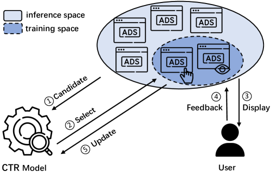
Figure 1. An illustration of the serving and updating process for CTR model in a typical online advertising system.

As shown in Fig. 1, a production CTR model scores all candidates and selects the top few based on Eq. (1) for display. The displayed ads as well as user feedback (i.e., click/non-click) are then recorded, with which we continuously train new models. Due to its simplicity and robustness, such a training paradigm is widely adopted by many industrial systems (Anil et al., 2022; Ma et al., 2022; Ling et al., 2017). However, since the displayed ads are not uniformly sampled from all candidates but purposely selected by the model itself, the training data distribution could be skewed from the inference distribution. This is widely known as the sample selection bias (SSB) problem  (Zadrozny, 2004; Heckman, 1979). It violates the classical assumption of training-inference consistency and may potentially affect the model performance.

Recent efforts (Wang et al., 2016; Ovaisi et al., 2020; Schnabel et al., 2016; Liu et al., 2020; Yuan et al., 2019) have been devoted to alleviating SSB in ranking systems. Methods based on Inverse Propensity Scoring (Schnabel et al., 2016; Ovaisi et al., 2020; Wang et al., 2016) recover the underlying distribution by re-weighting the training samples. Despite theoretical soundness, they require a propensity model that accurately estimates sample occurrence probability, which is difficult to learn in dynamic and complicated environments. Moreover, sample re-weighting may yield un-calibrated predictions that are problematic for ads CTR models (Yan et al., 2022). Another line of work collects uniform data via random policy, which helps train an unbiased imputation model for non-displayed items (Yuan et al., 2019) or guide the CTR model training via knowledge distillation (Liu et al., 2020). However, even small production traffic (e.g., 1%) of the uniform policy will severely cause degraded user experience and revenue loss, and the obtained uniform data of this magnitude is insufficient for training industrial models with billions of parameters. With these issues, we investigate how to mitigate SSB for industrial CTR models under a uniform-data-free framework.

Inspired by causal learning (Wang et al., 2020; Bonner and Vasile, 2018), CTR prediction can be framed as the problem of treatment effect estimation. As in Fig. 2(B), sample features compose unit $\mathbf{X}$, whether to display it acts as a binary treatment $\mathbf{T}$ and click is the outcome $\mathbf{Y}$ to estimate. The root cause of SSB is attributed to existence of confounders $\mathbf{\Delta}$ (e.g., item popularity) in $\mathbf{X}$ that affect both $\mathbf{T}$ and $\mathbf{Y}$. Recent studies (Hu et al., 2022; Geirhos et al., 2019) show that confounders mislead models to capture spurious correlations between the unit features and the outcome, which are non-causal and hurt generalization over the inference distribution. Hence, it is promising to mitigate SSB by disentangling confounders $\mathbf{\Delta}$ from real user-item interest $\mathbf{\Gamma}$ in sample features, which is non-trivial in absence of randomized controlled trials (i.e., uniform data) (Pearl, 2009).

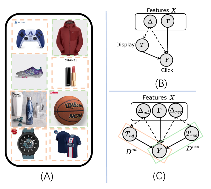
Figure 2. (A) Mixed results of ads (green dashed line) and recommendations (orange dashed line). (B,C) Causal Graph of CTR prediction for both ads and recommendations.

As shown in Fig. 2, many platforms (Chen et al., 2019; Goldfarb and Tucker, 2011) display mixed results of sponsored items and organic items that are independently selected by advertising and recommendation systems. For clarity, we refer to sponsored items as ads. We refer to organic items as recommendations. This scenario has two characteristics:

• Shared decision rationales. With a unified interface design, users are unaware of whether items are sponsored or organic, making their click decision determined by real user-item interest $\mathbf{\Gamma}$ rather than sources of displayed items.

• Different selection mechanisms. Advertising and recommendation systems serve different business targets (e.g., revenue/clicks/dwell time) (Goldfarb and Tucker, 2011) and have different selection mechanisms as verified in Sec. 2.2. Thus their SSB-related confounders are rarely overlapped, making system-specific confounders $\mathbf{\Delta_{ad}}$/$\mathbf{\Delta_{rec}}$ capture a substantial portion of $\mathbf{\Delta}$.

The above characteristics make it possible to disentangle $\mathbf{\Delta_{ad}}$/$\mathbf{\Delta_{rec}}$ and $\mathbf{\Gamma}$ by jointly considering samples from two sources. Compared with the uniform data, recommendation samples are of a comparable or even larger magnitude than ads samples and persist without revenue loss, making it a free lunch worthy of exploitation. Though few if any confounders common in two systems could still remain with $\mathbf{\Gamma}$, disentangling system-specific $\mathbf{\Delta_{ad}}$/$\mathbf{\Delta_{rec}}$ from $\mathbf{\Gamma}$ is already a meaningful step towards mitigating SSB, especially when uniform data is unavailable in industrial advertising systems.

To this end, we propose to leverage Recommendation samples to mitigate SSB For Ads CTR prediction (Rec4Ad). Under this framework, recommendation samples are retrieved and mixed with ad samples for training. With raw feature embeddings, we elaborately design the representation disentanglement mechanism to dissect system-specific confounders and system-invariant user-item interest across two systems. Specifically, this mechanism consists of an alignment module and a decorrelation module with various regularizations. Finally we make prediction with disentangled and enhanced representation. Rec4Ad has been deployed to serve the main traffic of Taobao display advertising system since July of 2022.

Our contributions are summarized as follows:

• We analyze the existence of SSB in CTR prediction and point out the potential to leverage recommendation samples to mitigate such bias in absence of uniform data.

• We propose a novel framework named Rec4Ad, which jointly considers the recommendation and ads samples in learning disentangled representations that dissect system-specific confounders and system-invariant user-item interest.

• We conduct offline and online experiments to validate the effectiveness of Rec4Ad that achieves substantial gains in business metrics (up to +6.6% CTR and +2.9% RPM).

2. Preliminary

2.1. Problem Formulation

Input: The input includes a user set $\mathbf{\mathcal{U}}$, an ad set $\mathbf{\mathcal{A}}$, an item set $\mathbf{\mathcal{I}}$, user-ad impressions $\mathbf{\mathcal{D}^{ad}}$, and user-item simpressions $\mathbf{\mathcal{D}^{rec}}$

• Each user $u\in\mathbf{\mathcal{U}}$ is represented by a set of features $\{u_{1},...,u_{m}\}$ including user profile features (e.g., age and gender) and historical behaviors (e.g., click and purchase).

• Each ad $a\in\mathbf{\mathcal{A}}$ is a promotion campaign for a sponsored item $i\in\mathbf{\mathcal{I}}$. Besides item-level features like category and brand, $a$ also has campaign-level features including ID and historical statistics, denoted by $\{a_{1},...,a_{n}\}$.

• Each impression in $D^{ad}$ is a tuple $(u,a,c,y)$ describing when the advertising system displayed $a$ to $u$ under context $c=\{c_{1},..,c_{k}\}$ such as time and device, user clicked it ($y=1$) or not ($y=0$). As for $D^{rec}$, the tuple changes to $(u,i,c,y)$ logged by the recommendation engine.

Output: We aim to learn a model $f$ that predicts the click probability $f(u,a,c)$ if displaying $a\in\mathbf{\mathcal{A}}$ to user $u\in\mathbf{\mathcal{U}}$ under context $c$.

2.2. Analysis of Sample Selection Bias

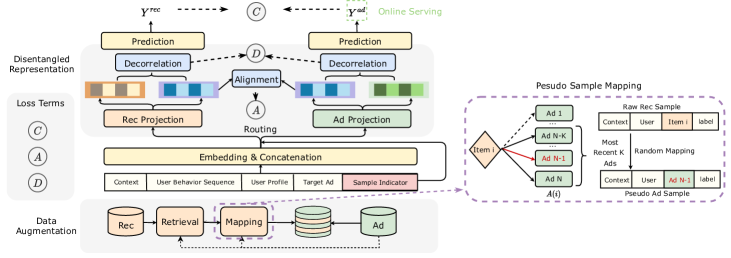
Figure 3. An overall framework of Rec4Ad (best viewed in color).

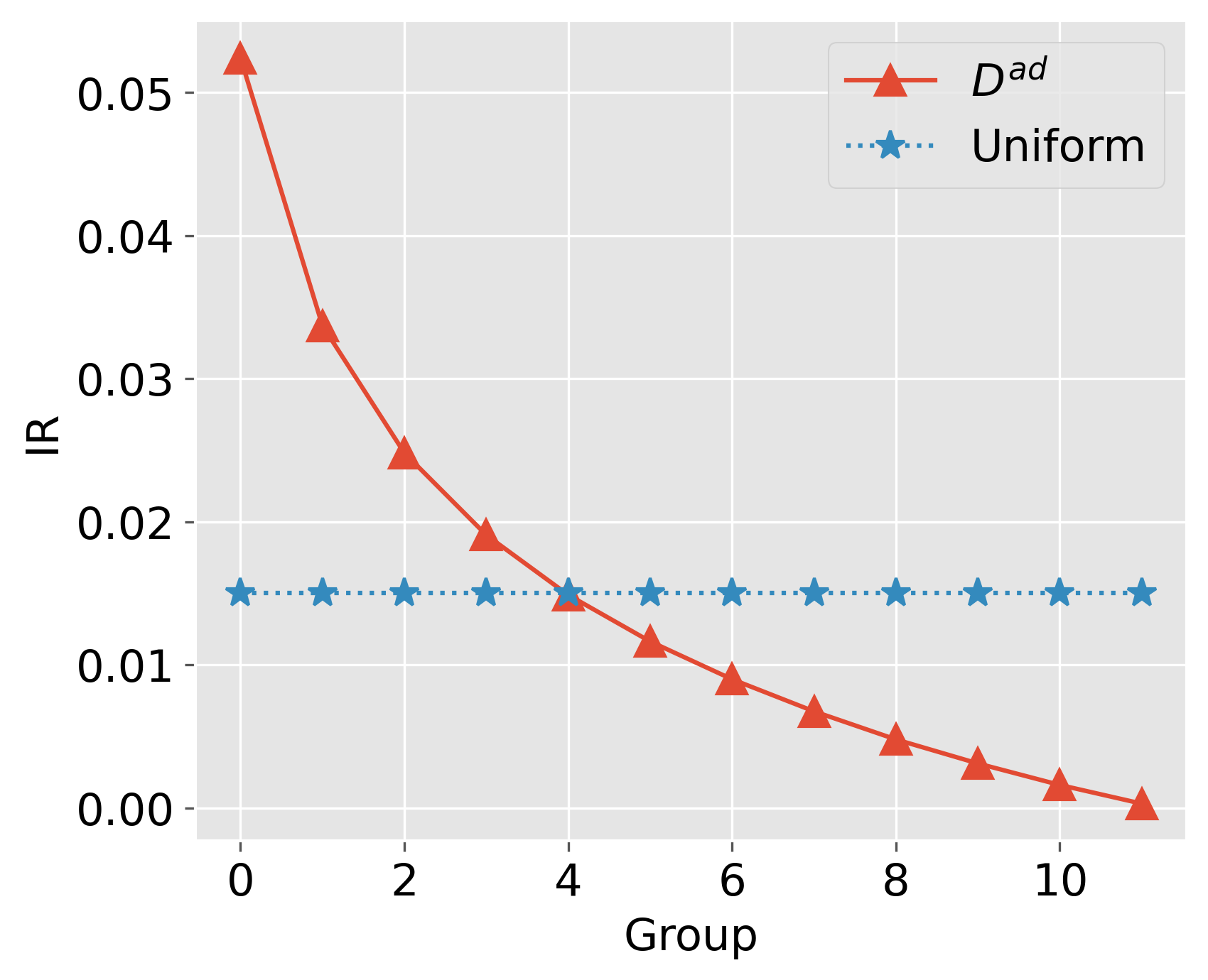
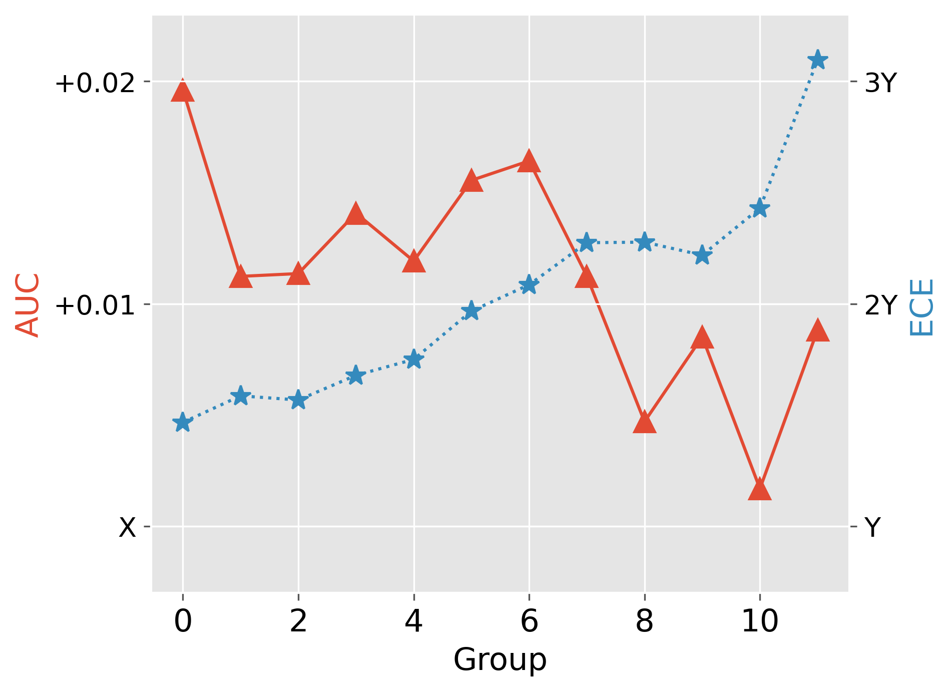
Figure 4. Left: Average IR for different groups of ads. Right: Model performance w.r.t different IR group of ads.

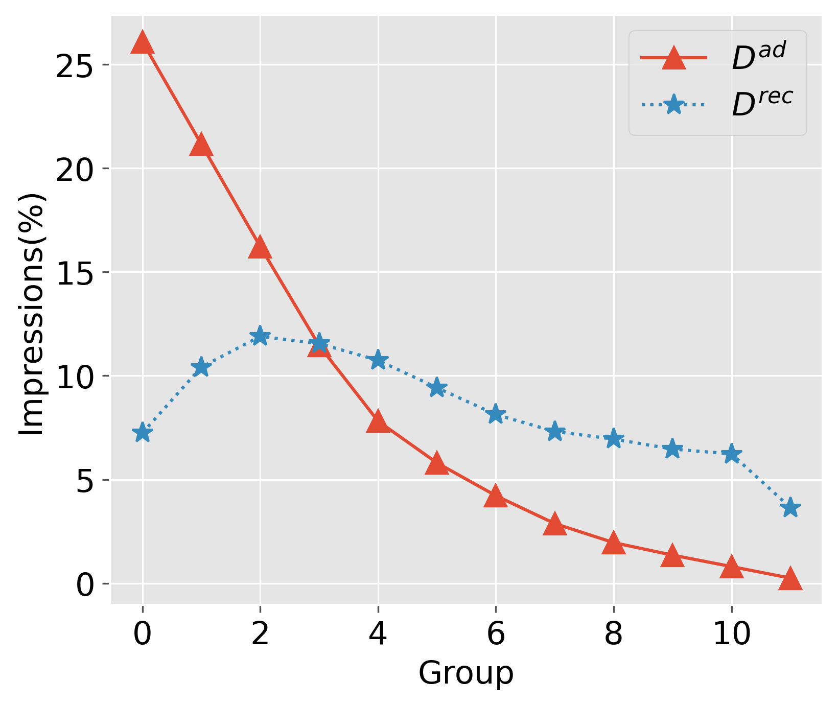
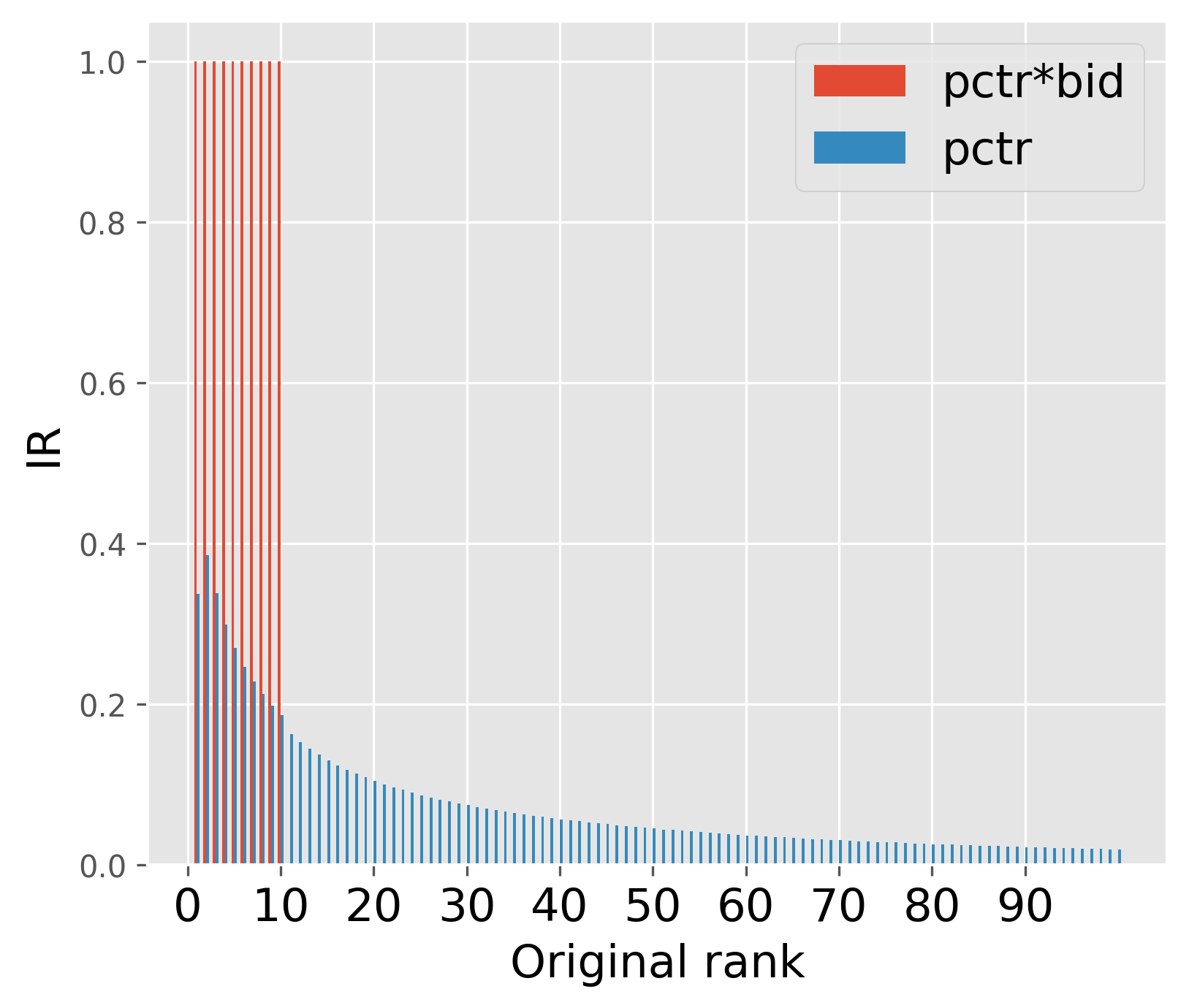
Figure 5. Left: Impression Distribution in $D^{ad}$ and $D^{rec}$. Right: Simulated results under different ranking mechanisms.

2.2.1. SSB in Ads Impressions

SSB happens when each candidate does not share equal opportunities for impression. To examine its existence, we define the metric of impression ratio (IR) to measure the opportunity of each ad in our system:

(2) $$\textbf{IR}(a)=\frac{\#\text{sessions where }a\text{ was displayed}}{\#\text{sessions where }a\text{ was in the candidate set}},$$

where a session refers to a user request. We first calculate IR for each ad in $D^{ad}$, sort them by IR in descending order, and then divide them equally into 12 groups. Fig. 4 (Left) shows the average IR for each group (the red line) compared with the ideal uniform data (the blue line). We find that impressions on $D^{ad}$ are distributed among different ads in an extremely imbalanced way, where the IR of the first group is nearly 200 times that of the last group.

2.2.2. Influence of SSB

Since base CTR model is trained on $D^{ad}$, we analyze its ranking and calibration performance under the imbalanced ad impressions. For ranking performance, we use the metric of AUC, and the calibration performance is measured by the Expected Calibration Error (ECE) (Yan et al., 2022). Details of two metrics are introduced in Sec. 4.1. Fig. 4 (Right) shows online model performance on different groups of ads with descending IR. It is observed that model tends to perform worse on ads with lower IR than on those with higher IR. It is consistent with our assumption that model does not generalize well on ads with few impressions and validates the necessity to handle SSB for improvement.

2.2.3. Mitigating SSB with Recommendation Samples.

As defined before, each ad in $\mathbf{\mathcal{A}}$ corresponds to an organic item in $\mathbf{\mathcal{I}}$. Thus we investigate how impressions in $D^{rec}$ are distributed among organic items with ad counterparts. From Fig. 5 (Left), we find that though some groups of ads have few impressions in $D^{ad}$, their corresponding items contribute an important portion of impressions in $D^{rec}$. It is attributed to different selection mechanism behind $D^{ad}$ and $D^{rec}$. We conduct a simulated study on $D^{ad}$ for verification, which changes the ranking function from $pctr*bid$ to $pctr$ (commonly adopted in recommendation systems) and re-displays top-10 ads. Fig. 5 (Right) illustrates IR of each original rank under two mechanisms. It is clear that impression distribution is changed, where ads with low rank in original list have opportunities to be displayed under another mechanism. Above empirical analysis show that it is promising to leverage recommendation samples in $D^{rec}$ to mitigate SSB in $D^{ad}$.

3. Methodology

Fig. 3 shows two stages of Rec4Ad in deployment: data augmentation and disentangled representation learning, which constructs and leverages recommendation (rec) samples, respectively.

3.1. Data Augmentation

3.1.1. Retrieving Recommendation Samples

To ensure user experience, the percentage of ad impressions in all impressions is usually limited to a low threshold. Typically, we have $|D^{ad}|\ll|D^{rec}|$, making it intractable to consume entire $D^{rec}$ owing to multiplied training resources. Moreover, not all rec samples are useful for enhancing ads model due to difference between $\mathbf{\mathcal{A}}$ and $\mathbf{\mathcal{I}}$. Thus we retrieve rec samples that are closely related to advertising system.

Let $I(a)\in\mathbf{\mathcal{I}}$ denote the item that $a\in\mathbf{\mathcal{A}}$ is advertised for. We define an item set $\mathbf{\mathcal{I}}^{ad}$ containing all items with related ads:

(3) $$\mathbf{\mathcal{I}}^{ad}=\{i\in\mathbf{\mathbf{I}}|\exists a\in\mathbf{\mathcal{A}},I(a)=i\}.$$

We discard rec samples whose items fail to occur in $\mathbf{\mathcal{I}}^{ad}$, since they fail to provide complementary impressions that relate to any ad of interest. In this way, we retrieve a subset of rec samples:

(4) $$D^{\hat{rec}}=\{(u,i,c,y)\in D^{rec}|i\in\mathbf{\mathcal{I}}^{ad}\}.$$

3.1.2. Pseudo Sample Mapping

The reasons to map retrieved rec samples to pseudo ad samples are two-fold. First, it allows rec samples and ad samples to have uniform input format, which facilitates efficient feature joining and batch processing. Second, pseudo samples scattering in the $\mathbf{\mathcal{U}}\times\mathbf{\mathcal{A}}$ space help learn a CTR prediction model for ads, compared with the $\mathbf{\mathcal{U}}\times\mathbf{\mathcal{I}}$ space.

In Fig. 3, we maintain an item-ads index where key is item $i$ and values are their related ads $A(i)=\{a\in\mathbf{\mathcal{A}}|I(a)=i\}$. To select an ad from $A(i)$, we do not take their impressions into consideration, which avoids introducing selection bias in the advertising system. Instead, we adopt a recent-$K$-random strategy. We randomly select an ad $a^{\prime}$ from most recent $K$ ads related to $i$, where $K$ is a fixed hyper-parameter. After mapping, we obtain the set of pseudo samples:

(5) $$D^{\tilde{rec}}=\{(u,a^{\prime},c,y)|(u,i,c,y)\in D^{\hat{rec}},a^{\prime}\in A(i)\},$$

3.2. Disentangled Representation Learning

3.2.1. Original Representation

we embed raw features of sample $(u,a,c,y)$ into low-dimensional vectors $[e(u),e(a),e(c)]$. Operations like attention mechanism (Zhou et al., 2018) are further employed to aggregate embeddings of user behavior sequences. We concatenate these results together to obtain intermediate representation $\mathbf{e}$.

Batch Normalization (BN) (Ioffe and Szegedy, 2015) is commonly used in training of industrial CTR models (Sheng et al., 2021) to stabilize convergence. It calculate statistics over training data for normalization during serving. However, when incorporating $D^{\tilde{rec}}$ into training, BN statistics are calculated based on ad and rec samples but only used to normalize ad samples during online serving. The distribution discrepancy between two kinds of samples weakens the effectiveness of BN.

To deal with this problem, we design source-aware BN (SABN), which adaptively normalize samples according to their sources. Let $s$ indicate which kind the sample is, SABN works as follows:

(6) $$SABN(e,s)=\gamma_{s}\frac{e-\mu_{s}}{\sqrt{\sigma_{s}^{2}+\epsilon}}+\beta_{s},s\in\{ad,rec\},\vspace{-2mm}$$

where $\gamma_{s},\beta_{s},\mu_{s},\sigma_{s}^{2}$ are source-specific parameters for normalization. Then we feed the normalized representation $\mathbf{e^{\prime}}$ into MLP (Multi-Layer Perception) layers for a compact representation $\mathbf{x}$ that captures feature interactions among user, ad, and context. We add superscripts on representations (e.g., $\mathbf{x}^{ad}$/$\mathbf{x}^{rec}$) to denote its source.

3.2.2. Alignment

Since users are usually unaware of the difference between ad and rec impressions, their click decisions can be assumed independent of underlying systems, which are commonly determined by their interest. To identify user-item interest $\mathbf{\Gamma}$ behind click decision, we propose to extract invariant representations shared between $D^{ad}$ and $D^{\tilde{rec}}$. In other words, samples in $D^{ad}$ and $D^{\tilde{rec}}$ should be indistinguishably distributed in the invariant representation space. To achieve this goal, we first apply projection layers over original representations of ad and rec samples:

(7) $$\mathbf{x}^{s}_{inv}=MLP^{s}_{inv}(\mathbf{x}^{s})\in\mathcal{R}^{d},s\in\{ad,rec\}$$

A direct method to align $\{\mathbf{x}^{ad}_{inv}\}$ and $\{\mathbf{x}^{rec}_{inv}\}$ is minimizing their Wasserstein or MMD distribution distance (Cuturi and Doucet, 2014; Gretton et al., 2012). However, these metrics are computationally inefficient and hard to estimate accurately over mini-batches. Instead, we train a sample discriminator $H$ to implicitly align them in an adversary way. Particularly, $H$ is a binary classifier that predicts whether the sample is from $D^{ad}$ or $D^{\tilde{rec}}$ based on $\mathbf{x}_{inv}$. Optimized with cross entropy loss, $H$ aims to distinguish two kinds of samples as accurate as possible:

(8) $$\hat{s}=Sigmoid(MLP_{H}(\mathbf{x}_{inv}^{s})),s\in\{ad,rec\},$$

$$L_{A}=-\sum_{D^{ad}}log(\hat{s})-\sum_{D^{\tilde{rec}}}log(1-\hat{s}).$$

While $H$ tries to minimize $L_{A}$ during training, neural layers generating invariant representations aim to make $\{\mathbf{x}^{ad}_{inv}\}$ and $\{\mathbf{x}^{rec}_{inv}\}$ indistinguishable as much as possible, i.e., maximize $L_{A}$. To train these two parts simultaneously, we insert a gradient reverse layer (GRL) (Ganin and Lempitsky, 2015) between $\mathbf{x}_{inv}$ and the discriminator. In forward propagation, GRL acts as an identity transformation. In backward propagation, it reverses gradients from subsequent layers:

(9) $$\text{Forward}:GRL(\mathbf{x}_{inv})=\mathbf{x}_{inv},$$

$$\text{Backward}:\frac{\partial L_{A}}{\partial\mathbf{x}_{inv}}=-\alpha\frac{\partial L_{A}}{\partial GRL(\mathbf{x}_{inv})},$$

where $\alpha$ controls the scale of reversion. In this way, we tightly align $\{\mathbf{x}^{ad}_{inv}\}$ and $\{\mathbf{x}^{rec}_{inv}\}$ in the invariant representation space.

3.2.3. Decorrelation

To separate system-specific confounders from original representation, we apply another set of projection layers:

(10) $$\mathbf{x}^{s}_{con} =MLP^{ad}_{con}(\mathbf{x}^{s})\in\mathcal{R}^{d},s\in\{ad,rec\}.$$

If without explicit constraints, $\mathbf{x}_{con}$ could still contain information shared across systems and prevent us from handling confounders specific to the ad system. To this end, we propose to add regularizations to further disentangle $\mathbf{x}_{con}$ and $\mathbf{x}_{inv}$.

Borrowing the idea that disentangled representations avoid encoding variations of each other (Cheung et al., 2014; Cogswell et al., 2015), we penalize the cross-correlation between two sets of representations. Specifically, let $\mathbf{p}_{i}$ denote the in-batch vector of $i$-th dimension of $\mathbf{x}_{inv}$ and $\mathbf{q}_{j}$ denote that of $j$-th dimension of $\mathbf{x}_{con}$, their Pearson correlation can be calculated as:

(11) $$Cov(\mathbf{p}_{i},\mathbf{q}_{j}))=[\mathbf{p}_{i}-\mathbf{\bar{p}_{i}}]^{\top}[\mathbf{q}_{j}-\mathbf{\bar{q}_{j}}],$$

$$\Upsilon(\mathbf{p}_{i},\mathbf{q}_{j})=\frac{Cov(\mathbf{p}_{i},\mathbf{q}_{j})}{\sqrt{Cov(\mathbf{p}_{i},\mathbf{p}_{i})}},$$

where $\mathbf{\bar{p}_{i}}$ and $\mathbf{\bar{q}_{j}}$ denote in-batch mean of each dimension. Thus the objective of the decorrelation module are based on correlations of every pair of dimension cross $\mathbf{x}_{inv}$ and $\mathbf{x}_{con}$:

(12) $$L_{D}=\sum_{i=1}^{d}\sum_{j=1}^{d}[\Upsilon(\mathbf{p}^{ad}_{i},\mathbf{q}^{ad}_{j})^{2}+\Upsilon(\mathbf{p}^{rec}_{i},\mathbf{q}^{rec}_{j})^{2}].$$

By optimizing $L_{D}$, $\mathbf{x}_{con}$ are encouraged to capture residual information independent from $\mathbf{x}_{inv}$, i.e., system-specific confounders $\mathbf{\Delta_{ad}}$/$\mathbf{\Delta_{rec}}$ that are discarded by the alignment module.

3.3. Prediction

We reconstruct final representation based on disentangled representations to predict CTR. Previous studies show that non-causal associations also potentially contribute to prediction accuracy (Zhang et al., 2021; Si et al., 2022), motivating us to consider $\mathbf{x}_{con}$ in reconstruction instead of directly ignoring it. For simplicity, we use the concatenation operator:

(13) $$\mathbf{x}^{s}_{new}=\mathbf{x}^{s}_{inv}\oplus\mathbf{x}^{s}_{con},s\in\{ad,rec\}.$$

With $\mathbf{x}_{new}^{s}$, we make predictions for ad samples and pseudo samples with source-aware layers, where cross entropy loss $L_{C}$ is optimized:

(14) $$\hat{y}^{s}=Sigmoid(MLP^{s}_{pred}(\mathbf{x}^{s}_{new})),s\in\{ad,rec\}$$

$$L_{C}=\sum_{D^{ad}\cup D^{\tilde{rec}}}[-ylog(\hat{y}^{s})-(1-y)log(1-\hat{y}^{s})].$$

Thus the objective function of Rec4Ad consists of the CTR prediction loss, the alignment loss and the decorrelation loss:

(15) $$L=L_{C}+\lambda_{1}L_{A}+\lambda_{2}L_{D}.$$

4. Experiments

4.1. Experimental Setup

Taobao Production Dataset. We construct the dataset based on impression logs in two weeks of 2022/06 from Taobao advertising system and recommendation system. We use data of the first week for training, which contains ad and rec impressions collected under regular policy. The data of the next week are ad impressions collected under random policy of a small traffic following (Yuan et al., 2019; Liu et al., 2020), which is used to evaluate model performance against SSB. The training dataset contains 1.9 billion ad samples and 0.6 billion rec samples after retrieval, covering 0.2 billion users. The test dataset contains 18.9 million ad samples and 10.3 million users.

Baselines. Rec4Ad is compared with following baselines.

• Base. We adopt DIN (Zhou et al., 2018) as the vanilla model which does not account for SSB.

• DAG. The Data-Augmentation (DAG) method directly merges rec samples and ad samples to train the base model.

• IPS (Joachims et al., 2017; Schnabel et al., 2016). It eliminates SSB by re-weighting samples with inverse propensity of ad impression.

• IPS-C (Bottou et al., 2013) It adds max-capping to IPS weight so that its variance can be reduced.

• IV (Si et al., 2022). It employs user behaviors outside current system as instrumental variables for model debiasing.

Metrics. For ranking ability, we use the standard AUC (Area Under the ROC Curve) metric for evaluation (Lian et al., 2018; Guo et al., 2017). A higher AUC indicates better ranking performance. In practice, absolute improvement of AUC by 0.001 on the production dataset is considered significant, which empirically leads to an online lift of 1% CTR. For calibration, we evaluate models with the ECE (Yan et al., 2022) metric. We first equally partition the $pctr$ range [0,1] into $K$ buckets $B_{1},...,B_{K}$. ECE can be calculated as follows:

(16) $$\text{ECE}=\frac{1}{|D|}\sum_{k=1}^{K}|\sum_{i=1}^{|D|}(y_{i}-\hat{y}_{i})\>\vmathbb{1}(\hat{y}_{i}\in{B_{k}})|,$$

where $\vmathbb{1}(\hat{y}_{i}\in{B_{k}})$ equals 1 only if $\hat{y}_{i}\in{B_{k}}$ else 0. $K$ is set to 100. A lower ECE here indicates better calibration performance.

Implementation The feature embedding size is 16. We use Adam optimizer (Kingma and Ba, 2014) with initial learning rate $0.001$. The batch size is fixed to 6000. In data augmentation, we consider the most recent 3 ads for pseudo sample mapping. The dimensions $d$ of $\mathbf{x}_{inv}$ and $\mathbf{x}_{con}$ is 128. The ratio $\alpha$ of gradient reverse layer in Eq. (9) is 0.1. $\lambda_{1}$ and $\lambda_{2}$ for the alignment and the decorrelation loss in Eq. (15) is 0.005 and 0.5. For tests of significance, each experiment is repeated 5 times by random initialization and we report the average as results.

4.2. Experimental Results

Table 1. Performance Comparison of Rec4Ad and baselines. The symbol * indicates the improvements over baselines are significant with p-value ¡ 0.01 by t-test. We omit standard deviations since they are all no more than $2\times 10^{-4}$.

Method	AUC	Impv.	ECE	Impv.
Base	0.6778	-	0.0007	-
DAG	0.6724	-0.0054	0.0032	-0.0025
IPS	0.6618	-0.0160	0.0023	-0.0016
IPS-C	0.6783	+0.0005	0.0015	-0.0008
IV	0.6790	+0.0012	0.0009	-0.0002
Rec4Ad	0.6805*	+0.0027	0.0002	+0.0005

4.2.1. Overall Performance

From Table 1, we find that Rec4Ad significantly performs better than all baselines. Specifically, it outperforms Base in terms of AUC by 0.0027 and outperforms the state-of-the-art IV by 0.0015. This demonstrates the effectiveness of our proposed framework in handling SSB. By dissecting confounders and user-item interest for enhanced representations, it works well over the inference space. Moreover, Rec4Ad successfully maintains even slightly better model calibration than Base, which also verifies its suitability for ads CTR prediction. We also observe that DAG performs worse than baseline both in AUC and ECE. The reason is ad samples and rec samples present different feature distributions and label distributions. Naive data augmentation actually amplifies the distribution discrepancy between training and inference. The original IPS yields worst AUC, while IPS-C with max-capping achieves higher AUC than Base. We attribute this phenomenon to high variance in estimation of propensity score. We also notice that ECE of IPS and IPS-C are all larger than $10^{-3}$, which verifies that sample re-weighting could change label distribution and result in calibration issues of ads CTR prediction.

4.2.2. Performance on Different Ad Groups

Table 2. Comparison among Rec4Ad and three competitive baselines on ad groups with different impression ratios.

Group	Method	AUC	Impv.	ECE	Impv.
$G_{top}$	Base	0.6741	-	0.0002	-
	IPS-C	0.6736	-0.0005	0.0004	-0.0002
	IV	0.6743	+0.0002	0.0002	0
	Rec4Ad	0.6757*	+0.0016	0.0002	0
$G_{bottom}$	Base	0.6625	-	0.0021	-
	IPS-C	0.6648	+0.0023	0.0018	+0.0003
	IV	0.6734	+0.0009	0.0021	0
	Rec4Ad	0.6654*	+0.0029	0.0010*	+0.0011

In Section 2.2.2, we show that SSB leads model to perform badly on ads with low impression ratios. To validate whether Rec4Ad mitigates such influence, we compare Rec4Ad and three competitive baselines on specific ad groups. We sort ads in descending IR as defined in Eq. (2), where the top 25% are selected as $G_{top}$ representing ads with enough impressions and the bottom 25% are selected as $G_{bottom}$ containing ads that are less represented in the training data.

Table 2 shows that Rec4Ad achieves best ranking and calibration performance on both $G_{top}$ and $G_{bottom}$. The improvements over Base are greater on $G_{bottom}$ with AUC increased by nearly 0.003 and ECE reduced by 0.001. Thus we conclude that Rec4Ad succeeds in mitigating SSB and boosts model performance on those long-tail ads. We also observe an interesting seesaw phenomenon about IPS-C, which also greatly improves metrics on $G_{bottom}$ but yields worse performance on $G_{top}$ compared with Base. It is because IPS-C explicitly imposes higher weights for samples with low-IR ads and lower weights for those with high-IR ads. By contrast, Rec4Ad exhibits its superiority that improvements on $G_{bottom}$ are achieved without the cost of degraded performance on $G_{top}$.

4.2.3. Ablation Study

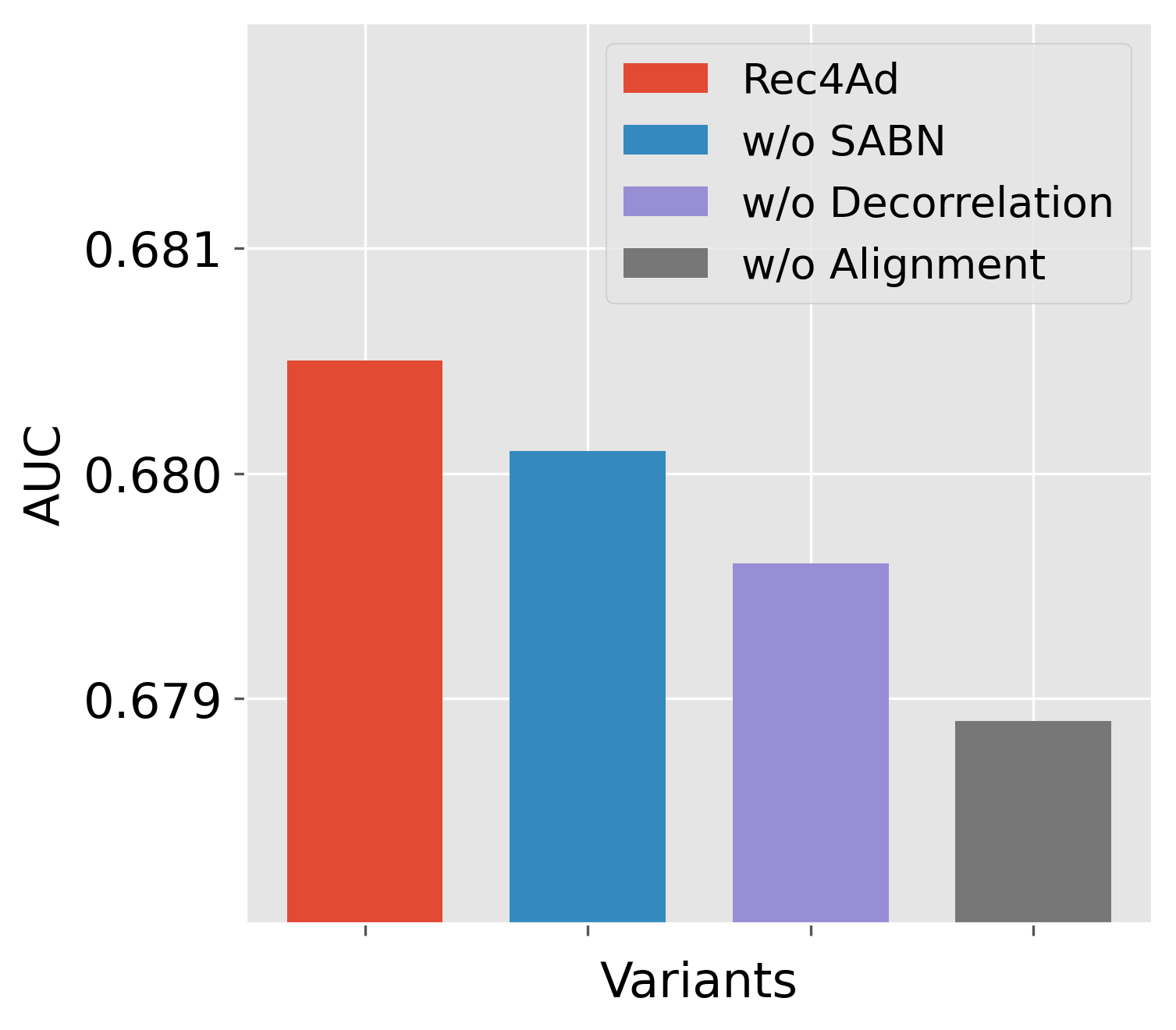
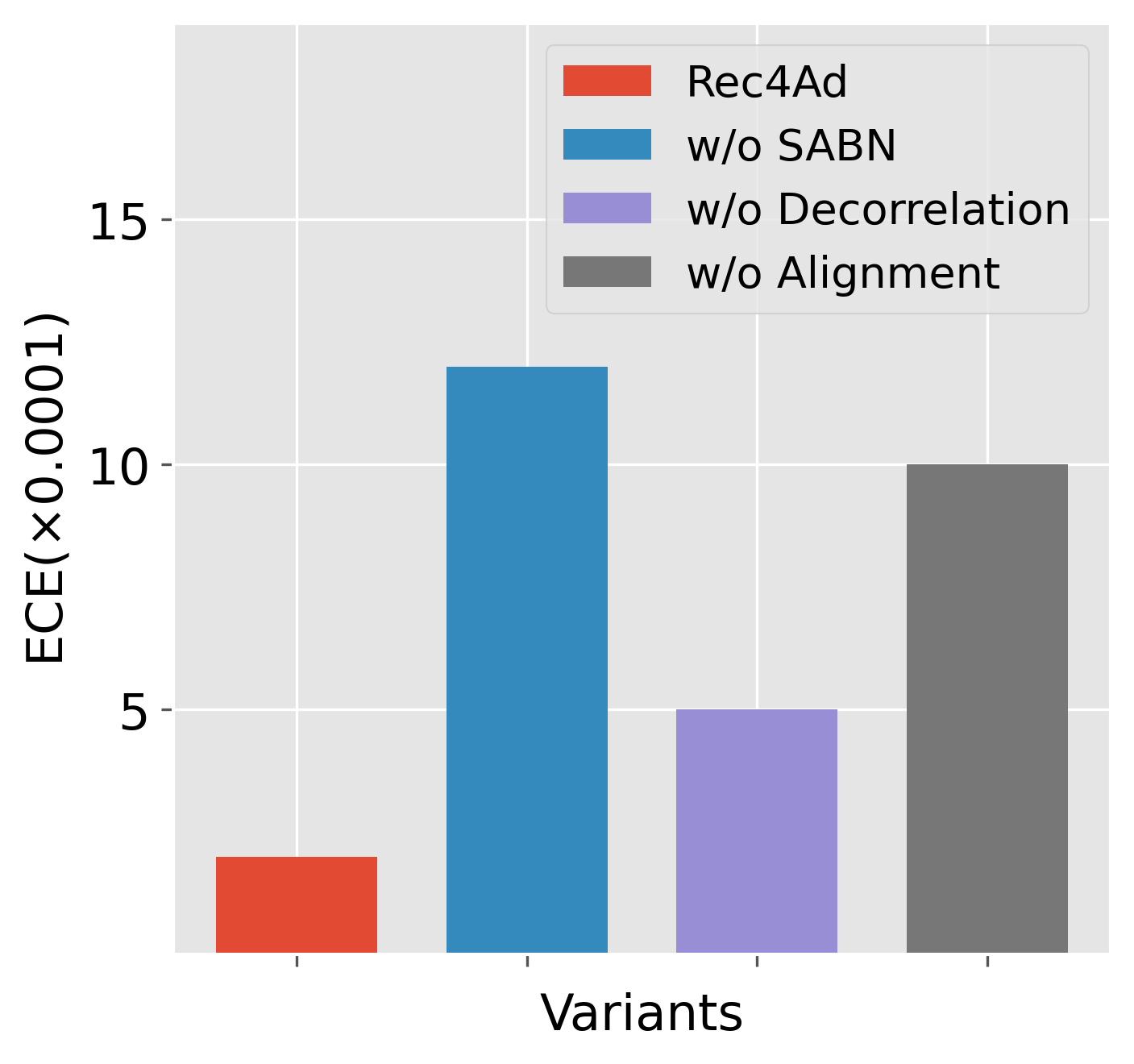
Figure 6. Comparison among Rec4Ad and its variants.

We analyze the effect of key components in Rec4Ad by comparing it with variants which remove SABN, the alignment module, and the decorrelation module, respectively.

Fig. 6 shows that after removing SABN, model calibration experiences an obvious degeneration. The reason is that representations of Rec and Ad samples are with different distributions, making it difficult to normalize them with shared BN parameters and leading to mis-scaled network activations as well as badly-calibrated predictions. Furthermore, we find that AUC even drops under $0.679$ after removing the alignment module, validating that the alignment regularization is critical for co-training with ad and rec samples. It allows Rec4Ad to extract shared user-item interest behind user clicks and eliminate system-specific confounders from this part. The decorrelation module is also shown effective since the variant without this component performs worse than the default version. It is because splitting non-causal correlations alone in enhanced representations also potentially contributes to accurate predictions (Zhang et al., 2021; Si et al., 2022).

4.2.4. Study on Disentangled Representations

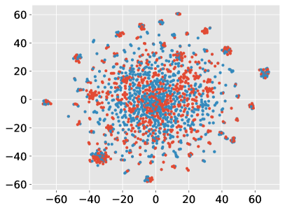
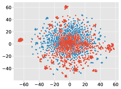
Figure 7. T-SNE visualization of $\mathbf{x}_{inv}$ (Left) and $\mathbf{x}_{con}$ (Right) for ad samples (red) and rec samples (blue).

Figure 8. Training AUC of the adversary sample classifier $H$.

As $\mathbf{x}_{inv}$ and $\mathbf{x}_{con}$ are expected to capture system-invariant and system-specific factors respectively, we aim to investigate their distributions over ad and rec samples. We randomly sample a hybrid batch and visualize learned representations using t-SNE (Van der Maaten and Hinton, 2008). As shown in Fig. 7, there is no significant difference between $\mathbf{x}_{inv}$ for ad and rec samples, suggesting the captured invariance. When it comes to $\mathbf{x}_{con}$, we observe that ad samples and rec samples are mostly separated in different areas, indicating that this representation extracts system-specific factors from the training data, which we believe stems from the difference in their selection mechanisms.

In the alignment module, we employs an adversary sample discriminator $H$ to distinguish $\mathbf{x}_{inv}^{ad}$ and $\mathbf{x}_{inv}^{rec}$. Thus the classification performance can be used as an effective proxy to quantitatively evaluate the goodness of $\mathbf{x}_{inv}$. Fig. 8 illustrates the adversary AUC during training. We observe that it increases at the early stage due to optimization of $H$. Then AUC gradually decreases as the training goes on, indicating Rec4Ad tries to generate representations that confuse $H$. Near the end of training, AUC converges to 0.5, which means ad and rec samples are indistinguishable on $\mathbf{x}_{inv}$.

4.3. Online Study

Table 3. Key business metrics of online A/B Test.

Scene	Overall		Long-Tail
	CTR	RPM	CTR	RPM
Homepage	+6.6%	+2.9%	+12.6%	+9.3%
Post-Purchase	+3.0%	+2.6%	+3.6%	+0.8%

We conduct online A/B Test between Rec4Ad and production baseline from July 1 to July 7 of 2022, each with 5% randomly-assigned traffic. Two key business metrics are used in evaluation: Click-Through Rate (CTR) and Revenue Per Mille (RPM), which corresponds to user experience and platform revenue, respectively. As shown in Table 3, Rec4Ad achieves substantial gains in two largest scenes of Taobao display advertising business, Homepage and Post-Purchase, demonstrating considerable business value of Rec4Ad. For long-tail ads with few impressions. Rec4Ad achieves up to 12.6% and 3.6% lift of CTR in two scenes, which are larger than the overall lift. Above results verify that Rec4Ad effectively mitigates SSB and brings solid online improvements. It has been successfully deployed in production environment to serve the main traffic of Taobao display advertising system since July of 2022.

5. Conclusion

In this paper, we propose a novel framework which leverages Recommendation samples to help mitigate sample selection bias For Ads CTR prediction (Rec4Ad). Recommendation samples are first retrieved and mapped to pseudo samples. Ad samples and pseudo samples are jointly considered in learning disentangled representations that dissect system-specific confounders brought by selection mechanisms and system-invariant user-item interest. Alignment and decorrelation modules are included in above architecture. When deployed in Taobao display advertising system, Rec4Ad achieves substantial gains in key business metrics, with a lift of up to +6.6% CTR and +2.9% RPM.

References

- (1)
- Anil et al. (2022) Rohan Anil, Sandra Gadanho, Da Huang, Nijith Jacob, Zhuoshu Li, Dong Lin, Todd Phillips, Cristina Pop, Kevin Regan, Gil I Shamir, et al. 2022. On the Factory Floor: ML Engineering for Industrial-Scale Ads Recommendation Models. arXiv preprint arXiv:2209.05310 (2022).
- Bonner and Vasile (2018) Stephen Bonner and Flavian Vasile. 2018. Causal Embeddings for Recommendation. In Proceedings of the 12th ACM conference on recommender systems. Association for Computing Machinery, New York, NY, USA, 104–112.
- Bottou et al. (2013) Léon Bottou, Jonas Peters, Joaquin Quiñonero-Candela, Denis X Charles, D Max Chickering, Elon Portugaly, Dipankar Ray, Patrice Simard, and Ed Snelson. 2013. Counterfactual Reasoning and Learning Systems: The Example of Computational Advertising. Journal of Machine Learning Research 14, 11 (2013).
- Chen et al. (2019) Dagui Chen, Junqi Jin, Weinan Zhang, Fei Pan, Lvyin Niu, Chuan Yu, Jun Wang, Han Li, Jian Xu, and Kun Gai. 2019. Learning to Advertise for Organic Traffic Maximization in E-Commerce Product Feeds. In Proceedings of the 28th ACM International Conference on Information and Knowledge Management. 2527–2535.
- Cheung et al. (2014) Brian Cheung, Jesse A Livezey, Arjun K Bansal, and Bruno A Olshausen. 2014. Discovering hidden factors of variation in deep networks. arXiv preprint arXiv:1412.6583 (2014).
- Cogswell et al. (2015) Michael Cogswell, Faruk Ahmed, Ross Girshick, Larry Zitnick, and Dhruv Batra. 2015. Reducing overfitting in deep networks by decorrelating representations. arXiv preprint arXiv:1511.06068 (2015).
- Cuturi and Doucet (2014) Marco Cuturi and Arnaud Doucet. 2014. Fast computation of Wasserstein barycenters. In International conference on machine learning. PMLR, 685–693.
- Ganin and Lempitsky (2015) Yaroslav Ganin and Victor Lempitsky. 2015. Unsupervised domain adaptation by backpropagation. In International conference on machine learning. PMLR, 1180–1189.
- Geirhos et al. (2019) Robert Geirhos, Patricia Rubisch, Claudio Michaelis, Matthias Bethge, Felix A. Wichmann, and Wieland Brendel. 2019. ImageNet-trained CNNs are biased towards texture; increasing shape bias improves accuracy and robustness.. In International Conference on Learning Representations. https://openreview.net/forum?id=Bygh9j09KX
- Goldfarb and Tucker (2011) Avi Goldfarb and Catherine Tucker. 2011. Online display advertising: Targeting and obtrusiveness. Marketing Science 30, 3 (2011), 389–404.
- Gretton et al. (2012) Arthur Gretton, Karsten M Borgwardt, Malte J Rasch, Bernhard Schölkopf, and Alexander Smola. 2012. A kernel two-sample test. The Journal of Machine Learning Research 13, 1 (2012), 723–773.
- Guo et al. (2017) Huifeng Guo, Ruiming Tang, Yunming Ye, Zhenguo Li, and Xiuqiang He. 2017. DeepFM: a factorization-machine based neural network for CTR prediction. arXiv preprint arXiv:1703.04247 (2017).
- Heckman (1979) James J Heckman. 1979. Sample selection bias as a specification error. Econometrica: Journal of the econometric society (1979), 153–161.
- Hu et al. (2022) Ziniu Hu, Zhe Zhao, Xinyang Yi, Tiansheng Yao, Lichan Hong, Yizhou Sun, and Ed H. Chi. 2022. Improving Multi-Task Generalization via Regularizing Spurious Correlation. In Advances in Neural Information Processing Systems, Alice H. Oh, Alekh Agarwal, Danielle Belgrave, and Kyunghyun Cho (Eds.). https://openreview.net/forum?id=HLzjd09oRx
- Ioffe and Szegedy (2015) Sergey Ioffe and Christian Szegedy. 2015. Batch normalization: Accelerating deep network training by reducing internal covariate shift. In International conference on machine learning. pmlr, 448–456.
- Joachims et al. (2017) Thorsten Joachims, Adith Swaminathan, and Tobias Schnabel. 2017. Unbiased learning-to-rank with biased feedback. In Proceedings of the tenth ACM international conference on web search and data mining. 781–789.
- Kingma and Ba (2014) Diederik P Kingma and Jimmy Ba. 2014. Adam: A method for stochastic optimization. arXiv preprint arXiv:1412.6980 (2014).
- Lian et al. (2018) Jianxun Lian, Xiaohuan Zhou, Fuzheng Zhang, Zhongxia Chen, Xing Xie, and Guangzhong Sun. 2018. xdeepfm: Combining explicit and implicit feature interactions for recommender systems. In Proceedings of the 24th ACM SIGKDD international conference on knowledge discovery & data mining. 1754–1763.
- Ling et al. (2017) Xiaoliang Ling, Weiwei Deng, Chen Gu, Hucheng Zhou, Cui Li, and Feng Sun. 2017. Model ensemble for click prediction in bing search ads. In Proceedings of the 26th international conference on world wide web companion. 689–698.
- Liu et al. (2020) Dugang Liu, Pengxiang Cheng, Zhenhua Dong, Xiuqiang He, Weike Pan, and Zhong Ming. 2020. A General Knowledge Distillation Framework for Counterfactual Recommendation via Uniform Data. In Proceedings of the 43rd International ACM SIGIR Conference on Research and Development in Information Retrieval. Association for Computing Machinery, 831–840.
- Ma et al. (2022) Ning Ma, Mustafa Ispir, Yuan Li, Yongpeng Yang, Zhe Chen, Derek Zhiyuan Cheng, Lan Nie, and Kishor Barman. 2022. An Online Multi-task Learning Framework for Google Feed Ads Auction Models. In Proceedings of the 28th ACM SIGKDD Conference on Knowledge Discovery and Data Mining. 3477–3485.
- Ovaisi et al. (2020) Zohreh Ovaisi, Ragib Ahsan, Yifan Zhang, Kathryn Vasilaky, and Elena Zheleva. 2020. Correcting for selection bias in learning-to-rank systems. In Proceedings of The Web Conference 2020. 1863–1873.
- Pearl (2009) Judea Pearl. 2009. Causality. Cambridge university press.
- Schnabel et al. (2016) Tobias Schnabel, Adith Swaminathan, Ashudeep Singh, Navin Chandak, and Thorsten Joachims. 2016. Recommendations as Treatments: Debiasing Learning and Evaluation. In Proceedings of The 33rd International Conference on Machine Learning (Proceedings of Machine Learning Research, Vol. 48). PMLR, 1670–1679.
- Sheng et al. (2021) Xiang-Rong Sheng, Liqin Zhao, Guorui Zhou, Xinyao Ding, Binding Dai, Qiang Luo, Siran Yang, Jingshan Lv, Chi Zhang, Hongbo Deng, et al. 2021. One model to serve all: Star topology adaptive recommender for multi-domain ctr prediction. In Proceedings of the 30th ACM International Conference on Information & Knowledge Management. 4104–4113.
- Si et al. (2022) Zihua Si, Xueran Han, Xiao Zhang, Jun Xu, Yue Yin, Yang Song, and Ji-Rong Wen. 2022. A model-agnostic causal learning framework for recommendation using search data. In Proceedings of the ACM Web Conference 2022. 224–233.
- Van der Maaten and Hinton (2008) Laurens Van der Maaten and Geoffrey Hinton. 2008. Visualizing data using t-SNE. Journal of machine learning research 9, 11 (2008).
- Wang et al. (2016) Xuanhui Wang, Michael Bendersky, Donald Metzler, and Marc Najork. 2016. Learning to rank with selection bias in personal search. In Proceedings of the 39th International ACM SIGIR conference on Research and Development in Information Retrieval. 115–124.
- Wang et al. (2020) Yixin Wang, Dawen Liang, Laurent Charlin, and David M Blei. 2020. Causal inference for recommender systems. In Fourteenth ACM Conference on Recommender Systems. 426–431.
- Yan et al. (2022) Le Yan, Zhen Qin, Xuanhui Wang, Michael Bendersky, and Marc Najork. 2022. Scale Calibration of Deep Ranking Models. In Proceedings of the 28th ACM SIGKDD Conference on Knowledge Discovery and Data Mining. 4300–4309.
- Yuan et al. (2019) Bowen Yuan, Jui-Yang Hsia, Meng-Yuan Yang, Hong Zhu, Chih-Yao Chang, Zhenhua Dong, and Chih-Jen Lin. 2019. Improving ad click prediction by considering non-displayed events. In Proceedings of the 28th ACM International Conference on Information and Knowledge Management. 329–338.
- Zadrozny (2004) Bianca Zadrozny. 2004. Learning and evaluating classifiers under sample selection bias. In Proceedings of the twenty-first international conference on Machine learning. 114.
- Zhang et al. (2021) Yang Zhang, Fuli Feng, Xiangnan He, Tianxin Wei, Chonggang Song, Guohui Ling, and Yongdong Zhang. 2021. Causal intervention for leveraging popularity bias in recommendation. In Proceedings of the 44th International ACM SIGIR Conference on Research and Development in Information Retrieval. 11–20.
- Zhou et al. (2018) Guorui Zhou, Xiaoqiang Zhu, Chenru Song, Ying Fan, Han Zhu, Xiao Ma, Yanghui Yan, Junqi Jin, Han Li, and Kun Gai. 2018. Deep interest network for click-through rate prediction. In Proceedings of the 24th ACM SIGKDD international conference on knowledge discovery & data mining. 1059–1068.