Instructive Feature Enhancement for Dichotomous Medical Image Segmentation

Abstract

Deep neural networks have been widely applied in dichotomous medical image segmentation (DMIS) of many anatomical structures in several modalities, achieving promising performance. However, existing networks tend to struggle with task-specific, heavy and complex designs to improve accuracy. They made little instructions to which feature channels would be more beneficial for segmentation, and that may be why the performance and universality of these segmentation models are hindered. In this study, we propose an instructive feature enhancement approach, namely IFE, to adaptively select feature channels with rich texture cues and strong discriminability to enhance raw features based on local curvature or global information entropy criteria. Being plug-and-play and applicable for diverse DMIS tasks, IFE encourages the model to focus on texture-rich features which are especially important for the ambiguous and challenging boundary identification, simultaneously achieving simplicity, universality, and certain interpretability. To evaluate the proposed IFE, we constructed the first large-scale DMIS dataset Cosmos55k, which contains 55,023 images from 7 modalities and 26 anatomical structures. Extensive experiments show that IFE can improve the performance of classic segmentation networks across different anatomies and modalities with only slight modifications. Code is available at https://github.com/yezi-66/IFE

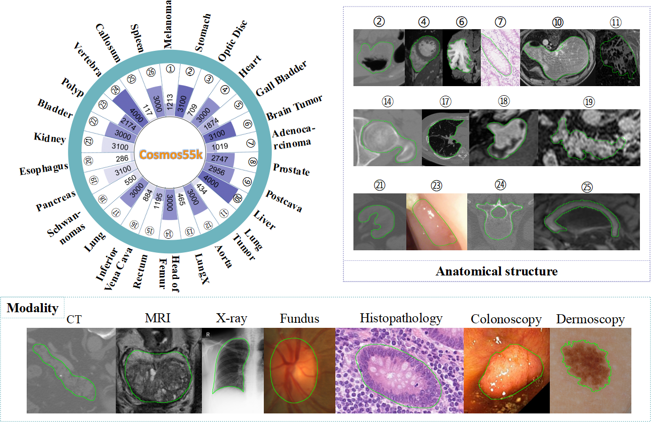
Figure 1: Statistics, modalities, and examples of anatomical structures in Cosmos55k.

1 Introduction

Medical image segmentation (MIS) can provide important information regarding anatomical or pathological structural changes and plays a critical role in computer-aided diagnosis. With the rapid development of intelligent medicine, MIS involves an increasing number of imaging modalities, raising requirements for the accuracy and universality of deep models.

Medical images have diverse modalities owing to different imaging methods. Images from the same modality but various sites can exhibit high similarity in overall structure but diversity in details and textures. Models trained on specific modalities or anatomical structure datasets may not adapt to new datasets. Similar to dichotomous image segmentation tasks [26], MIS tasks typically input an image and output a binary mask of the object, which primarily relies on the dataset. To facilitate such dichotomous medical image segmentation (DMIS) task, we constructed Cosmos55k, a large-scale dataset of 55,023 challenging medical images covering 26 anatomical structures and 7 modalities (see Fig. 1).

Most current MIS architectures are carefully designed. Some increased the depth or width of the backbone network, such as UNet++ [36], which uses nested and dense skip connections, or DeepLabV3+ [9], which combines dilated convolutions and feature pyramid pooling with an effective decoder module. Others have created functional modules such as Inception and its variants [31, 10], depthwise separable convolution [17], attention mechanism [16, 33], and multi-scale feature fusion [8]. Although these modules are promising and can be used flexibly, they typically require repeated and handcrafted adaptation for diverse DMIS tasks. Alternatively, frameworks like nnUNet [18] developed an adaptive segmentation pipeline for multiple DMIS tasks by integrating key dataset attributes and achieved state-of-the-art. However, heavy design efforts are needed for nnUNet and the cost is very expensive. More importantly, previous DMIS networks often ignored the importance of identifying and enhancing the determining and instructive feature channels for segmentation, which potentially limits their performance in general DMIS tasks.

We observed that the texture-rich and sharp-edge cues in specific feature channels are crucial and instructive for accurately segmenting objects. Curvature [15] can represent the edge characteristics in images. Information entropy [1] can describe the texture and content complexity of images. In this study, we focus on exploring their roles in quantifying feature significance. Based on curvature and information entropy, we propose a simple approach to balance accuracy and universality with only minor modifications of the classic networks. Our contribution is three folds. First, we propose the novel 2D DMIS task and construct a large-scale dataset (Cosmos55k) to benchmark the goal and we will release the dataset to contribute to the community. Second, we propose a simple, generalizable, and effective instructive feature enhancement approach (IFE). With extensive experiments on Cosmos55k, IFE soundly proves its advantages in promoting various segmentation networks and tasks. Finally, we provide an interpretation of which feature channels are more beneficial to the final segmentation results. We believe IFE will benefit various DMIS tasks.

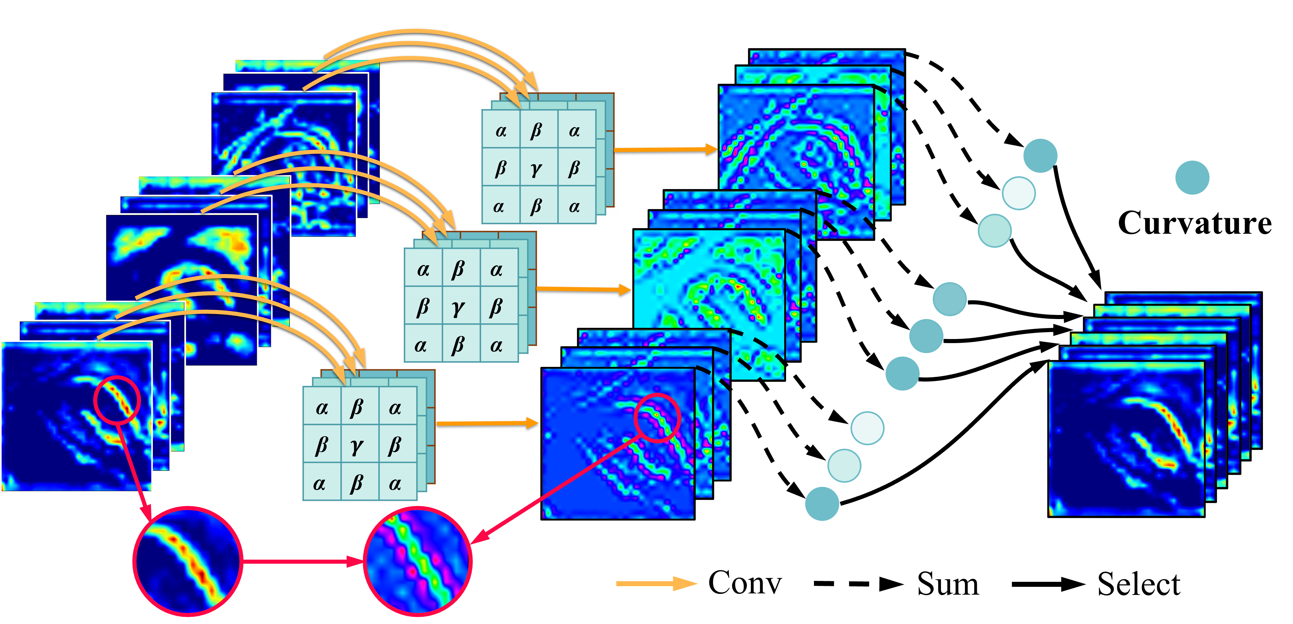
Figure 2: Example of feature selection using curvature.

2 Methodology

Overview. Fig. 2 and Fig. 3 illustrate two choices of the proposed IFE. It is general for different DMIS tasks. 1) We introduce a feature quantization method based on either curvature (Fig. 2) or information entropy (Fig. 3), which characterizes the content abundance of each feature channel. The larger these parameters, the richer the texture and detail of the corresponding channel feature. 2) We select a certain proportion of channel features with high curvature or information entropy and combine them with raw features. IFE improves performance with minor modifications to the segmentation network architecture.

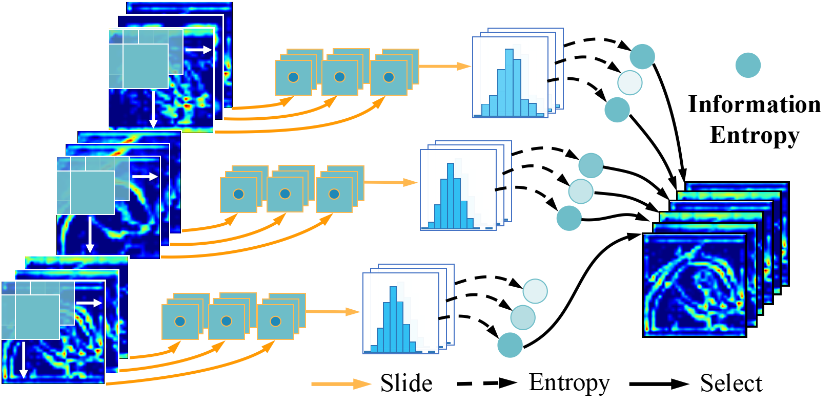
Figure 3: Example of feature selection using 2D information entropy.

2.1 Curvature-based Feature Selection

For a two-dimensional surface embedded in Euclidean space $R^{3}$, two curvatures exist: Gaussian curvature and mean curvature. Compared with the Gaussian curvature, the mean curvature can better reflect the unevenness of the surface. Gong [15] proposed a calculation formula that only requires a simple linear convolution to obtain an approximate mean curvature, as shown below:

$$\bm{C}=\begin{bmatrix}\bm{C_{1}}&\bm{C_{2}}&\bm{C_{3}}\\[2.0pt] \end{bmatrix}\bm{*}\bm{X},$$ (1)

where $\bm{C_{1}}=[\alpha,\beta,\alpha]^{T}$, $\bm{C_{2}}=[\beta,\gamma,\beta]^{T}$, $\bm{C_{3}}=[\alpha,\beta,\alpha]^{T}$, the values of $\alpha$, $\beta$, and $\gamma$ are $-1/16$, $5/16$, $-1$. $\bm{*}$ denotes convolution, $\bm{X}$ represents the input image, and $\bm{C}$ is the mean curvature. Fig. 2 illustrates the process, showing that the curvature image can effectively highlight the edge details in the features.

2.2 Information Entropy-based Feature Selection

As a statistical form of feature, information entropy [1] reflects the spatial and aggregation characteristics of the intensity distribution. It can be formulated as:

$$\ E=-\sum^{255}_{i=0}\sum^{255}_{j=0}P_{i,j}log_{2}\left(P_{i,j}\right)\\ ,\ P_{i,j}=f\left(i_{n},j_{n}\right)/\left(H\times{W}\right),$$ (2)

$i_{n}$ denotes the gray value of the center pixel in the $n^{th}$ $3\times{3}$ sliding window and $j_{n}$ denotes the average gray value of the remaining pixels in that window (teal blue box in Fig. 3). The probability of $\left(i_{n},j_{n}\right)$ occurring in the entire image is denoted by $P_{i,j}$, and $E$ represents the information entropy.

Algorithm 1 Information entropy of features with histogram.

Input:$\bm{F_{x}}\in\mathbb{R^{C\times{H}\times{W}}},bins=256,kernel\_size=3$

Output:$\bm{E}\in\mathbb{R^{C}}$

$z=unfold\left(\bm{F},kernel\_size\right)$ $\triangleright$ Sliding window operation.

$i=flatten\left(z\right)\left[\left({H\times{W}}\right)//2\right]$

$j=\left(sum\left(z\right)-i\right)/{\left(\left({H\times{W}}\right)-1\right)}$

$f_{hist\left(i,j\right)}=histc\left(\left(i,j\right),bins\right)$ $\triangleright$ Compute the histogram of $\left(i,j\right)$.

$ext\_k=kernel\_size//2$

$\bm{P_{hist\left(i,j\right)}}=f_{hist\left(i,j\right)}/\left(\left(H+ext_{k}\right)\times{\left(W+ext_{k}\right)}\right)$

$\bm{E}=sum\left(-\bm{P_{hist\left(i,j\right)}}\times{log_{2}\left(\bm{P_{hist\left(i,j\right)}}\right)}\right)$

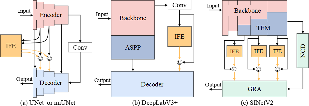
Figure 4: Implementation of IFE in exemplar networks. $\copyright$ is concatenation.

Each pixel on images corresponds to a gray or color value ranging from 0 to 255. However, each element in the feature map represents the activation level of the convolution filter at a particular position in the input image. Given an input feature $\bm{F_{x}}$, as shown in Fig. 3, the tuples $\left(i,j\right)$ obtained by the sliding windows are transformed to a histogram, representing the magnitude of the activation level and distribution within the neighborhood. This involves rearranging the activation levels of the feature map. The histogram converting method $histc$ and information entropy $\bm{E}$ are presented in Algorithm. 1. Note that the probability $\bm{P_{hist\left(i,j\right)}}$ will be used to calculate the information entropy.

2.3 Instructive Feature Enhancement

Although IFE can be applied to various deep neural networks, this study mainly focuses on widely used segmentation networks. Fig. 4 shows the framework of IFE embedded in representative networks, e.g., DeepLabV3+ [9], UNet [28], nnUNet [18], and SINetV2 [14]. The first three are classic segmentation networks. Because the MIS task is similar to the camouflage object detection, such as low contrast and blurred edges, we also consider SINetV2 [14]. According to [27], we implement IFE on the middle layers of UNet [28] and nnUNet [18], on the low-level features of DeepLabV3+ [9], and on the output of the TEM of SINetV2 [14].

While the input images are encoded into the feature space, the different channel features retain textures in various directions and frequencies. Notably, the information contained by the same channel may vary across different images, which can be seen in Fig. 5. For instance, the $15^{th}$ channel of the lung CT feature map contains valuable texture and details, while the same channel in the aortic CT feature map may not provide significant informative content. However, their $2^{nd}$ channel features both focus on the edge details. By preserving the raw features, the channel features that contribute more to the segmentation of the current object can be enhanced by dynamically selecting from the input features. Naturally, it is possible to explicitly increase the sensitivity of the model to the channel information. Specifically, for input image $\mathbf{X}$, the deep feature $\bm{F_{x}}=[f_{1},f_{2},f_{3},\cdots,f_{C}]\in\mathbb{R^{C*H*W}}$ can be obtained by an encoder with the weights $\theta_{x}$: $\bm{F_{x}}=Encoder\left(\mathbf{X},\theta_{x}\right)$, our IFE can be expressed as:

$$\bm{F_{x}^{{}^{\prime}}}=max\{S\left(\bm{F_{x}}\right),r\},$$ (3)

$\bm{F_{x}^{{}^{\prime}}}$ is the selected feature map and $S$ is the quantification method (see Fig. 2 or Fig. 3), and $r$ is the selected proportion. As discussed in [6], enhancing the raw features through pixel-wise addition may introduce unwanted background noise and cause interference. In contrast, the concatenate operation directly joins the features, allowing the network to learn how to fuse them automatically, reducing the interference caused by useless background noises. Therefore, we used the concatenation and employed the concatenated features $\bm{F}=[\bm{F_{x}},\bm{F_{x}^{{}^{\prime}}}]$ as the input to the next stage of the network. Only the initialization channel number of the corresponding network layer needs to be modified.

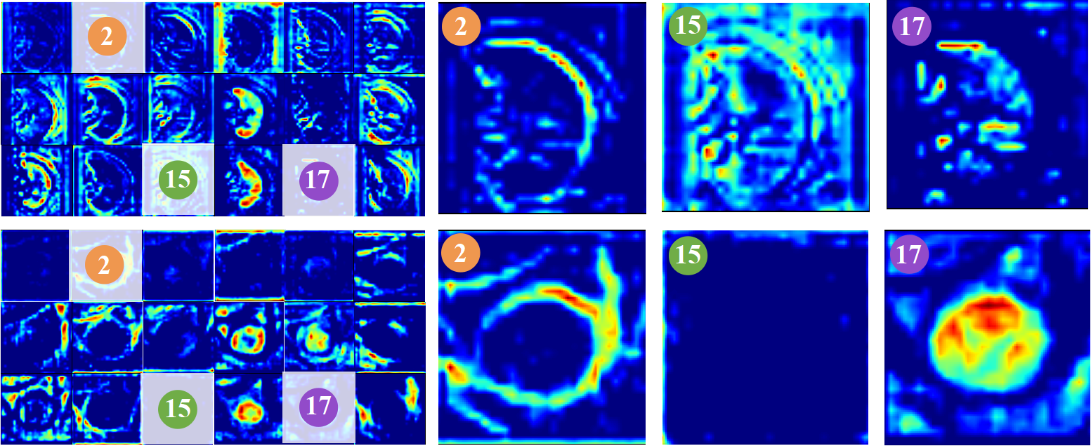
Figure 5: Feature maps visualization of the lung (first row) and aortic (second row) CT images from stage 3 of SINetV2. 2, 15, and 17 are the indexes of channels. The information contained by the same channel may vary across different images.

3 Experimental Results

3.0.1 Cosmos55k.

To construct the large-scale Cosmos55k, 30 publicly available datasets [30, 35, 23, 32, 20, 22, 4, 3, 19, 11, 21, 24, 29] were collected and processed with organizers’ permission. The processing procedures included uniform conversion to PNG format, cropping, and removing mislabeled images. Cosmos55k (Fig. 1) offers 7 imaging modalities, including CT, MRI, X-ray, fundus, etc., covering 26 anatomical structures such as the liver, polyp, melanoma, and vertebra, among others. Images contain just one labeled object, reducing confusion from multiple objects with different structures.

Table 1: Quantitative comparison on IFE. +C, +E means curvature- or information entropy-based IFE. DLV3+ is DeepLabV3+. Bolded means the best group result. $*$ denotes that DSC passed t-test, p < 0.05.

Method	Con(%)$\uparrow$	DSC(%)$\uparrow$	JC(% )$\uparrow$	F1(%)$\uparrow$	HCE$\downarrow$	MAE(%)$\downarrow$	HD$\downarrow$	ASD$\downarrow$	RVD$\downarrow$
UNet	84.410	93.695	88.690	94.534	1.988	1.338	11.464	2.287	7.145
+C	85.666	$94.003^{*}$	89.154	94.528	1.777	1.449	11.213	2.222	6.658
+E	86.664	$\textbf{94.233}^{*}$	89.526	94.466	1.610	1.587	11.229	2.177	6.394
nnUNet	-53.979	92.617	87.267	92.336	2.548	0.257	19.963	3.698	9.003
+C	-30.908	92.686	87.361	92.399	2.521	0.257	19.840	3.615	8.919
+E	-34.750	92.641	87.313	92.367	2.510	0.257	19.770	3.637	8.772
SINetV2	80.824	93.292	88.072	93.768	2.065	1.680	11.570	2.495	7.612
+C	84.883	$\textbf{93.635}^{*}$	88.525	94.152	1.971	1.573	11.122	2.402	7.125
+E	83.655	93.423	88.205	93.978	2.058	1.599	11.418	2.494	7.492
DLV3+	88.566	94.899	90.571	95.219	1.289	1.339	9.113	2.009	5.603
+C	88.943	$95.000^{*}$	90.738	95.239	1.274	1.369	8.885	1.978	5.391
+E	88.886	$\textbf{95.002}^{*}$	90.741	95.103	1.257	1.448	9.108	2.011	5.468

3.0.2 Implementation Details.

Cosmos55k comprises 55,023 images, with 31,548 images used for training, 5,884 for validation, and 17,591 for testing. We conducted experiments using Pytorch for UNet [28], DeeplabV3+ [9], SINetV2 [14], and nnUNet [18]. The experiments were conducted for 100 epochs on an RTX 3090 GPU. The batch sizes for the first three networks were 32, 64, and 64, respectively, and the optimizer used was Adam with an initial learning rate of $10^{-4}$. Every 50 epochs, the learning rate decayed to 1/10 of the former. Considering the large scale span of the images in Cosmos55k, the images were randomly resized to one of seven sizes (224, 256, 288, 320, 352, or 384) before being fed into the network for training. During testing, the images were resized to a fixed size of 224. Notably, the model set the hyperparameters for nnUNet [18] automatically.

Table 2: Ablation studies of UNet about ratio $r$. Bolded means the best result.

Method	Ratio	Con(%)$\uparrow$	DSC(%)$\uparrow$	JC(% )$\uparrow$	F1(%)$\uparrow$	HCE$\downarrow$	MAE(%)$\downarrow$	HD$\downarrow$	ASD$\downarrow$	RVD$\downarrow$
UNet	0,0	84.410	93.695	88.690	94.534	1.988	1.338	11.464	2.287	7.145
	1.0,1.0	84.950	93.787	88.840	94.527	1.921	1.376	11.417	2.271	6.974
+C	0.75,0.75	84.979	93.855	88.952	94.528	1.865	1.405	11.378	2.246	6.875
	0.75,0.50	85.666	94.003	89.154	94.528	1.777	1.449	11.213	2.222	6.658
	0.50,0.50	84.393	93.742	88.767	94.303	1.908	1.497	11.671	2.305	7.115
+E	0.75,0.75	85.392	93.964	89.106	94.290	1.789	1.597	11.461	2.252	6.712
	0.75,0.50	83.803	93.859	88.949	94.420	1.877	1.471	11.351	2.260	6.815
	0.50,0.50	86.664	94.233	89.526	94.466	1.610	1.587	11.229	2.177	6.394

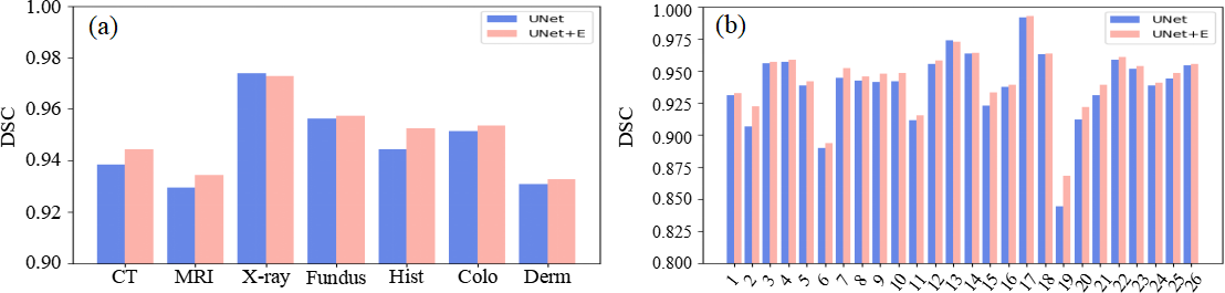
Figure 6: DSC of UNet (blue) and UNet+E (pink) in modalities (a) and anatomic structures (b). Hist, Colo, and Derm are Histopathology, Colonoscopy, and Dermoscopy.

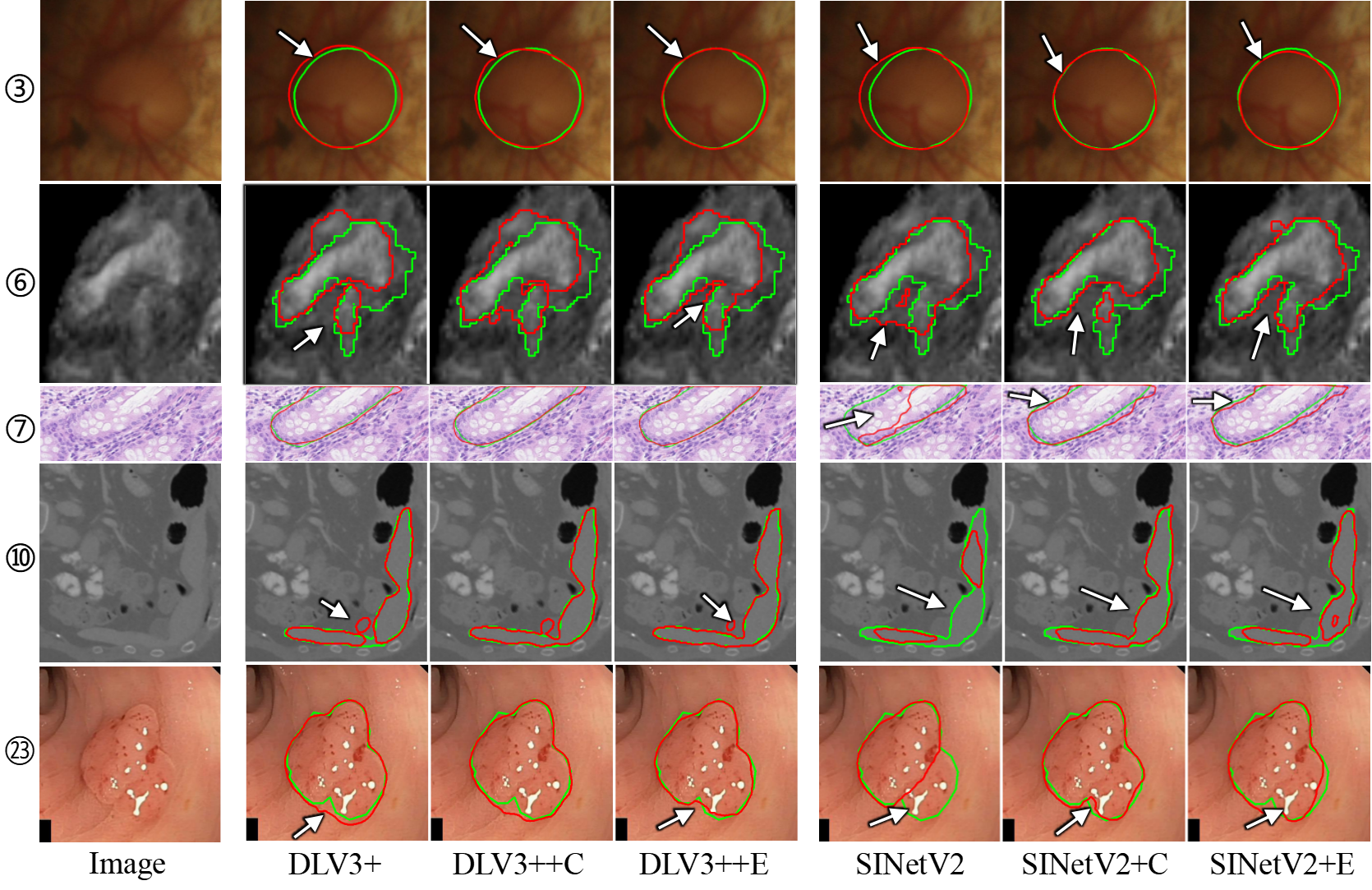
Figure 7: Qualitative comparison of different models equipped with IFE. Red and green denote prediction and ground truth, respectively.

3.0.3 Quantitative and Qualitative Analysis.

To demonstrate the efficacy of IFE, we employ the following metrics: Conformity (Con) [7], Dice Similarity Coefficient (DSC) [5], Jaccard Distance (JC) [12], F1 [2], Human Correction Efforts (HCE) [26], Mean Absolute Error (MAE) [25], Hausdorff Distance (HD) [34], Average Symmetric Surface Distance (ASD) [13], Relative Volume Difference(RVD) [13]. The quantitative results for UNet [28], DeeplabV3+ [9], SINetV2 [14], and nnUNet [18] are presented in Table 1. From the table, it can be concluded that IFE can improve the performance of networks on most segmentation metrics. Besides, Fig. 6 shows that IFE helps models perform better in most modalities and anatomical structures. Fig. 7 presents a qualitative comparison. IFE aids in locating structures in an object that may be difficult to notice and enhances sensitivity to edge gray variations. IFE can substantially improve the segmentation accuracy of the base model in challenging scenes.

3.0.4 Ablation Studies.

Choosing a suitable selection ratio $r$ is crucial when applying IFE to different networks. Different networks’ encoders are not equally capable of extracting features, and the ratio of channel features more favorable to the segmentation result varies. To analyze the effect of $r$, we conducted experiments using UNet [28]. As shown in Table 2, either too large or too small $r$ will lead to a decline in the model performance.

4 Conclusion

In order to benchmark the general DMIS, we build a large-scale dataset called Cosmos55k. To balance universality and accuracy, we proposed an approach (IFE) that can select instructive feature channels to further improve the segmentation over strong baselines against challenging tasks. Experiments showed that IFE can improve the performance of classic models with slight modifications in the network. It is simple, universal, and effective. Future research will focus on extending this approach to 3D tasks.

4.0.1 Acknowledgements.

The authors of this paper sincerely appreciate all the challenge organizers and owners for providing the public MIS datasets including AbdomenCT-1K, ACDC, AMOS 2022, BraTS20, CHAOS, CRAG, crossMoDA, EndoTect 2020, ETIS-Larib Polyp DB, iChallenge-AMD, iChallenge-PALM, IDRiD 2018, ISIC 2018, I2CVB, KiPA22, KiTS19$\&$KiTS21, Kvasir-SEG, LUNA16, Multi-Atlas Labeling Beyond the Cranial Vault (Abdomen), Montgomery County CXR Set, M&Ms, MSD, NCI-ISBI 2013, PROMISE12, QUBIQ 2021, SIIM-ACR, SLIVER07, VerSe19$\&$VerSe20, Warwick-QU, and WORD.

This work was supported by the grant from National Natural Science Foundation of China (Nos. 62171290, 62101343), Shenzhen-Hong Kong Joint Research Program (No. SGDX20201103095613036), and Shenzhen Science and Technology Innovations Committee (No. 20200812143441001).

References

- [1] Abdel-Khalek, S., Ishak, A.B., Omer, O.A., Obada, A.S.: A two-dimensional image segmentation method based on genetic algorithm and entropy. Optik 131, 414–422 (2017)
- [2] Achanta, R., Hemami, S., Estrada, F., Susstrunk, S.: Frequency-tuned salient region detection. In: IEEE CVPR (2009)
- [3] Bakas, S., Reyes, M., Jakab, A., Bauer, S., Rempfler, M., Crimi, A., Shinohara, R.T., Berger, C., Ha, S.M., Rozycki, M., et al.: Identifying the best machine learning algorithms for brain tumor segmentation, progression assessment, and overall survival prediction in the brats challenge. arXiv preprint arXiv:1811.02629 (2018)
- [4] Bernard, O., Lalande, A., Zotti, C., Cervenansky, F., Yang, X., Heng, P.A., Cetin, I., Lekadir, K., Camara, O., Ballester, M.A.G., et al.: Deep learning techniques for automatic mri cardiac multi-structures segmentation and diagnosis: is the problem solved? IEEE TMI 37(11), 2514–2525 (2018)
- [5] Bilic, P., Christ, P., Li, H.B., Vorontsov, E., Ben-Cohen, A., Kaissis, G., Szeskin, A., Jacobs, C., Mamani, G.E.H., Chartrand, G., et al.: The liver tumor segmentation benchmark (lits). MIA 84, 102680 (2023)
- [6] Cao, G., Xie, X., Yang, W., Liao, Q., Shi, G., Wu, J.: Feature-fused ssd: Fast detection for small objects. In: SPIE ICGIP. vol. 10615 (2018)
- [7] Chang, H.H., Zhuang, A.H., Valentino, D.J., Chu, W.C.: Performance measure characterization for evaluating neuroimage segmentation algorithms. Neuroimage 47(1), 122–135 (2009)
- [8] Chen, L.C., Papandreou, G., Kokkinos, I., Murphy, K., Yuille, A.L.: Deeplab: Semantic image segmentation with deep convolutional nets, atrous convolution, and fully connected crfs. IEEE TPAMI 40(4), 834–848 (2017)
- [9] Chen, L.C., Zhu, Y., Papandreou, G., Schroff, F., Adam, H.: Encoder-decoder with atrous separable convolution for semantic image segmentation. In: ECCV (2018)
- [10] Chollet, F.: Xception: Deep learning with depthwise separable convolutions. In: IEEE CVPR (2017)
- [11] Codella, N.C., Gutman, D., Celebi, M.E., Helba, B., Marchetti, M.A., Dusza, S.W., Kalloo, A., Liopyris, K., Mishra, N., Kittler, H., et al.: Skin lesion analysis toward melanoma detection: A challenge at the 2017 international symposium on biomedical imaging (isbi), hosted by the international skin imaging collaboration (isic). In: ISBI (2018)
- [12] Crum, W.R., Camara, O., Hill, D.L.: Generalized overlap measures for evaluation and validation in medical image analysis. IEEE TMI 25(11), 1451–1461 (2006)
- [13] Dubuisson, M.P., Jain, A.K.: A modified hausdorff distance for object matching. In: IEEE ICPR (1994)
- [14] Fan, D.P., Ji, G.P., Cheng, M.M., Shao, L.: Concealed object detection. IEEE TPAMI 44(10), 6024–6042 (2021)
- [15] Gong, Y., Sbalzarini, I.F.: Curvature filters efficiently reduce certain variational energies. IEEE TIP 26(4), 1786–1798 (2017)
- [16] Hou, Q., Zhou, D., Feng, J.: Coordinate attention for efficient mobile network design. In: IEEE CVPR (2021)
- [17] Howard, A., Sandler, M., Chu, G., Chen, L.C., Chen, B., Tan, M., Wang, W., Zhu, Y., Pang, R., Vasudevan, V., et al.: Searching for mobilenetv3. In: IEEE ICCV (2019)
- [18] Isensee, F., Jaeger, P.F., Kohl, S.A., Petersen, J., Maier-Hein, K.H.: nnu-net: a self-configuring method for deep learning-based biomedical image segmentation. Nature methods 18(2), 203–211 (2021)
- [19] Jha, D., Smedsrud, P.H., Riegler, M.A., Halvorsen, P., de Lange, T., Johansen, D., Johansen, H.D.: Kvasir-seg: A segmented polyp dataset. In: MMM (2020)
- [20] Ji, W., Yu, S., Wu, J., Ma, K., Bian, C., Bi, Q., Li, J., Liu, H., Cheng, L., Zheng, Y.: Learning calibrated medical image segmentation via multi-rater agreement modeling. In: IEEE CVPR (2021)
- [21] Ji, Y., Bai, H., Yang, J., Ge, C., Zhu, Y., Zhang, R., Li, Z., Zhang, L., Ma, W., Wan, X., et al.: Amos: A large-scale abdominal multi-organ benchmark for versatile medical image segmentation. arXiv preprint arXiv:2206.08023 (2022)
- [22] Kavur, A.E., Gezer, N.S., Barış, M., Aslan, S., Conze, P.H., Groza, V., Pham, D.D., Chatterjee, S., Ernst, P., Özkan, S., et al.: Chaos challenge-combined (ct-mr) healthy abdominal organ segmentation. MIA 69, 101950 (2021)
- [23] Litjens, G., Toth, R., Van De Ven, W., Hoeks, C., Kerkstra, S., van Ginneken, B., Vincent, G., Guillard, G., Birbeck, N., Zhang, J., et al.: Evaluation of prostate segmentation algorithms for mri: the promise12 challenge. MIA 18(2), 359–373 (2014)
- [24] Luo, X., Liao, W., Xiao, J., Chen, J., Song, T., Zhang, X., Li, K., Metaxas, D.N., Wang, G., Zhang, S.: Word: A large scale dataset, benchmark and clinical applicable study for abdominal organ segmentation from ct image. MIA 82, 102642 (2022)
- [25] Perazzi, F., Krähenbühl, P., Pritch, Y., Hornung, A.: Saliency filters: Contrast based filtering for salient region detection. In: IEEE CVPR (2012)
- [26] Qin, X., Dai, H., Hu, X., Fan, D.P., Shao, L., Gool, L.V.: Highly accurate dichotomous image segmentation. In: ECCV (2022)
- [27] Raghu, M., Unterthiner, T., Kornblith, S., Zhang, C., Dosovitskiy, A.: Do vision transformers see like convolutional neural networks? Advances in Neural Information Processing Systems 34, 12116–12128 (2021)
- [28] Ronneberger, O., Fischer, P., Brox, T.: U-net: Convolutional networks for biomedical image segmentation. In: MICCAI (2015)
- [29] Sekuboyina, A., Husseini, M.E., Bayat, A., Löffler, M., Liebl, H., Li, H., Tetteh, G., Kukačka, J., Payer, C., Štern, D., et al.: Verse: A vertebrae labelling and segmentation benchmark for multi-detector ct images. MIA 73, 102166 (2021)
- [30] Simpson, A.L., Antonelli, M., Bakas, S., Bilello, M., Farahani, K., Van Ginneken, B., Kopp-Schneider, A., Landman, B.A., Litjens, G., Menze, B., et al.: A large annotated medical image dataset for the development and evaluation of segmentation algorithms. arXiv preprint arXiv:1902.09063 (2019)
- [31] Szegedy, C., Ioffe, S., Vanhoucke, V., Alemi, A.: Inception-v4, inception-resnet and the impact of residual connections on learning. In: AAAI (2017)
- [32] Zhao, Z., Chen, H., Wang, L.: A coarse-to-fine framework for the 2021 kidney and kidney tumor segmentation challenge. In: MICCAI (2022)
- [33] Zhong, Z., Lin, Z.Q., Bidart, R., Hu, X., Daya, I.B., Li, Z., Zheng, W.S., Li, J., Wong, A.: Squeeze-and-attention networks for semantic segmentation. In: IEEE CVPR (2020)
- [34] Zhou, D., Fang, J., Song, X., Guan, C., Yin, J., Dai, Y., Yang, R.: Iou loss for 2d/3d object detection. In: IEEE 3DV (2019)
- [35] Zhou, Y., Li, Z., Bai, S., Wang, C., Chen, X., Han, M., Fishman, E., Yuille, A.L.: Prior-aware neural network for partially-supervised multi-organ segmentation. In: IEEE ICCV (2019)
- [36] Zhou, Z., Siddiquee, M.M.R., Tajbakhsh, N., Liang, J.: Unet++: Redesigning skip connections to exploit multiscale features in image segmentation. IEEE TMI 39(6), 1856–1867 (2019)