Efficient Anomaly Detection with Budget Annotation Using Semi-Supervised Residual Transformer

Abstract

Anomaly Detection (AD) is challenging as usually only the normal samples are seen during training and the detector needs to discover anomalies on-the-fly. The recently proposed deep-learning-based approaches could somehow alleviate the problem but there is still a long way to go in obtaining an industrial-class anomaly detector for real-world applications. On the other hand, in some particular AD tasks, a few anomalous samples are labeled manually for achieving higher accuracy. However, this performance gain is at the cost of considerable annotation efforts, which can be intractable in many practical scenarios.

In this work, the above two problems are addressed in a unified framework. Firstly, inspired by the success of the patch-matching-based AD algorithms, we train a sliding vision transformer over the residuals generated by a novel position-constrained patch-matching. Secondly, the conventional pixel-wise segmentation problem is cast into a block-wise classification problem. Thus the sliding transformer can attain even higher accuracy with much less annotation labor. Thirdly, to further reduce the labeling cost, we propose to label the anomalous regions using only bounding boxes. The unlabeled regions caused by the weak labels are effectively exploited using a highly-customized semi-supervised learning scheme equipped with two novel data augmentation methods. The proposed method, termed “Semi-supervised RESidual Transformer” or “SemiREST” in short, outperforms all the state-of-the-art approaches using all the evaluation metrics in both the unsupervised and supervised scenarios. On the popular MVTec-AD dataset, our SemiREST algorithm obtains the Average Precision (AP) of $81.2\%$ (vs. previous best result of AP $75.8\%$) in the unsupervised condition and $84.4\%$ AP (vs. previous best result of AP $78.6\%$) for supervised anomaly detection. Surprisingly, with the bounding-box-based semi-supervisions, SemiREST still outperforms the SOTA methods with full supervision ($83.8\%$ AP vs. previous SOTA AP $78.6\%$) on MVTec-AD. Similar precision advantages are also observed on the other two well-known AD datasets, i.e., BTAD, and KSDD2. Overall, the proposed SemiREST generates new records of AD performances while at a remarkably low annotation cost. It is not only cheaper in annotation but also performs better than most recent methods. The code of this work is available at: https://github.com/BeJane/Semi_REST

1 Introduction

Product quality control is crucial in many manufacturing processes. Manual inspection is expensive and unreliable considering the limited time budget for inspection on a running assembly line. As a result, automatic defect inspection is compulsory in modern manufacturing industries Niu et al. (2021); Ni et al. (2021); Tao et al. (2022); Cao et al. (2023b). Given training samples with sufficient supervision, it is straightforward to perform defect detection using off-the-shelf detection or segmentation algorithms Cheng et al. (2018); Wang et al. (2022a, c, b). Unfortunately, in most practical cases, one can only obtain much fewer “anomaly” samples than the normal ones and the anomaly pattern varies dramatically over different samples. As a result, the defect detection task is often cast into an Anomaly Detection (AD) problem Bergmann et al. (2019); Mishra et al. (2021), with only normal instances supplied for training.

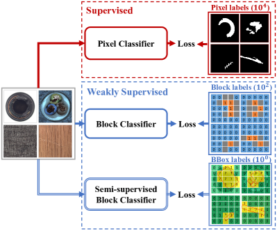
Figure 1: The comparison of our framework with the conventional paradigm. The annotation strength can be divided into three levels, as shown in the three rows on the right-hand side of the figure. Top (conventional): pixel-wise segmentation for anomaly detection; middle (proposed): solving the AD problem as block-wise binary classifications with negative samples, positive samples, and ignored samples are shown in blue, orange, and gray respectively; bottom (proposed): a more aggressive semi-supervised manner with only bonding boxes labeled for the anomaly regions. The numbers in the parenthesis denote the decreasing order of magnitudes (from $10^{4}$ to $10^{0}$) of the annotation numbers under the three supervision conditions. Better view in color.

During the past few years, a great amount of effort has been invested in developing better AD algorithms. First of all, inspired by the pioneering works Scholkopf et al. (2000); Schölkopf et al. (2001), a large part of AD literature focus on modeling normal images or patches as a single class while the abnormal ones are detected as outliers Ruff et al. (2018); Yi and Yoon (2020); Liznerski et al. (2021); Massoli et al. (2021); Defard et al. (2021); Zhang et al. (2022); Chen et al. (2022). Normalizing Flow Dinh et al. (2014, 2016); Kingma and Dhariwal (2018) based AD algorithms propose to further map the normal class to fit a Gaussian distribution in the feature spaceRudolph et al. (2021); Yu et al. (2021); Tailanian et al. (2022); Lei et al. (2023). Secondly, by observing that most normal samples can be effectively reconstructed by other normal ones, a number of researchers have tried to conduct the reconstruction in various spaces for the test images or image patches and estimate the anomaly scores based on the reconstruction residuals Zong et al. (2018); Dehaene and Eline (2020); Shi et al. (2021); Hou et al. (2021); Wu et al. (2021). In addition to the reconstruction, some more sophisticated anomaly detectors Li et al. (2021); Zavrtanik et al. (2021); Yang et al. (2023) also learn discriminative models with “pseudo anomalies” for higher accuracy. At the other end of the spectrum, however, the seminar work Roth et al. (2022) shows that a well-designed nearest-neighbor matching process can already achieve sufficiently good detection accuracies. Thirdly, to obtain distinct responses to anomaly inputs, distillation-based approaches Salehi et al. (2021); Deng and Li (2022); Bergmann et al. (2022); Zhang et al. (2023b) distill a “teacher network” (which is pre-trained on a large but “neutral” dataset) into a “student network” only based on normal samples. Then the anomaly score can be calculated according to the response differences between the two networks. Last but not least, inspired by the prior observations that the position information of image patches may benefit the AD processes Gudovskiy et al. (2022); Bae et al. (2022), researchers further propose to geometrically align the test images with the reference ones and perform local comparisons between the aligned images and their prototypes Huang et al. (2022); Liu et al. (2023a).

Despite the mainstream “unsupervised” fashion, in Ding et al. (2022); Zhang et al. (2023a); Yao et al. (2023), anomaly detectors are trained in a “few-shot” manner and unsurprisingly higher performances are achieved, compared with their “zero-shot” counterparts. In addition, the traditional surface defect detection tasks Tabernik et al. (2020); Huang et al. (2020); Zhang et al. (2021b); Božič et al. (2021) are mostly solved in a fully-supervised version. Considering that in practice, the detection algorithm needs to “warm-up” for a certain duration along with the running assemble-line, the abnormal samples are not difficult to obtain in this scenario. And thus this “supervised” setting is actually valid.

In this paper, we claim that compared with the lack of the training anomalies, a more realistic problem to address is the limited time budget for labeling the newly-obtained anomalous images. Accordingly, we propose a novel AD algorithm that simultaneously enjoys high detection robustness and low annotation cost. The high-level concept of the proposed algorithm is illustrated in Figure 1. Compared with the conventional pixel-wise supervision, the proposed method can utilize weak labels, i.e., the block labels or bounding-box labels (as shown in the bottom part of Figure 1) to get even higher AD performances.

In specific, we consider the AD task as a block-wise classification problem (as shown in the right-middle part of Figure 1) and thus one only needs to label hundreds of anomaly blocks instead of thousands of anomaly pixels on a defective image. The patch-matching residual is generated for each block constrained by the block’s position-code. And then the blocks are classified by a sliding Swin Transformer (Liu et al., 2021) that receives the patch-matching residuals as its tokens. The final anomaly score of a block is obtained via a bagging process over all the Swin Transformers whose input involves this block. Thanks to the novel features and the bagging strategy, the proposed algorithm performs better than those with pixel-level supervision. More aggressively, we propose to further reduce the annotation cost by labeling the anomaly regions with only bounding boxes. As can be seen in the right-bottom part of Figure 1, the boxes cover all the anomaly regions of the image so the outside blocks (shown in green) can be directly used as negative samples. On the other hand, the identities of the inside blocks (shown in yellow) are not given and seem useless in the conventional learning paradigm. In this work, nonetheless, the unlabeled blocks are utilized effectively via a modified Mix-Match (Berthelot et al., 2019b) algorithm that is smartly customized for the transformer-based anomaly detector. The productive utilization of the unlabeled information reduces the performance drop from full supervision.

We term the proposed AD algorithm as “Semi-supervised RESidual Transformer” or “SemiREST” in short. Our experiments in this paper verify the superiority of the proposed method: SemiREST outperforms all the state-of-the-art AD algorithms on the three well-known datasets (MVTec-AD (Bergmann et al., 2019), BTAD (Mishra et al., 2021) and KSDD2 (Božič et al., 2021)) in both the mainstream “unsupervised” setting and the “few-shot” setting. In addition, with only bounding-box annotations, the SemiREST also beats all the SOTA methods with fully-supervised pixel labels with all the employed evaluation metrics. In summary, our main contribution is three fold, as listed below.

• Cheaper in terms of annotation: From a realistic perspective, we suggest that, compared with the “one-class” compatibility, a more desirable property for AD algorithms is the high efficiency of using annotation information. Accordingly, this work proposes two types of low-cost annotations: the block-wise labels and the bounding box labels. To the best of our knowledge, it is the first time that the block-wise label is used for anomaly detection and the usage of the bounding-box label in the context of semi-supervised AD learning is also creative.

• Better: We design the SemiREST algorithm based on a modified Swin-Transformer Liu et al. (2021) and the patch-matching residuals generated with position-code constraints. The proposed algorithm consistently surpasses the SOTA methods by large margins, on the three most acknowledged datasets and in all the supervision conditions.

• Cheaper & Better: Given the cheap bounding-box labels, SemiREST could effectively utilize the unlabeled features thanks to the highly-customized MixMatch (Berthelot et al., 2019b) algorithm proposed in this work. Merely with these lightweight annotations, SemiREST still outperforms ALL the comparing SOTA methods fed with fully annotated pixel-wise labels.

2 Related work

2.1 Anomaly Detection via Patch Feature Matching

A straightforward way for realizing AD is to compare the test patch with the normal patches. The test patches similar to the normal ones are considered to be unlikely to be anomalies while those with low similarities are assigned with high anomaly scores. PatchCore algorithm (Roth et al., 2022) proposes the coreset-subsampling algorithm to build a “memory bank” of patch features, which are obtained via smoothing the neutral deep features pre-learned on ImageNet (Deng et al., 2009; Russakovsky et al., 2015). The anomaly score is then calculated based on the Euclidean distance between the test patch feature and its nearest neighbor in the “memory bank”. Despite the simplicity, PatchCore performs dramatically well on the MVTec-AD dataset (Bergmann et al., 2019).

The good performance of PatchCore encourages researchers to develop better variants based on it. The PAFM algorithm (Kim et al., 2022) applies patch-wise adaptive coreset sampling to improve the speed. (Bae et al., 2022) introduces the position and neighborhood information to refine the patch-feature comparison. Graphcore (Xie et al., 2023) utilizes graph representation to customize PatchCore for the few-shot setting. (Saiku et al., 2022) modifies PatchCore by compressing the memory bank via k-means clustering. (Zhu et al., 2022) combines PatchCore (Roth et al., 2022) and Defect GAN (Zhang et al., 2021a) for higher AD performances.

Those variants, though achieving slightly better performances, all fail in noticing the potential value of the intermediate information generated by the patch-matching. In this work, we use the matching residuals as the input tokens of our transformer model. The individual and the mutual information of the residuals are effectively exploited and new SOTA performances are then obtained.

2.2 Swin Transformer for Anomaly Detection

As a variation of Vision Transformer (ViT) (Dosovitskiy et al., 2021), Swin Transformer (Liu et al., 2021, 2022) proposed a hierarchical Transformer with a shifted windowing scheme, which not only introduces several visual priors into Transformer but also reduces computation costs. Swin Transformer its variants illustrate remarkable performances in various computer vision tasks, such as semantic segmentation (Huang et al., 2021; Hatamizadeh et al., 2022; Cao et al., 2023a), instance segmentation (Dong et al., 2021; Li et al., 2022) and object detection (Xu et al., 2021; Dai et al., 2021; Liang et al., 2022).

In the literature on anomaly detection, some recently proposed methods also employ Swin-Transformer as the backbone network. (Üzen et al., 2022) develops a hybrid structure decoder that combines convolution layers and the Swin Transformer. (Gao et al., 2022) improves the original shifted windowing scheme of the Swin-Transformer for surface defect detection. Despite the success of Swin Transformer models in other domains, the Swin-Transformer-based AD algorithms could hardly outperform the SOTA methods on most acknowledged datasets such as (Bergmann et al., 2019), (Mishra et al., 2021) and (Božič et al., 2021).

In this paper, we successfully tame the Swin Transformer for the small training sets of AD problems by introducing a series of novel modifications.

2.3 MixMatch and Weak Labels based on Bounding Boxes

Semi-supervised Learning (SSL) is always attractive since it can save massive labeling labor. Many efforts have been devoted to utilizing the information from the unlabeled data (Zhu and Goldberg, 2009; Berthelot et al., 2019b, a; Sohn et al., 2020; Wang et al., 2023), mainly focusing on the generation of high-quality pseudo labels. Inspired by the seminar work (Zhang et al., 2018; Yun et al., 2019) for data augmentation, MixMatch proposes a single-loss SSL method that relies on a smart fusion process between labeled and unlabeled samples. In this way, MixMatch enjoys high accuracy and a relatively simple training scheme.

On the other hand, in the literature on semantic segmentation, bounding boxes are usually used as weak supervision to save labeling costs. (Hsu et al., 2019) exploits the tightness prior to the bounding boxes to generate the positive and negative bags for multiple instance learning (MIL), which is integrated into a fully supervised instance segmentation network. (Kervadec et al., 2020) integrates the tightness prior and a global background emptiness constraint derived from bounding box annotations into a weak semantic segmentation of medical images. (Lee et al., 2021) propose a bounding box attribution map (BBAM) to produce pseudo ground-truth for weakly supervised semantic and instance segmentation.

In this work, within the block-wise classification framework, MixMatch is smartly employed to exploit the information of unlabeled blocks which are brought by the weak supervision of bounding boxes. This combination between MixMatch and the bounding box labels is remarkably effective according to the experiment results and also novel in the literature, to our best knowledge.

3 The proposed method

3.1 Swin Transformer Bagging with Position-constrained Residuals

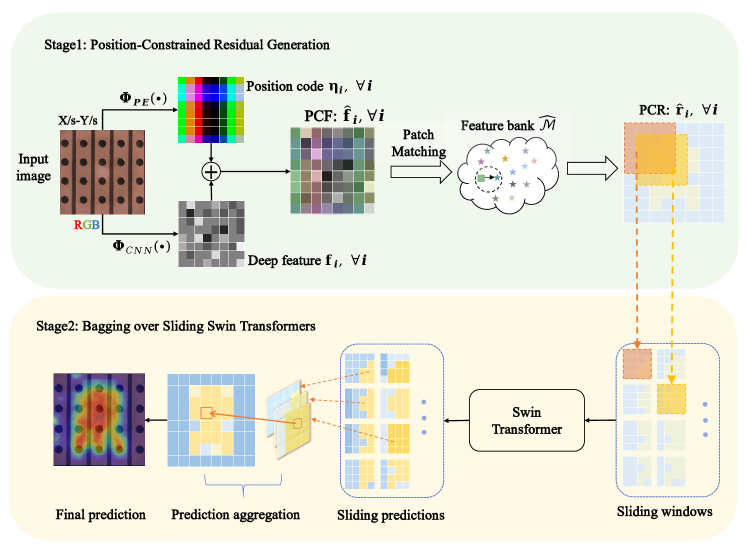
Figure 2: The overview of the inference process of SemiREST. Note that all the tensors with a number of channels are all shown as matrix for the reason of simplicity. Better view in color.

The overall inference process of our SemiREST algorithm is illustrated in Figure 2. As it can be seen, there are two stages in the whole process, i.e., the generation of position-constrained residual features (the green box) and the bagging process over sliding Swin Transformers (the yellow box).

3.1.1 Position constrained residual features

As mentioned in Section 2.1, we try to exploit the potential usage of the intermediate product of the patch-matching process in PatchCore (Roth et al., 2022). In this work, the feature-matching difference vector, rather than the euclidean distance between matched features, is used as the network input. Similar usage of the matching differences can also be find in some recently proposed methods (Ding et al., 2022; Zhang et al., 2023a), but they focus on the residual tensors between two holistic feature maps rather than the residual vectors between two feature vectors. Besides, some new evidences show that positional information of the comparing patches could improve the AD performance (Bae et al., 2022; Gudovskiy et al., 2022) mainly because of the rough alignment of the test images captured in the industrial environment. Accordingly, we introduce the “positional embedding” concept from the literature of Transformers (Dosovitskiy et al., 2021; Liu et al., 2021) to the PatchCore algorithm: the original patch features are aggregated with their positional features encoded in the Transformer way. In this way, the whole patch feature matching process is constrained by the positional information and the ablation study in Section 4.8 verifies the merit of this constraint.

Mathematically, for a input image $\mathrm{I}\in\mathbb{R}^{h_{\mathrm{I}}\times w_{\mathrm{I}}\times 3}$, one can extract deep features as

$$[\mathbf{f}_{1},\mathbf{f}_{2},\cdots,\mathbf{f}_{M}]\leftarrow\mathrm{Flatten}\leftarrow\mathfrak{F}=\Psi_{\mathrm{CNN}}(\mathrm{I})$$ (1)

where $\Psi_{\mathrm{CNN}}(\cdot)$ represents a deep network, which is pre-trained on a large but neutral dataset (ImageNet (Russakovsky et al., 2015) for example); $\mathfrak{F}\in\mathbb{R}^{h_{f}\times w_{f}\times d_{f}}$ denotes the generated deep feature tensor with $M$ feature vectors ($M=h_{f}\cdot w_{f}$); $\mathbf{f}_{i}\in\mathbb{R}^{d_{f}},i=1,2,\cdots,M$ stands for the $i$-th deep feature vector extracted from the tensor $\mathfrak{F}$ on the row-column position $\mathbf{p}_{i}=[r^{f}_{i},c^{f}_{i}]$ and $c^{f}_{i}\in[0,w_{f}),r^{f}_{i}\in[0,h_{f})$.

For a deep feature $\mathbf{f}_{i}$, we modify it and generate its “Position-Constrained Feature” (PCF) as

$$\hat{\mathbf{f}}_{i}=\mathbf{f}_{i}+\lambda_{\mathrm{PE}}\boldsymbol{\eta}_{i}=\mathbf{f}_{i}+\lambda_{\mathrm{PE}}\Phi_{\mathrm{PE}}(\mathbf{p}_{i})$$ (2)

where $\boldsymbol{\eta}=\Phi_{\mathrm{PE}}(\mathbf{p}_{i})\in\mathbb{R}^{d_{f}}$ is termed “position code” (PE) in this paper, with its weight paramerter $\lambda_{\mathrm{PE}}$ and the function $\Phi_{\mathrm{PE}}(\cdot)$ denotes the positional embedding process that calculates the $k$-th element of $\boldsymbol{\eta}$ as

$$\eta^{(k)}_{i}=\begin{cases}\mathrm{sin}(\dfrac{c^{f}_{i}/\rho}{10000^{8k/d_{f}}})&k\in[0,\dfrac{d_{f}}{4})\\ \mathrm{cos}(\dfrac{c^{f}_{i}/\rho}{10000^{8(k-d_{f}/4)/d_{f}}})&k\in[\dfrac{d_{f}}{4},\dfrac{d_{f}}{2})\\ \mathrm{sin}(\dfrac{r^{f}_{i}/\rho}{10000^{8(k-d_{f}/2)/d_{f}}})&k\in[\dfrac{d_{f}}{2},\dfrac{3d_{f}}{4})\\ \mathrm{cos}(\dfrac{r^{f}_{i}/\rho}{10000^{8(k-3d_{f}/4)/d_{f}}})&k\in[\dfrac{3d_{f}}{4},d_{f})\end{cases}$$ (3)

where $\rho$ is the token patch size which will be explained in Section 3.1.2.

Note that Equation 3 mainly follows the positional embedding method used in (He et al., 2022). Better position code may be obtained via a careful design of $\Phi_{\mathrm{PE}}(\cdot)$, but that is out of the scope of this work.

One then can build the memory bank following the method proposed in (Roth et al., 2022) as

$$\hat{\mathcal{M}}=\Psi(\mathcal{F}_{\mathrm{trn}})=\{\hat{\mathbf{m}}_{t}\in\mathbb{R}^{d_{f}}\mid t=1,2,\cdots,T\}$$ (4)

where $\hat{\mathcal{M}}$ is the memory bank containing $T$ PCFs ($\hat{\mathbf{m}}_{t},\forall t$), $\Psi(\cdot)$ represents the sophisticated sampling scheme of PatchCore (Roth et al., 2022), $\hat{\mathcal{F}}_{\mathrm{trn}}=\{\hat{\mathbf{f}}_{i}\in\mathbb{R}^{d_{f}}\mid i=1,2,\cdots,N\}$ denotes the original feature set consisting $N$ PCFs, which are extracted from all the normal images for training.

Finally, given a test PCF $\hat{\mathbf{f}}_{i}$, the corresponding “Position constrained Residual” (PCR) can be calculated in the PatchCore manner (Roth et al., 2022) as

$$\hat{\mathbf{r}}_{i}=\mathcal{S}\left(\hat{\mathbf{f}}_{i}-\mathop{\arg\min}\limits_{\forall\hat{\mathbf{m}}_{t}\in\hat{\mathcal{M}}}\|\hat{\mathbf{f}}_{i}-\hat{\mathbf{m}}_{t}\|_{l_{2}}\right)\in\mathbb{R}^{d_{f}},$$ (5)

with the element-wise square function $\mathcal{S}(\cdot)$ defined as

$$\mathcal{S}\left([x_{1},x_{2},\cdots,x_{d_{f}}]^{\mathrm{T}}\right)=[x^{2}_{1},x^{2}_{2},\cdots,x^{2}_{d_{f}}]^{\mathrm{T}}.$$ (6)

Compared with the absolute values of the tensor difference employed in Zhang et al. (2023a), the yielded residual vector ($\hat{\mathbf{r}}_{i}$) of Equation 6 is more sparse and this “feature-selection” property empirically benefits the following training process, as it is shown in Section 4.8.

According to Equations 1 and 5, we can generate $M$ PCRs from a test image $\mathrm{I}$ as shown in Figure 2. The $M$ PCRs are then reorganized to form the PCR tensor $\hat{\mathfrak{R}}\in\mathbb{R}^{h_{f}\times w_{f}\times d_{f}}$.

3.1.2 Bagging over sliding Swin Transformers

The Swin Transformer is adopted as the backbone of our deep learning model with the PCRs as its input features, rather than normal images. Follow the conventional ViT way (Dosovitskiy et al., 2021; Liu et al., 2021, 2022), the collection of PCRs $\hat{\mathfrak{R}}$ is firstly partitioned into several “feature patches” over the “Row-Column” plane. Given the pre-defined patch size $\rho$, the flattened transformer tokens are stored in the token tensor

$$\mathfrak{T}\in\mathbb{R}^{h_{t}\times w_{t}\times d_{t}},$$ (7)

with the row number $h_{t}={h_{f}}/{\rho}$, column number $w_{t}={w_{f}}/{\rho}$ and the channel dimension $d_{t}=d_{f}\rho^{2}$. Note that here every token vector $\mathrm{t}\in\mathbb{R}^{d_{t}}$ geometrically corresponds to a $(h_{\mathrm{I}}\rho/{h_{t}})\times(w_{\mathrm{I}}\rho/w_{t})$ image-pixel block on the image input of $\Psi_{\mathrm{CNN}}$.

As it is illustrated in Figure 2, a number of “sub-tensors” are extracted from $\mathfrak{T}$ in a sliding-window fashion. Let us define the square windows sliding on the Row-Column plane as:

$$\mathbf{w}=[r^{t},c^{t},\mu]^{\mathrm{T}}$$

where $[r^{t},c^{t}]$ stands for the coordinate of the window’s top-left corner; $\mu$ is the size of the square window; $c^{t}\in[0,w_{t}-\mu)$ and $r^{t}\in[0,h_{t}-\mu)$. A sub-tensor is sliced from $\mathfrak{T}$ according to $\mathbf{w}$ as:

$$\mathfrak{T}_{\mathbf{w}}=\mathfrak{T}[r^{t}:r^{t}+\mu-1,c^{t}:c^{t}+\mu-1,:]\in\mathbb{R}^{\mu\times\mu\times d_{t}}.$$ (8)

The sub-tensor is then fed into the Swin Transformer model to generate the prediction map as

$$\Psi_{\mathrm{Swin}}(\mathfrak{T}_{\mathbf{w}})=\Theta_{\mathbf{w}}\in\mathbb{R}^{\mu\times\mu}.$$ (9)

Note that the output of $\Psi_{\mathrm{Swin}}(\cdot)$ for each token is actually a $2$-D vector, we directly copy the confidences corresponding to the anomaly class to $\Theta_{\mathbf{w}}$.

In specific, given a pre-defined sampling step $s$ and a fixed size $\mu$, one can generates $Q$ square sliding windows $\{\mathbf{w}_{1},\mathbf{w}_{2},\cdots,\mathbf{w}_{Q}\}$ and the corresponding prediction maps $\{\Theta_{\mathbf{w}_{1}},\Theta_{\mathbf{w}_{2}},\cdots,\Theta_{\mathbf{w}_{Q}}\}$. Now each element of the final prediction map $\Theta\in\mathbb{R}^{h_{t}\times w_{t}}$ for the holistic tensor $\mathfrak{T}$ can be calculated as

$$\Theta(r,c)=\frac{1}{|\mathcal{N}_{r,c}|}\sum_{i\in\mathcal{N}_{r,c}}\Theta_{\mathbf{w}_{i}}(r-r^{t}_{i},c-c^{t}_{i})$$ (10)

where $r\in[0,h_{t})$ and $c\in[0,w_{t})$ are the row and column indexes of the map element; $\mathcal{N}_{r,c}$ stands for the set of sliding windows overlapping with location $(r,c)$; $|\cdot|$ represents the set cardinality; the subtractions $r-r^{t}_{i}$ and $c-c^{t}_{i}$ are the coordinate translation operations.

From the perspective of machine learning, the anomaly score for each token $\mathrm{t}_{r,c}$ is achieved by aggregating the outputs of $|\mathcal{N}_{r,c}|$ Swin Transformers which are fed with different PCRs. In this way, the noise could be averaging out from the final prediction. In this paper, with a gentle generalization to the original definition, we term this sliding-aggregating strategy as Swin Transformer “Bagging” (Bootstrap Aggregating) (Breiman, 1996). The ablation study in Section 4.8 proves the advantage of the Bagging strategy.

3.1.3 Train the Swin Transformer using focal loss

Considering the normal samples usually dominate the original data distribution in most AD datasets, we employ the focal loss (Lin et al., 2017) to lift the importance of the anomaly class. The focal loss used in this work writes

$$\begin{split}\mathcal{L}_{F}=&-\dfrac{1}{|\mathcal{Z}^{-}|}\sum\limits_{i\in\mathcal{Z}^{-}}\left[(1-\alpha)p_{+}^{\gamma}\mathrm{log}(1-p_{+})\right]\\ &-\dfrac{1}{|\mathcal{Z}^{+}|}\sum\limits_{i\in\mathcal{Z}^{+}}\left[\alpha(1-p_{+})^{\gamma}\mathrm{log}(p_{+})\right]\end{split}$$ (11)

where $\mathcal{Z}^{+}$ and $\mathcal{Z}^{-}$ stands for the training sample sets (here are transformer tokens) corresponding to defective ($+$) and normal ($-$) classes respectively, $p_{+}\in[0,1]$ denotes the anomaly confidence (of the current token) predicted by $\Psi_{\mathrm{Swin}}$.

The AdamW (Loshchilov and Hutter, 2019) optimizer with the weight decay of $0.05$ is used for transformer training and the exponential moving average (EMA) (Haynes et al., 2012) trick is adopted to smooth the parameters for the final model.

3.2 Two novel data augmentation approaches

Different from the ordinary vision transformers (Dosovitskiy et al., 2021; Liu et al., 2021, 2022), the input of our model is essentially feature residual vectors. Most conventional data augmentation methods (Shorten and Khoshgoftaar, 2019; Yun et al., 2019; Yang et al., 2022) designed for images can not be directly employed in the current scenario. In this work, we propose two novel data augmentation approaches for the PCR input.

3.2.1 Residuals based on $k$-nearest neighbor

Firstly, recalling that a PCR is the difference vector between a query feature and its nearest neighbor retrieved in the memory bank $\hat{\mathcal{M}}$, this input feature of the Swin Transformer is unstable as the neighborhood order is sensitive to slight feature perturbations. In this work, we propose to randomly augment the PCRs based on $k$-NN of the query feature, in every forward-backward iteration. Concretely, the PCR is obtained as

$$\hat{\mathbf{r}}_{i}=\begin{cases}\mathcal{S}(\hat{\mathbf{f}}_{i}-\hat{\mathbf{m}}_{1})\otimes\boldsymbol{\delta},&\tau\in[0,\alpha_{1}]\\ \mathcal{S}(\hat{\mathbf{f}}_{i}-\hat{\mathbf{m}}_{2})\otimes\boldsymbol{\delta},&\tau\in(\alpha_{1},\alpha_{2}]\\ \mathcal{S}(\hat{\mathbf{f}}_{i}-\hat{\mathbf{m}}_{3})\otimes\boldsymbol{\delta},&\tau\in(\alpha_{2},1]\\ \end{cases}$$ (12)

where $\hat{\mathbf{m}}_{1}$, $\hat{\mathbf{m}}_{2}$, $\hat{\mathbf{m}}_{3}$ are $\hat{\mathbf{f}_{i}}$’s first, second and third neighbors respectively; $\tau$ is a random variable distributes uniformly on the interval $[0,1]$; $\alpha_{1}$ and $\alpha_{2}$ are two constants determining the selection probabilities of nearest neighbors; $\boldsymbol{\delta}\in\mathbb{R}^{d_{f}}$ is a small random noise vector and $\otimes$ denotes element-wise multiplications. In practice, Equation 12 is used to randomly generate some augumented copies of a given sub-tensor $\mathfrak{T}_{\mathbf{w}}$ as we illustrate in Algorithm 1 and Figure 3.

In this way, the model $\Psi_{\mathrm{Swin}}(\cdot)$ can witness a more comprehensive data distribution of PCRs during training and consequently higher performance is achieved, as it is shown in the ablation study Section 4.8.

3.2.2 Random PCR dropout

Inspired by the classic “dropout” learning trick (Srivastava et al., 2014) and the recently proposed MAE autoencoder (He et al., 2022), we design a simple feature augmentation approach termed “random PCR dropout” for realizing higher generalization capacity. In specific, when training, all tokens in the tensor $\mathfrak{T}_{\mathbf{w}}$ defined in Equation 8 is randomly reset as

$$\mathfrak{T}_{\mathbf{w}}[r,c,:]=\begin{cases}\mathbf{0}^{\mathrm{T}}\in\mathbb{R}^{d_{t}}~{}&\tau\in[0,\alpha]\\ \text{unchanged}~{}&\tau\in(\alpha,1]\\ \end{cases}$$ (13)

where again $\tau$ denotes the random variable sampled from the uniform distribution $[0,1]$; $\alpha$ is the constant controlling the frequency of the reset operation. We found this data augmentation also benefit to the final performance in the experiment part of this paper Section 4.8.

3.2.3 Off-the-shelf augmentation methods for generating fake anomalies

Besides the proposed augmentation methods for PCRs, we also follow the off-the-shelf fake/simulated anomaly generation approach proposed in MemSeg (Yang et al., 2023) to ensure an effective learning process of our discriminative model. Readers are recommended to the original work (Yang et al., 2023) for more details.

3.3 Utilize the unlabeled information with MixMatch

A long-standing dilemma existing in anomaly detection is whether to involve the real-world defective samples in the training stage. Different choices lead to two main types of AD tasks, i.e., the mainstream “unsupervised” setting (Defard et al., 2021; Roth et al., 2022; Lei et al., 2023; Hou et al., 2021; Bergmann et al., 2022; Liu et al., 2023a) and the minority ”supervised” setting (Ding et al., 2022; Zhang et al., 2023a; Yao et al., 2023; Božič et al., 2021). As we analysis in the introduction part, in practice, the key issue is the annotation time rather than the difficulty of obtaining the defective samples.

To strike the balance between the annotation time and model performances, we propose to label the realistic defects using bounding boxes which requires much less annotation labor comparing with the commonly-used pixel-wise labels in the “supervised” setting (Ding et al., 2022; Zhang et al., 2023a; Yao et al., 2023; Božič et al., 2021). However, as shown in Figure 1, the bounding boxes, that jointly cover all the anomaly pixels on the image, can only guarantee the correctness of the negative (normal) label of the outside region of the boxes. The pixel labels inside the box union is unknown. Fortunately, this semi-supervised situation is highly well studied in the machine learning literature (Zhu and Goldberg, 2009; Berthelot et al., 2019b, a; Sohn et al., 2020; Wang et al., 2023). In this work, we customize the MixMatch method (Berthelot et al., 2019b) for semi-supervised PCR learning. The loss generation of modified MixMatch scheme is summarized in Algorithm 1. Note that here we assume that the mini-batch only contains one sub-tensor $\mathfrak{T}_{\mathbf{w}}\in\mathbb{R}^{\mu\times\mu\times d_{t}}$, for the reason of simplicity.

Algorithm 1 MixMatch training of SemiREST

1:  Input: Swin Transformer model $\Psi_{\mathrm{Swin}}(\cdot)$, One sub-tensors $\mathfrak{T}_{\mathbf{w}}\in\mathbb{R}^{\mu\times\mu\times d_{t}}$ determined by the sliding window $\mathbf{w}$, the correspoding label maps $\Theta^{\ast}_{\mathbf{w}}\in\mathbb{Z}^{\mu\times\mu}_{2}$ with $\Theta^{\ast}_{\mathbf{w}}(r,c)\in\{0,\text{-}1(\text{unknown})\}$, sharpening temperature $\Gamma$, unlabeled loss weight $\lambda_{u}$, and focal loss parameters $\{\alpha_{x},\alpha_{u},\gamma_{x},\gamma_{u}\}$.

2:  $K$-NN data augmentation as Equation 12

$$\{\mathfrak{T}_{j},\forall j\mid j=1,2,\cdots,M\}\leftarrow K\text{-NN}\text{-Augmentation}\leftarrow\mathfrak{T}_{\mathbf{w}}$$

$$\{\Theta^{\ast}_{j},\forall j\mid j=1,2,\cdots,M\}\leftarrow\text{Copy}\leftarrow\Theta^{\ast}_{\mathbf{w}}$$

3:  Guess pseudo labels through augmentation (Berthelot et al., 2019b)

$$\{\bar{\Theta}_{j},\forall j\mid j=1,2,\cdots,M\}\leftarrow\text{Copy}\leftarrow\mathrm{Sharpen}\left(\dfrac{1}{M}\sum^{M}\limits_{j=1}\Psi_{\mathrm{Swin}}(\mathfrak{T}_{j}),\Gamma\right)$$

$$\{\mathbf{x}_{i}\in\mathbb{R}^{d_{t}}\mid i=1,2,...,N\}\leftarrow\mathrm{Flatten}\leftarrow\{\mathfrak{T}_{j},\forall j\}$$

$$\{y^{\ast}_{i}\in\{0,\text{-}1\}\mid i=1,2,...,N\}\leftarrow\mathrm{Flatten}\leftarrow\{\Theta^{\ast}_{j},\forall j\}$$

$$\{\bar{y}_{i}\in[0,1]\}\mid i=1,2,...,N\}\leftarrow\mathrm{Flatten}\leftarrow\{\bar{\Theta}_{j},\forall j\}$$

4:  Divide the tokens into labeled set $\mathcal{X}$ and unlabeled set $\mathcal{U}$ (Berthelot et al., 2019b)

$$\mathcal{X}=\{X_{i}=\{\mathbf{x}_{i},y^{\ast}_{i}\},\forall i\mid y^{\ast}_{i}=0\},~{}\mathcal{U}=\{U_{i}=\{\mathbf{x}_{i},\bar{y}_{i}\},\forall i\mid y^{\ast}_{i}=\text{-}1\}$$

5:  Combine the labeled and unlabeled tokens and shuffle

$$\mathcal{W}=\mathrm{Shuffle}(\mathrm{Union}(\mathcal{X},\mathcal{U}))$$

6:  Apply MixUp to all tokens (Berthelot et al., 2019b)

$$\hat{\mathcal{X}}\leftarrow\{\mathrm{MixUp}(X_{i},W_{i}),\forall i\mid i=1,\cdots,|\mathcal{X}|\}$$

$$\hat{\mathcal{U}}\leftarrow\{\mathrm{MixUp}(U_{i},W_{i+|\mathcal{X}|}),\forall i\mid i=1,\cdots,|\mathcal{U}|\}$$

7:  Random dropout some tokens as Equation 13

$$\{\{\hat{\mathfrak{T}}_{j},\hat{\Theta}^{\ast}_{j}\},\forall j\}\leftarrow\mathrm{Retensorize}(\mathrm{Union}(\hat{\mathcal{X}},\hat{\mathcal{U}}))$$

$$\forall j,~{}\hat{\mathfrak{T}}_{j}=\mathrm{RandomDropout}_{\mathrm{PCR}}(\hat{\mathfrak{T}}_{j})$$

8:  Generate the prediction maps

$$\forall j,~{}\hat{\Theta}_{j}=\Psi_{\mathrm{Swin}}(\hat{\mathfrak{T}}_{j})$$

9:  Compute the labeled loss $\mathcal{L}_{x}$ and unlabeled loss $\mathcal{L}_{u}$

$$\{\hat{y}^{\ast}_{i}\in[0,1]\mid i=1,2,...,N\}\leftarrow\mathrm{Flatten}\leftarrow\{\hat{\Theta}^{\ast}_{j},\forall j\}$$

$$\{\hat{y}_{i}\in[0,1]\mid i=1,2,...,N\}\leftarrow\mathrm{Flatten}\leftarrow\{\hat{\Theta}_{j},\forall j\}$$

$$\forall i,~{}p_{i}=(1-\hat{y}_{i}^{\ast})(1-\hat{y}_{i})+\hat{y}_{i}^{\ast}\hat{y}_{i}$$

$$\mathcal{Z}^{+}_{\mathrm{k}}=\{\forall i\mid y_{i}^{\ast}=0~{}\&~{}\hat{y}_{i}^{\ast}>0.5\},~{}\mathcal{Z}^{+}_{\mathrm{u}}=\{\forall i\mid y_{i}^{\ast}=\text{-}1~{}\&~{}\hat{y}_{i}^{\ast}>0.5\}$$

$$\mathcal{Z}^{-}_{\mathrm{k}}=\{\forall i\mid y_{i}^{\ast}=0~{}\&~{}\hat{y}_{i}^{\ast}\leqslant 0.5\},~{}\mathcal{Z}^{-}_{\mathrm{u}}=\{\forall i\mid y_{i}^{\ast}=\text{-}1~{}\&~{}\hat{y}_{i}^{\ast}\leqslant 0.5\}$$

$$\mathcal{L}_{x}=-\dfrac{\sum_{i\in\mathcal{Z}^{-}_{\mathrm{k}}}\left[(1-\alpha_{x})(1-p_{i})^{\gamma_{x}}\mathrm{log}(p_{i})\right]+\sum_{i\in\mathcal{Z}^{+}_{\mathrm{k}}}\left[\alpha_{x}(1-p_{i})^{\gamma_{x}}\mathrm{log}(p_{i})\right]}{|\mathcal{Z}^{+}_{\mathrm{k}}\cup\mathcal{Z}^{-}_{\mathrm{k}}|}$$

$$\mathcal{L}_{u}=-\dfrac{\sum_{i\in\mathcal{Z}^{-}_{\mathrm{u}}}\left[(1-\alpha_{u})(1-p_{i})^{\gamma_{u}}\mathrm{log}(p_{i})\right]+\sum_{i\in\mathcal{Z}^{+}_{\mathrm{u}}}\left[\alpha_{u}(1-p_{i})^{\gamma_{u}}\mathrm{log}(p_{i})\right]}{|\mathcal{Z}^{+}_{\mathrm{u}}\cup\mathcal{Z}^{-}_{\mathrm{u}}|}$$

10:  Output: $\mathcal{L}_{mix}=\mathcal{L}_{x}+\lambda_{u}\mathcal{L}_{u}$

From the algorithm we can see that, besides the same parts, the proposed method differentiates from (Berthelot et al., 2019b) mainly on the following two factors.

• We use the two novel augmentation methods i.e., the $K$-NN augmetation defined in Equation 12 and the random PCR dropout defined in Equation 13 for the MixMatch sample generation. The new augmentation methods are carefully desigend to suit PCRs and the Swin Transformer and thus increase the recognition accuracy according to the experiment.

• In this work, all the tokens are not treated independently. They are implicitly linked to their original image positions ($[r,c]$) and image index. When performing the Swin Transformer $\Psi_{\mathrm{Swin}}(\cdot)$, the tokens and the corresponding labels from the same image are reorganized into PCR tensors and label maps, as shown in step-$2$ and step-$6$ in Algorithm 1. In this way, one can sufficiently use the self-attention mechanism of transformers to achieve higher generalization capacity.

• Instead of the conventional cross entropy loss used in (Berthelot et al., 2019b), we employ the focal loss (Lin et al., 2017) for the imbalanced label distribution in AD tasks.

In practice, the Swin Transformer model is firstly pre-trained in the unsupervised fashion with true normal samples and synthetic anomalies. Then we fine-tune the model under the semi-supervision determined by the bounding-box labels using the MixMatch scheme.

3.4 The overall training process of SemiREST

3.4.1 The generation of block-wise labels

As shown in Figure 1, we solve the AD task as a block-wise binary classification problem to significantly reduce annotation costs. Recalling that an input image $\mathrm{I}\in\mathbb{R}^{h_{\mathrm{I}}\times w_{\mathrm{I}}\times 3}$ is mapped into the token tensor $\mathfrak{T}\in\mathbb{R}^{h_{t}\times w_{t}\times d_{t}}$ via Equations 1 and 7, we define a token vector in $\mathfrak{T}$ as a block which covers a $\beta=(h_{\mathrm{I}}\rho/{h_{t}})\times(w_{\mathrm{I}}\rho/w_{t})$ pixel region on the original image with $\rho$ defined in Section 3.1.2.

In this paper, we only predict the block labels. Given the pixel binary label map $\mathrm{Y}^{\ast}_{P}\in\mathbb{Z}^{\mu\times\mu}_{2}$ with $\mathrm{Y}^{\ast}_{P}(r,c)\in\{0~{}\text{(normal)},1~{}\text{(anomaly)}\}$, the ground-truth label map of the block $\mathrm{Y}^{\ast}_{B}$ is estimated as

$$~{}\mathrm{Y}^{\ast}_{B}(r_{b},c_{b})=\begin{cases}1&\sum\limits_{(r_{p},c_{p})\in\mathcal{B}_{r_{b},c_{b}}}\mathrm{Y}^{\ast}_{P}(r_{p},c_{p})>\epsilon^{+}\beta\\ 0&\sum\limits_{(r_{p},c_{p})\in\mathcal{B}_{r_{b},c_{b}}}\mathrm{Y}^{\ast}_{P}(r_{p},c_{p})<\epsilon^{-}\beta\\ \emptyset&\text{otherwise}\end{cases}$$ (14)

where $\mathcal{B}_{r_{b},c_{b}}$ denotes the pixel sets corresponding to the image block; $\epsilon^{+}$ and $\epsilon^{-}$ are the two thresholds determining the signs of labels. If the block is labeled as $\emptyset$ (as shown in Figure 1), no loss gradient will be back-propagated through the corresponding token when training. In this paper, this block labeling strategy is adopted for both the real defects in the supervised setting and the simulated defects in the unsupervised setting.

In the semi-supervised scenario, the pixel labels are estimated by the bounding boxes. In particular, the pixels outside the union of boxes are labeled as $0$ (normal) and other pixels are labeled as ${-}1$ (unknown). So in this scenario $\mathrm{Y}^{\ast}_{P}\in\mathbb{Z}^{\mu\times\mu}_{2}$ with $\mathrm{Y}^{\ast}_{P}(r,c)\in\{0~{}\text{(normal)},$ ${-}1~{}\text{(unknown)}\}$. Similarly to Equation 14, the block-wise semi-supervision is defined as

$$~{}\mathrm{Y}^{\ast}_{B}(r_{b},c_{b})=\begin{cases}{-}1&\sum\limits_{(r_{p},c_{p})\in\mathcal{B}_{r_{b},c_{b}}}|\mathrm{Y}^{\ast}_{P}(r_{p},c_{p})|>\upsilon\beta\\ 0&\text{otherwise}\end{cases}$$ (15)

where $\upsilon$ is the threshold for determining whether the label of the block is unknown.

Note that the proposed bounding-box label is partially inspired by the pioneering works (Tabernik et al., 2020; Božič et al., 2021) that employ bounding box to annotate defective parts. However, those bounding boxes consider all the inside pixels as anomalies and thus usually lead to significant label ambiguities. In contrast, SemiREST uses the bounding box to annotate the normal region and leave other pixels as unknown. This labeling strategy is always correct and the unknown region can be successfully exploited by the proposed semi-supervised learning scheme.

3.4.2 Overview of the training process

In summary, the whole training procedure of our SemiREST is depicted in Figure 3. In practice, the full-supervision part (shown in blue) is adopted for the supervised setting as well as the “unsupervised” setting where simulated anomalies are generated. In the semi-supervised setting, both the semi-supervision part (red) and the full-supervision part (blue) are employed to guarantee high performances. Note that this is not against to our original motivation of reducing the annotation effort because one can always use the synthetic defects with no labeling effort.

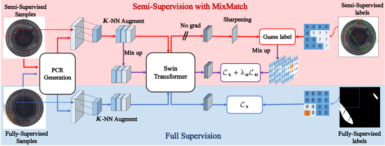
Figure 3: The overview of the training process of SemiREST. Note that in the unsupervised and supervised settings, only the lower part (shown in blue) is used and the red part, i.e., the semi-supervision is leveraged in the semi-supervised setting. Better view in color.

4 Experiments

In this section, extensive experiments are conducted to evaluate the proposed method, compared with a comprehensive collection of SOTA methods (Roth et al., 2022; Zavrtanik et al., 2021; Deng and Li, 2022), (Ristea et al., 2022; Liu et al., 2023a, b; Zhang et al., 2023b; Lei et al., 2023; Gudovskiy et al., 2022; Tien et al., 2023; Zhang et al., 2023a; Yao et al., 2023; Pang et al., 2021; Ding et al., 2022), on three well-acknowledged benchmarks, namely, the MVTec-AD (Bergmann et al., 2019) dataset, the BTAD (Mishra et al., 2021) dataset and the KolektorSDD2 dataset (Božič et al., 2021), respectively.

4.1 Three levels of supervision

First of all, let us clarify the experiment settings for the three kinds of supervision.

4.1.1 Unsupervised (Un) setting

The unsupervised setting is the mainstream in the AD literature, where only normal data can be accessed during training. However, discriminative models can be learned by generating synthetic anomalies. The involved algorithms are evaluated on the entire test set, including both normal and anomalous images.

4.1.2 Supervised (Sup) setting

In this scenario, a few anomaly training samples are available to improve the discriminative power of the algorithm. Following the popular setting described in (Zhang et al., 2023a), we randomly draw $10$ anomalous images with block-wise annotations from various types of defects to the train set and remove them from the test set. Note that synthetic anomalies can usually be used here for higher performance.

4.1.3 Semi-supervised (Semi) setting

The semi-supervised setting is the newly proposed supervision and is thus employed in this work only. The same $10$ anomalous images are used as training samples while the block labels of them are determined by the bounding-boxes which are defined in Equation 15. Note that in this case, all the blocks are annotated as either unknown or normal.

4.2 Implementation details

4.2.1 Hyper parameters

The layer-$2$ and layer-$3$ feature maps of the WideResnet-$50$ model (Zagoruyko and Komodakis, 2016) (pre-trained on ImageNet-1K) are concatenated with a proper scale adaptation and the yielded $d_{f}=1024$ “hyper-columns” are smoothed via average pooling in the ${3\times 3}$ neighborhoods. We set $\lambda_{\mathrm{PE}}=0.1$ to generate PCFs. For MVTec-AD (Bergmann et al., 2019) and BTAD (Mishra et al., 2021) datasets, we subsample $10\%$ of the PCFs to get the memory banks $\hat{\mathcal{M}}$, while the subsampling ratio for KolektorSDD2 (Božič et al., 2021) is $0.1\%$ considering the much larger training set of normal images. Our Swin Transformer model $\Psi_{\mathrm{Swin}}(\cdot)$ consists of $4$ blocks with patch size $\rho=1$, the window size is $8$ and the number of heads is set to $32$. The parameters of the focal loss ${\alpha_{x}}$, ${\alpha_{u}}$, ${\gamma_{x}}$ and ${\gamma_{u}}$ are set to $0.25$, $0.75$, $4$ and $4$ respectively. The sliding window $\mathbf{w}$ slides over the PCR tensor with a step $s=8$ and the window size is $\mu=32$. $a_{1}$ and $a_{2}$ are set to $0.5$ and $0.8$ respectively. To speed up training, we sample $p$ of sliding windows in $b_{1}$ normal images, $b_{2}$ simulated defective images, and $b_{3}$ true anomalous images at each training iteration. To compare the final prediction map $\Theta$ with the ground-truth label map, it is firstly upscaled to the same size as the ground-truth via bilinear interpolation and then smoothed using a Gaussian of kernel with ${\sigma}=4$, as it is done in (Roth et al., 2022).

The values of $lr$, $p$, $\epsilon^{+}$, $\epsilon^{-}$, $b_{1}$, $b_{2}$ and $b_{3}$ vary among different supervision conditions:

• Unsupervised setting: $lr=10^{-4}$, $p=1/4$, $\epsilon^{+}=50\%$, $\epsilon^{-}=8\%$, $b_{1}=4$, $b_{2}=2$ ($lr=3\times 10^{-4}$, $p=1/6$, $\epsilon^{+}=25\%$, $b_{2}=4$ for BTAD (Mishra et al., 2021)).

• Supervised setting: $lr=10^{-4}$, $p=1/4$, $\epsilon^{+}=25\%$, $\epsilon^{-}=8\%$, $b_{1}=2$, $b_{2}=2$ and $b_{3}=2$.

• Semi-supervised setting: $lr=3\times 10^{-5}$, $p=1/10$, $\epsilon^{+}=25\%$, $\epsilon^{-}=8\%$, $b_{1}=3$, $b_{2}=3$ and $b_{3}=2$ ($lr=3.125\times 10^{-5}$, $p=1/25$, $\epsilon^{+}=80\%$, $\epsilon^{-}=0\%$ for BTAD (Mishra et al., 2021)).

As to the semi-supervised learning, the hyperparameters $v$, $\alpha$, $\Gamma$ and $M$ are set to $50\%$, $25\%$, $0.5$ and $3$ respectively. The random noise for agumentation is set to $\boldsymbol{\delta}=e^{z},z\sim\mathcal{N}(0,0.2),z\in[\text{-}0.223,0.223]$. Following the MixMatch algorithm (Berthelot et al., 2019b), we linearly ramp up the unlabeled loss weight to $\lambda_{\mathit{u}}=5$ ($10$ for BTAD) over the first $400$ steps of training.

4.2.2 Train and inference time

The proposed method requires around $120$ ms to predict anomaly on a $512\times 512$ image. It takes $42$, $48$, and $56$ minutes to train the Swin Transformer model on MVTec-AD (Bergmann et al., 2019) with the unsupervised, semi-supervised, and supervised settings respectively.

4.3 Evaluation methods

In this work, the involved AD algorithms are measured comprehensively by three popular threshold-indeendent metrics: Pixel-AUROC, PRO (Bergmann et al., 2020) (per region overlap) and AP (Zavrtanik et al., 2021) (average precision). In specific, Pixel-AUROC is the area under the receiver operating characteristic curve at the pixel level. It is the most popular AD measuring method while fails to reflect the real performance difference between algorithms when a serious class imbalance exists. The PRO score, on the contrary, focuses on the anomaly pixels and treats the AD performance on each individual anomaly region equally. Consequently, the PRO metric is more robust to the class imbalance which is actually a common situation in most AD benchmarks. The AP (average precision) metric (Zavrtanik et al., 2021), as a conventional metric for semantic segmentation, is frequently adopted in recently proposed AD algorithms (Zavrtanik et al., 2021; Zhang et al., 2023a). It reflects the anomaly detection performance from a pixel-level perspective.

4.4 Results on MVTec-AD

MVTec-AD (Bergmann et al., 2019) is the most popular AD dataset with $5,354$ high-resolution color images belonging to $5$ texture categories and $10$ object categories. Each category contains a train set with only normal images and a test set with various kinds of defects as well as defect-free images. We conduct the experiments on this dataset within all three supervision conditions.

The unsupervised AD results of the comparing algorithms on MVTec-AD (Bergmann et al., 2019) are shown in Table 1. As shown in the table, our method achieves the highest average AP, average PRO and average pixel AUROC, for both texture and object categories and outperforms the unsupervised SOTA by $5.4\%$, $1.6\%$ and $1.0\%$ respectively. In specific, SemiREST ranks the first on $67\%$ ($10$ out of $15$) categories with AP metric and the “first-ranking” ratios for the PRO and Pixel-AUROC are $47\%$ and $80\%$.

In addition, Table 2 illustrates that with full supervision, SemiREST still ranks first for the average AD performance evaluated by using all three metrics. In particular, our method outperforms the supervised SOTAs by $5.8\%$ on AP, $0.4\%$ on PRO and $0.3\%$ on Pixel-AUROC. The “first-ranking” ratios of SemiREST in the supervised scenario are $47\%$, $67\%$ and $67\%$ one AP, PRO and Pixel-AUROC respectively.

Table 2 also reports the performances of our method with the bounding-box-determined semi-supervisions. It can be seen that the semi-supervised SemiREST performs very similarly to the fully-supervised SemiREST, thanks to the effective usage of the unlabeled blocks. In addition, even with much less annotation information, the semi-supervised SemiREST still beats the fully-supervised SOTA methods by large margins ($5.2\%$ for AP, $0.4\%$ for PRO and $0.3\%$ for Pixel-AUROC).

It is interesting to see that, with only synthetic defective samples, the unsupervised SemiREST remains the superiority to the supervised SOTA, with the AP and Pixel-AUROC metrics (see Table 1 and see Table 2). The proposed algorithm illustrates remarkably high generalization capacities.

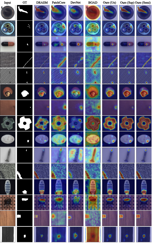
Figure 6: Qualitative results of our SemiREST on MVTec-AD, with the three levels of supervision: Un (unsupervised), Sup (supervised), and Semi (semi-supervised). Two unsupervised SOTA methods (PatchCore (Roth et al., 2022) and DRAEM (Zavrtanik et al., 2021)) and two SOTA methods with full supervision (DevNet (Pang et al., 2021) and BGAD (Yao et al., 2023)) are also involved in the comparison.

Readers can also find the qualitative results of the proposed method compared with other SOTA algorithms in Figure 6.

Category	PatchCore	DRAEM	RD	SSPCAB	NFAD	DMAD	SimpleNet	DeSTSeg	PyramidFlow	RD++	Ours (Un)
	(Roth et al., 2022)	(Zavrtanik et al., 2021)	(Deng and Li, 2022)	(Ristea et al., 2022)	(Yao et al., 2023)	(Liu et al., 2023a)	(Liu et al., 2023b)	(Zhang et al., 2023b)	(Lei et al., 2023)	(Tien et al., 2023)
Carpet	64.1/95.1/99.1	53.5/92.9/95.5	56.5/95.4/98.9	48.6/86.4/92.6	74.1/98.2/99.4	63.8/95.9/99.0	44.1/92.0/97.7	72.8/$\sim$/96.1	$\sim$/97.2/97.4	$\sim$/97.7/99.2	84.2/98.7/99.6
Grid	30.9/93.6/98.8	65.7/98.3/99.7	15.8/94.2/98.3	57.9/98.0/99.5	51.9/97.9/99.3	47.0/97.3/99.2	39.6/94.6/98.7	61.5/$\sim$/99.1	$\sim$/94.3/95.7	$\sim$/97.7/99.3	65.5/97.9/99.5
Leather	45.9/97.2/99.3	75.3/97.4/98.6	47.6/98.2/99.4	60.7/94.0/96.3	70.1/99.4/99.7	53.1/98.0/99.4	48.0/97.5/99.2	75.6/$\sim$/99.7	$\sim$/99.2/98.7	$\sim$/99.2/99.4	79.3/99.4/99.8
Tile	54.9/80.2/95.7	92.3/98.2/99.2	54.1/85.6/95.7	96.1/98.1/99.4	63.0/91.8/96.7	56.5/84.3/95.8	63.5/78.3/93.9	90.0/$\sim$/98.0	$\sim$/97.2/97.1	$\sim$/92.4/96.6	96.4/98.5/99.7
Wood	50.0/88.3/95.0	77.7/90.3/96.4	48.3/91.4/95.8	78.9/92.8/96.5	62.9/95.6/96.9	45.5/89.3/94.8	48.8/83.9/93.9	81.9/$\sim$/97.7	$\sim$/97.9/97.0	$\sim$/93.3/95.8	79.4/96.5/97.7
Average	49.2/90.9/97.6	72.9/95.4/97.9	44.5/93.0/97.6	68.4/93.9/96.9	64.4/96.6/98.4	53.2/93.0/97.6	48.8/89.3/96.7	76.4/$\sim$/98.1	$\sim$/97.2/97.2	$\sim$/96.1/98.1	81.0/98.2/99.3
Bottle	77.7/94.7/98.5	86.5/96.8/99.1	78.0/96.3/98.8	89.4/96.3/99.2	77.9/96.6/98.9	79.6/96.4/98.8	73.0/91.5/98.0	90.3/$\sim$/99.2	$\sim$/95.5/97.8	$\sim$/97.0/98.8	94.1/98.6/99.6
Cable	66.3/93.2/98.4	52.4/81.0/94.7	52.6/94.1/97.2	52.0/80.4/95.1	65.7/95.9/98.0	58.9/92.2/97.9	69.3/89.7/97.5	60.4/$\sim$/97.3	$\sim$/90.3/91.8	$\sim$/93.9/98.4	81.1/95.3/99.1
Capsule	44.7/94.8/99.0	49.4/82.7/94.3	47.2/95.5/98.7	46.4/92.5/90.2	58.7/96.0/99.2	42.2/91.6/98.1	44.7/92.8/98.9	56.3/$\sim$/99.1	$\sim$/98.3/98.6	$\sim$/96.4/98.8	57.2/96.9/98.8
Hazelnut	53.5/95.2/98.7	92.9/98.5/99.7	93.4/98.2/99.7	60.0/95.2/98.6	65.3/97.6/98.6	63.4/95.9/99.1	48.3/92.2/97.6	88.4/$\sim$/99.6	$\sim$/98.1/98.1	$\sim$/96.3/99.2	87.8/96.1/99.6
Metal nut	86.9/94.0/98.3	96.3/97.0/99.5	78.6/94.9/97.3	94.7/97.7/99.4	76.6/94.9/97.7	79.0/94.2/97.1	92.6/91.3/98.7	93.5/$\sim$/98.6	$\sim$/91.4/97.2	$\sim$/93.0/98.1	96.6/97.5/99.5
Pill	77.9/95.0/97.8	48.5/88.4/97.6	76.5/96.7/98.1	48.3/89.6/97.2	72.6/98.1/98.0	79.7/96.9/98.5	80.1/93.9/98.5	83.1/$\sim$/98.7	$\sim$/96.1/96.1	$\sim$/97.0/98.3	85.9/98.4/99.2
Screw	36.1/97.1/99.5	58.2/95.0/97.6	52.1/ 98.5/99.7	61.7/95.2/99.0	47.4/96.3/99.2	47.9/96.5/99.3	38.8/95.2/99.2	58.7/$\sim$/98.5	$\sim$/94.7/94.6	$\sim$/98.6/99.7	65.9/97.9/99.7
Toothbrush	38.3/89.4/98.6	44.7/85.6/98.1	51.1/92.3/99.1	39.3/85.5/97.3	38.8/92.3/98.7	71.4/91.5/99.3	51.7/88.7/98.6	75.2/$\sim$/99.3	$\sim$/97.9/98.5	$\sim$/94.2/99.1	74.5/96.2/99.5
Transistor	66.4/92.4/96.3	50.7/70.4/90.9	54.1/83.3/92.3	38.1/62.5/84.8	56.0/82.0/94.0	58.5/85.2/94.1	69.0/93.2/96.8	64.8/$\sim$/89.1	$\sim$/94.7/96.9	$\sim$/81.8/94.3	79.4/96.0/98.0
Zipper	62.8/95.8/98.9	81.5/96.8/98.8	57.5/95.3/98.3	76.4/95.2/98.4	56.0/95.7/98.6	50.1/93.8/97.9	60.0/91.2/97.8	85.2/$\sim$/99.1	$\sim$/95.4/96.6	$\sim$/96.3/98.8	90.2/98.9/99.7
Average	61.1/94.2/98.4	66.1/89.2/97.0	60.8/94.4/97.9	64.0/89.3/96.0	61.5/94.5/98.1	63.1/93.4/98.0	62.7/92.0/98.2	75.6/$\sim$/97.9	$\sim$/95.2/96.6	$\sim$/94.5/98.4	81.3/97.2/99.3
Total Average	57.1/93.1/98.1	68.4/91.3/97.3	55.4/93.9/97.8	65.5/90.8/96.3	62.5/95.2/98.2	59.8/93.3/97.9	58.1/91.1/97.7	75.8/$\sim$/97.9	$\sim$/95.9/96.8	$\sim$/95.0/98.3	81.2/97.5/99.3

Table 1: The comparison on the Average Precision (AP), Per-Region Overlap (PRO) and pixel AUROC metrics for zero-shot anomaly localization on the MVTec-AD dataset. The best accuracy in one comparison with the same data and metric condition is shown in red while the second one is shown in blue.

Category	PRN	BGAD	DevNet	DRA	Ours (Sup)	Ours (Semi)
	(Zhang et al., 2023a)	(Yao et al., 2023)	(Pang et al., 2021)	(Ding et al., 2022)
Carpet	82.0/97.0/99.0	83.2/98.9/99.6	45.7/85.8/97.2	52.3/92.2/98.2	89.1/99.1/99.7	88.9/99.1/99.7
Grid	45.7/95.9/98.4	59.2/98.7/98.4	25.5/79.8/87.9	26.8/71.5/86.0	66.4/97.0/99.4	71.5/98.5/99.7
Leather	69.7/99.2/99.7	75.5/99.5/99.8	8.1/88.5/94.2	5.6/84.0/93.8	81.7/99.7/99.9	82.0/99.6/99.9
Tile	96.5/98.2/99.6	94.0/97.9/99.3	52.3/78.9/92.7	57.6/81.5/92.3	96.9/98.9/99.7	96.6/98.7/99.7
Wood	82.6/95.9/97.8	78.7/96.8/98.0	25.1/75.4/86.4	22.7/69.7/82.9	88.7/97.9/99.2	86.2/97.1/98.6
Average	75.3/97.2/98.9	78.1/98.4/99.2	31.3/81.7/91.7	33.0/79.8/90.6	84.7/98.5/99.5	85.0/98.6/99.5
Bottle	92.3/97.0/99.4	87.1/97.1/99.3	51.5/83.5/93.9	41.2/77.6/91.3	93.6/98.5/99.5	93.6/98.4/99.5
Cable	78.9/97.2/98.8	81.4/97.7/98.5	36.0/80.9/88.8	34.7/77.7/86.6	89.5/95.9/99.2	86.5/96.3/99.3
Capsule	62.2/92.5/98.5	58.3/96.8/98.8	15.5/83.6/91.8	11.7/79.1/89.3	60.0/97.0/98.8	58.4/97.6/99.1
Hazelnut	93.8/97.4/99.7	82.4/98.6/99.4	22.1/83.6/91.1	22.5/86.9/89.6	92.2/98.3/99.8	86.0/97.3/99.7
Metal nut	98.0/95.8/99.7	97.3/96.8/99.6	35.6/76.9/77.8	29.9/76.7/79.5	99.1/98.2/99.9	98.3/98.1/99.8
Pill	91.3/97.2/99.5	92.1/98.7/99.5	14.6/69.2/82.6	21.6/77.0/84.5	86.1/98.9/99.3	89.6/98.9/99.5
Screw	44.9/92.4/97.5	55.3/96.8/99.3	1.4/31.1/60.3	5.0/30.1/54.0	72.1/98.8/99.8	67.9/98.6/99.8
Toothbrush	78.1/95.6/99.6	71.3/96.4/99.5	6.7/33.5/84.6	4.5/56.1/75.5	74.2/97.1/99.6	73.3/96.7/99.6
Transistor	85.6/94.8/98.4	82.3/97.1/97.9	6.4/39.1/56.0	11.0/49.0/79.1	85.5/97.8/98.6	86.4/97.9/98.6
Zipper	77.6/95.5/98.8	78.2/97.7/99.3	19.6/81.3/93.7	42.9/91.0/96.9	91.0/99.2/99.7	91.3/99.2/99.8
Average	80.3/95.5/99.0	78.6/97.4/99.1	20.9/66.3/82.1	22.5/70.1/82.6	84.3/98.0/99.4	83.2/97.9/99.5
Total Average	78.6/96.1/99.0	78.4/97.7/99.2	24.4/71.4/85.3	26.0/73.3/85.3	84.4/98.1/99.5	83.8/98.1/99.5

Table 2: The comparison on the Average Precision (AP), Per-Region Overlap (PRO) and pixel AUROC metrics for few-shot anomaly localization on the MVTec-AD dataset. The best accuracy in one comparison with the same data and metric condition is shown in red while the second one is shown in blue.

4.5 Results on BTAD

As a more challenging alternative to MVTec-AD, BTAD (Mishra et al., 2021) (beanTech Anomaly Detection) contains $2,830$ high-resolution color images of three industrial products. Each product includes normal images in the train set and the corresponding test set consists of both defective and defect-free images.

We further evaluate our algorithm on the BTAD dataset with those SOTA methods also reporting their results on this dataset. Table 3 shows that SemiREST achieves comparable performances to the unsupervised SOTA. Furthermore, as shown in Table 4, with full supervision, the proposed method surpasses SOTA methods by a large margin ($6.7\%$, $5.5\%$ and $0.3\%$) for all three metrics. Similarly to the situation of MVTec-AD, the semi-supervised SemiREST also obtains higher average performances than the supervised SOTA algorithms.

Category	PatchCore	DRAEM	SSPCAB	CFLOW	RD	PyramidFlow	NFAD	RD++	Ours (Un)
	(Roth et al., 2022)	(Zavrtanik et al., 2021)	(Ristea et al., 2022)	(Gudovskiy et al., 2022)	(Deng and Li, 2022)	(Lei et al., 2023)	(Yao et al., 2023)	(Tien et al., 2023)
01	47.1/78.4/96.5	17.0/61.4/91.5	18.1/62.8/92.4	39.6/60.1/94.8	49.3/72.8/95.7	$\sim$/$\sim$/97.4	46.7/76.6/96.7	$\sim$/73.2/96.2	52.4/83.9/97.5
02	56.3/54.0/94.9	23.3/39.0/73.4	15.8/28.6/65.6	65.5/56.9/93.9	66.1/55.8/96.0	$\sim$/$\sim$/97.6	59.2/57.9/96.4	$\sim$/71.3/96.4	63.1/61.5/96.5
03	51.2/96.4/99.2	17.2/84.3/96.3	5.0/71.0/92.4	56.8/97.9/99.5	45.1/98.8/99.0	$\sim$/$\sim$/98.1	62.8/98.8/99.7	$\sim$/87.4/99.7	50.9/98.8/99.7
Average	51.5/76.3/96.9	19.2/61.6/87.1	13.0/54.1/83.5	54.0/71.6/96.1	53.5/75.8/96.9	$\sim$/$\sim$/97.7	56.2/77.8/97.6	$\sim$/77.3/97.4	55.5/81.4/97.9

Table 3: Results of the AP, PRO and pixel AUROC metrics for unsupervised anomaly localization performance on BTAD. The best accuracy in one comparison with the same data and metric condition is shown in red while the second one is shown in blue.

Category	BGAD	PRN	Ours (Sup)	Ours (Semi)
	(Yao et al., 2023)	(Zhang et al., 2023a)
01	64.0/86.6/98.4	38.8/81.4/96.6	81.3/93.1/99.0	69.8/86.2/98.2
02	83.4/66.5/97.9	65.7/54.4/95.1	84.7/81.4/98.1	81.2/69.0/97.9
03	77.4/99.5/99.9	57.4/98.3/99.6	79.9/99.4/99.9	75.6/99.6/99.9
Average	74.9/84.2/98.7	54.0/78.0/97.1	82.0/91.3/99.0	75.5/84.9/98.7

Table 4: Results of the AP, PRO and pixel AUROC metrics for supervised and semi-supervised anomaly localization performance on BTAD. The best accuracy in one comparison with the same data and metric condition is shown in red while the second one is shown in blue.

4.6 Results on KolektorSDD2

KolektorSDD2 (Božič et al., 2021) dataset is designed for surface defect detection and includes various types of defects, such as scratches, minor spots, and surface imperfections. It comprises a training set with $246$ positive (defective) and $2,085$ negative (defect-free) images, as well as a test set with $110$ positive and $894$ negative images. We compare the performances of SemiREST with the SOTA results that are available in the literature. In the unsupervised setting, the algorithms are tested on the original test set. For the supervised and semi-supervised settings, a new training set is generated by combining all the normal training images and $10$ defective images which are randomly selected from the original training set.

As shown in Table 5, Our unsupervised performances beat those of SOTA methods by a large margin ($8.6\%$, $3.4\%$ and $1.8\%$ for AP, PRO and Pixel-AUROC, respectively). Under supervised and semi-supervised settings, our method also achieves better results. It is worth noting that the unsupervised SemiREST performs better than itself with full supervision and semi-supervision. This over-fitting phenomenon might be caused by the (unnecessarily) low sampling rate of defective images in training.

Method	AP	PRO	AUROC
PatchCore(Roth et al., 2022)	64.1	88.8	97.1
DRAEM(Zavrtanik et al., 2021)	39.1	67.9	85.6
SSPCAB(Ristea et al., 2022)	44.5	66.1	86.2
CFLOW(Gudovskiy et al., 2022)	46.0	93.8	97.4
RD(Deng and Li, 2022)	43.5	94.7	97.6
Ours(Un)	72.8	98.1	99.4
PRN(Zhang et al., 2023a)	72.5	94.9	97.6
Ours(Sup)	73.6	96.7	98.0
Ours(Semi)	72.1	97.5	99.1

Table 5: Results of anomaly localization performance on KolektorSDD2. The best accuracy in one comparison with the same data and metric condition is shown in red while the second one is shown in blue. Note that the upper sub-table shows the results obtained in the unsupervised condition and the lower part reports those with full-supervision or semi-supervision (only for SemiREST).

4.7 Analysis on weak labels

Recall that the main motivation of this paper is to reduce the labeling cost of AD tasks, we report the annotation time-consumption of the proposed two weak labels compared with pixel-level annotations.

To obtain the labeling time, the pixel labels, block labels and the bounding boxes of anomaly regions on a subset of MVTec-AD ($10$ defective image for each sub-category) are all manually annotated. Four master students majoring in computer vision complete the labeling task using a self-developed labeling tool, as shown in Figure 4. The annotators are asked to mimic the ground truth annotations shown in a sub-window of the GUI and the annotating time for each image is recorded.

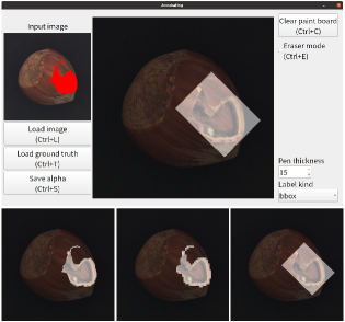
Figure 4: Our labeling tool and the yielded annotation maps. The upper part is the GUI window with the pixel-wise label map (red) displayed in the top-left corner. The lower part illustrates the annotations with three levels of fineness. They are, from left to right, pixel-wise labels, block-wise labels, and bounding-box labels, respectively.

The average annotation times of three kinds of labels are illustrated in Figure 5, along with the corresponding best AD performances (Pixel-AUROC, PRO, AP). According to the figure, one requires only around $5$ seconds for labeling bounding boxes and around $17$ seconds for generating block-wise labels, on one image. In contrast, the pixel-label consumes more than $32$ seconds for one image, while with consistently lower accuracy.

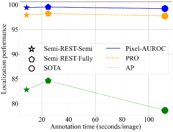
Figure 5: The per-image annotation costs (x-axis) of the three levels of anomaly labels, are shown as the pentagram (bounding-box label), pentagon (block-wise label) and circle (pixel-wise label) shapes. The y-axis stands for the AD performances with the three metrics, shown as blue-dot (Pixel-AUROC), orange-solid (PRO) and green-dashed (AP) lines.

4.8 Ablation study

In this section, the most influential modules of SemiREST are evaluated in the manner of an ablation study. The involved modules include: the usage of the PCF Section 3.1.1, the Bagging prediction of Swin Transformers Section 3.1.2, the $K$-NN augmentation of PCRs Section 3.2.1, the customized MixMatch algorithm Section 3.3 and the random dropout scheme Section 3.2.2, respectively. From Table 6 one can observe a consistent increase in the AD performance as more modules are added to the SemiREST model.

In addition, two element-wise distance functions (see Section 3.1.1), i.e., the absolute value of the difference (ABS) and the difference square (Square) are also compared in Table 6. According to the table, the square function outperforms the ABS function within unsupervised and semi-supervised settings where no real defective pixels are seen or labeled. The performance gain might be related to the “feature-selection” property of the square operation, which only focuses on the significant components of the residual vector. On the contrary, when the real defective samples are given for generating PCRs, more useful information can be maintained via the conservative ABS function.

Module						Performance
$\mathcal{S}(\cdot)$	PCF	Bagging	$K$-NN Augmentation	MixMatch	Random Dropout	Unsupervised	Supervised	Semi-supervised
Square						70.5/95.4/98.4	75.1/96.6/98.9	–
ABS						69.3/94.8/98.3	76.8/96.9/99.0	–
Square	$\checkmark$					72.4/95.8/98.9	76.4/96.6/99.0	–
Square	$\checkmark$	$\checkmark$				79.3/96.9/98.8	83.4/98.2/99.4	–
Square	$\checkmark$	$\checkmark$	$\checkmark$			81.2/97.5/99.3	84.4/98.2/99.5	80.7/97.5/99.3
Square	$\checkmark$	$\checkmark$	$\checkmark$	$\checkmark$		81.2/97.5/99.3	84.4/98.2/99.5	82.1/97.8/99.4
Square	$\checkmark$	$\checkmark$	$\checkmark$	$\checkmark$	$\checkmark$	81.2/97.5/99.3	84.4/98.2/99.5	83.8/98.1/99.5
ABS	$\checkmark$	$\checkmark$	$\checkmark$	$\checkmark$	$\checkmark$	76.4/96.3/98.7	84.9/98.3/99.5	83.2/98.0/99.3

Table 6: Ablation study results on MVTec-AD. Note that the semi-supervised SemiREST inherits the PCF feature, the bagging of swin transformer and $K$-NN augmentation modules from the fully-supervised version.

5 Conclusion

In this paper, we propose to solve the AD problem via block-wise classifications which require much less annotation effort than pixel-wise segmentation. To achieve this, a sliding vision transformer is employed to predict block labels, based on the smartly designed position-constrained residuals. The proposed bagging strategy of the Swin Transformers lead to the new SOTA accuracy on three well-known AD datasets. In addition, even cheaper bounding-box labels are proposed to further reduce the labeling time. Given only partially labeled normal regions, the customized MixMatch learning scheme successfully exploits the information of unlabeled regions and achieves the AD performances close to that with full-supervisions. The proposed SemiREST algorithm brings record-breaking AD performances to the literature while only requiring much coarser annotations or in short, our SemiREST is cheaper in annotation and better in accuracy.

Thus, SemiREST paves a novel way to reduce the annotation cost for AD problems while maintaining accuracy. According to the experiment of this work, the weak/semi-supervised setting seems a more practical alternative to the classic few-shot setting that directly limits the number of training images. In the future, we believe that better semi-supervised AD algorithms will be developed by exploiting more useful information from the unlabeled image regions.

Acknowledgements: This work was supported by National Key R&D Program of China (No. 2022ZD0118700) and the Fund for Less Developed Regions of the National Natural Science Foundation of China (Grant No. 61962027).

References

- Bae et al. (2022) Bae J, Lee JH, Kim S (2022) Image anomaly detection and localization with position and neighborhood information. arXiv preprint arXiv:221112634
- Bergmann et al. (2019) Bergmann P, Fauser M, Sattlegger D, Steger C (2019) Mvtec ad–a comprehensive real-world dataset for unsupervised anomaly detection. In: Proceedings of the IEEE/CVF conference on computer vision and pattern recognition, pp 9592–9600
- Bergmann et al. (2020) Bergmann P, Fauser M, Sattlegger D, Steger C (2020) Uninformed students: Student-teacher anomaly detection with discriminative latent embeddings. In: Proceedings of the IEEE/CVF conference on computer vision and pattern recognition, pp 4183–4192
- Bergmann et al. (2022) Bergmann P, Batzner K, Fauser M, Sattlegger D, Steger C (2022) Beyond dents and scratches: Logical constraints in unsupervised anomaly detection and localization. International Journal of Computer Vision 130(4):947–969
- Berthelot et al. (2019a) Berthelot D, Carlini N, Cubuk ED, Kurakin A, Sohn K, Zhang H, Raffel C (2019a) Remixmatch: Semi-supervised learning with distribution alignment and augmentation anchoring. arXiv preprint arXiv:191109785
- Berthelot et al. (2019b) Berthelot D, Carlini N, Goodfellow I, Papernot N, Oliver A, Raffel CA (2019b) Mixmatch: A holistic approach to semi-supervised learning. Advances in neural information processing systems 32
- Božič et al. (2021) Božič J, Tabernik D, Skočaj D (2021) Mixed supervision for surface-defect detection: From weakly to fully supervised learning. Computers in Industry 129:103459
- Breiman (1996) Breiman L (1996) Bagging predictors. Machine learning 24:123–140
- Cao et al. (2023a) Cao H, Wang Y, Chen J, Jiang D, Zhang X, Tian Q, Wang M (2023a) Swin-unet: Unet-like pure transformer for medical image segmentation. In: Computer Vision–ECCV 2022 Workshops: Tel Aviv, Israel, October 23–27, 2022, Proceedings, Part III, Springer, pp 205–218
- Cao et al. (2023b) Cao Y, Xu X, Liu Z, Shen W (2023b) Collaborative discrepancy optimization for reliable image anomaly localization. IEEE Transactions on Industrial Informatics pp 1–10, DOI 10.1109/TII.2023.3241579
- Chen et al. (2022) Chen Y, Tian Y, Pang G, Carneiro G (2022) Deep one-class classification via interpolated gaussian descriptor. In: Proceedings of the AAAI Conference on Artificial Intelligence, vol 36, pp 383–392
- Cheng et al. (2018) Cheng B, Wei Y, Shi H, Feris R, Xiong J, Huang T (2018) Revisiting rcnn: On awakening the classification power of faster rcnn. In: Proceedings of the European conference on computer vision (ECCV), pp 453–468
- Dai et al. (2021) Dai X, Chen Y, Xiao B, Chen D, Liu M, Yuan L, Zhang L (2021) Dynamic head: Unifying object detection heads with attentions. In: Proceedings of the IEEE/CVF conference on computer vision and pattern recognition, pp 7373–7382
- Defard et al. (2021) Defard T, Setkov A, Loesch A, Audigier R (2021) Padim: a patch distribution modeling framework for anomaly detection and localization. In: Pattern Recognition. ICPR International Workshops and Challenges: Virtual Event, January 10–15, 2021, Proceedings, Part IV, Springer, pp 475–489
- Dehaene and Eline (2020) Dehaene D, Eline P (2020) Anomaly localization by modeling perceptual features. arXiv preprint arXiv:200805369
- Deng and Li (2022) Deng H, Li X (2022) Anomaly detection via reverse distillation from one-class embedding. In: Proceedings of the IEEE/CVF Conference on Computer Vision and Pattern Recognition, pp 9737–9746
- Deng et al. (2009) Deng J, Dong W, Socher R, Li LJ, Li K, Fei-Fei L (2009) Imagenet: A large-scale hierarchical image database. In: 2009 IEEE conference on computer vision and pattern recognition, Ieee, pp 248–255
- Ding et al. (2022) Ding C, Pang G, Shen C (2022) Catching both gray and black swans: Open-set supervised anomaly detection. In: Proceedings of the IEEE/CVF Conference on Computer Vision and Pattern Recognition, pp 7388–7398
- Dinh et al. (2014) Dinh L, Krueger D, Bengio Y (2014) Nice: Non-linear independent components estimation. arXiv preprint arXiv:14108516
- Dinh et al. (2016) Dinh L, Sohl-Dickstein J, Bengio S (2016) Density estimation using real nvp. arXiv preprint arXiv:160508803
- Dong et al. (2021) Dong B, Zeng F, Wang T, Zhang X, Wei Y (2021) Solq: Segmenting objects by learning queries. Advances in Neural Information Processing Systems 34:21898–21909
- Dosovitskiy et al. (2021) Dosovitskiy A, Beyer L, Kolesnikov A, Weissenborn D, Zhai X, Unterthiner T, Dehghani M, Minderer M, Heigold G, Gelly S, et al. (2021) An image is worth 16x16 words: Transformers for image recognition at scale. In: International Conference on Learning Representations
- Gao et al. (2022) Gao L, Zhang J, Yang C, Zhou Y (2022) Cas-vswin transformer: A variant swin transformer for surface-defect detection. Computers in Industry 140:103689
- Gudovskiy et al. (2022) Gudovskiy D, Ishizaka S, Kozuka K (2022) Cflow-ad: Real-time unsupervised anomaly detection with localization via conditional normalizing flows. In: Proceedings of the IEEE/CVF Winter Conference on Applications of Computer Vision, pp 98–107
- Hatamizadeh et al. (2022) Hatamizadeh A, Nath V, Tang Y, Yang D, Roth HR, Xu D (2022) Swin unetr: Swin transformers for semantic segmentation of brain tumors in mri images. In: Brainlesion: Glioma, Multiple Sclerosis, Stroke and Traumatic Brain Injuries: 7th International Workshop, BrainLes 2021, Held in Conjunction with MICCAI 2021, Virtual Event, September 27, 2021, Revised Selected Papers, Part I, Springer, pp 272–284
- Haynes et al. (2012) Haynes D, Corns S, Venayagamoorthy GK (2012) An exponential moving average algorithm. In: 2012 IEEE Congress on Evolutionary Computation, IEEE, pp 1–8
- He et al. (2022) He K, Chen X, Xie S, Li Y, Dollár P, Girshick R (2022) Masked autoencoders are scalable vision learners. In: Proceedings of the IEEE/CVF Conference on Computer Vision and Pattern Recognition, pp 16000–16009
- Hou et al. (2021) Hou J, Zhang Y, Zhong Q, Xie D, Pu S, Zhou H (2021) Divide-and-assemble: Learning block-wise memory for unsupervised anomaly detection. In: Proceedings of the IEEE/CVF International Conference on Computer Vision, pp 8791–8800
- Hsu et al. (2019) Hsu CC, Hsu KJ, Tsai CC, Lin YY, Chuang YY (2019) Weakly supervised instance segmentation using the bounding box tightness prior. Advances in Neural Information Processing Systems 32
- Huang et al. (2022) Huang C, Guan H, Jiang A, Zhang Y, Spratling M, Wang YF (2022) Registration based few-shot anomaly detection. In: Computer Vision–ECCV 2022: 17th European Conference, Tel Aviv, Israel, October 23–27, 2022, Proceedings, Part XXIV, Springer, pp 303–319
- Huang et al. (2021) Huang S, Lu Z, Cheng R, He C (2021) Fapn: Feature-aligned pyramid network for dense image prediction. In: Proceedings of the IEEE/CVF international conference on computer vision, pp 864–873
- Huang et al. (2020) Huang Y, Qiu C, Yuan K (2020) Surface defect saliency of magnetic tile. The Visual Computer 36:85–96
- Kervadec et al. (2020) Kervadec H, Dolz J, Wang S, Granger E, Ayed IB (2020) Bounding boxes for weakly supervised segmentation: Global constraints get close to full supervision. In: Medical imaging with deep learning, PMLR, pp 365–381
- Kim et al. (2022) Kim D, Park C, Cho S, Lee S (2022) Fapm: Fast adaptive patch memory for real-time industrial anomaly detection. arXiv preprint arXiv:221107381
- Kingma and Dhariwal (2018) Kingma DP, Dhariwal P (2018) Glow: Generative flow with invertible 1x1 convolutions. Advances in neural information processing systems 31
- Lee et al. (2021) Lee J, Yi J, Shin C, Yoon S (2021) Bbam: Bounding box attribution map for weakly supervised semantic and instance segmentation. In: Proceedings of the IEEE/CVF conference on computer vision and pattern recognition, pp 2643–2652
- Lei et al. (2023) Lei J, Hu X, Wang Y, Liu D (2023) Pyramidflow: High-resolution defect contrastive localization using pyramid normalizing flow. In: Proceedings of the IEEE/CVF Conference on Computer Vision and Pattern Recognition (CVPR), pp 14143–14152
- Li et al. (2021) Li CL, Sohn K, Yoon J, Pfister T (2021) Cutpaste: Self-supervised learning for anomaly detection and localization. In: Proceedings of the IEEE/CVF Conference on Computer Vision and Pattern Recognition, pp 9664–9674
- Li et al. (2022) Li F, Zhang H, Liu S, Zhang L, Ni LM, Shum HY, et al. (2022) Mask dino: Towards a unified transformer-based framework for object detection and segmentation. arXiv preprint arXiv:220602777
- Liang et al. (2022) Liang T, Chu X, Liu Y, Wang Y, Tang Z, Chu W, Chen J, Ling H (2022) Cbnet: A composite backbone network architecture for object detection. IEEE Transactions on Image Processing 31:6893–6906
- Lin et al. (2017) Lin TY, Goyal P, Girshick R, He K, Dollár P (2017) Focal loss for dense object detection. In: Proceedings of the IEEE international conference on computer vision, pp 2980–2988
- Liu et al. (2023a) Liu W, Chang H, Ma B, Shan S, Chen X (2023a) Diversity-measurable anomaly detection. In: Proceedings of the IEEE/CVF Conference on Computer Vision and Pattern Recognition (CVPR), pp 12147–12156
- Liu et al. (2021) Liu Z, Lin Y, Cao Y, Hu H, Wei Y, Zhang Z, Lin S, Guo B (2021) Swin transformer: Hierarchical vision transformer using shifted windows. In: Proceedings of the IEEE/CVF international conference on computer vision, pp 10012–10022
- Liu et al. (2022) Liu Z, Hu H, Lin Y, Yao Z, Xie Z, Wei Y, Ning J, Cao Y, Zhang Z, Dong L, Wei F, Guo B (2022) Swin transformer v2: Scaling up capacity and resolution. In: Proceedings of the IEEE/CVF Conference on Computer Vision and Pattern Recognition (CVPR), pp 12009–12019
- Liu et al. (2023b) Liu Z, Zhou Y, Xu Y, Wang Z (2023b) Simplenet: A simple network for image anomaly detection and localization. In: Proceedings of the IEEE/CVF Conference on Computer Vision and Pattern Recognition (CVPR), pp 20402–20411
- Liznerski et al. (2021) Liznerski P, Ruff L, Vandermeulen RA, Franks BJ, Kloft M, Muller KR (2021) Explainable deep one-class classification. In: International Conference on Learning Representations, URL https://openreview.net/forum?id=A5VV3UyIQz
- Loshchilov and Hutter (2019) Loshchilov I, Hutter F (2019) Decoupled weight decay regularization. In: International Conference on Learning Representations
- Massoli et al. (2021) Massoli FV, Falchi F, Kantarci A, Akti Ş, Ekenel HK, Amato G (2021) Mocca: Multilayer one-class classification for anomaly detection. IEEE Transactions on Neural Networks and Learning Systems 33(6):2313–2323
- Mishra et al. (2021) Mishra P, Verk R, Fornasier D, Piciarelli C, Foresti GL (2021) Vt-adl: A vision transformer network for image anomaly detection and localization. In: 2021 IEEE 30th International Symposium on Industrial Electronics (ISIE), IEEE, pp 01–06
- Ni et al. (2021) Ni X, Ma Z, Liu J, Shi B, Liu H (2021) Attention network for rail surface defect detection via consistency of intersection-over-union (iou)-guided center-point estimation. IEEE Transactions on Industrial Informatics 18(3):1694–1705
- Niu et al. (2021) Niu S, Li B, Wang X, Peng Y (2021) Region-and strength-controllable gan for defect generation and segmentation in industrial images. IEEE Transactions on Industrial Informatics 18(7):4531–4541
- Pang et al. (2021) Pang G, Ding C, Shen C, Hengel Avd (2021) Explainable deep few-shot anomaly detection with deviation networks. arXiv preprint arXiv:210800462
- Ristea et al. (2022) Ristea NC, Madan N, Ionescu RT, Nasrollahi K, Khan FS, Moeslund TB, Shah M (2022) Self-supervised predictive convolutional attentive block for anomaly detection. In: Proceedings of the IEEE/CVF Conference on Computer Vision and Pattern Recognition, pp 13576–13586
- Roth et al. (2022) Roth K, Pemula L, Zepeda J, Schölkopf B, Brox T, Gehler P (2022) Towards total recall in industrial anomaly detection. In: Proceedings of the IEEE/CVF Conference on Computer Vision and Pattern Recognition, pp 14318–14328
- Rudolph et al. (2021) Rudolph M, Wandt B, Rosenhahn B (2021) Same same but differnet: Semi-supervised defect detection with normalizing flows. In: Proceedings of the IEEE/CVF winter conference on applications of computer vision, pp 1907–1916
- Ruff et al. (2018) Ruff L, Vandermeulen R, Goernitz N, Deecke L, Siddiqui SA, Binder A, Müller E, Kloft M (2018) Deep one-class classification. In: International conference on machine learning, PMLR, pp 4393–4402
- Russakovsky et al. (2015) Russakovsky O, Deng J, Su H, Krause J, Satheesh S, Ma S, Huang Z, Karpathy A, Khosla A, Bernstein M, et al. (2015) Imagenet large scale visual recognition challenge. International journal of computer vision 115:211–252
- Saiku et al. (2022) Saiku R, Sato J, Yamada T, Ito K (2022) Enhancing anomaly detection performance and acceleration. IEEJ Journal of Industry Applications 11(4):616–622
- Salehi et al. (2021) Salehi M, Sadjadi N, Baselizadeh S, Rohban MH, Rabiee HR (2021) Multiresolution knowledge distillation for anomaly detection. In: Proceedings of the IEEE/CVF conference on computer vision and pattern recognition, pp 14902–14912
- Scholkopf et al. (2000) Scholkopf B, Williamson R, Smola A, Shawe-Taylor J, Platt J, et al. (2000) Support vector method for novelty detection. Advances in neural information processing systems 12(3):582–588
- Schölkopf et al. (2001) Schölkopf B, Platt JC, Shawe-Taylor J, Smola AJ, Williamson RC (2001) Estimating the support of a high-dimensional distribution. Neural computation 13(7):1443–1471
- Shi et al. (2021) Shi Y, Yang J, Qi Z (2021) Unsupervised anomaly segmentation via deep feature reconstruction. Neurocomputing 424:9–22
- Shorten and Khoshgoftaar (2019) Shorten C, Khoshgoftaar TM (2019) A survey on image data augmentation for deep learning. Journal of big data 6(1):1–48
- Sohn et al. (2020) Sohn K, Berthelot D, Carlini N, Zhang Z, Zhang H, Raffel CA, Cubuk ED, Kurakin A, Li CL (2020) Fixmatch: Simplifying semi-supervised learning with consistency and confidence. Advances in neural information processing systems 33:596–608
- Srivastava et al. (2014) Srivastava N, Hinton G, Krizhevsky A, Sutskever I, Salakhutdinov R (2014) Dropout: a simple way to prevent neural networks from overfitting. The journal of machine learning research 15(1):1929–1958
- Tabernik et al. (2020) Tabernik D, Šela S, Skvarč J, Skočaj D (2020) Segmentation-based deep-learning approach for surface-defect detection. Journal of Intelligent Manufacturing 31(3):759–776
- Tailanian et al. (2022) Tailanian M, Pardo Á, Musé P (2022) U-flow: A u-shaped normalizing flow for anomaly detection with unsupervised threshold. arXiv preprint arXiv:221112353
- Tao et al. (2022) Tao X, Zhang D, Ma W, Hou Z, Lu Z, Adak C (2022) Unsupervised anomaly detection for surface defects with dual-siamese network. IEEE Transactions on Industrial Informatics 18(11):7707–7717
- Tien et al. (2023) Tien TD, Nguyen AT, Tran NH, Huy TD, Duong ST, Nguyen CDT, Truong SQH (2023) Revisiting reverse distillation for anomaly detection. In: Proceedings of the IEEE/CVF Conference on Computer Vision and Pattern Recognition (CVPR), pp 24511–24520
- Üzen et al. (2022) Üzen H, Türkoğlu M, Yanikoglu B, Hanbay D (2022) Swin-mfinet: Swin transformer based multi-feature integration network for detection of pixel-level surface defects. Expert Systems with Applications 209:118269
- Wang et al. (2022a) Wang CY, Bochkovskiy A, Liao HYM (2022a) Yolov7: Trainable bag-of-freebies sets new state-of-the-art for real-time object detectors. arXiv preprint arXiv:220702696
- Wang et al. (2022b) Wang W, Bao H, Dong L, Bjorck J, Peng Z, Liu Q, Aggarwal K, Mohammed OK, Singhal S, Som S, et al. (2022b) Image as a foreign language: Beit pretraining for all vision and vision-language tasks. arXiv preprint arXiv:220810442
- Wang et al. (2022c) Wang W, Dai J, Chen Z, Huang Z, Li Z, Zhu X, Hu X, Lu T, Lu L, Li H, et al. (2022c) Internimage: Exploring large-scale vision foundation models with deformable convolutions. arXiv preprint arXiv:221105778
- Wang et al. (2023) Wang Y, Chen H, Heng Q, Hou W, Fan Y, Wu Z, Wang J, Savvides M, Shinozaki T, Raj B, Schiele B, Xie X (2023) Freematch: Self-adaptive thresholding for semi-supervised learning. In: The Eleventh International Conference on Learning Representations, URL https://openreview.net/forum?id=PDrUPTXJI_A
- Wu et al. (2021) Wu JC, Chen DJ, Fuh CS, Liu TL (2021) Learning unsupervised metaformer for anomaly detection. In: Proceedings of the IEEE/CVF International Conference on Computer Vision, pp 4369–4378
- Xie et al. (2023) Xie G, Wang J, Liu J, Jin Y, Zheng F (2023) Pushing the limits of fewshot anomaly detection in industry vision: Graphcore. In: The Eleventh International Conference on Learning Representations, URL https://openreview.net/forum?id=xzmqxHdZAwO
- Xu et al. (2021) Xu M, Zhang Z, Hu H, Wang J, Wang L, Wei F, Bai X, Liu Z (2021) End-to-end semi-supervised object detection with soft teacher. In: Proceedings of the IEEE/CVF International Conference on Computer Vision, pp 3060–3069
- Yang et al. (2023) Yang M, Wu P, Feng H (2023) Memseg: A semi-supervised method for image surface defect detection using differences and commonalities. Engineering Applications of Artificial Intelligence 119:105835
- Yang et al. (2022) Yang S, Xiao W, Zhang M, Guo S, Zhao J, Shen F (2022) Image data augmentation for deep learning: A survey. arXiv preprint arXiv:220408610
- Yao et al. (2023) Yao X, Li R, Zhang J, Sun J, Zhang C (2023) Explicit boundary guided semi-push-pull contrastive learning for supervised anomaly detection. In: Proceedings of the IEEE/CVF Conference on Computer Vision and Pattern Recognition (CVPR), pp 24490–24499
- Yi and Yoon (2020) Yi J, Yoon S (2020) Patch svdd: Patch-level svdd for anomaly detection and segmentation. In: Proceedings of the Asian Conference on Computer Vision
- Yu et al. (2021) Yu J, Zheng Y, Wang X, Li W, Wu Y, Zhao R, Wu L (2021) Fastflow: Unsupervised anomaly detection and localization via 2d normalizing flows. arXiv preprint arXiv:211107677
- Yun et al. (2019) Yun S, Han D, Oh SJ, Chun S, Choe J, Yoo Y (2019) Cutmix: Regularization strategy to train strong classifiers with localizable features. In: Proceedings of the IEEE/CVF international conference on computer vision, pp 6023–6032
- Zagoruyko and Komodakis (2016) Zagoruyko S, Komodakis N (2016) Wide residual networks. arXiv preprint arXiv:160507146
- Zavrtanik et al. (2021) Zavrtanik V, Kristan M, Skočaj D (2021) Draem-a discriminatively trained reconstruction embedding for surface anomaly detection. In: Proceedings of the IEEE/CVF International Conference on Computer Vision, pp 8330–8339
- Zhang et al. (2021a) Zhang G, Cui K, Hung TY, Lu S (2021a) Defect-gan: High-fidelity defect synthesis for automated defect inspection. In: Proceedings of the IEEE/CVF Winter Conference on Applications of Computer Vision, pp 2524–2534
- Zhang et al. (2018) Zhang H, Cisse M, Dauphin YN, Lopez-Paz D (2018) mixup: Beyond empirical risk minimization. In: International Conference on Learning Representations, URL https://openreview.net/forum?id=r1Ddp1-Rb
- Zhang et al. (2023a) Zhang H, Wu Z, Wang Z, Chen Z, Jiang YG (2023a) Prototypical residual networks for anomaly detection and localization. In: Proceedings of the IEEE/CVF Conference on Computer Vision and Pattern Recognition (CVPR), pp 16281–16291
- Zhang et al. (2021b) Zhang J, Su H, Zou W, Gong X, Zhang Z, Shen F (2021b) Cadn: a weakly supervised learning-based category-aware object detection network for surface defect detection. Pattern Recognition 109:107571
- Zhang et al. (2022) Zhang K, Wang B, Kuo CCJ (2022) Pedenet: Image anomaly localization via patch embedding and density estimation. Pattern Recognition Letters 153:144–150
- Zhang et al. (2023b) Zhang X, Li S, Li X, Huang P, Shan J, Chen T (2023b) Destseg: Segmentation guided denoising student-teacher for anomaly detection. In: Proceedings of the IEEE/CVF Conference on Computer Vision and Pattern Recognition (CVPR), pp 3914–3923
- Zhu et al. (2022) Zhu H, Kang Y, Zhao Y, Yan X, Zhang J (2022) Anomaly detection for surface of laptop computer based on patchcore gan algorithm. In: 2022 41st Chinese Control Conference (CCC), IEEE, pp 5854–5858
- Zhu and Goldberg (2009) Zhu X, Goldberg AB (2009) Introduction to semi-supervised learning. Synthesis lectures on artificial intelligence and machine learning 3(1):1–130
- Zong et al. (2018) Zong B, Song Q, Min MR, Cheng W, Lumezanu C, Cho D, Chen H (2018) Deep autoencoding gaussian mixture model for unsupervised anomaly detection. In: International conference on learning representations