Compiling Quantum Circuits for Dynamically Field-Programmable Neutral Atoms Array Processors

Abstract

Dynamically field-programmable qubit arrays (DPQA) have recently emerged as a promising platform for quantum information processing. In DPQA, atomic qubits are selectively loaded into arrays of optical traps that can be reconfigured during the computation itself. Leveraging qubit transport and parallel, entangling quantum operations, different pairs of qubits, even those initially far away, can be entangled at different stages of the quantum program execution. Such reconfigurability and non-local connectivity present new challenges for compilation, especially in the layout synthesis step which places and routes the qubits and schedules the gates. In this paper, we consider a DPQA architecture that contains multiple arrays and supports 2D array movements, representing cutting-edge experimental platforms. Within this architecture, we discretize the state space and formulate layout synthesis as a satisfactory modulo theories problem, which can be solved by existing solvers optimally in terms of circuit depth. For a set of benchmark circuits generated by random graphs with complex connectivities, our compiler OLSQ-DPQA reduces the number of two-qubit entangling gates on small problem instances by 1.7x compared to optimal compilation results on a fixed planar architecture. To further improve scalability and practicality of the method, we introduce a greedy heuristic inspired by the iterative peeling approach in classical integrated circuit routing. Using a hybrid approach that combined the greedy and optimal methods, we demonstrate that our DPQA-based compiled circuits feature reduced scaling overhead compared to a grid fixed architecture, resulting in 5.1X less two-qubit gates for 90 qubit quantum circuits. These methods enable programmable, complex quantum circuits with neutral atom quantum computers, as well as informing both future compilers and future hardware choices.

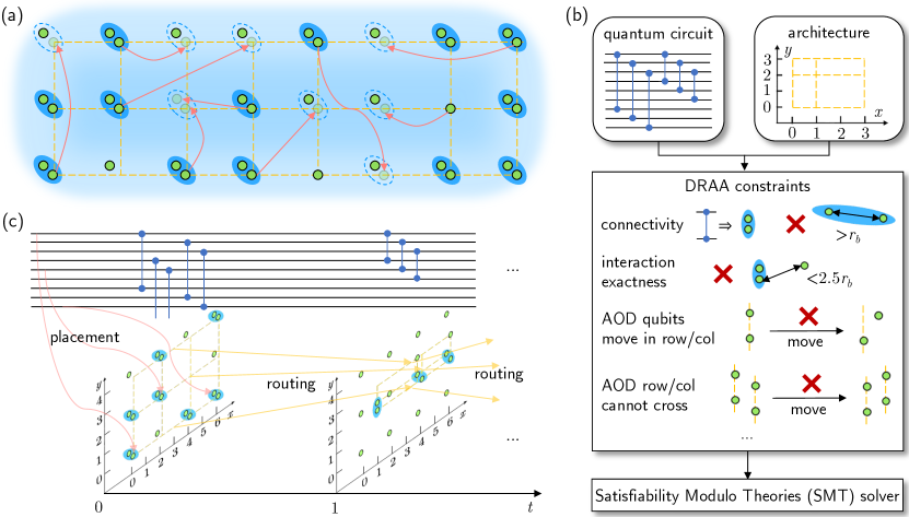
Figure 1: Compiling quantum circuits to dynamically field-programmable qubit arrays (DPQA). (a) Non-local connectivity of DPQA. Atoms are kept in traps generated by a 2D acousto-optic deflector (AOD, dashed grid) and a spatial light modulator (SLM, all others). Entangling two-qubit gates are enabled by a Rydberg laser illuminating the plane (glow). Only when two atoms are within the Rydberg blockade range $r_{b}$ can they perform an entangling gate (pairs in colored ovals). We can change the location of AOD atoms, and transfer atoms between AOD and SLM traps [2] in the middle of computation (each arrow corresponding to some AOD reconfiguration). Through such reconfigurations, new non-local connectivities are established (oval dashes), i.e., different pairs of atoms can now perform entangling gates. (b) Our compilation approach. The input consists of the quantum circuit to execute and the DPQA architecture specification, e.g., how large the plane is and how many AOD rows and columns we can have. The compiled instructions have to respect the constraints of DPQA. For example, when a two-qubit gate is executed, the two qubits should be closer than $r_{b}$ and there cannot be another qubit nearby. Also, all traps in the same AOD row/column move together and must stay in the same order from the beginning to the end of the process. We formulate all the constraints to a satisfiability modulo theories (SMT) model and use an existing SMT solver to find solutions, with which we can derive valid DPQA instructions to run the circuit. (c) Structure of compiled results. We discretize space by prescribing interaction sites shown as the proximity of integer points in the plane. The distance between sites is sufficient to suppress Rydberg interaction strengths [3, 4] so the two-qubit entangling gates can only take place within sites. Our compiler places the qubits in the quantum circuit to atoms in SLM or AOD at a specific interaction site in the beginning of execution. We discretize time by setting stages when two-qubit gates are performed. After each stage, some AOD movements and atom transfers serve as routing for the gates executed at the next stage.

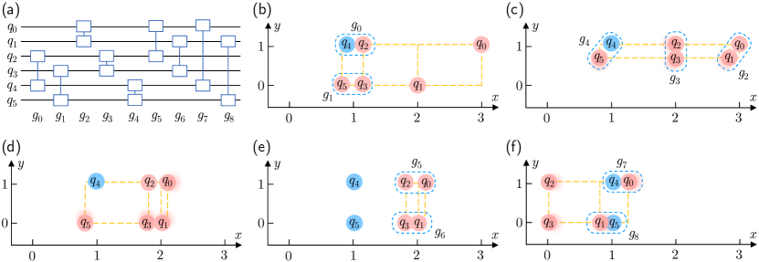
Figure 2: A compiled example. (a) The quantum circuit to compile. (b) Stage 0. Qubits are loaded to the corresponding traps before this stage: blue qubits are in SLM, red qubits are in AOD. An AOD trap sits at every intersection of the AOD columns and rows (x and y dashed lines). At stage 0, $(q_{4},q_{2})$ and $(q_{5},q_{3})$ are at same sites to enable a Rydberg interaction. Thus, two gates (oval dashes) $g_{0}$ and $g_{1}$ are applied to these two pairs of qubits. After stage 0, the movement shifts the lower AOD row from $y=0$ to $1$ and the middle two columns go from $x=1$ and $2$ to $x=2$ and $3$, respectively. (c) Stage 1. Shadows of qubits indicate the direction of the movements from the previous stage to the current one. (d) The moment after the movement between stage 1 and 2. (e) Stage 2. $q_{5}$ is transferred from AOD to SLM (red to blue) after the movement and before stage 2 by shifting the leftmost AOD column to align with the SLM trap at $(1,0)$ and then turning off this column. (f) Stage 3 finishing the circuit execution.

1 Introduction

The power of quantum computing relies on the ability to generate large-scale entanglement among qubits. Entangling operations such as two-qubit gates requires qubits to interact, which often confines gate connectivity to be geometrically local. Since superconducting quantum processors are fabricated on a 2D plane [5, 6, 7], the qubit connectivities are planar with a low node degree for practical reasons [8]. For small trapped-ion quantum processors [9, 10], the connectivity is all-to-all. However, it is challenging to maintain this feature when scaling up to multiple ion traps [11], although exciting progress is being made [12].

Recently, neutral atoms trapped in arrays of optical tweezers have become a leading experimental platform for quantum computing. These systems are readily scaled to large numbers: Ebadi et al. [13] have operated up to 289 neutral atom qubits, and significant increases in system size are expected to continue. Neutral atoms have recently also reached state-of-the-art fidelities: Evered et al. [4] realized parallel CZ gates on 60 qubits with fidelity $99.5\%$. Moreover, Bluvstein et al. [3] have demonstrated dynamically field-programmable qubit arrays (DPQA) where the qubit connectivity can be reconfigured dynamically during the computation itself, as illustrated by Fig. 1a.

DPQA opens the field up to new opportunities for running quantum circuits with non-local connectivities and a high degree of parallelism. However, in addition to its flexibility, there are hardware constraints, as shown in Fig. 1b. In the compilation flow of quantum computing, layout synthesis (Appendix B) places the qubits and routes them to execute the gates at the appropriate time steps, as depicted in Fig. 1c. Quantum layout synthesis has been studied for years [14, 15, 16, 17, 18, 19, 20, 21, 22, 23, 24, 25, 26, 27, 28, 29, 30, 31, 32, 33], but no previous compiler can fully leverage the reconfigurability and non-local connectivity of DPQA while conforming to all its constraints. Realizing a compiler for DPQA is an outstanding challenge that would enable unique opportunities in quantum computing with such a flexible architecture.

In this work, we realize layout synthesis of complex quantum circuits for neutral atom hardware in a compiler OLSQ-DPQA (optimal layout synthesizer of quantum circuits for DPQA). We encode states of the architecture in discrete variables specifying the location of qubits and the scheduling of gates. Based on these variables, we express constraints of DPQA with first-order logic and integer relations. Then, we use a satisfiability modulo theories (SMT) solver to derive valid variable assignments under the constraints yielding valid DPQA instructions to execute circuits.

The manuscript is organized as follows. In Section 2, we review the DPQA architecture, especially its constraints. In Section 3, we introduce the discrete variables that encode the state of DPQA in the computation spacetime. Section 4 explains how the constraints are constructed in SMT and how to invoke SMT solvers to derive optimal solutions with respect to circuit depth. In Section 5, we introduce a hybrid method including a greedy heuristic to accelerate the compilation and scale it to large sizes. We demonstrate the effectiveness of our compiler by comparing the results of both optimal and optimal-greedy hybrid approaches to fixed planar architectures using state-of-the-art compilers. Finally, in Section 6, we conclude the paper and provide future outlooks.

2 DPQA Architecture Description

In DPQA, every atom encodes a qubit, and they are held in optical traps. A spatial light modulator (SLM) generates some of the traps. These SLM-generated traps are stationary just like quantum registers in a fixed architecture, but can be placed in arbitrary locations [34, 35, 36]. However, there are also mobile traps [2] generated by a crossed 2D acousto-optic deflector (AOD) are represented by the dashed grid in Fig. 1a [37, 38]. If two atoms are within a certain Rydberg blockade range $r_{b}$, we can apply an entangling two-qubit gate on the pair with a so-called Rydberg laser [39, 40, 4]. In fact, the laser illuminates the whole plane where atoms are kept, so all pairs of qubits that are within distance $r_{b}$ perform two-qubit gates in parallel (pairs in colored ovals in Fig. 1a) [3].

Different configurations, i.e., different locations of AOD rows and columns, lead to different qubit connectivities. In principle, we can couple any AOD qubit $q$ at $(x_{q},y_{q})$ and any SLM qubit $q^{\prime}$ at $(x_{q^{\prime}},y_{q^{\prime}})$ by moving $q$ to $q^{\prime}$ by a distance roughly $(x_{q^{\prime}}-x_{q},y_{q^{\prime}}-y_{q})$. Also, we can bring adjacent AOD rows/columns close together to couple qubits in these rows/columns. The dashed ovals in Fig. 1a correspond to some of these potential couplings that some AOD reconfigurations (arrows, not necessarily simultaneously) can achieve.

Although the DPQA architecture offers a lot of flexibility, it also has highly non-trivial constraints. As mentioned previously, two qubits need to be closer than $r_{b}$ for an entangling gate, but if there is another qubit not sufficiently separated ($<2.5\leavevmode\nobreak\ r_{b}$) from the pair, the quantum evolution on these three qubits would not be a desired gate (‘interaction exactness’ constraint in Fig. 1b). The 2D AOD grid is the product of two 1D AODs as the X and Y components. There is one AOD trap at every intersection of the X and Y components. Thus, we cannot move AOD traps individually. What we can do to reconfigure the qubit connectivity is shift whole rows and/or columns of AOD traps. Moreover, AOD rows/columns are not allowed to move across other rows/columns (to avoid heating / loss of the atoms during this process) [3], so the order of AOD rows/columns cannot change. For a more detailed and formal discussion on DPQA, please refer to Appendix A.

3 Discretization of the Solution Space

As pointed out previously, we have the freedom to specify the locations of an AOD row $r$ as a function of time $y_{r}(t)$ and, similarly, $x_{c}(t)$ of an AOD column $c$. Modeling the DPQA architecture based on these continuous functions is cumbersome and unnecessary for a compiler. In fact, the time domain can be easily discretized to stages like in Fig. 1c because we only care about the location of qubits when we turn on the Rydberg laser to apply the entangling gates. As long as we do not violate the DPQA constraints, the 2D planar movements of AOD between any two stages can be straightforwardly interpolated.

We also discretize the space domain to interaction sites. The intuition behind the spatial discretization is that the spatial sparsity of qubits is required to avoid unwanted Rydberg interaction. At each stage, the qubits need to be either in a pair sitting close to each other (performing two-qubit gates) and away from all other qubits or all alone (idling) and away from all other qubits. Thus, we restrict the location of qubits at each stage to the proximity of pre-defined grid points (interaction sites) on the 2D plane, as shown in Fig. 1c. The unit separation between these sites is sufficiently large so that no Rydberg interaction can take place among qubits at different sites.

With the above discretizations, we can use discrete variables to encode all possible configurations of the architecture. We shall work through the example of compiling the quantum circuit in Fig. 2a to DPQA to explain the variables. For more details, please refer to Appendix C.

Site indices $x_{i,s}$ and $y_{i,s}$: at stage $s$, qubit $q_{i}$ is at interaction site $(x_{i,s},y_{i,s})$, e.g, for $q_{0}$ at stage 0 (Fig. 2b), $x_{0,0}=3$ and $y_{0,0}=1$; at stage 1 (Fig. 2c), $x_{0,1}=3$ and $y_{0,1}=1$ still; at stage 2 (Fig. 2e), $y_{0,2}=1$ still, but $x_{0,2}=2$ due to movements.

Array index $a_{i,s}$: at stage $s$ and the movement following it, if $q_{i}$ is in SLM, $a_{i,s}=0$; if it is in AOD, $a_{i,s}=1$, e.g., for $q_{5}$ at stages 0 and 1, $a_{5,0}=a_{5,1}=1$; before stage 2, it is transferred to SLM, so $a_{5,2}=0$.

AOD column/row indices $c_{i,s}$ and $r_{i,s}$: at stage $s$ and the movement following it, qubit $q_{i}$ is at AOD column $c_{i,s}$ and row $r_{i,s}$, e.g., at stage 0, $r_{5,0}=0$ and $c_{5,0}=0$ for $q_{5}$; $r_{0,0}=1$ and $c_{0,0}=3$ for $q_{0}$. (We index the row from below and the column from left.) Since it is unknown in advance whether a qubit will be in AOD or SLM, we introduce the $r$ and $c$ variables for all qubits, but only those for AOD qubits will play a role in constraints.

Time coordinate $t_{j}$: gate $g_{j}$ is scheduled to stage $t_{j}$, e.g., $g_{0}$ in Fig. 2a is on $q_{2}$ and $q_{4}$ and at stage 0, so $t_{0}=0$; $g_{1}$ is also at stage 0 (Fig. 2b), so $t_{1}=0$. $g_{7}$ and $g_{8}$ are at stage 3 (Fig. 2f), so $t_{7}=t_{8}=3$.

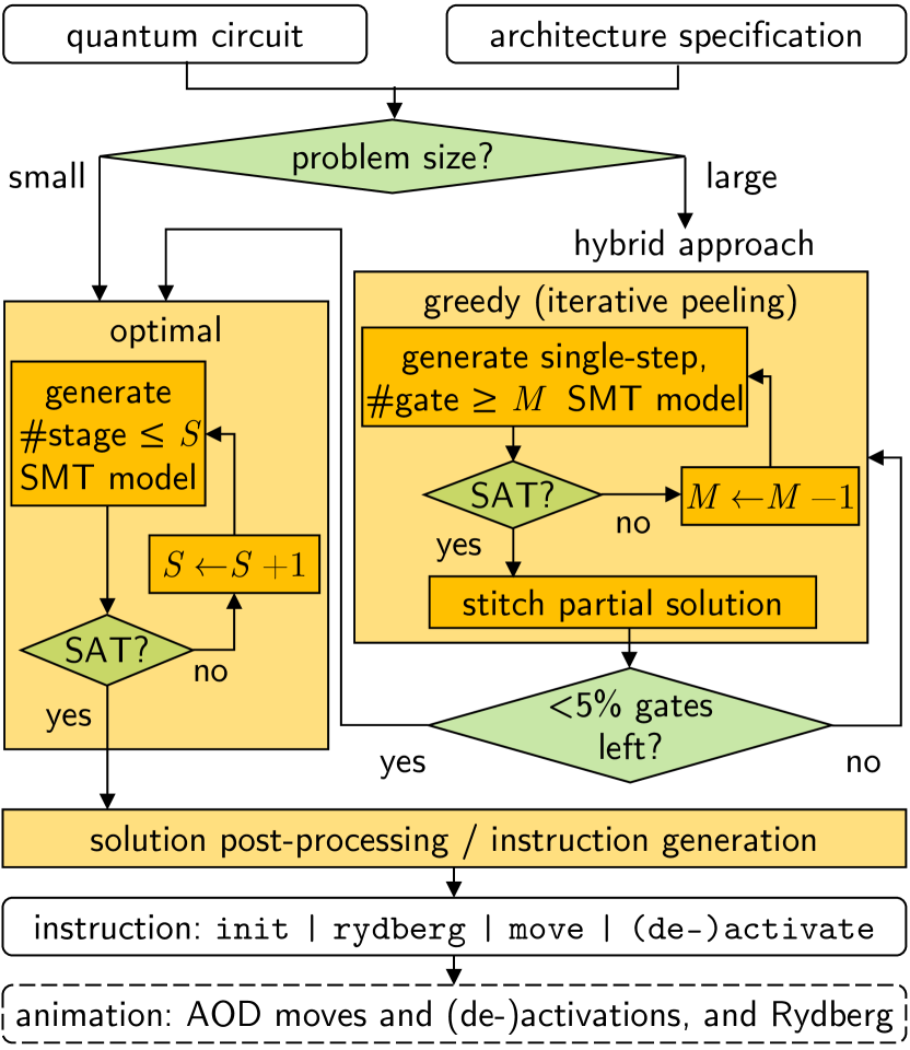
Figure 3: Workflow of our compiler OLSQ-DPQA. The inputs to the compiler are the quantum circuit to execute and the specifications of the DPQA architecture considered. If the problem is small, the compiler directly takes the optimal approach by constructing an SMT model where all the gates are applied to the first $S$ stages. If the model is satisfiable, then we find a solution; otherwise, we increase $S$ and try again. Thus, we find a solution with the minimum number of stages in the end, because lower-depth models are all checked and unsatisfiable. The SMT solution goes through a post-processing to extract the instructions for executing the quantum circuit on DPQA. There are only five types of instruction: init for initialization; rydberg to turn on the Rydberg laser and perform two-qubit gates; move for changing the coordinates of AOD rows/columns; activate for turning on certain AOD rows/columns for atom transfer; and deactivate for turning off certain AOD rows/columns. If the problem is large, the compiler takes a hybrid approach by iteratively “peeling off” the maximum number of gates possible. It generates a single-step (two-stage) SMT model with a constraint of executing more than $M$ gates in one step. After possible decreases of $M$, we find the solution with as many gates executed in one step as possible. Then, we stitch this partial solution, which is one “layer peeled off”, to the whole solution. When the problem becomes sufficiently small ($5\%$ of gates left), the compiler switches to the optimal approach.

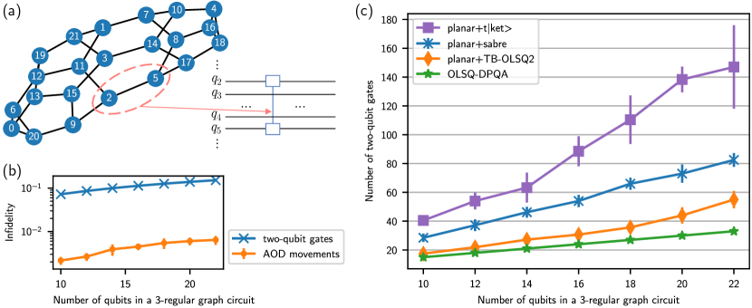
Figure 4: Evaluation of the optimal compiler. (a) Graph circuits. Given any graph, we treat each node as a qubit and add a two-qubit entangling gate for every edge in the graph to construct the graph circuit. We assume the gates are commutable, so gate order does not matter. The benchmarks used are graph circuits generated by 3-regular graphs of size 10 to 22. For each size, we have 10 random graphs. (b) Comparison of infidelity caused by the Rydberg laser (performing two-qubit gates) and the AOD movements. The latter is 27x smaller on average. We make such estimation using $99.5\%$ two-qubit gate fidelity [4] and a movement scheme that yields low atom heating as in Ref. [3]. (c) Comparison of the number of two-qubit gates required on a fixed planar architecture (Google’s Sycamore) and DPQA employing different compilers. Error bars are standard deviations among 10 random graphs of the same size. The compilers are t$|$ket$\rangle$, SABRE (integrated in Qiskit), and TB-OLSQ2. Note that TB-OLSQ2 is optimal for fixed architectures, but there is still a significant gap (1.7x) between it and the optimal DPQA compiler. The gaps mainly come from SWAP gates inserted on the fixed architecture, which requires three entangling gates (controlled $R_{z}$) [41].

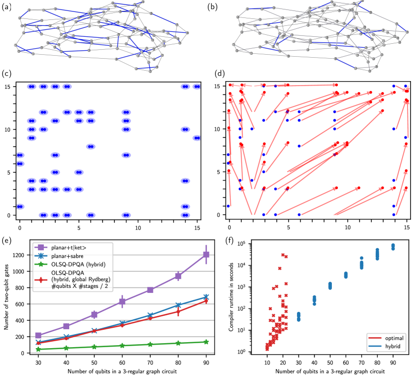
Figure 5: Evaluation of the greedy-optimal hybrid compiler. (a, b) One of the largest benchmarks we are able to compile, a 90-node 3-regular graph. The highlighted edges are gates executed at the stages in (c) and (d), respectively. (c) One stage of the compiled result. The dots are qubits in SLM. The ovals indicate two-qubit gates performed at this stage, which have a 1-to-1 correspondence with the edges in (a). After this stage, some qubits are transferred to AOD and moved. (d) The next stage. The red dots are the AOD qubits, and the arrows indicate the parallel movements from (c) to the current state. Readers are welcome to check out our code base for this animation. (e) Comparison of the number of two-qubit gates required on a fixed planar architecture (10x10 grid) using different compilers and DPQA. For DPQA, the number of two-qubit gates scales as $n$, whereas for the state-of-the-art heuristic solver on the fixed planar architecture, SABRE, scales as $n^{1.52\pm 0.02}$ where $n$ is the number of qubits. DPQA requires far less two-qubit gates, 5.1X less than SABRE, and scales linearly. (f) Comparison of runtime of the optimal and hybrid approaches in OLSQ-DPQA. Since both of them internally rely on SMT solving, the runtime scalings are both exponential in the size of the graph with which we generate the quantum circuit. However, the hybrid approach is significantly faster so that large instances can be solved (up to 90 qubits in $10^{5}$ $\sim$ a day). Compared to the optimal approach, the scaling of the hybrid approach is mainly related to size rather than the specific graph, which is demonstrated by the much smaller spread of data points at the each size.

4 Optimal Compilation with SMT

Given the variables above, we can express the DPQA constraints. The simplest constraints are the bounds for variables. As a part of the architecture specification, we restrict the region where qubits can be put and moved. Depending on our field of view and $r_{b}$, there are upper bounds $X$ and $Y$ of how many traps we have in horizontal and vertical directions. So, we have integer inequality constraints:

$$0\leq x_{i,s}<X,\ 0\leq y_{i,s}<Y\quad\forall i,s.$$ (1)

Depending on how many AOD columns and rows are at our disposal, we also restrict the range of $c_{i,s}$ and $r_{i,s}$ with constants $C$ and $R$. Other constraints may also require Boolean logic, e.g., the qubits in SLM are stationary between two stages:

$$\left(a_{i,s}=0\right)\Rightarrow\left(x_{i,s+1}=x_{i,s}\right)\wedge\left(y_{i,s+1}=y_{i,s}\right)\quad\forall i,s.$$ (2)

For example, $q_{4}$ is in SLM at stage 0, i.e., $a_{4,0}=0$, so its site indices remain the same between stage 0 and 1, i.e., $x_{4,1}=x_{4,0}$ and $y_{4,1}=y_{4,0}$. As it turns out, we can construct all the DPQA constraints with first-order logic and integer inequalities (Appendix D) which enables automatic reasoning of these constraints.

Satisfiability modulo theories (SMT) solvers are tools that can solve valid variable assignments given this form of constraint. We can encapsulate the variable definitions and constraints expressed with these variables in an SMT model. When provided with a model, an SMT solver can check whether it is satisfiable. If so, the solver returns the variable assignments which are all we need to execute circuits because our variables completely capture the architecture in spacetime. If the model is not satisfiable, some of our bounds are too small for valid variable assignments that will satisfy all the constraints.

With an SMT solver, we are able to not only solve valid assignments to compile circuits, but also guarantee the optimality of the solution with respect to some objective function, presented as the optimal branch in Fig. 3. So far, the dominating error source of DPQA is the Rydberg laser (see Appendix A.4 for detail), so we ignore the single-qubit gates for now and add them back after layout synthesis. Then, our objective is the number of times we turn on the Rydberg laser, i.e., the number of stages of parallel two-qubit gates, or, circuit depth $S$. Thus, we use relatively large spatial bounds ($X,Y,R,C$) which is more likely to yield satisfiable models with a lower $S$. We start by setting $S$ to a lower bound, e.g., the critical path in the circuit, which is 3 for the one in Fig. 2a. If the SMT solver returns unsatisfiable, we increase $S$ and invoke the solver again, until it finds a valid solution with $S_{\mathrm{opt}}$ stages. With this procedure, the optimality is guaranteed since we have checked for any smaller $S$ yield unsatisfiable models before finding the solution. If $S$ increases beyond the number of gates, we conclude that the spatial bounds are too small and increase them. The procedure will terminate since any finite circuit of size $P$ can be run in a finite spacetime volume bounded by $P\times P\times P$.

The variable assignments are not yet a DPQA executable. We need to post-process the SMT solution to produce DPQA instructions. For example, we must know the beginning and end coordinates of each AOD column, which are stored distributively in the $x_{i,s}$ and $c_{i,s}$ variables. In the example of Fig. 2, we find $q_{2}$ is in column $1$ and $x=1$ at stage 0, i.e., $c_{2,0}=1$ and $x_{2,0}=1$, and $x=2$ at stage 1, i.e., when $x_{2,1}=2$, we infer that the AOD column 1 travels from $x=1$ to $x=2$. As such, the information in the SMT solution will be translated to five types of basic DPQA instructions: init for initial qubit loading, rydberg for illuminating the Rydberg laser, move for AOD movements, activate for activating AOD rows/columns, and deactivate for deactivating AOD rows/columns. These instructions are readily executable on DPQA and our compiler can also generate animations from the instructions to view the execution process in action.

We benchmark the effectiveness of DPQA and our compiler, OLSQ-DPQA, on a set of quantum circuits constructed using random graphs, as illustrated in Fig. 4a. For a given graph, we assign each node to a qubit and apply a two-qubit gate for every edge. For simplicity, we consider problems where these gates are commutable, like the controlled-$R_{z}$ gates available on DPQA [40, 4], so the compiler also explores freedom of permuting gate ordering. By considering measured 1.5 s coherence times [3] and 99.5% CZ gate fidelity [4] in DPQA, as expected, we find the main error source is the Rydberg laser (Fig. 4a). The infidelity associated with AOD movements based on real experimental parameters (details in Appendices A and E), is revealed to be $\sim 27\times$ smaller than the infidelity of two-qubit gates, as shown in Fig. 4b, indicating that DPQA is promising for realizing highly nonlocal graphs where motion can be complex, and that increasing two-qubit gate fidelity is the main way to continue boosting fidelity.

We now compare our DPQA compilation results to the compilation results on fixed planar architectures, where instead of physically moving qubits around, qubits are moved around using two-qubit SWAP gates. As expected, DPQA combined with the optimal compiler requires significantly fewer two-qubit gates. We tested a few compilers that perform layout synthesis for the fixed architecture by inserting SWAP gates: t$|$ket$\rangle$ [42], a heuristic compiler used in leading QAOA experiments [43]; SABRE [17], a heuristic compiler integrated in leading quantum programming framework, Qiskit [44]; and TB-OLSQ2 [14], a leading optimal compiler for fixed architecture. The gaps of the number of two-qubit gates for a QAOA benchmark with 22 nodes in the graph are 4.5x, 2.5x, and 1.7x, respectively.

5 Hybrid Approach

The runtime for SMT solving scales exponentially in the worst case, so the optimal compiler can take a very long time to solve certain cases, as seen in Fig. 5f. Due to the complicated constraints, it is also challenging to design near-optimal purely heuristic algorithms to search the solution space of DPQA. Therefore, we adopt a two-level approach, as illustrated in the hybrid approach in Fig. 3. For large problems, at the higher level, we apply a greedy heuristic in that, at every stage, we find the AOD movement to maximize the number of gates to execute in the next stage and we repeat this process until there are a sufficiently small number of gates remaining. Then, we switch to the optimal approach. This technique is inspired by ‘iterative peeling’ for routing classical integrated circuits with multi-layer routing layers [45].

Specifically, if there are still gates to execute, we construct a “single-step” SMT model with two stages and set the qubit location of the initial stage to that of the current stage in the full solution. For instance, suppose the compiler has already processed $g_{0}$ to $g_{4}$ in Fig. 2a and progressed to stage 1 (Fig. 2c). In the single-step model, all initial locations are set by the previous partial solution, e.g., $x_{4,0}=1$ since $q_{4}$ at $x=1$ in Fig. 2c. Then, we optimize the number of gates executed in the second stage in the single-step model with a procedure similar to the one in the optimal approach, except that we decrease the number of gates to execute in the each stage from an upper bound of $M$ instead of increasing the number of stages from a lower bound. The upper bound is the maximum matching number of the graph constructed from the remaining gates. In our example, the remaining gates $g_{5}$ and $g_{7}$ both act on $q_{0}$, whereas $g_{6}$ and $g_{8}$ both act on $q_{1}$, so only one gate in each of these two pairs can be executed together, i.e., the maximum matching number is 2. The compiler appends the single-step model with a constraint that says there are at least 2 gates executed at the next stage and invokes the SMT solver, which can find such a solution (Fig. 2e). We stitch this partial solution to the full solution, remove gates $g_{5}$ and $g_{6}$ which is a layer of gates “peeled off”, and continue to the next “peeling”. If there are only a few gates remaining (we opt for $5\%$) the compiler switches to the optimal approach to solve for the final stages.

The hybrid approach cannot fundamentally improve the runtime scaling to polynomial because it still relies on SMT solving, but it greatly accelerates the process, with some sacrifice on optimality. As exhibited in Fig. 5f, it is much faster than the optimal compiler and the divergence of runtime within benchmarks of the same size is also much smaller. Within a reasonable amount of time ($10^{5}$s $\approx$ a day), the hybrid compiler managed to compile some 90-qubit circuits whereas the optimal compiler, in the worst case, can only compile up to the 22-qubit circuit. We present one of the largest circuits compiled in Fig. 5a-d: (a, b) exhibit the graph generating the quantum circuit which has a complex connectivity; (c, d) are two stages in the program execution. This hybrid approach is implemented in the OLSQ-DPQA compiler, which is open-source under the BSD 3-clause license. The code base includes Python scripts that 1) generate the SMT models and iteratively invoke an SMT solver, Z3 [46] to solve them, 2) generate DPQA instructions and animations based on SMT solutions, 3) draw plots in the evaluations. The dependencies are Python packages Z3 [46], PySAT [47], NetworkX [48], and Matplotlib [49]. The code base also includes all SMT solutions in the evaluations and some example animations.

We compare the required number of two-qubit gates by DPQA and a fixed planar architecture (10x10 grid) in Fig. 5e. We find that the savings from DPQA on such a large system is significant compared to the fixed architecture: 5.1x and 8.9x reduction in the number of two-qubit gates, respectively, compared to the compilation results by SABRE and t$|$ket$\rangle$. If the heuristics place qubits in an $\sqrt{n}$-by-$\sqrt{n}$ region, each gate may require $O(\sqrt{n})$ SWAPs to route. Then, for $O(n)$ gates, as in our benchmark set, $O(n^{1.5})$ SWAPs are required. We observe this scaling in the results of SABRE: with a log-log fitting, the number of two-qubit gates scales in the $1.52\pm 0.02$ power of the number of qubits. In comparison, DPQA routes the gates by AOD movements instead of SWAPs, so the number of gates scales linearly. This result assumes that DPQA is equipped with an individually addressable Rydberg laser (or other methods of turning off the Rydberg excitation locally) that does not accumulate the same error on idling qubits (e.g., in [50]).

6 Discussion and Outlook

In this work, we studied the constraints of existing dynamically field-programmable qubit arrays (DPQA) architecture regarding compilation and discretization of the architecture. Then, we developed a compiler for the architecture, OLSQ-DPQA. The compiler and results developed here are suited to a wide range of applications in neutral atom quantum computation. Broadly, combined with state-of-the-art neutral atom hardware and the ability of our compiler to output hardware-level instructions, these techniques would allow us to specify an arbitrary quantum circuit with arbitrary connectivity on approximately 100 qubits and then realize this circuit on quantum hardware. This can allow, for example, implementing circuits like the quantum fourier transform on significantly larger numbers of qubits than previously realized [51, 52], implementing nonlocally connected, high-rate quantum low-density parity check (LDPC) codes [53], or studying evolution in exotic Hamiltonians [54].

In particular, the results presented for realizing circuits on random 3-regular graphs on 90 qubits can directly be applied to various problems. For combinatorial optimization, one can utilize the class of graphs examined here to study the quantum algorithm performance on problems such as MAXCUT or MIS with either the Quantum Adiabatic Optimization Algorithm (QAOA) [55] or the trotterized adiabatic evolution [13]. Realizing such a complex evolution on nonlocally connected graphs such as in Fig. 5 can be used for efficient quantum supremacy and information scrambling experiments [56, 57]. In such an approach, one can choose to employ the first few, most efficient layers of the compilation to implement classes of random nonlocally connected graphs.

The compiler used here can be expanded further along multiple axes. Given the generality and flexibility of the framework, the compiler can adapt to new hardware features before implementation and inform hardware design for neutral atom quantum computers. We demonstrated a significant gate reduction showcasing the power of the reconfigurable quantum computing architectures. Such results incentivize further developments of DPQA hardware, e.g., scaling up DPQA to over 1000 qubits, including mid-circuit readout and quantum error correction, to execute large scale quantum circuits. To support hardware at such a scale, a high-performance efficient compilation is required, and our formulation provides a solid basis to start constructing such compilation methods. In addition, the comparison of results with local and global Rydberg laser control indicates the importance of hardware to have locally switchable Rydberg excitation [50] or “idle” zones [3]. Qubits can be stored in these zones to avoid accumulating errors when other qubits are being operated on. The idling zones also simplifies the compilation problem since the qubits in these zones do not need to be spatially separated to avoid Rydberg interaction, which may greatly accelerate the compilation.

Appendix A DPQA Architecture

In an atom array system, each individual qubit is a single atom trapped in an individual optical tweezer, which enables a deterministic control over the qubit position. The physics of atomic trapping, optical tweezers, and entangling gates leads to several key implications. These implications serve as the interface between physics and computer science with which we reason about the variables, constraints, and optimization procedure in our compilers. Thus, we enumerate them in this appendix for reference. For the specific technical parameters, we follow the state-of-the-art experimental work [4, 3].

A.1 Atom Trapping

One trap cannot hold more than one atom. Otherwise, the atoms may expel each other out of the trap.

Implication 1.

One trap can hold zero or one atom at any time during the computation.

Two orthogonal optical components generate AOD tweezers. The X component produces a horizontal pattern, and the Y component multiplies this pattern by a vertical pattern. In contrast, an arbitrary phase hologram on a spatial light modulator produces SLM tweezers. As a result, we can place each SLM tweezer in an arbitrary location. However, to enable massive parallelism of gate execution, the geometry of the SLM and the AOD should be similar.

Implication 2.

AOD and SLM optical trap arrays are rectangular arrays that extend in the X and Y direction in the 2D plane.

E.g., in Fig. 2b, the AOD is a rectangular array with two rows and four columns, indicated by the dashed grid. The dynamically programmable processor in [3] uses up to 24 qubits, but system sizes of 100s of qubits are attainable as was done in [13], and both SLM and AOD grids have been used in system sizes as large as 16x16 each [58].

Because of the finite optical resolution of the microscope generating tweezers, traps of the same array cannot be closer than a given minimum spacing. In [3], it is $2\upmu$m.

Implication 3.

There is a minimal separation between two rows or columns of traps in the same array, $d_{s}$.

A.2 Array Movements

AOD traps can move whereas SLM traps cannot. Thus, it may seem to some readers that SLM is strictly less general than AOD, rendering the notion of SLM redundant for compilation. However, an advantage of SLM is that we can turn off the unused traps based on the compilation result. As part of the architecture specification, we make a certain number of SLM traps available to the compiler, but some of them are never used throughout the compiled result. Then, we simply ignore them when we generate the SLM in the beginning of the experiment, which saves some laser power. Although total laser power is not a bottleneck at the moment, the savings of SLM is beneficial for future scaling-up. Thus, we keep SLM in the formulation instead of just treating it as a special case of AOD.

Implication 4.

If the array is the SLM type, the traps are stationary.

E.g., $q_{4}$ stays at the same place throughout Fig. 2b-2f.

The control we have on the AOD traps are the Y coordinate of each row and the X coordinate of each column.

Implication 5.

If the array is the AOD type, a row/column of traps move together.

E.g., from Fig. 2b to 2c, the AOD row of $q_{5}$, $q_{3}$, and $q_{1}$ moves upwards, and the column of $q_{2}$ and $q_{3}$ moves to the right.

Per Impl. 3, we cannot place two rows/columns too close together. If rows A and B move across each other, they must have been closer than the minimum spacing at some point, which is prohibited.

Implication 6.

If the array is the AOD type, a row cannot cross over another row, a column cannot move over another column.

In [3], the relation between movement time $t$ and travel distance $D$ is set as $t=T_{0}\sqrt{D/D_{0}}$ to maintain constant heating of the atoms during movements. We follow their setting $T_{0}=200\upmu$s and $D_{0}=110\upmu$m so that the heating is sufficiently low.

A.3 Quantum Gates

Single-qubit gates are high-fidelity operations that are generically easy to perform locally (see [40]).

Implication 7.

Arbitrary single-qubit gates can be addressed to each qubit individually.

We perform two-qubit operations with a specific type of laser to excite the atoms to Rydberg state. In this state, atoms within a certain distance will interact strongly and cannot be excited simultaneously. The characteristic distance of this interaction is the Rydberg blockade radius $r_{b}$ ($7.5\upmu$m in [3]). This blockade mechanism is the basis of two-qubit entangling gates; only if two atoms are within an $r_{b}$ of each other can they perform a two-qubit gate. The specific gate implemented in [3] is the Levine-Pichler CZ gate, which is a special case of controlled-$R_{z}$ gates available in DPQA [40].

Implication 8.

Two qubits $q$ and $q^{\prime}$ can only perform an entangling two-qubit gate when they are within a blockade radius, i.e., $|\vec{x}_{q}-\vec{x}_{q^{\prime}}|\leq r_{b}$, and they are both illuminated by the Rydberg laser.

The Rydberg laser is global in the sense that it illuminates all the qubits, as done in [13, 3]. When we turn on the laser, we cannot “switch off” the interaction of a pair if they are within range.

Implication 9.

If $q$ and $q^{\prime}$ are within $r_{b}$ and illuminated by the Rydberg laser, they will go through a two-qubit entangling gate.

If two atoms are sufficiently separated, $>2.5r_{b}$ in practice, they will not interact even if excited by the Rydberg laser. If there are more than two atoms that are not sufficiently separated, they go through a joint quantum process which is not a well-defined gate.

Implication 10.

For any three qubits $q_{0}$, $q_{1}$, and $q_{2}$, at most one of the following is true when the Rydberg laser is on: $|\vec{x}_{q_{0}}-\vec{x}_{q_{1}}|<2.5r_{b}$, $|\vec{x}_{q_{1}}-\vec{x}_{q_{2}}|<2.5r_{b}$, $|\vec{x}_{q_{2}}-\vec{x}_{q_{0}}|<2.5r_{b}$. That is, only disjoint pairs of qubits may entangle simultaneously.

A.4 Error Source

Errors can occur during the gates or the idling time (including AOD movements, activation, and deactivation). In the evaluation in this paper, the average idling time is only $2.6\%$ of the qubit lifetime (coherence time) in the largest benchmark (90-node QAOA). Thus, the idling time plays a relatively small role in the error source. In addition, the single-qubit operations are significantly higher fidelity ($99.99\%$) than the two-qubit entangling gates ($99.5\%$) [3, 4]. A global Rydberg laser for the two-qubit gates induces the same error rate on all qubits whether they are involved with a two-qubit gate at this stage or not.

Implication 11.

The main computational error source is the number of layers of two-qubit gates.

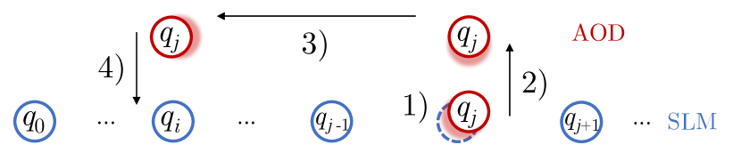
Figure 6: Universal QC with one AOD trap and one SLM row. Single-qubit gates executes directly. To implement an entangling gate on an arbitrary qubit pair: 1) pick $q_{j}$ from SLM to AOD, so the original SLM trap is empty (dashes), 2) move the AOD trap up, 3) adjust the AOD trap horizontally until $q_{i}$ and $q_{j}$ align, then 4) shift the AOD trap down to perform the gate.

A.5 Atom Transfer

So far, we have described atoms staying in their own individual tweezer traps, as was focused on in the experiments of [3]. However, it has previously been demonstrated that atoms can be transferred between tweezer traps [2] by reducing the intensity of one tweezer trap while increasing or maintaining the intensity of another tweezer trap. In the system considered here, in an AOD array, we can tune the individual intensity of AOD rows and columns to transfer to/from SLM traps: e.g., Fig. 2e, we turn off the leftmost AOD column so that $q_{5}$ is transferred to SLM.

A.6 Universality

With atom transfers, the architecture can perform universal quantum computing given a large enough area. Fig. 6 depicts a toy construction. We load the qubits to one SLM row with sufficient separations between the traps. There is one AOD trap working as delivery. Per Impl. 7, single-qubit gates are always executable. To apply an entangling gate on an arbitrary pair $(q_{i},q_{j})$, we perform the 4-step procedure illustrated in Fig. 6. Finally, we reverse the movements and put $q_{j}$ back to SLM. Now, we are ready for the next gate. With this construction, we can execute any single-qubit and two-qubit gate, so the architecture can perform universal QC. Of course, this construction is like the demonstration of the Turing machine in classical universal computing where efficiency is not considered. For example, we can easily put atoms in a square array that reduces the amount of time for movements.

Appendix B Quantum Layout Synthesis

The input of quantum layout synthesis consists of two parts: the coupling graph and the program/circuit to be executed. For instance, the coupling graph of Google’s Sycamore processor [5] is shown in Fig. 7a. In this graph, every node is a quantum register that can hold one qubit, and all possible two-qubit entangling operations/gates are represented by the edges. An example of a quantum program is exhibited in Fig. 7c, which is the quantum approximate optimization algorithm (QAOA) [59] applied to the Max-Cut problem of a 3-regular graph. The parameters $\gamma$’s and $\beta$’s are inputs from an outer layer classical optimization. The quantum program first initializes all qubits to state $|0\rangle+|1\rangle$ and iteratively applies the problem unitary $U_{C}(\gamma)$ and the driver unitary $U_{B}(\beta)$ for $p$ times, each iteration with different parameters $\gamma_{i}$ and $\beta_{i}$. $U_{B}$ consists of single-qubit $R_{x}$ gates on all qubits which can always be executed, so it is not challenging for the compiler. On the other hand, $U_{C}$, consisting of nine two-qubit ZZ-phase gates (Fig. 7b), is the center of attention in layout synthesis. These gates are induced by the 3-regular graph: for each edge in the graph, we apply a ZZ-phase gate to its two qubits.

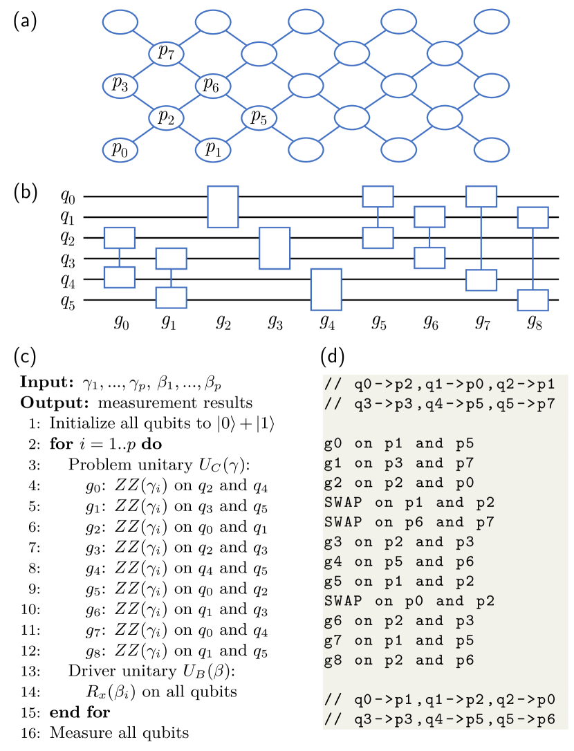
Figure 7: The quantum layout synthesis problem. (a) The (partial) coupling graph of Google Sycamore processor, as in [43]. The annotated quantum registers are made use of in this example. (b) Diagram of the quantum circuit to execute. (c) Pseudocode for QAOA applied to the Max-Cut problem. There are $p$ iterations of applying problem unitary $U_{C}$ and then driver unitary $U_{B}$. $U_{C}$ is implemented by the circuit in (b), though on different parameter $\gamma$ at different iterations. (d) A layout synthesis solution that runs circuit (b) on architecture (a). The comments are the initial and final qubit mappings.

For this example, we first need to map the qubits $q_{0}$ … $q_{5}$ to quantum registers, i.e., nodes in the coupling graph in Fig. 7a. E.g., on the top of the solution shown in Fig. 7d, $q_{2}$ is initially mapped to $p_{1}$ and $q_{4}$ is mapped to $p_{5}$. Since $p_{1}$ and $p_{5}$ are indeed adjacent in the coupling graph, the gate $g_{0}$ (on $q_{2}$ and $q_{4}$) can be executed. However, $g_{3}$ is on $q_{2}$ and $q_{3}$ that are mapped to nonadjacent registers $p_{1}$ and $p_{3}$. In this case, we need to insert a special gate named SWAP on $p_{1}$ and $p_{2}$ before $g_{3}$ that exchanges the two registers’ qubits. After the SWAP, $q_{2}$ maps to $p_{2}$ that is adjacent to $p_{3}$ which is holding $q_{3}$. Then, $g_{3}$ can be executed under this updated mapping.

Note that SWAP is not a native gate in most QC architectures. To achieve its effect, we need three native entangling gates and a few single-qubit gates, whether the native entangling gate is a CNOT gate or a Cross-Resonance gate on IBM processors [41], or a $\sqrt{i\mathrm{SWAP}}$ gate or a SYC gate on Sycamore [43]. Currently, the fidelity of entangling gates is low, so SWAPs are expensive. Thus, layout synthesis [14, 15, 16] is a very important, if not the most important, step in compilation as it determined the SWAPs to be inserted. It is also referred to as qubit mapping [17, 18, 19, 20, 21, 22, 23], qubit placement [24, 25, 26], or allocation [27, 28, 29]. Minimizing the number of SWAPs, or the number of gate layers in layout synthesis is proven to be NP-hard [24, 15, 27, 30]. Following the above approach, layout synthesis for DPQA is even more challenging because the coupling graph can change across different stages of the circuit execution, so we opt for a different formulation in this work.

DPQA is a relatively new technology, so previous works on compilation are for Rydberg atoms trapped in an SLM array that has fixed connectivity during the computation. There are both experimental [13] and theoretical/computational [60, 61] works exploring solving the Max-Independent-Set problem using adiabatic quantum algorithm on SLM arrays. Ref. [50] applies QAOA to the Max-Cut problem on an SLM array. In this case, the layout synthesis problem is as if for a fixed architecture, like described above. Ref. [31] discusses logic synthesis for hypothetical architectures that can perform a three-qubit gate pulse sequence, but leverages existing layout synthesis tools for fixed architectures. Ref. [32] also utilizes existing layout synthesis tools but features the ability to perform long-range Rydberg interaction. However, it requires a hypothetical architecture where the Rydberg range of qubits can be individually tuned.

The most relevant previous work is [33] on an atom array architecture that can perform ‘1D displacements’ during the computation, similar to only horizontal shifts of AOD rows. This ‘1D displacement’ is only a small subset of the AOD movements we support. It does not capture the highly flexible motion demonstrated in the recent experiments in [3], which future works will only continue to expand, whereas this work is able to capture the experimentally demonstrated techniques as well as future developments.

Appendix C Spatial Discretization of DPQA

There may be parallel executions of two-qubit entangling gates at different sites, so, per Impl. 10, the sites should be sufficiently separated to avoid unwanted Rydberg interactions. Also, to maximize usage, the tiling pattern of the sites should accord to the geometry of the tweezer arrays, which is a 2D grid per Impl. 2. The interaction sites are illustrated as shades in Fig. 8. In fact, our efforts in discretization is analogous to that of Mead and Conway [62] in VLSI chip design where an abstract basic length unit in semiconductor fabrication, $\lambda$, was introduced. The chip area is discretized to separated “lines” of $2\lambda$’s wide layout design. These dimensionless $\lambda$-rules helped the advancement of automated layout tools despite the fast developments in the fabrication technology that affects $\lambda$. Similarly, based on our discretization, our formulation holds even if the constants $r_{b}$, $2.5r_{b}$ and $d_{s}$ change. It is crucial to retain this flexibility for possible adjustments in physics experiments. E.g., we may want to excite the qubits to a higher Rydberg state, leading to a bigger $r_{b}$; or upgrading to higher-resolution microscope objective lenses, leading to a smaller $d_{s}$.

We allow several rows or columns to “stack” together at one interaction site to support gates between two AOD qubits. However, there is an upper bound on how many AOD rows/columns can be stacked together at a site because these AOD rows/columns cannot be too close to each other (Impl. 3). We denote the maximal stacking factor as $R_{\mathrm{STK}}$ and $C_{\mathrm{STK}}$, respectively. They are decided by the minimal AOD row/column separation $d_{s}$ and the Rydberg range $r_{b}$. The callout in Fig. 8 exhibits an extreme case where we need to entangle two qubits $q_{i}$ and $q_{j}$ at the corners of the site. This requires $[(R_{\mathrm{STK}}-1)^{2}+(C_{\mathrm{STK}}-1)^{2}]d_{s}^{2}\leq r_{b}^{2}$. $r_{b}=7.5\upmu$m and $d_{s}=2\upmu$m, $R_{\mathrm{STK}}=C_{\mathrm{STK}}=3$ satisfies the inequality.

In fact, the ticks on $x$ and $y$ axes in Fig. 1c and Fig. 2b-f indicates the interaction sites. At each stage, per Impl. 10, there can be at most two qubits. Thus, there are five possible situations at a site: 1) empty, e.g., (0,1) at stage 0 (Fig. 2b); 2) one SLM qubit, e.g., (1,1) at stage 2 holds only $q_{4}$; 3) one AOD qubit, e.g., (3,1) at stage 0 holds only $q_{0}$; 4) one SLM qubit and one AOD qubit, e.g, (1,1) at stage 0 holds $q_{4}$ and $q_{2}$; 5) two AOD qubits, e.g., (1,0) at stage 0 holds $q_{5}$ and $q_{3}$.

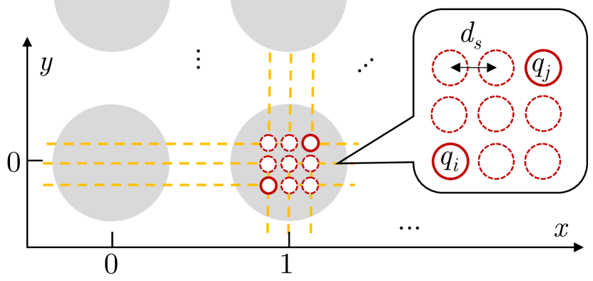
Figure 8: Discretization of space into interaction sites. The unit of X and Y is a sufficient distance to prevent Rydberg interaction. Interaction sites, indicated by shades, are centered at integer points on the 2D plane. A limited number of AOD rows or columns can stack together at one site. The callout is zooming into a site with three AOD rows and three columns.

The discretized coordinates (of interactions sites) are enough to specify AOD and SLM qubit locations, but they are not sufficient as the state of the architecture because of the stacking of rows/columns we just mentioned. For example, at stage 1 (Fig. 2c), both AOD rows are at $y=1$. Because of Impl. 6, the upper row cannot move across the lower row, e.g., $q_{2}$ cannot move below $q_{3}$. With only coordinates, it is hard to enforce constraints like this. Thus, as part of the architecture state, we also need to specify which row and column each AOD qubit is in. Finally, we have to specify whether the qubit is in SLM or AOD at each stage to handle atom transfers.

In conclusion, the computation progresses in multiple stages: stage 0, AOD movement 0, stage 1, AOD movement 1, stage 2, … At each stage, the architecture has a state consisting of interaction site indices (specifying location), AOD row/column indices, and an array index (specifying whether in SLM or AOD) for each qubit. During the AOD movement, the AOD row/column indices and the array index are invariant, but the site indices can change as AOD traps move in space.

Appendix D SMT Constraints

Constraints in this subsection come from physics implications on the architecture (circuit-independent), or fundamental properties of quantum programs (circuit-dependent). Let us use $N$ for the number of qubits and $G$ for the number of gates. Note that in the constraints below, we use ‘$=$’ to denote the operation that returns Boolean true if the l.h.s equals the r.h.s, and returns false otherwise. ‘$[A,B)$’ means from $A$ to $B-1$. All the concrete examples are taken from Fig. 2.

D.1 Circuit-Independent Constraints

Upper bounding the variables: $\forall i\in[0,N),s\in[0,S)$

$$0\leq x_{i,s}<X,$$ (3)

similarly for $y$, $c$, and $r$ with bounds $Y$, $C$, and $R$.

Stationary SLM enforces Impl. 4: $\forall i\in[0,N),\ \forall s\in[0,S-1)$

$$(a_{i,s}=0)\Rightarrow((x_{i,s+1}=x_{i,s})\wedge(y_{i,s+1}=y_{i,s})).$$ (4)

E.g., $q_{4}$ is in SLM at stage 0, i.e., $a_{4,0}=0$, so its site indices remain the same between stage 0 and 1, i.e., $x_{4,1}=x_{4,0}$ and $y_{4,1}=y_{4,0}$.

AOD moves by whole rows/columns enforcing Impl. 5: $\forall i\in[0,N),\ \forall s\in[0,S-1)$

$$(a_{i,s}=1)\Rightarrow((c_{i,s+1}=c_{i,s})\wedge(r_{i,s+1}=r_{i,s})).$$ (5)

E.g., $q_{5}$ is at column 0 at stage 0, $a_{5,0}=1$, so when it arrives at stage 1, the row/column index remains the same, i.e., $c_{5,1}=c_{5,0}$ and $r_{5,1}=r_{5,0}$, despite the changing site indices, i.e., $y_{5,1}\neq y_{5,0}$.

Site order implying row/column order enforcing Impl. 6 in the case of non-stacking rows/columns: $\forall i,i^{\prime}\in[0,N),\ \forall s\in[0,S)$

$$\begin{split}(x_{i,s}<x_{i^{\prime},s})&\Rightarrow\ (c_{i,s}<c_{i^{\prime},s}),\\ (y_{i,s}<y_{i^{\prime},s})&\Rightarrow(r_{i,s}<r_{i^{\prime},s}).\end{split}$$ (6)

E.g., at stage 0, $q_{5}$ is at $x=1$ while $q_{1}$ is at $x=2$, so $c_{5,0}<c_{1,0}$.

No crossing between AOD row/columns enforces Impl. 6 in the case of stacked rows/columns: $\forall i,i^{\prime}\in[0,N),\ \forall s\in[0,S-1)$

$$\begin{split}((a_{i,s}=1)\wedge(a_{i^{\prime},s}=1)\wedge&(c_{i,s}<c_{i^{\prime},s}))\\ &\Rightarrow(x_{i,s+1}\leq x_{i^{\prime},s+1}),\\ ((a_{i,s}=1)\wedge(a_{i^{\prime},s}=1)\wedge&(r_{i,s}<r_{i^{\prime},s}))\\ &\Rightarrow(y_{i,s+1}\leq y_{i^{\prime},s+1}).\\ \end{split}$$ (7)

E.g., at stage 0, $q_{1}$ is at row 0 and $q_{0}$ is at row 1, so $r_{1,0}<r_{0,0}$; at stage 1, $q_{1}$ and $q_{0}$ are both at $y=1$, which satisfies $y_{1,1}\leq y_{0,1}$.

Maximal stacking as in Appendix C: $\forall i,i^{\prime}\in[0,N),\ \forall s\in[0,S)$

$$\begin{split}((a_{i,s-1}&=1)\wedge(a_{i^{\prime},s-1}=1)\wedge\\ &(c_{i,s-1}-c_{i^{\prime},s-1}\geq C_{\mathrm{STK}}))\Rightarrow(x_{i,s}>x_{i^{\prime},s}),\\ ((a_{i,s-1}&=1)\wedge(a_{i^{\prime},s-1}=1)\wedge\\ &(r_{i,s-1}-r_{i^{\prime},s-1}\geq R_{\mathrm{STK}}))\Rightarrow(y_{i,s}>y_{i^{\prime},s}).\end{split}$$ (8)

(When $s=0$, the $s-1$ above is 0; otherwise, it is $s-1$.) E.g., at stage 0, $q_{5}$ is in column 0 while $q_{0}$ is in column 3, $c_{0,0}-c_{5,0}=3\geq C_{\mathrm{STK}}$, so $x_{0,1}>x_{5,1}$, i.e., they cannot be at the same site at stage 1.

One atom, one trap. There cannot be two atoms in one trap, thus imposing Impl. 1 and 10. If both atoms are in AOD, either their row or column index is different; if both are in SLM, either their site $x$ or $y$ index is different: $\forall i\in[0,N),\ \forall i^{\prime}\in[i+1,N),\ \forall s\in[0,S)$

$$\begin{split}((a_{i,s}=1)&\wedge(a_{i^{\prime},s}=1)\\ &\Rightarrow((c_{i,s}\neq c_{i^{\prime},s}))\vee((r_{i,s}\neq r_{i^{\prime},s})),\\ ((a_{i,s}=0)&\wedge(a_{i^{\prime},s}=0)\\ &\Rightarrow((x_{i,s}\neq x_{i^{\prime},s}))\vee((y_{i,s}\neq y_{i^{\prime},s})).\end{split}$$ (9)

(Optional) No atom transfer by fixing array index (which is what we do in the evaluations for the optimal compiler): $\forall i\in[0,N),\ \forall s\in[0,S)$

$$a_{i,s}=a_{i,0}.$$ (10)

If it is allowed for an atom to transfer to an empty trap at a same site, i.e., forbidding transfer when there are two atoms at a site, $\forall i\in[0,N),\ \forall i^{\prime}\in[i+1,N),\ \forall s\in[0,S-1)$

$$\begin{split}((x_{i,s+1}=&x_{i^{\prime},s+1})\wedge(y_{i,s+1}=y_{i^{\prime},s+1}))\\ &\Rightarrow((a_{i,s+1}=a_{i,s})\wedge(a_{i^{\prime},s+1}=a_{i^{\prime},s})).\end{split}$$ (11)

D.2 Circuit-Dependent Constraints

Gate collision. If two gates act on the same qubit, they cannot be executed at the same stage, e.g., $g_{0}$ and $g_{3}$ both act on $q_{2}$, so $t_{0}\neq t_{3}$.

Gate dependence. If the order of execution between two gates cannot be changed, we ensure this by $t_{j}<t_{j^{\prime}}$ if $g_{j^{\prime}}$ depends on $g_{j}$.

Connectivity ensures Impl. 8. Two qubits should be at the same site in order for an entangling gate to execute: $\forall j\in[0,G),$ $g_{j}$ acting on $q_{i}$ and $q_{i^{\prime}}$, $\forall s\in[0,S)$

$$(t_{j}=s)\Rightarrow\ ((x_{i,s}=x_{i^{\prime},s})\wedge(y_{i,s}=y_{i^{\prime},s})).$$ (12)

E.g., $g_{0}$ at stage 0 is on $q_{2}$ and $q_{4}$, so $x_{2,0}=x_{4,0}$ and $y_{2,0}=y_{4,0}$.

Interaction exactness enforces Impl. 9. We pre-compute a list $\rho_{i,i^{\prime}}$ for each pair of qubits ($q_{i}$ and $q_{i^{\prime}}$) that contains all the $j$ if $g_{j}$ acting on them. In the example of Fig. 2, there is only one gate $g_{2}$ acting on $q_{0}$ and $q_{1}$, so $\rho_{0,1}=\{2\}$; in contrast, there is no gates on $q_{0}$ and $q_{8}$, so $\rho_{0,8}=\emptyset$. If $\rho_{i,i^{\prime}}\neq\emptyset$, then two qubits must be at the same site at some stage, and one of the gates on them is being executed at this stage: $\forall i\in[0,N),\ \forall i^{\prime}\in[i+1,N),\ \mathrm{s.t.}\ \rho_{i,i^{\prime}}\neq\emptyset,\ \forall s\in[0,S)$

$$((x_{i,s}=x_{i^{\prime},s})\wedge(y_{i,s}=y_{i^{\prime},s}))\Rightarrow\left(\bigvee_{j\in\rho_{i,i^{\prime}}}t_{j}=s\right).$$ (13)

Conversely, if $\rho_{i,i^{\prime}}=\emptyset$, the qubits should not be at the same site ever: $\forall i\in[0,N),\ \forall i^{\prime}\in[i+1,N),\ \mathrm{s.t.}\ \rho(i,i^{\prime})=\emptyset,\ \forall s\in[0,S)$

$$(x_{i,s}\neq x_{i^{\prime},s})\vee(y_{i,s}\neq y_{i^{\prime},s}).$$ (14)

D.3 Enforcing Cardinality

There are two ways to enforce cardinality: implicitly in variable definition or explicitly with a cardinality constraint. The implicit approach is mainly for dimensions involved in the definition of the variables in the SMT model. Our arrays of variables have two dimensions: the qubit and the stage, which means whatever the model can possibly express is a computation using that many qubits and that many stages. The number of stages, $S$, in the optimal compiler is bounded in this approach: we only construct variables for $S$ stages. If $S$ is too small to execute the whole circuit, the model is unsatisfiable, so we need to add more variables. When the model becomes satisfiable, we have not introduced more variables than needed. Considering the exponential scaling of SMT solving to model size, we opt for the implicit approach to force the cardinality of stages.

An example of the explicit approach appends the SMT model with a constraint like

$$\sum_{j\in[0,G),s\in[S_{\text{LB}},S_{\text{UB}})}\mathrm{ITE}(t_{j}=s,\ 1,\ 0)\geq M,$$ (15)

where the stages between $S_{\text{LB}}$ and $S_{\text{UB}})$ are considered, and $\textrm{ITE}(\phi,w,z)$ means if the Boolean expression $\phi$ evaluates to true, return value $w$, otherwise $z$. Essentially, the l.h.s. is counting occurrences of a qubit pair appearing at the the same site at the same stage. If this sum is larger than $M$, then at least $M$ gates are executed between between stages $S_{\text{LB}}$ and $S_{\text{LB}}$. There are many ways to decompose the above equation to Boolean logic. We utilize the sequential counter approach offered by PySAT [47] in the hybrid method (Fig. 3). As a result, there are some intermediate Boolean variables introduced in the SMT model that do not correspond to any configurations of DPQA, purely for the sake of the cardinality constraint.

D.4 Scalability of the Model

The total number of variables in the optimal approach is $5NS+G$ where $N$ is the number of qubits, $S$ is the number of stages, and $G$ is the number of gates. The total number of constraints is $O(G^{2}+GS+N^{2}S)$. However, some of the variables have larger bounds. If we represent the integer variables by bit-vectors, the total number of bits to represent the variables is $NS\log(2XYRC)+G\log(S)$, where $X$ and $Y$ are the dimensions of the interaction site grid, $C$ and $R$ are the number of AOD columns and rows. The worst-case runtime of SMT solving is exponential, i.e., $O((N_{\mathrm{SLM}}N_{\mathrm{AOD}})^{NS}\cdot S^{G})$ where $N_{\mathrm{SLM}}=XY$ is the total number of SLM traps, and $N_{\mathrm{AOD}}$ is the total number of AOD traps. In the shallow circuit regime where $S$ can be seen as a constant, and if the program is induced by sparse graphs so that $G=O(N)$, the number of bits required is $O(N\log(N_{\mathrm{SLM}}N_{\mathrm{AOD}}))$ and the number of constraints is $O(N^{2})$. For each ‘peeling’ in the hybrid compiler, $S=2$.

Appendix E Evaluation Settings and Details

All the evaluation scripts are implemented in Python. We used the following packages: pytket 1.13.2 which is the Python interface of the compiler t$|$ket$\rangle$ [42]; and qiskit 0.42.1 which is the Qiskit [44] release containing the compiler SABRE (originated from [17]). Our compilers rely on a few Python packages. The versions used during the evaluations are: z3-solver 4.12.1.0 which is the Z3 SMT solver (originated from [46]); networkx 3.0 to calculate the maximum matching number of graphs; python-sat 0.1.8.dev1 to generate cardinality constraints; and matplotlib 3.6.2 to generate the figures. We ran the scripts on a desktop computer with an Intel Core i7-10700KF CPU and 32 GB RAM.

In our compilers, we set the spatial bounds to $X=Y=R=C=16$. For fairness of comparison, we assume the fixed architecture we are comparing with is equipped with the same gate set of DPQA. The SWAP gate requires three two-qubit entangling gates and six single-qubit gates. The benchmarks are graph circuits with 10, 12, 14, 16, 18, 20, 22, 30, 40, 50, 60, 70, 80, and 90 qubits. We generated 10 3-regular graphs of each size. For each graph, we assign a qubit to each node and append a two-qubit entangling gate for each pair of qubits connected by an edge to construct the graph circuit. We set the time limit to $10^{5}$ seconds which is approximately a day. Note that the compiler runtime can vary depending on the specific hardware and environment where it is run. The timeout instances are $20_{5}$, $22_{5}$, and $22_{8}$ for the optimal approach, $80_{1}$, $90_{0}$, $90_{2}$, $90_{6}$, $90_{8}$, and $90_{9}$ for the hybrid approach, where the subscripts are the indices of the graph. All the random graphs used are provided in the code base.

References

- [1] B. Tan, D. Bluvstein, M. D. Lukin, and J. Cong. “Qubit mapping for reconfigurable atom arrays”. In Proceedings of the 41th IEEE/ACM International Conference on Computer-Aided Design (ICCAD). San Diego, California (2022). Association for Computing Machinery.
- [2] J. Beugnon, C. Tuchendler, H. Marion, A. Gaëtan, Y. Miroshnychenko, Y. R. P. Sortais, A. M. Lance, M. P. A. Jones, G. Messin, A. Browaeys, and P. Grangier. “Two-dimensional transport and transfer of a single atomic qubit in optical tweezers”. Nature Physics 3, 696–699 (2007).
- [3] D. Bluvstein, H. Levine, G. Semeghini, T. T. Wang, S. Ebadi, M. Kalinowski, A. Keesling, N. Maskara, H. Pichler, M. Greiner, V. Vuletić, and M. D. Lukin. “A quantum processor based on coherent transport of entangled atom arrays”. Nature 604, 451–456 (2022).
- [4] S. J. Evered, D. Bluvstein, M. Kalinowski, S. Ebadi, T. Manovitz, H. Zhou, S. H. Li, A. A. Geim, T. T. Wang, N. Maskara, H. Levine, G. Semeghini, M. Greiner, V. Vuletic, and M. D. Lukin. “High-fidelity parallel entangling gates on a neutral atom quantum computer” (2023). arXiv:2304.05420.
- [5] Google Quantum AI. “Quantum computer datasheet”. url: https://quantumai.google/hardware/datasheet/weber.pdf.
- [6] IBM. “IBM quantum processor”. url: https://quantum-computing.ibm.com/services/docs/services/manage/systems/processors.
- [7] Rigetti. “Scalable quantum systems built from the chip up to power practical applications”. url: https://www.rigetti.com/what-we-build.
- [8] C. Chamberland, G. Zhu, T. J. Yoder, J. B. Hertzberg, and A. W. Cross. “Topological and subsystem codes on low-degree graphs with flag qubits”. Physical Review X 10, 011022 (2020).
- [9] Quantinuum. “Quantinuum H1, powered by Honeywell”. url: https://www.quantinuum.com/products/h1.
- [10] IonQ. “IonQ technology”. url: https://ionq.com/teczhnology.
- [11] D. Kielpinski, C. Monroe, and D. J. Wineland. “Architecture for a large-scale ion-trap quantum computer”. Nature 417, 709–711 (2002).
- [12] J. M. Pino, J. M. Dreiling, C. Figgatt, J. P. Gaebler, S. A. Moses, M. Allman, C. Baldwin, M. Foss-Feig, D. Hayes, K. Mayer, et al. “Demonstration of the trapped-ion quantum CCD computer architecture”. Nature 592, 209–213 (2021).
- [13] S. Ebadi, A. Keesling, M. Cain, T. T. Wang, H. Levine, D. Bluvstein, G. Semeghini, A. Omran, J.-G. Liu, R. Samajdar, X.-Z. Luo, B. Nash, X. Gao, B. Barak, E. Farhi, S. Sachdev, N. Gemelke, L. Zhou, S. Choi, H. Pichler, S.-T. Wang, M. Greiner, V. Vuletic, and M. D. Lukin. “Quantum optimization of maximum independent set using Rydberg atom arrays”. Science 376, 1209–1215 (2022).
- [14] W.-H. Lin, J. Kimko, B. Tan, N. Bjørner, and J. Cong. “Scalable optimal layout synthesis for NISQ quantum processors”. In Design Automation Conference (DAC). (2023).
- [15] B. Tan and J. Cong. “Optimality study of existing quantum computing layout synthesis tools”. IEEE Transactions on Computers 70, 1363–1373 (2021).
- [16] B. Tan and J. Cong. “Optimal layout synthesis for quantum computing”. In Proceedings of the 39th IEEE/ACM International Conference on Computer-Aided Design (ICCAD). Virtual Event, USA (2020). Association for Computing Machinery.
- [17] G. Li, Y. Ding, and Y. Xie. “Tackling the qubit mapping problem for NISQ-era quantum devices”. In Proceedings of the 24th International Conference on Architectural Support for Programming Languages and Operating Systems (ASPLOS). Providence, RI, USA (2019). ACM Press.
- [18] A. Zulehner and R. Wille. “Compiling SU(4) quantum circuits to IBM QX architectures”. In Proceedings of the 24th Asia and South Pacific Design Automation Conference (ASP-DAC). Tokyo, Japan (2019). ACM Press.
- [19] R. Wille, L. Burgholzer, and A. Zulehner. “Mapping quantum circuits to IBM QX architectures using the minimal number of SWAP and H operations”. In Proceedings of the 56th Annual Design Automation Conference 2019 (DAC). Las Vegas, NV, USA (2019). ACM Press.
- [20] D. Bhattacharjee, A. A. Saki, M. Alam, A. Chattopadhyay, and S. Ghosh. “MUQUT: Multi-constraint quantum circuit mapping on NISQ computers: Invited paper”. In Proceedings of the 38th IEEE/ACM International Conference on Computer-Aided Design (ICCAD). Westminster, CO, USA (2019). IEEE.
- [21] P. Murali, N. M. Linke, M. Martonosi, A. J. Abhari, N. H. Nguyen, and C. H. Alderete. “Full-stack, real-system quantum computer studies: Architectural comparisons and design insights”. In Proceedings of the 46th International Symposium on Computer Architecture (ISCA). Phoenix, Arizona (2019). ACM Press.
- [22] C. Zhang, A. B. Hayes, L. Qiu, Y. Jin, Y. Chen, and E. Z. Zhang. “Time-optimal qubit mapping”. In Proceedings of the 26th ACM International Conference on Architectural Support for Programming Languages and Operating Systems (ASPLOS). Virtual USA (2021). ACM.
- [23] B. Tan and J. Cong. “Optimal qubit mapping with simultaneous gate absorption”. In Proceedings of the 40th IEEE/ACM International Conference on Computer-Aided Design (ICCAD). Munich, Germany (2021). Association for Computing Machinery.
- [24] D. Maslov, S. M. Falconer, and M. Mosca. “Quantum circuit placement”. IEEE Transactions on Computer-Aided Design of Integrated Circuits and Systems 27, 752–763 (2008).
- [25] A. Shafaei, M. Saeedi, and M. Pedram. “Qubit placement to minimize communication overhead in 2D quantum architectures”. In Proceedings of the 19th Asia and South Pacific Design Automation Conference (ASP-DAC). Singapore (2014). IEEE.
- [26] D. Bhattacharjee and A. Chattopadhyay. “Depth-optimal quantum circuit placement for arbitrary topologies” (2017). arXiv:1703.08540.
- [27] M. Y. Siraichi, V. F. dos Santos, S. Collange, and F. M. Q. Pereira. “Qubit allocation”. In Proceedings of the 16th International Symposium on Code Generation and Optimization (CGO). Vienna, Austria (2018). ACM Press.
- [28] A. Ash-Saki, M. Alam, and S. Ghosh. “QURE: Qubit re-allocation in noisy intermediate-scale quantum computers”. In Proceedings of the 56th Annual Design Automation Conference (DAC). Las Vegas, NV, USA (2019). ACM Press.
- [29] M. Alam, A. Ash-Saki, and S. Ghosh. “An efficient circuit compilation flow for quantum approximate optimization algorithm”. In Proceedings of the 57th ACM/IEEE Design Automation Conference (DAC). San Francisco, CA, USA (2020). IEEE.
- [30] A. Botea, A. Kishimoto, and R. Marinescu. “On the complexity of quantum circuit compilation”. In Proceedings of the 11th Annual Symposium on Combinatorial Search. Stockholm, Sweden (2018). AAAI Press.
- [31] T. Patel, D. Silver, and D. Tiwari. “Geyser: A compilation framework for quantum computing with neutral atoms”. In Proceedings of the 49th Annual International Symposium on Computer Architecture (ISCA). New York, NY, USA (2022). Association for Computing Machinery.
- [32] J. M. Baker, A. Litteken, C. Duckering, et al. “Exploiting long-distance interactions and tolerating atom loss in neutral atom quantum architectures”. In Proceedings of the 48th Annual International Symposium on Computer Architecture (ISCA). Virtual Event (2021). IEEE Press.
- [33] S. Brandhofer, H. P. Büchler, and I. Polian. “Optimal mapping for near-term quantum architectures based on Rydberg atoms”. In Proceedings of the 40th IEEE/ACM International Conference on Computer-Aided Design (ICCAD). Munich, Germany (2021). Association for Computing Machinery.
- [34] A. Browaeys, D. Barredo, and T. Lahaye. “Experimental investigations of dipole–dipole interactions between a few Rydberg atoms”. Journal of Physics B: Atomic, Molecular and Optical Physics 49, 152001 (2016).
- [35] D. Barredo, S. de Léséleuc, V. Lienhard, T. Lahaye, and A. Browaeys. “An atom-by-atom assembler of defect-free arbitrary two-dimensional atomic arrays”. Science 354, 1021–1023 (2016).
- [36] H. Labuhn, D. Barredo, S. Ravets, S. de Léséleuc, T. Macrì, T. Lahaye, and A. Browaeys. “Tunable two-dimensional arrays of single Rydberg atoms for realizing quantum Ising models”. Nature 534, 667–670 (2016).
- [37] P. Scholl, M. Schuler, H. J. Williams, A. A. Eberharter, D. Barredo, K.-N. Schymik, V. Lienhard, L.-P. Henry, T. C. Lang, T. Lahaye, A. M. Läuchli, and A. Browaeys. “Quantum simulation of 2D antiferromagnets with hundreds of Rydberg atoms”. Nature 595, 233 – 238 (2021).
- [38] S. Ebadi, T. T. Wang, H. Levine, A. Keesling, G. Semeghini, A. Omran, D. Bluvstein, R. Samajdar, H. Pichler, W. W. Ho, S. Choi, S. Sachdev, M. Greiner, V. Vuletić, and M. D. Lukin. “Quantum phases of matter on a 256-atom programmable quantum simulator”. Nature 595, 227–232 (2021).
- [39] E. Urban, T. A. Johnson, T. Henage, L. Isenhower, D. D. Yavuz, T. G. Walker, and M. Saffman. “Observation of Rydberg blockade between two atoms”. Nature Physics 5, 110–114 (2008).
- [40] H. Levine, A. Keesling, G. Semeghini, A. Omran, T. T. Wang, S. Ebadi, H. Bernien, M. Greiner, V. Vuletić, H. Pichler, and M. D. Lukin. “Parallel implementation of high-fidelity multi-qubit gates with neutral atoms”. Physical Review Letters 123, 170503 (2019).
- [41] P. Gokhale, A. Javadi-Abhari, N. Earnest, Y. Shi, and F. T. Chong. “Optimized quantum compilation for near-term algorithms with OpenPulse”. In Proceedings of the 53rd Annual IEEE/ACM International Symposium on Microarchitecture (MICRO). Athens, Greece (2020). IEEE.
- [42] S. Sivarajah, S. Dilkes, A. Cowtan, W. Simmons, A. Edgington, and R. Duncan. “tket: A retargetable compiler for NISQ devices”. Quantum Science and Technology 6, 014003 (2020).
- [43] M. P. Harrigan, K. J. Sung, M. Neeley, K. J. Satzinger, F. Arute, K. Arya, J. Atalaya, J. C. Bardin, R. Barends, S. Boixo, M. Broughton, B. B. Buckley, D. A. Buell, B. Burkett, N. Bushnell, Y. Chen, Z. Chen, Ben Chiaro, R. Collins, W. Courtney, S. Demura, A. Dunsworth, D. Eppens, A. Fowler, B. Foxen, C. Gidney, M. Giustina, R. Graff, S. Habegger, A. Ho, S. Hong, T. Huang, L. B. Ioffe, S. V. Isakov, E. Jeffrey, Z. Jiang, C. Jones, D. Kafri, K. Kechedzhi, J. Kelly, S. Kim, P. V. Klimov, A. N. Korotkov, F. Kostritsa, D. Landhuis, P. Laptev, M. Lindmark, M. Leib, O. Martin, J. M. Martinis, J. R. McClean, M. McEwen, A. Megrant, X. Mi, M. Mohseni, W. Mruczkiewicz, J. Mutus, O. Naaman, C. Neill, F. Neukart, M. Y. Niu, T. E. O’Brien, B. O’Gorman, E. Ostby, A. Petukhov, H. Putterman, C. Quintana, P. Roushan, N. C. Rubin, D. Sank, A. Skolik, V. Smelyanskiy, D. Strain, M. Streif, M. Szalay, A. Vainsencher, T. White, Z. J. Yao, P. Yeh, A. Zalcman, L. Zhou, H. Neven, D. Bacon, E. Lucero, E. Farhi, and R. Babbush. “Quantum approximate optimization of non-planar graph problems on a planar superconducting processor”. Nature Physics 17, 332–336 (2021).
- [44] Qiskit contributors. “Qiskit: An open-source framework for quantum computing” (2023).
- [45] J. Cong, M. Hossain, and N. Sherwani. “A provably good multilayer topological planar routing algorithm in IC layout designs”. IEEE Transactions on Computer-Aided Design of Integrated Circuits and Systems 12, 70–78 (1993).
- [46] L. de Moura and N. Bjørner. “Z3: An efficient SMT solver”. In C. R. Ramakrishnan and J. Rehof, editors, Tools and Algorithms for the Construction and Analysis of Systems. Berlin, Heidelberg (2008). Springer.
- [47] A. Ignatiev, A. Morgado, and J. Marques-Silva. “PySAT: A Python toolkit for prototyping with SAT oracles”. In SAT. (2018).
- [48] A. Hagberg, P. Swart, and D. S Chult. “Exploring network structure, dynamics, and function using NetworkX”. Technical report. Los Alamos National Lab.(LANL), Los Alamos, NM (United States) (2008).
- [49] J. D. Hunter. “Matplotlib: A 2D graphics environment”. Computing in Science & Engineering 9, 90–95 (2007).
- [50] T. M. Graham, Y. Song, J. Scott, C. Poole, L. Phuttitarn, K. Jooya, P. Eichler, X. Jiang, A. Marra, B. Grinkemeyer, M. Kwon, M. Ebert, J. Cherek, M. T. Lichtman, M. Gillette, J. Gilbert, D. Bowman, T. Ballance, C. Campbell, E. D. Dahl, O. Crawford, N. S. Blunt, B. Rogers, T. Noel, and M. Saffman. “Multi-qubit entanglement and algorithms on a neutral-atom quantum computer”. Nature 604, 457–462 (2022).
- [51] Y. S. Weinstein, M. Pravia, E. Fortunato, S. Lloyd, and D. G. Cory. “Implementation of the quantum fourier transform”. Physical review letters 86, 1889 (2001).
- [52] S. Debnath, N. M. Linke, C. Figgatt, K. A. Landsman, K. Wright, and C. Monroe. “Demonstration of a small programmable quantum computer with atomic qubits”. Nature 536, 63–66 (2016).
- [53] A. Grospellier, L. Grouès, A. Krishna, and A. Leverrier. “Combining hard and soft decoders for hypergraph product codes”. Quantum 5, 432 (2021).
- [54] M. Kalinowski, N. Maskara, and M. D. Lukin. “Non-abelian floquet spin liquids in a digital Rydberg simulator” (2023). arXiv:2211.00017.
- [55] E. Farhi, J. Goldstone, S. Gutmann, and M. Sipser. “Quantum computation by adiabatic evolution” (2000). arXiv:quant-ph/0001106.
- [56] F. Arute, K. Arya, R. Babbush, et al. “Quantum supremacy using a programmable superconducting processor”. Nature 574, 505–510 (2019).
- [57] H.-S. Zhong, H. Wang, Y.-H. Deng, M.-C. Chen, L.-C. Peng, Y.-H. Luo, J. Qin, D. Wu, X. Ding, Y. Hu, P. Hu, X.-Y. Yang, W.-J. Zhang, H. Li, Y. Li, X. Jiang, L. Gan, G. Yang, L. You, Z. Wang, L. Li, N.-L. Liu, C.-Y. Lu, and J.-W. Pan. “Quantum computational advantage using photons”. Science 370, 1460–1463 (2020).
- [58] K. Singh, S. Anand, A. Pocklington, J. T. Kemp, and H. Bernien. “Dual-element, two-dimensional atom array with continuous-mode operation”. Physical Review X 12, 011040 (2022).
- [59] E. Farhi, J. Goldstone, and S. Gutmann. “A quantum approximate optimization algorithm” (2014). arXiv:1411.4028.
- [60] H. Silvério, S. Grijalva, C. Dalyac, L. Leclerc, P. J. Karalekas, N. Shammah, M. Beji, L.-P. Henry, and L. Henriet. “Pulser: An open-source package for the design of pulse sequences in programmable neutral-atom arrays”. Quantum 6, 629 (2022).
- [61] H. Pichler, S.-T. Wang, L. Zhou, S. Choi, and M. D. Lukin. “Quantum optimization for maximum independent set using Rydberg atom arrays” (2018). arXiv:1808.10816.
- [62] C. Mead and L. Conway. “Introduction to VLSI systems”. Addison-Wesley. USA (1980). url: https://ai.eecs.umich.edu/people/conway/VLSI/VLSIText/PP-V2/V2.pdf.