Looking and Listening: Audio Guided Text Recognition

Abstract

Text recognition in the wild is a long-standing problem in computer vision. Driven by end-to-end deep learning, recent studies suggest vision and language processing are effective for scene text recognition. Yet, solving edit errors such as add, delete, or replace is still the main challenge for existing approaches. In fact, the content of the text and its audio are naturally corresponding to each other, i.e., a single character error may result in a clear different pronunciation. In this paper, we propose the AudioOCR, a simple yet effective probabilistic audio decoder for mel spectrogram sequence prediction to guide the scene text recognition, which only participates in the training phase and brings no extra cost during the inference stage. The underlying principle of AudioOCR can be easily applied to the existing approaches. Experiments using 7 previous scene text recognition methods on 12 existing regular, irregular, and occluded benchmarks demonstrate our proposed method can bring consistent improvement. More importantly, through our experimentation, we show that AudioOCR possesses a generalizability that extends to more challenging scenarios, including recognizing non-English text, out-of-vocabulary words, and text with various accents. Code will be available at https://github.com/wenwenyu/AudioOCR.

1 Introduction

Reading text from a natural image is a long-standing and profound problem in computer vision. It facilitates various applications such as document scanning, automatic assisting, and archiving data entry. Driven by the success of the deep neural network, text recognition has achieved remarkable progress in the past decades.

Scene text recognition methods usually adopt visual processing and language modeling pipelines for parsing text content. The former usually adopts deep feature extraction for sequential prediction, while the latter is then used to rectify the recognition results both implicitly and explicitly. Although such a pipeline greatly advances the development of the field of scene text recognition, the edit errors such as add, delete, or replace are still one of the main challenges.

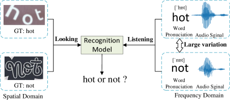
Figure 1: Audio information can provide the salient information for guiding text recognition.

To address this issue, we attempt to use audio information to guide the scene text recognition. In fact, as shown in Figure 1, a single character such as “h” or “n” may not have a significant difference simply based on the visual appearance, as scene text could be presented with various fonts, vague, perspective distortion, etc; however, such error may result in completely different of the pronunciation of the entire word. Recently, using audio information to assist vision tasks have been proven effective [57, 6, 7, 65], e.g., Tian et al.  [56]. show that using audio-visual integration can strengthen the perception ability and thus improve the robustness of audio-visual models. Tang et al.  [55] uses an Automatic Speech Recognition (ASR) model [4, 1] to convert annotations from audio modal to text modal for text spotting tasks, and accelerate the annotation procedure. To the best of our knowledge, few methods consider using audio information for guiding scene text recognition.

In this paper, we propose a novel module, termed AudioOCR, using a transformer-based probabilistic audio decoder for spectrogram sequence prediction. It can be easily plugged into the existing approaches only during the training phase, and thus it brings no extra cost to the baseline model yet introduces obvious improvement. To enable the training, as shown in Figure 4, we adopt a PaddleSpeech [69] engine to convert the text label to the target of mel spectrogram recognition. The text labels are directly from the existing synthesized datasets like MJ [19] and ST [14], which are commonly served as standard training data for scene text recognition. The underlying principle of our method is that the text always has the correct pronunciation regardless of its shape, size, clarity, etc. We summarize our method as follows:

• We discovered a new approach, termed AudioOCR, whereby speech information can supplement text recognition, paving the way for further advances in the field.

• The simplicity of our AudioOCR allows it to be applied to the existing approaches, i.e., it can apparently improve the performance of the recognizers, incurring acceptable computational overhead during the training phase and none whatsoever during the testing phase.

• We evaluate our method by integrating the AudioOCR into 7 previous scene text recognition methods on 12 benchmarks including regular, irregular, and occluded datasets, which demonstrates our method can improve the performance of each recognition method by an average of 1.75% in terms of the recognition accuracy.

2 Related Works

Visual-audio modeling. In the visual-audio domain, there are several advancements that happened in visual-audio encoders in the past. Qu et al. [40] proposed an encoder-decoder architecture LipSound2 which directly predicts mel-scale spectrogram from raw face sequences. Chung et al. [10] proposed a ‘Watch, Listen, Attend and Spell’ (WLAS) network that learns to transcribe videos of mouth motion to characters for lip reading. Arandjelovic et al. [2] designed new network architectures that can be trained for cross-modal retrieval and localizing the sound source in an image through audio-visual correspondence tasks. Oh et al. [36] proposed Speech2Face model for reconstructing a facial image of a person from a short audio recording of that person speaking.

Text-audio modeling. In the text-audio domain, it’s a rapidly evolving field with ongoing research in many different areas, such as Automatic Speech Recognition (ASR) [15, 9, 4, 27] and Text-to-Speech (TTS) Synthesis [63, 53, 43, 41].

Compared to the visual-audio and text-audio domain, our method is different in several aspects: 1) The audio-decoder is a Transformer-based model that is parallelly trained via self-attention mechanism; 2) our method takes the input of visual modality and outputs the audio modality information; 3) our method develops a simple yet effective plug-and-play pipeline specifically designed for OCR, which does not introduce computational overheads in inference stage.

Scene text recognition. Scene text recognition has been an active and challenging research topic in the field of computer vision. The popular methods have relied on encoder-decoder architectures [13, 52, 33, 3, 62, 5, 61, 66, 5], and recent approaches have utilized convolutional neural networks (CNNs) as encoders, followed by recurrent neural networks (RNNs) or connectionist temporal classification (CTC) for decoding [17, 45, 52]. Then attention mechanisms [24] and spatial transformer networks [46, 47] based methods have been proposed to handle irregular text with arbitrary shapes and rotations. Apart from this, some methods [28, 60] attempt to recognize text via character segmentation.

Recently, some methods tend to leverage auxiliary information to assist the recognition process [67, 64, 11, 39, 12, 54, 34], such as the linguistic knowledge. SRN [67] introduces a global semantic reasoning module to refine vision model predictions. SEED [39] designs a semantic module, supervised by embedding outputs of a pretrained language model. Fang et al. [12] propose a method that is based entirely on CNN for both vision and language models. ABINet [11] utilizes a bidirectional network as the language model and an explicit language model by blocking gradient flow. Besides, Song et al. [50] mask random characters in the visual model and restore them by language model to learn linguistic knowledge in a union.

As shown above, previous works mainly leverage linguistic knowledge to assist recognition task; however, audio, another meaningful information is less studied in the literature. Thus, we explicitly utilize audio information through automatic generation without extra annotation costs.

3 Methodology

In this section, we first introduce the overall architecture of the proposed audio guided text recognition framework. Then, we elaborate on the proposed plug-and-play audio decoder, termed AudioOCR, and further analyze the advantages of audio in feature modeling. Finally, we describe the details of the generation of the mel spectrogram of the audio decoder as well as the training process of cooperating with existing recognition methods.

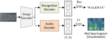
Figure 2: The pipeline of audio guided text recognition method. AudioOCR consists of the image encoder, the recognition decoder, and the pluggable audio decoder for guiding text recognition. Dashed arrows are the training-only operators. Solid arrows indicate forward pass in both training and inference.

3.1 Audio Guided Text Recognition

Our main objective is to precisely recognize each character in images with the help of not only looking but also listening. To this end, we jointly train a simple audio decoder with existing methods to predict the spectrogram of the audio of the corresponding transcription. As shown in Figure 2, our proposed audio-guided text recognition architecture is composed of an image encoder, a recognition decoder, and an audio decoder.

Given an input image $\mathbf{X}$, the image encoder generates visual image embeddings $\mathbf{\hat{X}}$, which is formulated as follows:

$$\mathbf{\hat{X}}=\mathtt{ImageEncoder}\left(\mathbf{X}\leavevmode\nobreak\ ;\Theta_{\text{enc}}\right)\,,$$ (1)

where $\mathbf{X}\in\mathbb{R}^{H^{\prime}\times W^{\prime}\times 3}$ denotes the vector of input image, $H^{\prime}$ and $W^{\prime}$ represent the height and width of image, respectively. $\mathbf{\hat{X}}\in\mathbb{R}^{H\times W\times d_{model}}$ represents the output of the image encoder, and $d_{model}$ indicates the dimension of model. $\mathbf{\hat{X}}$ will be used as input for the recognition decoder and audio decoder. $\Theta_{\text{enc}}$ represents the parameters of the image encoder. In practice, image encoder, depending on different recognizers, can be instantiated into a wide variety of model structures, which usually includes the CNN based e.g. ResNet [16] and transformer [58] based image encoder along with the extra module e.g., flexible rectification [47].

The recognition decoder receives the visual image embedding $\mathbf{\hat{X}}$ to produce a sequence of predicted characters $\hat{Y}=\{y_{1},y_{2},\ldots,y_{n}\}$, in which $n$ is the length of predicted sequence and $y_{i}$ is the $i$-th predicted characters, which can be expressed as:

$$\hat{Y}=\mathtt{RecoDecoder}\left(\mathbf{\hat{X}}\leavevmode\nobreak\ ;\Theta_{\text{rec}}\right)\,,$$ (2)

where RecoDecoder means the recognition decoder module, and $\Theta_{\text{rec}}$ represents the parameters of the recognition decoder.

In practice, there are three types of recognition decoders commonly used in real scenarios, including (1) Connectionist Temporal Classification (CTC) [13, 45]; (2) attention-based sequence prediction (Attn) [47, 26]; and (3) transformer decoder based sequence prediction (Trans) [25, 31, 37]. CTC allows for the prediction of a non-fixed number of a sequence even though a fixed number of the features are given. Attn-based decoder automatically captures the information flow within the input sequence to predict the output sequence. It enables a text recognition model to learn a character-level language model representing output class dependencies. Trans-based decoder leverages self-attention to model long-range dependency between features and predicts the characters of the sequence via an auto-regressive manner.

3.2 Audio Decoder

The audio decoder, as shown in Figure 3, is proposed to guide the recognizers to capture audio modal information. It consists of a Prenet, a visual-audio decoder, and a Mel Linear.

Prenet is composed of two fully connected layers (each has 256 hidden units) with ReLU activation. Prenet is responsible for projecting mel spectrograms into the phoneme subspace of audio, and thus the similarity of a phoneme and mel frame pair can be measured to force the following visual-audio decoder to easily capture visual and audio interaction, which is defined as:

$$\mathbf{\hat{Z}}=\mathtt{Prenet}\left(\mathbf{\dot{Z}}\leavevmode\nobreak\ ;\Theta_{\text{pre}}\right)\,,$$ (3)

where $\mathbf{\dot{Z}}$ is the shifted-right format [58] of the mel spectrogram $\mathbf{Z}\in\mathbb{R}^{T\times 80}$ (Sec. 3.3 describes the generation way), where $T$ is the time length of audio. $\mathbf{\hat{Z}}\in\mathbb{R}^{T\times 256}$ denotes the transformed vector of mel spectrogram containing compact and low dimensional subspace features of audio. $\Theta_{\text{pre}}$ represents the parameters of the Prenet.

The visual-audio decoder is implemented by the transformer decoder. It utilizes the mel spectrogram features $\mathbf{\hat{Z}}$ as query and image embeddings $\mathbf{\hat{X}}$ as key and value to model cross-modal interaction between visual and audio features for learning effective scene text visual representations via cross-attention. The visual-audio decoder hence learns the relationships between visual and audio features. To this end, the visual features $\mathbf{\hat{X}}$ implicitly contain the audio information which is helpful for text recognition of complex scenarios. We add a set of learned positional encoding [58] to mel spectrogram $\mathbf{\hat{Z}}$ for capturing the sequential information, then passing it to visual-audio decoder to refine the mel spectrogram conditioned on visual features:

$$\mathbf{\tilde{Z}}=\mathtt{VADecoder}\left(\mathbf{\mathtt{Q}=\hat{Z},\mathtt{K}=\hat{X},\mathtt{V}=\hat{X}}\leavevmode\nobreak\ ;\Theta_{\text{va}}\right)\,,$$ (4)

where $\mathbf{\tilde{Z}}\in\mathbb{R}^{T\times 256}$ denotes the refined mel spectrogram. VADecoder means the visual-audio decoder. $\Theta_{\text{va}}$ represents the parameters of the visual-audio decoder. In practice, the default settings of the visual-audio decoder consist of $N=3$ stacked decoder layers. Each decoder layer contains a masked multi-head attention, a multi-head attention layer, and an MLP network.

The Mel Linear implemented by a linear projection and the $\mathbf{\tilde{Z}}$ is then used to predict the mel spectrogram, which can be formulated by:

$$\mathbf{\bar{Z}}=\mathtt{MelLinear}\left(\mathbf{\tilde{Z}}\leavevmode\nobreak\ ;\Theta_{\text{mel}}\right)\,,$$ (5)

where $\mathbf{\bar{Z}}\in\mathbb{R}^{T\times 80}$ denotes the predicted mel spectrogram. MelLinear means the Mel Linear. $\Theta_{\text{mel}}$ represents the parameters of the Mel Linear. Then $\mathbf{\bar{Z}}$ and $\mathbf{Z}$ will calculate the L1 loss $L_{mel}$:

$$L_{mel}=\mathtt{L1}\left(\mathbf{\check{Z}}\leavevmode\nobreak\ ,\mathbf{\bar{Z}}\right)\,,$$ (6)

where the mel spectrogram label $\mathbf{\check{Z}}$ and the input of Prenet $\mathbf{\dot{Z}}$ are basically the same (mel spectrogram $\mathbf{Z}$). The only difference is the input $\mathbf{\dot{Z}}$ is the shifted-right format [58] of the $\mathbf{Z}$.

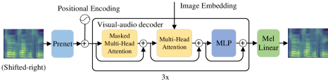
Figure 3: The architecture of the audio decoder. It includes a Prenet, a visual-audio decoder, and a Mel Linear. LayerNorm and Dropout layers are omitted due to space constraints.

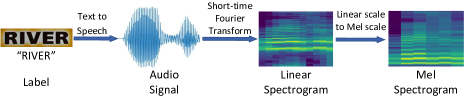
Figure 4: The pipeline of converting the text label to the mel spectrogram used in the audio decoder.

3.3 Mel Spectrogram $\mathbf{Z}$ Generation

Since there is no publicly available dataset that includes text-audio pairs, we use the off-the-shelf text-to-speech tool PaddleSpeech to generate the audio of the transcription of every image and store the audio file with the suffix $.wav$. We then convert the audio data to the mel spectrogram used for the training of the audio decoder.

Specifically, we first get the waveform $\bm{x}$ of the audio from the $.wav$ file, with the shape of $[C,T]$ where $C$ is the number of channels ($C=2$ for stereo audio), and $T$ the number of points used to represent the audio, as shown in Figure 4. Then Short-Time Fourier Transform (STFT) is employed over the waveform $\bm{x}$ to represent audio into a complex-valued tensor of shape $[C,F,L]$ where $F$ is the number of frequencies and $L$ is the length. The STFT is computed on overlapping windowed segments of the waveform $\bm{x}$. The STFT at a point ($f$, $l$) is defined as:

$$\mathtt{STFT}\{\bm{x}\}(f,l)=\sum_{t=0}^{T}\bm{x}_{t}\cdot\bm{w}_{t-l}\cdot\mathtt{exp}\left(-i\frac{2\pi t}{T}f\right)\,,$$ (7)

where $\bm{w}$ is a slide window function of length $W$ that is used to isolate the chunk of interest from the waveform signal. $f$, $l$, and $i$ are frequency, time step, and imaginary part, respectively.

Instead of real and imaginary parts, often the STFT is converted into magnitude and phase, a representation that can be inverted back to real and imaginary parts, and hence back to the waveform. Magnitude, called linear sepctrogram, is defined as $|\mathtt{STFT}\{\bm{x}\}(f,l)|$.

Finally, we perform a mathematical operation on the frequencies of the linear spectrogram to convert the linear scale to the mel scale [51], called mel spectrogram. The reason is that humans do not perceive frequencies on a linear scale [51], and equal distances in mel scale sound equally distant to the listener. The mathematical operation is formulated as:

$$m=2595*\log_{10}\left(1+\frac{f}{700}\right)\,,$$ (8)

where $f$ denotes the linear scale frequency, and $m$ denotes the mel scale frequency. The configuration of mel spectrogram generation refers to appendix.

3.4 Training strategy

Our model is designed to jointly learn with recognition loss and audio loss. The loss function $L$ can be expressed as a weighted sum of the recognition losses and audio losses:

$$L=L_{rec}+\alpha\times L_{mel},$$ (9)

where $L_{rec}$ is the loss for the recognition decoder, and $L_{mel}$ (Eq. 6) is the L1 loss for the audio decoder. According to the numeric values of the losses, $\alpha$ is set to $1.0$ by default.

4 Experiment

We first incorporate the AudioOCR into the existing recognizers to validate its effectiveness. Next, we conduct ablation studies to measure the sensitivity of the designs and generalization ability for AudioOCR.

4.1 Datasets

We use three types of datasets including synthetic datasets, real scene text recognition benchmarks, and our SynthAudio data. Synthetic datasets including MJSynth (MJ) [19], SynthText (ST) [14], and SynAdd (SA) [26]. The details descriptions of the synthetic datasets refer to appendix.

Scene text recognition benchmarks including (1) IIIT5k-Words (IIIT) [32]; (2) Street View Text (SVT) [48] ; (3) ICDAR 2013 (IC13)  [21]; (4) ICDAR 2015 Incidental Text (IC15)  [20]; (5) SVTP-Perspective (SVTP) [38]; (6) CUTE80 (CT80) [44]; (7) COCOText-Validation (COCO) [59]; (8) CTW dataset [30]; (9) Total-Text dataset (TT) [8]; (10) Occlusion Scene Text (OST) [64], including weakly occluded scene text (WOST) and heavily occluded scene text (HOST) are used to evaluate our recognition models; and (11) WordArt dataset [66]. The detailed descriptions of the benchmarks refer to appendix.

SynthAudio data is generated using the open-source text-to-speech toolkit PaddleSpeech [69]. Our corpus is directly from the label of public datasets, including synthetic datasets ST, MJ, real datasets COCO-Text, IIIT5K, SVT, etc. The detailed information of SynthAudio refers to appendix.

4.2 Implementation Details

Our model is implemented based on MMOCR [23]. The model is trained using 4 NVIDIA GTX 3090 GPUs. We choose to perform experiments on the existing reproduced models on MMOCR, including MASTER [31], CRNN [45], SAR [26], SATRN [25], Robust_Scanner (Robust_S) [68], ABINet [11], and ASTER [11], which contains CTC, Attention and Transformer based recognizers.

For the training dataset, we keep the same configuration as the original paper. For different models, we have different data configurations, as shown in Table 1. Unless specified, we set the number of audio decoder layers as 3. We report the word accuracy metric (%) in all experiments.

4.3 Cooperation with Existing Recognizers

As illustrated in Table 1, we validate the benefits of the pluggable AudioOCR for existing recognizers. Specifically, we evaluate AudioOCR by combining it with 7 scene text recognition methods on 12 benchmarks including regular, irregular, and occluded datasets. Equipping with audio decoder methods achieves consistent improvement compared to baseline methods in average recognition accuracy. It is worth mentioning that such improvement is free in the inference stage without introducing any extra costs, while for the training stage, it only brings an additional 4.6 ms/image on average for computation overhead as shown in Table 9.

	Method	Img. data	Audio data	Regular			Irregular						Occluded		WordArt	Avg.
				IIIT5K	SVT	IC13	IC15	SVTP	CT80	CTW	TT	COCO	HOST	WOST
CTC	CRNN-paper	MJ	-	78.2	80.8	86.7	-	-	-	-	-	-	-	-	-	-
	CRNN*	MJ	-	80.5	81.0	86.5	54.1	59.1	55.6	54.3	52.2	37.1	30.1	45.7	33.1	55.8
	CRNN	MJ	600k	82.0	81.0	88.3	57.5	65.4	60.4	55.4	53.5	37.7	36.9	53.0	38.4	59.1
Attention	ASTER-paper	ST+MJ	-	91.9	88.8	89.8	-	74.1	73.3	-	-	-	-	-	-	-
	ASTER*	ST+MJ	-	92.5	89.0	91.2	73.3	80.2	82.3	69.0	69.6	52.3	40.4	61.4	58.2	71.6
	ASTER	ST+MJ	4m	93.7	89.5	93.2	74.7	81.1	86.1	69.8	71.6	53.1	47.8	65.5	60.6	73.9
	SAR-paper	S+R	-	95.0	91.2	94.0	78.8	86.4	89.6	-	-	-	-	-	-	-
	SAR*	S+R	-	95.0	89.6	93.7	79	82.2	88.9	75.6	75.8	63.2	41.4	65.3	63.3	76.1
	SAR	S+R	4m	95.5	90.9	93.5	79.3	82.6	89.9	76.0	78.9	64.3	41.2	65.4	63.4	76.7
	Robust_S-paper	S+R	-	95.4	89.3	94.1	79.2	82.9	89.6	-	-	-	-	-	-	-
	Robust_S*	S+R	-	95.1	89.2	93.1	77.8	80.3	90.3	75.4	75.7	62.0	38.6	65.0	61.0	75.3
	Robust_S	S+R	2m	95.1	90.6	94.1	79.6	81.4	91	75.5	77.9	64.6	42.4	66.1	62.4	76.7
Transformer	SATRN-paper	ST+MJ	-	92.8	91.3	94.1	79	86.5	87.8	-	-	-	-	-	-	-
	SATRN*	ST+MJ	-	94.7	90.7	95.4	81.9	85.7	86.5	75.6	78.4	59.8	56.7	72.0	63.7	78.4
	SATRN	ST+MJ	4m	95.4	92.9	96.6	84.2	88.8	89.9	76.2	79.1	59.9	64.7	76.1	67.5	81.0
	MASTER-paper	ST+MJ+SA	-	95	90.6	95.3	79.4	84.5	87.5	-	-	-	-	-	-	-
	MASTER*	ST+MJ+SA	-	95.3	89.9	95.2	77.0	83.0	89.9	74.2	77.4	54.0	52.2	72.7	65.3	77.2
	MASTER	ST+MJ+SA	4m	95.7	91.2	95.9	79.7	84.7	89.9	75.7	80.2	55.5	52.8	74.2	66.3	78.5
	ABINet-LV-paper	ST+MJ	-	96.2	93.5	97.4	86	89.3	89.2	-	-	-	-	-	-	-
	ABINet-LV*	ST+MJ	-	95.7	94.6	95.7	85.1	89.3	90.3	76.7	81.2	63.7	62.8	76.5	66.7	81.5
	ABINet-LV	ST+MJ	4m	95.9	94.9	97.8	86.1	89.9	91.4	76.8	82.8	64.0	63.5	76.8	66.7	82.3

Table 1: The results of cooperating with existing recognizers. * represents our reproduced results. S+R means ST+MJ+SA+real data. k: one thousand, m: one million. For ABINet, we use the same version of IC13 and IC15 as its paper. In each column, the best performance result of every method is shown in bold font, and the global best result is shown with an underline.

Method	Layers	Img. data	Audio data	Regular			Irregular						Occluded		WordArt	Avg.
				IIIT5K	SVT	IC13	IC15	SVTP	CT80	CTW	TT	COCO	HOST	WOST
CRNN	1	MJ	600k	81.3	79.3	86.8	57.6	62.9	60.4	55.5	51.0	37.3	33.7	48.1	37.0	57.6
CRNN	2	MJ	600k	81.0	80.2	87.8	56.7	62.5	60.1	54.7	52.1	38.0	33.3	48.6	36.4	57.6
CRNN	3	MJ	600k	82.0	81.0	88.3	57.5	65.4	60.4	55.4	53.5	37.7	36.9	53.0	38.4	59.1
CRNN	4	MJ	600k	81.8	80.5	86.7	57.3	62.6	60.4	53.8	52.1	38.2	34.5	47.9	37.3	57.8
ASTER	1	ST+MJ	600k	93.3	88.7	93.0	73.9	80.0	83.7	69.1	70.3	52.7	46.34	65.0	59.6	73.0
ASTER	2	ST+MJ	600k	93.4	87.3	92.0	73.5	79.1	84.7	68.8	70.0	52.3	47.0	65.2	60.2	72.8
ASTER	3	ST+MJ	600k	93.6	89.0	93.0	74.2	80.0	85.4	69.7	71.0	53.1	47.1	65.4	60.2	73.5
ASTER	4	ST+MJ	600k	93.5	88.6	93.0	73.4	79.8	84.0	69.7	70.7	52.2	47.0	65.3	60.1	73.1
ABINet	1	ST+MJ	4m	95.8	94.7	97.3	85.8	89.6	90.3	76.9	81.3	63	62.3	76.3	66.7	81.6
ABINet	2	ST+MJ	4m	95.9	94.6	97.8	85.9	89.5	90.3	76.7	81.2	63.7	62.5	76.4	65.9	81.7
ABINet	3	ST+MJ	4m	95.9	94.9	97.8	86.1	89.9	91.4	76.8	82.8	64	63.5	76.8	66.7	82.2
ABINet	4	ST+MJ	4m	95.4	94.6	97.1	85.7	89.6	91	76.3	81.1	64.7	63.4	76.4	65.7	81.75

Table 2: Ablation study of the depth of the audio decoder layer. Img. and Avg. are short for image and average, respectively. In each column, the best performance result of every method is shown in bold font.

Method	Speaker	Img. data	Audio data	Regular			Irregular						Occluded		WordArt	Avg.
				IIIT5K	SVT	IC13	IC15	SVTP	CT80	CTW	TT	COCO	HOST	WOST
CRNN	Female, British	MJ	600k	82.0	81.0	88.3	57.5	65.4	60.4	55.4	53.5	37.7	36.9	53.0	38.4	59.1
CRNN	Male, British	MJ	600k	81.8	79.9	88.4	57.0	62.6	63.1	54.9	52.3	37.3	33.9	47.6	36.7	58.0
CRNN	Male, American	MJ	600k	81.4	79.3	87.0	55.6	64.0	58.6	55.3	52.4	37.5	33.2	48.8	36.6	57.5
CRNN	Female, American	MJ	600k	82.2	80.4	88.7	57.1	65.5	62.5	54.7	53.6	37.8	36.4	52.6	38.1	59.1
ASTER	Female, British	ST+MJ	600k	93.6	89.0	93.0	74.2	80.0	85.4	69.7	71.0	53.1	47.1	65.4	60.2	73.5
ASTER	Male, British	ST+MJ	600k	93.5	87.1	92.3	73.9	77.5	85.3	69.2	70.3	52.8	47.1	64.6	60.1	72.8
ASTER	Male, American	ST+MJ	600k	93.7	87.3	93.0	73.1	79.2	85.0	69.2	69.6	52.3	46.4	64.6	60.1	72.8
ASTER	Female, American	ST+MJ	600k	93.7	88.1	92.7	73.2	79.3	84.0	69.3	70.6	52.3	47.0	65.4	60.2	73.0
ABINet	Female, British	ST+MJ	4m	95.9	94.9	97.8	86.1	89.9	91.4	76.8	82.8	64.0	63.5	76.8	66.7	82.3
ABINet	Male, British	ST+MJ	4m	95.7	94.7	95.6	84.4	89.6	90.0	77.9	84.2	65.2	61.6	76.2	66.4	81.8
ABINet	Male, American	ST+MJ	4m	95.7	94.6	95.9	84.8	89.5	90.6	77.8	84.3	64.9	61.6	76.4	66.8	82.0
ABINet	Female, American	ST+MJ	4m	95.6	94.2	95.7	84.9	89.9	90.9	78.1	84.5	64.8	61.5	76	65.5	81.8

Table 3: Ablation study of using 4 different accents for the audio information. Img. and Avg. are short for image and average, respectively. In each column, the best performance result of every method is shown in bold font.

Method	Img. data	Audio data	Regular			Irregular						Occluded		WordArt	Avg.
			IIIT5K	SVT	IC13	IC15	SVTP	CT80	CTW	TT	COCO	HOST	WOST
CRNN	MJ	100k	81.0	79.8	87.4	55.3	62.1	57.6	54.6	52.1	37.2	31.1	46.8	35.2	56.7
CRNN	MJ	600k	82.0	81.0	88.3	57.5	65.4	60.4	55.4	53.5	37.7	36.9	53.0	38.4	59.1
CRNN	MJ	4m	81.9	81.2	88.2	57.4	64.5	62.2	55.3	53.4	37.8	36.7	52.2	39.5	59.2
ASTER	ST+MJ	100k	93.2	88.2	93.1	73.9	79.3	82.9	69.2	70.8	53.0	44.8	64.9	59.4	72.7
ASTER	ST+MJ	600k	93.6	89.0	93.0	74.2	80.0	85.4	69.7	71.0	53.1	47.1	65.4	60.2	73.5
ASTER	ST+MJ	4m	93.7	89.5	93.2	74.7	81.1	86.1	69.8	71.6	53.1	47.8	65.5	60.6	73.9
ABINet	ST+MJ	100k	95.7	94.5	97.2	85.7	88.4	90.3	76.4	81.1	63.1	62.2	76.1	66.1	81.4
ABINet	ST+MJ	600k	96.1	94.5	97.8	86.0	88.9	90.3	76.4	81.1	63.7	61.8	76.9	67.6	81.8
ABINet	ST+MJ	4m	95.9	94.9	97.8	86.1	89.9	91.4	76.8	82.8	64.0	63.5	76.8	66.7	82.3

Table 4: Ablation study of the number of the audio data. Img. and Avg. are short for image and average, respectively. In each column, the best performance result of every method is shown in bold font.

Method	Label type	Img. data	Audio data	Regular			Irregular						Occluded		WordArt	Avg.
				IIIT5K	SVT	IC13	IC15	SVTP	CT80	CTW	TT	COCO	HOST	WOST
CRNN	Mel	MJ	600k	82.0	81.0	88.3	57.5	65.4	60.4	55.4	53.5	37.7	36.9	53.0	38.4	59.1
CRNN	Linear	MJ	600k	80.7	80.1	87.0	56.3	62.2	56.6	54.2	51.8	37.6	32.6	48.6	36.1	57.0
ASTER	Mel	ST+MJ	600k	93.6	89.0	93.0	74.2	80.0	85.4	69.7	71.0	53.1	47.1	65.4	60.2	73.5
ASTER	Linear	ST+MJ	600k	93.6	88.0	92.7	73.4	78.5	83.7	68.8	70.5	52.4	46.2	65.3	59.6	72.7
ABINet	Mel	ST+MJ	600k	95.9	94.9	97.8	86.1	89.9	91.4	76.8	82.8	64	63.5	76.8	66.7	82.2
ABINet	Linear	ST+MJ	600k	95.7	94.8	96.9	85.8	89.3	90.5	76.2	81.2	63.8	63.1	75.6	66.7	81.6

Table 5: Ablation study of the spectrogram format. Img. and Avg. are short for image and average, respectively. In each column, the best performance result of every method is shown in bold font.

4.4 Ablation Studies

The number of the audio decoder layers. To study the relationship between the performance and the ability of speech information extraction, we compare the result of models which are implemented with a different number of audio decoder layers $N$. As shown in Table 2, we can see that $N=3$ gets the best performance, and the performance of $N=4$ decreases a lot compared to $N=3$.

The influence of the accents. To examine the influence of the accents, we compare the performance of four different settings: American female accent, American male accent, British female accent, and British male accent. As shown in Table 3, the guidance by the American female and British female audio achieves the best for CRNN, with 3.33% higher than the baseline method in terms of the average accuracy. For ASTER, the best setting is using the British female audio, which is 1.9% higher than the baseline ASTER. Note that for both methods and genders, the American and British accents bring similar gains for the baseline method, while the female accent is clearly more beneficial to the recognizers than the male accent. By analyzing the sound, we find that the female voice is clearer while the male voice is deeper. Reflected in the waveforms, as shown in Figure 5, the female waveform is smoother, clearly identifiable, and may easier to learn. In the following experiments, we adopt the British female audio.

The influence of audio data size. To further demonstrate the effectiveness of audio information, we explore the influence of the audio data volume on text recognition. As shown in Table 4, the increasing amount of data may gradually increase the recognition performance.

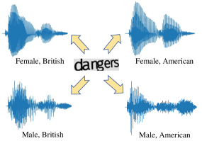
Figure 5: The waveforms of different speakers. The female waveform is smoother and has a higher frequency than the male waveform.

The influence of spectrogram format. We perform a group of experiments on the spectrogram format including linear and mel scale to investigate how it affects the model performance. We report the results in Table 5, which shows that our method achieves the best performance under the mel spectrogram setting compared with linear spectrogram settings on all benchmarks. This is because the mel spectrogram has better discriminant validity for different audios than the linear spectrogram, and thus the audio decoder can easily capture the discrepancy of different text conditioned on the visual features. To this end, the audio decoder can facilitate better learning of discriminatory content by the image encoder.

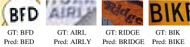
Figure 6: Failure cases of our methods. GT and Pred. represent the ground-truth and the predicted text, respectively.

Input Images	Audio-guided MASTER	MASTER	GT
	SIMENS	SHEIVENS	SIMENS
	Welcome	Welcerne	Welcome
	equip	coulf	equip
	VISA	VINA	VISA

Figure 7: Recognition result samples. Green and red are correct and wrong predictions, respectively. More results are in appendix.

How useful on large-scale real data. As shown in Table 6, based on the large-scale real data TextOCR [49], using 690k audio data of TextOCR can improve CRNN and ABINet from 56.0% to 59.5% and 78.2% to 79.3%, respectively, demonstrating the effectiveness when training on real data.

Usefulness on sentence-level data vs. language modeling methods. Despite the advantages of language modeling, our method provides further enhancement. We examined this using the line-level SROIE [18] dataset and ABINet that possesses language modeling capabilities. Incorporating audio into ABINet increased performance by 5.4% over the original method (92.3% vs. 86.9%), demonstrating its effectiveness for text recognition when handling more sentences for actually text recognition.

Usefulness vs. multiple decoders methods. We assessed the performance of audio decoder against the use of ensemble decoders (CTC+Attention+Transformer) during the training stage. For a fair comparison, the parameters of these additional decoders were matched with those of the audio decoder. Subsequently, inference was carried out using one decoder with MASTER as the baseline. The average accuracy are 78.5% and 77.7%, respectively. This demonstrates the superiority of the proposed audio decoder over using multiple decoders.

			Regular			Irregular						Occluded
Method	Img. ddata	Audio data	IIIT5K	SVT	IC13	IC15	SVTP	CT80	CTW	TT	COCO	HOST	WOST	WordArt	TextOCR	Avg.
CRNN	TextOCR	-	77.4	79.3	88.1	58.1	62.2	61.8	54.9	52.6	41.7	23	41.3	36.3	51.5	56.0
CRNN	TextOCR	690k	78.9	81.9	90.4	62.1	66.4	66.7	56.8	54.6	43.4	29.3	48.8	41.2	53.2	59.5
ABINet	TextOCR	-	85.4	94	93.6	80.3	90.1	90.6	71.3	79.7	63.7	60	72.6	66	70	78.2
ABINet	TextOCR	690k	86.03	94.1	95.4	81.1	89.8	92.1	72.1	80.5	65.2	61.26	75.04	68.2	70.5	79.3

Table 6: Ablation study of training on real data. Img. and Avg. are short for image and average, respectively. In each column, the best performance result of every method is shown in bold font.

Figure 8: Heat map of image features. Best view in screen.

Ablation study on non-English data. Our audio-guided text recognition method, primarily designed and evaluated for English scenarios, has been tested for universality with non-English data as well. Specifically, we selected datasets of images containing scene text in Latin German from MLT19 [35], and Chinese from ReCTS [29]. These German and Chinese datasets comprise diverse pronunciations. We trained CRNN and ABINet on the German and Chinese datasets using the same procedure as for the English dataset. Table 7 shows that our audio-guided method can improve the performance of existing methods by leveraging audio features for multilingual text recognition.

Method	Audio data	MLT19-German	ReCTS-Chinese
CRNN	-	70.6	63.1
CRNN	600k	71.7	64.8
ABINet-LV	-	74.8	81.5
ABINet-LV	60k	75.6	82.6

Table 7: Ablation study on non-English data.

Ablation study on out-of-vocabulary words. Table 8 presents our investigation into the generalization capacity of the audio-guided method for out-of-vocabulary (OOV) data. We designed our OOV experimental setup to ensure that the words in the test set do not exist in the training data, thus facilitating an exploration of the method’s generalization potential. Specifically, we selected French and German words from MLT19, composed solely of alphabetic characters, as our test set to guarantee they do not overlap with the English words in the training set. We utilized existing models trained on English datasets to directly test this set. The results demonstrated consistent improvements offered by AudioOCR. The conducted experiments provide empirical evidence supporting our method’s capacity to generalize to OOV data. It’s suggested that the model might learn pronunciation rules of vowels and consonants from the training data, enabling it to infer unseen words. Moreover, these findings suggest the feasibility of employing minimal audio data for real-world application training, thereby eliminating the need to cover all English words.

Method	French (3,883 imgs)	German (6,916 imgs)
CRNN	70.9	76.1
CRNN+Audio	72.2	76.5
ASTER	77.8	79.9
ASTER+Audio	78.3	82.2
ABINet-LV	85.4	82.2
ABINet-LV+Audio	86.1	82.5

Table 8: Ablation study on out-of-vocabulary words.

Training cost of the proposed auxiliary task. For the training stage of baseline models, as shown in Table 9, using our method introduces an additional 19.4M, 0.44G, and 4.6 ms/image on average, respectively. It is valuable for real applications, since this auxiliary loss is only added during training and the training cost is acceptable, and no additional cost is incurred during the inference phase.

Model	Params(M)	FlOPs(G)	ms/image	Acc. (%)
MASTER	58.98	15.04	122.3	77.2
MASTER+Audio	78.42	15.47	125.8	78.5
ABINet-LV	36.74	5.94	21.8	81.5
ABINet-LV+Audio	56.17	6.39	27.5	82.3

Table 9: The training cost of the proposed auxiliary task.

Analyze the impact of common syllables. We conducted additional experiments with a dataset containing 45 common English prefixes and suffixes used in scene text collected from TT and CTW. We compared the performance of the ABINet method with and without audio. The results showed a 1.5% performance improvement with the addition of audio. This indicates that the audio information, particularly the presence of commonly used syllables, contributes to the enhancement of recognition performance.

Qualitative Analysis. As shown in Figure 7, compared to the baseline methods, audio-guided methods show more robust performance for complicated cases such as blurry or flipping images, distorted, occluded, curved, or art font text. We deduce this may be contributed by the spectrogram of corresponding text features in the frequency domain, which somewhat makes the visual representations more robust. We further visualize failure cases in Figure 6, from which we find the audio-guided recognizers tend to predict phonetically legal words even if the images missing partly characters.

How audio helps improve accuracy? The use of audio information during training enhances the focus of the image encoder on the text areas, thereby boosting its ability to capture subtle visual signals. This is illustrated in Figure 8, where the heat map of the image features highlights larger text areas in both English and Chinese scenarios, even if Chinese has predominantly monosyllabic characters. This audio-visual fusion fortifies the discriminative capability of the image encoder, thereby improving text recognition accuracy. While not involved in inference, the encoder still uses training-derived information to extract relevant features. Hence, the audio decoder aids the recognition process by enriching the encoder with implicit text information.

5 Conclusion

In this work, we propose a simple yet effective plug-and-play module AudioOCR. To exploit the audio knowledge, we design a visual-audio decoder implemented by a transformer to excavate cross-modal information between visual and audio features for learning effective scene text visual representations. It can be easily connected to existing methods during the training phase meanwhile freely improve the performance of recognizers without extra cost in the inference stage. We evaluate the AudioOCR by combining it with 7 scene text recognition methods on 12 benchmarks including regular, irregular, and occluded datasets. The results demonstrate the consistent improvements contributed by the proposed AudioOCR. Besides, it can also deal with more challenging problems including non-English text, out-of-vocabulary words, and text with various accents.

Since the text-to-speech tool, PaddleSpeech, can only handle letters and does not support special symbols for now. The SynthAudio dataset only contains non-special symbolic audio. The improvement of AudioOCR may be further improved if such special symbols can also be guided by the audio, which leaves for future exploration.

As the audio information is naturally connected to the scene text recognition information, the successful attempt of using the AudioOCR further sheds a broad space of cross-modal interaction for scene text recognition.

Appendix A Appendix

A.1 Datasets

MJSynth (MJ) is the synthetic text dataset proposed in [19] a.k.a. Syn90k. The dataset has 9 million images generated from a set of 90k common English words. Every image is annotated with word-level ground-truth. We randomly generate partial corresponding audio according to the text of the images.

SynthText (ST) [14] is a synthetic text dataset originally introduced for text detection. The generating procedure is similar to [19], and the words are rendered onto a full image with a large resolution. 800 thousand full images are used as background images, and usually, each rendered image contains around 10 text lines. It is also widely used for scene text recognition via cropped images. We randomly generated partial corresponding audio according to the text of the images.

SynAdd (SA) is the synthetic text dataset proposed in [26]. The dataset contains 1.6 million word images using the synthetic engine proposed by [19] to compensate for the lack of special characters like punctuations.

The Details of Benchmarks. The detailed descriptions of the benchmarks we used are briefly shown in Table 10.

ID	Benchmarks	Test images	Description
#1	IIIT5K	3,000	regular scene text
#2	SVT	647	regular scene text
#3	IC13	1,015	regular scene text
#4	IC15	1,811	incidental scene text
#5	SVTP	645	perspective scene text
#6	CT80	288	irregular scene text
#7	CTW	1,572	irregular scene text
#8	TT	2,201	irregular scene text
#9	COCO	9,896	incidental scene text
#10	WOST	2,416	weakly occluded scene text
#11	HOST	2,416	heavily occluded scene text
#12	WordArt	1,511	wordart scene text

Table 10: Details of the scene text recognition benchmarks.

The Details of SynthAudio. The detailed information of the SynthAudio can be found in Table 11.

ID	Text Source	Audio Num	Audio Type
#1	MJ	600,000	Female, British
#2	MJ	600,000	Female, American
#3	MJ	600,000	Male, British
#4	MJ	600,000	Male, American
#5	MJ	4,000,000	Female, British
#6	ST	4,000,000	Female, British
#7	COCO	42,142	Female, British
#8	IC11	3,567	Female, British
#9	IC13	848	Female, British
#10	IC15	4,468	Female, British
#11	IIIT5K	2,000	Female, British
#12	TextOCR	690,000	Female, British
#13	MLT19	600,000	Female, German
#14	ReCTS	600,000	Female, Chinese

Table 11: Details of the generated SynthAudio data. British and American represent two different accents.

A.2 Implementation Details

The Details of English and Chinese Audio Generation. We use PaddleSpeech [69] engine to convert the English and Chinese text labels to the audio file via neural network based text to speech (TTS) models. The procedure of TTS models first generates mel spectrograms from text sequences using an acoustic model, and then synthesizes speech from the generated mel spectrograms using a separately trained vocoder. The configurations for audio generation are shown in Table 12. Specifically, we chose Fastspeech2 [42] as our acoustic model, which can remarkably promote the speed of generating audio data. The acoustic model can represent the relationship between an audio signal and the phonemes or other linguistic units that make up speech. The vocoder is used to convert mel spectrograms to an audio waveform. We chose HiFiGAN [22] to be our vocoder since it is commonly used in academic and industrial scenarios. The text corpus is in English and directly from existing synthesized datasets like MJ [19], ST [14], and real data including COCO-Text, IC11, IC13, IC15, IIIT5K, TextOCR, and ReCTS-Chinese [29], which are commonly served as training data for scene text recognition. The generated audio will be used to generate the mel spectrogram $\mathbf{Z}$.

The Details of German Audio Generation. Because PaddleSpeech does not support German audio generation, we use Google Text-to-Speech API engine to convert the German text label to the audio file including MLT19-German [35]. The configuration of the Google Text-to-Speech API is depicted in Table 13.

The Details of Mel Spectrogram Generation. The generation configurations of the mel spectrogram $\mathbf{Z}$ are shown in Table 14. The sample ratio reflects the frequency we sample from the original audio signal, a higher sample ratio tends to deliver a better-quality audio reproduction. Here we set it to 22050, which means we sample 22050 times in one second. For the window function in Eq. 10, we set the window stride to 275.625 (ms) and the window length $W$ to 1102.5 (ms), which decides how many times we compute the Fast Fourier Transform (FFT) on the origin audio signal, and the dimension of FFT is set to 2048. The dimension of the mel spectrogram $F$ is set to 80. The higher the dimension of the mel spectrogram is, the more information can be learned from the audio data, but it also brings extra computation costs.

$$\mathtt{STFT}\{\bm{x}\}(f,l)=\sum_{t=0}^{T}\bm{x}_{t}\cdot\bm{w}_{t-l}\cdot\mathtt{exp}\left(-i\frac{2\pi t}{T}f\right)\,.$$ (10)

Parameters	Configuration
Acoustic Model	Fastspeech2
Vocoder	HiFiGAN
Text Corpus	MJ+ST+Real
Language	English/Chinese

Table 12: The configurations of PaddleSpeech for English/Chinese audio generation. Real consists of COCO, IC11, IC13, IC15, IIIT5K, TextOCR, and ReCTS-Chinese [29].

Parameters	Configuration
Voice Type	Neural2
Language Code	de-DE
Voice Name	de-DE-Neural2-F
SSML Gender	FEMALE
Text Corpus	MLT19-German
Language	German

Table 13: The configurations of Google Text-to-Speech API for German audio generation.

Parameters	Configuration
Sample Ratio (SR)	22050
Window Stride	275.625 (ms)
Window Length $W$	1102.5 (ms)
Dimension of FFT	2048
Dimension of Mel Spectrogram $F$	80

Table 14: The generation configurations of the mel spectrogram $\mathbf{Z}$.

A.3 More Results.

Ablation study for the weight of losses. As shown in Table 15, we vary the trade-off audio loss weight $\alpha$ ranging in [0.5, 1, 2], observing that $\alpha=1$ can get the best performance. We guess that $\alpha=2$ may break the balance between visual information and audio information, and $\alpha=0.5$ results in insufficient training using the audio feature.

Qualitative Analysis. Fig. 9 are more qualitative samples of recognition results of audio-guided and original methods.

Method	Loss weight	Img. data	Audio data	Regular			Irregular						Occluded		WordArt	Avg.
				IIIT5K	SVT	IC13	IC15	SVTP	CT80	CTW	TT	COCO	HOST	WOST
CRNN	1	MJ	600k	82.0	81.0	88.3	57.5	65.4	60.4	55.4	53.5	37.7	36.9	53.0	38.4	59.1
CRNN	2	MJ	600k	81.2	80.2	87.2	56.7	62.2	58.7	54.8	52.1	37.5	33.6	48.5	35.4	57.3
CRNN	0.5	MJ	600k	81.3	80.6	87.0	57.3	62.3	60.1	55.6	52.5	37.3	34.3	49.2	37.7	57.9
ABINet	1	ST+MJ	4m	95.9	94.9	97.8	86.1	89.9	91.4	76.8	82.8	64	63.5	76.8	66.7	82.2
ABINet	2	ST+MJ	4m	95.8	94.9	96	85.8	89.6	90.3	76.9	81.6	63.4	63.1	76.8	66.7	81.7
ABINet	0.5	ST+MJ	4m	95.8	94.7	96.9	85.3	89.8	90.2	76.7	81.4	63.9	62.9	76.5	66.5	81.7

Table 15: Ablation study of loss weight of audio decoder. Img. and Avg. are short for image and average, respectively. In each column, the best performance result of every method is shown in bold font.

Input Images	Audio-guided MASTER	MASTER	GT
	DEPARTMENT	SARTMENT	DEPARTMENT
	EXTRA	EXTRN	EXTRA
	everyone	eucyone	everyone
	own	owy	own
	island	isenndd	island
	alexandra	alexandia	alexandra
	WORLD	140.1221.21	WORLD

Figure 9: Samples of recognition results of audio-guided and original methods. Green and red characters represent correct and wrong predictions, respectively.

References

- [1] Dario Amodei, Sundaram Ananthanarayanan, Rishita Anubhai, Jin Bai, Eric Battenberg, Carl Case, Jared Casper, Bryan Catanzaro, Jingdong Chen, Mike Chrzanowski, Adam Coates, Gregory Frederick Diamos, Erich Elsen, Jesse Engel, Linxi (Jim) Fan, Christopher Fougner, Awni Y. Hannun, Billy Jun, Tony Xiao Han, Patrick LeGresley, Xiangang Li, Libby Lin, Sharan Narang, A. Ng, Sherjil Ozair, Ryan J. Prenger, Sheng Qian, Jonathan Raiman, Sanjeev Satheesh, David Seetapun, Shubho Sengupta, Anuroop Sriram, Chong-Jun Wang, Yi Wang, Zhiqian Wang, Bo Xiao, Yan Xie, Dani Yogatama, Junni Zhan, and Zhenyao Zhu. Deep speech 2 : End-to-end speech recognition in english and mandarin. In ICML, pages 173–182, 2016.
- [2] Relja Arandjelović and Andrew Zisserman. Objects that sound. In ECCV, 2018.
- [3] Jeonghun Baek, Geewook Kim, Junyeop Lee, Sungrae Park, Dongyoon Han, Sangdoo Yun, Seong Joon Oh, and Hwalsuk Lee. What is wrong with scene text recognition model comparisons? dataset and model analysis. In 2019 IEEE/CVF International Conference on Computer Vision (ICCV), pages 4714–4722, 2019.
- [4] Alexei Baevski, Henry Zhou, Abdel rahman Mohamed, and Michael Auli. wav2vec 2.0: A framework for self-supervised learning of speech representations. In NeurIPS, 2020.
- [5] Darwin Bautista and Rowel Atienza. Scene text recognition with permuted autoregressive sequence models. In ECCV, 2022.
- [6] Otavio Braga and Olivier Siohan. Best of both worlds: Multi-task audio-visual automatic speech recognition and active speaker detection. ICASSP 2022 - 2022 IEEE International Conference on Acoustics, Speech and Signal Processing (ICASSP), pages 6047–6051, 2022.
- [7] Ying Cheng, Ruize Wang, Zhihao Pan, Rui Feng, and Yuejie Zhang. Look, listen, and attend: Co-attention network for self-supervised audio-visual representation learning. Proceedings of the 28th ACM International Conference on Multimedia, 2020.
- [8] Chee-Kheng Chng and Chee Seng Chan. Total-text: A comprehensive dataset for scene text detection and recognition. In 2017 14th IAPR International Conference on Document Analysis and Recognition (ICDAR), volume 01, pages 935–942, 2017.
- [9] Jan Chorowski, Dzmitry Bahdanau, Dmitriy Serdyuk, Kyunghyun Cho, and Yoshua Bengio. Attention-based models for speech recognition. In NeurIPS, 2015.
- [10] Joon Son Chung, Andrew W. Senior, Oriol Vinyals, and Andrew Zisserman. Lip reading sentences in the wild. In 2017 IEEE Conference on Computer Vision and Pattern Recognition (CVPR), pages 3444–3453, 2016.
- [11] Shancheng Fang, Hongtao Xie, Yuxin Wang, Zhendong Mao, and Yongdong Zhang. Read like humans: Autonomous, bidirectional and iterative language modeling for scene text recognition. In CVPR, pages 7098–7107, 2021.
- [12] Shancheng Fang, Hongtao Xie, Zheng-Jun Zha, Nannan Sun, Jianlong Tan, and Yongdong Zhang. Attention and language ensemble for scene text recognition with convolutional sequence modeling. In Proceedings of the 26th ACM International Conference on Multimedia, MM ’18, page 248–256, New York, NY, USA, 2018. Association for Computing Machinery.
- [13] Alex Graves, Santiago Fernández, Faustino Gomez, and Jürgen Schmidhuber. Connectionist temporal classification: labelling unsegmented sequence data with recurrent neural networks. In International Conference on Machine Learning, pages 369–376, 2006.
- [14] Ankush Gupta, Andrea Vedaldi, and Andrew Zisserman. Synthetic data for text localisation in natural images. In Proceedings of the IEEE conference on computer vision and pattern recognition, pages 2315–2324, 2016.
- [15] Awni Y. Hannun, Carl Case, Jared Casper, Bryan Catanzaro, Gregory Frederick Diamos, Erich Elsen, Ryan J. Prenger, Sanjeev Satheesh, Shubho Sengupta, Adam Coates, and A. Ng. Deep speech: Scaling up end-to-end speech recognition. ArXiv, abs/1412.5567, 2014.
- [16] Kaiming He, X. Zhang, Shaoqing Ren, and Jian Sun. Deep residual learning for image recognition. In 2016 IEEE Conference on Computer Vision and Pattern Recognition (CVPR), pages 770–778, 2016.
- [17] Pan He, Weilin Huang, Yu Qiao, Chen Change Loy, and Xiaoou Tang. Reading scene text in deep convolutional sequences. In AAAI, pages 3501–3508, 2016.
- [18] Zheng Huang, Kai Chen, Jianhua He, Xiang Bai, Dimosthenis Karatzas, Shijian Lu, and CV Jawahar. Icdar2019 competition on scanned receipt ocr and information extraction. In 2019 International Conference on Document Analysis and Recognition (ICDAR), pages 1516–1520. IEEE, 2019.
- [19] Max Jaderberg, Karen Simonyan, Andrea Vedaldi, and Andrew Zisserman. Synthetic data and artificial neural networks for natural scene text recognition. In NeurIPS Workshop, 2014.
- [20] Dimosthenis Karatzas, Lluís Gómez i Bigorda, Anguelos Nicolaou, Suman K. Ghosh, Andrew D. Bagdanov, M. Iwamura, Jiri Matas, Lukás Neumann, Vijay Ramaseshan Chandrasekhar, Shijian Lu, Faisal Shafait, Seiichi Uchida, and Ernest Valveny. Icdar 2015 competition on robust reading. In 2015 13th International Conference on Document Analysis and Recognition (ICDAR), pages 1156–1160, 2015.
- [21] Dimosthenis Karatzas, Faisal Shafait, Seiichi Uchida, M. Iwamura, Lluís Gómez i Bigorda, Sergi Robles Mestre, Joan Mas Romeu, David Fernández Mota, Jon Almazán, and Lluís-Pere de las Heras. Icdar 2013 robust reading competition. In 2013 12th International Conference on Document Analysis and Recognition, pages 1484–1493, 2013.
- [22] Jungil Kong, Jaehyeon Kim, and Jaekyoung Bae. Hifi-gan: Generative adversarial networks for efficient and high fidelity speech synthesis. In NeurIPS, page 17022–17033, 2020.
- [23] Zhanghui Kuang, Hongbin Sun, Zhizhong Li, Xiaoyu Yue, Tsui Hin Lin, Jianyong Chen, Huaqiang Wei, Yiqin Zhu, Tong Gao, Wenwei Zhang, Kai Chen, Wayne Zhang, and Dahua Lin. Mmocr: A comprehensive toolbox for text detection, recognition and understanding. In Proceedings of the 29th ACM International Conference on Multimedia, 2021.
- [24] Chen-Yu Lee and Simon Osindero. Recursive recurrent nets with attention modeling for ocr in the wild. In Computer Vision and Pattern Recognition, pages 2231–2239, 2016.
- [25] Junyeop Lee, Sungrae Park, Jeonghun Baek, Seong Joon Oh, Seonghyeon Kim, and Hwalsuk Lee. On recognizing texts of arbitrary shapes with 2d self-attention. In 2020 IEEE/CVF Conference on Computer Vision and Pattern Recognition Workshops (CVPRW), pages 2326–2335, 2020.
- [26] Hui Li, Peng Wang, Chunhua Shen, and Guyu Zhang. Show, attend and read: A simple and strong baseline for irregular text recognition. In AAAI, page 8610–8617, 2019.
- [27] Jinyu Li. Recent advances in end-to-end automatic speech recognition. APSIPA Transactions on Signal and Information Processing, 2022.
- [28] Minghui Liao, Jian Zhang, Zhaoyi Wan, Fengming Xie, Jiajun Liang, Pengyuan Lyu, Cong Yao, and Xiang Bai. Scene text recognition from two-dimensional perspective. In AAAI, page 8714–8721, 2019.
- [29] Xi Liu, Rui Zhang, Yongsheng Zhou, Qianyi Jiang, Qi Song, Nan Li, Kai Zhou, Lei Wang, Dong Wang, Minghui Liao, Mingkun Yang, Xiang Bai, Baoguang Shi, Dimosthenis Karatzas, Shijian Lu, and C. V. Jawahar. Icdar 2019 robust reading challenge on reading chinese text on signboard. In 2019 International Conference on Document Analysis and Recognition (ICDAR), pages 1577–1581, 2019.
- [30] Yuliang Liu, Lianwen Jin, Shuaitao Zhang, Canjie Luo, and Sheng Zhang. Curved scene text detection via transverse and longitudinal sequence connection. Pattern Recognit., 90:337–345, 2019.
- [31] Ning Lu, Wenwen Yu, Xianbiao Qi, Yihao Chen, Ping Gong, and Rong Xiao. Master: Multi-aspect non-local network for scene text recognition. Pattern Recognit., 117:107980, 2021.
- [32] Anand Mishra, Karteek Alahari, and CV Jawahar. Top-down and bottom-up cues for scene text recognition. In 2012 IEEE Conference on Computer Vision and Pattern Recognition, pages 2687–2694. IEEE, 2012.
- [33] Anand Mishra, Karteek Alahari, and C. V. Jawahar. Enhancing energy minimization framework for scene text recognition with top-down cues. Computer Vision and Image Understanding, pages 30–42, 2016.
- [34] Byeonghu Na, Yoonsik Kim, and Sungrae Park. Multi-modal text recognition networks: Interactive enhancements between visual and semantic features. In European Conference on Computer Vision, 2022.
- [35] Nibal Nayef, Yash Patel, Michal Busta, Pinaki Nath Chowdhury, Dimosthenis Karatzas, Wafa Khlif, Jiri Matas, Umapada Pal, Jean-Christophe Burie, Cheng-Lin Liu, and Jean-Marc Ogier. Icdar2019 robust reading challenge on multi-lingual scene text detection and recognition — rrc-mlt-2019. In 2019 International Conference on Document Analysis and Recognition (ICDAR), pages 1582–1587, 2019.
- [36] Tae-Hyun Oh, Tali Dekel, Changil Kim, Inbar Mosseri, William T. Freeman, Michael Rubinstein, and Wojciech Matusik. Speech2face: Learning the face behind a voice. In 2019 IEEE/CVF Conference on Computer Vision and Pattern Recognition (CVPR), pages 7531–7540, 2019.
- [37] Dezhi Peng, Xinyu Wang, Yuliang Liu, Jiaxin Zhang, Mingxin Huang, Songxuan Lai, Jing Li, Shenggao Zhu, Dahua Lin, Chunhua Shen, et al. Spts: single-point text spotting. In Proceedings of the 30th ACM International Conference on Multimedia, pages 4272–4281, 2022.
- [38] Trung Quy Phan, Palaiahnakote Shivakumara, Shangxuan Tian, and Chew Lim Tan. Recognizing text with perspective distortion in natural scenes. In 2013 IEEE International Conference on Computer Vision, pages 569–576, 2013.
- [39] Zhi Qiao, Y. Zhou, Dongbao Yang, Yucan Zhou, and Weiping Wang. Seed: Semantics enhanced encoder-decoder framework for scene text recognition. In 2020 IEEE/CVF Conference on Computer Vision and Pattern Recognition (CVPR), pages 13525–13534, 2020.
- [40] Leyuan Qu, Cornelius Weber, and Stefan Wermter. Lipsound2: Self-supervised pre-training for lip-to-speech reconstruction and lip reading. IEEE transactions on neural networks and learning systems, PP, 2021.
- [41] Yi Ren, Chenxu Hu, Xu Tan, Tao Qin, Sheng Zhao, Zhou Zhao, and Tie-Yan Liu. Fastspeech 2: Fast and high-quality end-to-end text to speech. In ICLR, 2021.
- [42] Yi Ren, Chenxu Hu, Xu Tan, Tao Qin, Sheng Zhao, Zhou Zhao, and Tie-Yan Liu. Fastspeech 2: Fast and high-quality end-to-end text to speech. In ICLR, 2021.
- [43] Yi Ren, Yangjun Ruan, Xu Tan, Tao Qin, Sheng Zhao, Zhou Zhao, and Tie-Yan Liu. Fastspeech: Fast, robust and controllable text to speech. In NeurIPS, 2019.
- [44] Anhar Risnumawan, Palaiahnakote Shivakumara, Chee Seng Chan, and Chew Lim Tan. A robust arbitrary text detection system for natural scene images. Expert Syst. Appl., 41:8027–8048, 2014.
- [45] Baoguang Shi, Xiang Bai, and Cong Yao. An end-to-end trainable neural network for image-based sequence recognition and its application to scene text recognition. IEEE Transactions on Pattern Analysis and Machine Intelligence, pages 2298–2304, 2015.
- [46] Baoguang Shi, Xinggang Wang, Pengyuan Lyu, Cong Yao, and Xiang Bai. Robust scene text recognition with automatic rectification. In CVPR, pages 4168–4176, 2016.
- [47] Baoguang Shi, Mingkun Yang, Xinggang Wang, Pengyuan Lyu, Cong Yao, and Xiang Bai. Aster: An attentional scene text recognizer with flexible rectification. IEEE Transactions on Pattern Analysis and Machine Intelligence, pages 2035–2048, 2019.
- [48] Cunzhao Shi, Chunheng Wang, Baihua Xiao, Song Gao, and Jinlong Hu. End-to-end scene text recognition using tree-structured models. Pattern Recognit., 47:2853–2866, 2014.
- [49] Amanpreet Singh, Guan Pang, Mandy Toh, Jing Huang, Wojciech Galuba, and Tal Hassner. Textocr: Towards large-scale end-to-end reasoning for arbitrary-shaped scene text. In Proceedings of the IEEE/CVF Conference on Computer Vision and Pattern Recognition, pages 8802–8812, 2021.
- [50] Sibo Song, Jianqiang Wan, Zhibo Yang, Jun Tang, Wenqing Cheng, Xiang Bai, and Cong Yao. Vision-language pre-training for boosting scene text detectors. In CVPR, 2022.
- [51] S. S. Stevens, John E. Volkmann, and Edwin B. Newman. A scale for the measurement of the psychological magnitude pitch. Journal of the Acoustical Society of America, 8:185–190, 1937.
- [52] Bolan Su and Shijian Lu. Accurate recognition of words in scenes without character segmentation using recurrent neural network. Pattern Recognition, pages 397–405, 2017.
- [53] Hideyuki Tachibana, Katsuya Uenoyama, and Shunsuke Aihara. Efficiently trainable text-to-speech system based on deep convolutional networks with guided attention. In 2018 IEEE International Conference on Acoustics, Speech and Signal Processing (ICASSP), pages 4784–4788, 2017.
- [54] Yew Lee Tan, Adams Wai-Kin Kong, and Jung-Jae Kim. Pure transformer with integrated experts for scene text recognition. In ECCV, 2022.
- [55] Jing Rui Tang, Su Qiao, Benlei Cui, Yuhang Ma, Sheng Zhang, and D. Kanoulas. You can even annotate text with voice: Transcription-only-supervised text spotting. In Proceedings of the 30th ACM International Conference on Multimedia, pages 4154–4163, 2022.
- [56] Yapeng Tian and Chenliang Xu. Can audio-visual integration strengthen robustness under multimodal attacks? In 2021 IEEE/CVF Conference on Computer Vision and Pattern Recognition (CVPR), pages 5597–5607, 2021.
- [57] Arun Balajee Vasudevan, Dengxin Dai, and Luc Van Gool. Sound and visual representation learning with multiple pretraining tasks. In 2022 IEEE/CVF Conference on Computer Vision and Pattern Recognition (CVPR), pages 14596–14606, 2022.
- [58] Ashish Vaswani, Noam M. Shazeer, Niki Parmar, Jakob Uszkoreit, Llion Jones, Aidan N. Gomez, Lukasz Kaiser, and Illia Polosukhin. Attention is all you need. In NeurIPS, volume 30. Curran Associates, Inc., 2017.
- [59] Andreas Veit, Tomas Matera, Lukás Neumann, Jiri Matas, and Serge J. Belongie. Coco-text: Dataset and benchmark for text detection and recognition in natural images. ArXiv, abs/1601.07140, 2016.
- [60] Zhaoyi Wan, Minghang He, Haoran Chen, Xiang Bai, and Cong Yao. Textscanner: Reading characters in order for robust scene text recognition. In AAAI, pages 12120–12127, 2020.
- [61] P. Wang, Cheng Da, and Cong Yao. Multi-granularity prediction for scene text recognition. In European Conference on Computer Vision, 2022.
- [62] Tianwei Wang, Yuanzhi Zhu, Lianwen Jin, Canjie Luo, Xiaoxue Chen, Y. Wu, Qianying Wang, and Mingxiang Cai. Decoupled attention network for text recognition. In AAAI, pages 12216–12224, 2020.
- [63] Yuxuan Wang, R. J. Skerry-Ryan, Daisy Stanton, Yonghui Wu, Ron J. Weiss, Navdeep Jaitly, Zongheng Yang, Ying Xiao, Z. Chen, Samy Bengio, Quoc V. Le, Yannis Agiomyrgiannakis, Robert A. J. Clark, and Rif A. Saurous. Tacotron: Towards end-to-end speech synthesis. In Interspeech, 2017.
- [64] Yuxin Wang, Hongtao Xie, Shancheng Fang, Jing Wang, Shenggao Zhu, and Yongdong Zhang. From two to one: A new scene text recognizer with visual language modeling network. In 2021 IEEE/CVF International Conference on Computer Vision (ICCV), pages 14174–14183, 2021.
- [65] Peng Wu, Jing Liu, Yujiao Shi, Yujia Sun, Fang Shao, Zhaoyang Wu, and Zhiwei Yang. Not only look, but also listen: Learning multimodal violence detection under weak supervision. In ECCV, 2020.
- [66] Xudong Xie, Ling Fu, Zhifei Zhang, Zhaowen Wang, and Xiang Bai. Toward understanding wordart: Corner-guided transformer for scene text recognition. In ECCV, pages 303–323, 2022.
- [67] Deli Yu, Xuan Li, Chengquan Zhang, Junyu Han, Jingtuo Liu, and Errui Ding. Towards accurate scene text recognition with semantic reasoning networks. In 2020 IEEE/CVF Conference on Computer Vision and Pattern Recognition (CVPR), pages 12110–12119, 2020.
- [68] Xiaoyu Yue, Zhanghui Kuang, Chenhao Lin, Hongbin Sun, and Wayne Zhang. Robustscanner: Dynamically enhancing positional clues for robust text recognition. In European Conference on Computer Vision, pages 135–151, 2020.
- [69] Hui Zhang, Tian Yuan, Junkun Chen, and et al. Paddlespeech: An easy-to-use all-in-one speech toolkit. In Proceedings of the 2022 Conference of the North American Chapter of the Association for Computational Linguistics: Human Language Technologies: Demonstrations, page 114–123. Association for Computational Linguistics, 2022.