Generative Modeling of Labeled Graphs under Data Scarcity

Abstract

Deep graph generative modeling has gained enormous attraction in recent years due to its impressive ability to directly learn the underlying hidden graph distribution. Despite their initial success, these techniques, like many of the existing deep generative methods, require a large number of training samples to learn a good model. Unfortunately, a large number of training samples may not always be available in scenarios such as drug discovery for rare diseases. At the same time, recent advances in few-shot learning have opened door to applications where available training data is limited. In this work, we introduce the hitherto unexplored paradigm of labeled graph generative modeling under data scarcity. Towards this, we develop GShot, a meta-learning based framework for labeled graph generative modeling under data scarcity. GShot learns to transfer meta-knowledge from similar auxiliary graph datasets. Utilizing these prior experiences, GShot quickly adapts to an unseen graph dataset through self-paced fine-tuning. Through extensive experiments on datasets from diverse domains having limited training samples, we establish that GShot generates graphs of superior fidelity compared to existing baselines.

1 Introduction and Related Work

With recent advances in deep learning, there has been a surge in developing deep graph generative methods that directly learn the underlying hidden distribution of graphs from the data itself [1, 2, 3, 4, 5, 6, 7, 8, 9, 10]. These techniques have shown significant improvement over the traditional methods for the graph generation task. Since many real-world graphs such as protein interaction networks [11] and drug molecules [12] are labeled and originate from diverse domains, our focus is on learning domain-agnostic, labeled graph generative [2, 13] model which jointly models the relationships between a graph structure and its node/edge labels.

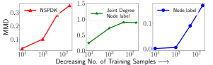
A well-known fact about deep generative models is that they are not well suited for applications where training data is scarce [14]. In our study, we observe similar trends for graph deep generative modeling. In Fig.  1a we study the impact of limiting the number of training samples available to GraphGen [2], which is the state-of-the-art method for domain agnostic labeled graph generation. We observe that GraphGen’s performance deteriorates significantly when the size of the training dataset is reduced.

(a) Performance vs Number of training samples

(b) The pipeline of steps in GShot.

Figure 1: (a) Increase in Maximum Mean Discrepancy (MMD) scores for different graph metrics when the number of training samples (log scale) are decreased in a chemical compound dataset (Dataset #2 in Table 3) for GraphGen [2]. A higher MMD corresponds to poor fidelity. (b) Our proposed architecture.

The lack of training graphs is often severe in many important settings such as effective drug discovery for rare diseases [15] or speedy drug discovery during pandemics such as Covid-19 [16]. Similar issue appears in physics while developing generative models for computationally expensive N-body simulations [17, 18, 19].

In this context, we observe that although the availability of graphs exhibiting a specific desired property may be limited, it may be possible to identify graph repositories exhibiting similar properties. To elaborate, we may not have access to a large set of molecules exhibiting activity against Covid-19. However, million-scale repositories of chemical compounds are widely available [20], from which the broad characteristics of chemical compounds such as valency rules, correlated functional groups, etc. may be learned. Hence, potentially, the learning task from the smaller Covid-19 repository could be focused only on features that are unique to this set. We exploit this intuition and make the following novel contributions:

• Problem Formulation: We formulate the problem of domain-agnostic, labeled graph generative modeling under data scarcity. To the best of our knowledge, we are the first to investigate this problem.

• Algorithm: We propose GShot, that effectively integrates meta-learning with auto-regressive graph generative model to facilitate transfer of knowledge from a set of auxiliary graph datasets to target graph dataset(s). Meta-learning on these auxiliary datasets fosters a high quality parameter initialization. Subsequently, using a self-paced fine-tuning approach, GShot adapts to unseen target graph dataset using a small number of training samples.

• Empirical Evaluation: We perform extensive experiments across multiple real labeled graph datasets spanning a variety of domains such as chemical compounds, proteins, and physical interaction systems. We establish that GShot is effective in learning graph distributions with high fidelity even on datasets containing as few as $50$ training samples, and significantly improves over baselines that learn from scratch.

2 Problem Formulation

Definition 1 (Graph).

A graph is represented as $G=(V,E)$, where $V=\{v_{1},\cdots,v_{n}\}$ is a set of $n$ nodes and $E=\{(v_{i},v_{j})\mid v_{i},v_{j}\in V\}$ is a set of edges. Let $\mathbb{L}_{node}:V\to\mathbb{V}$ and $\mathbb{L}_{edge}:E\to\mathbb{E}$ be the node and edge label mappings respectively where $\mathbb{V}$ and $\mathbb{E}$ are the set of all node and edge labels respectively. We assume that the graph is connected and there are no self-loops.

A graph dataset $D{=}\{G_{1},\cdots,G_{N}\}$ is a collection of $N$ graphs. Graph dataset $D_{1}$ is considered to be an auxiliary dataset of graph dataset $D_{2}$ if $D_{1}$ is similar to $D_{2}$. As discussed in Sec. 1, a generic set of chemical compounds may be considered as an auxiliary dataset to a specific subgroup of compounds that display a desired activity against a virus. In the current context of labeled domain-agnostic graph generative modeling, we below define the concept of graph dataset distance metric and subsequently formally define auxiliary dataset.

Definition 2 (Graph Dataset Distance Metric).

A graph dataset distance metric is a function $\Lambda_{m}(D_{i},D_{j})\mapsto\mathbb{R}$ that takes two graph datasets $D_{i}$ and $D_{j}$ as input and computes distance between the two datasets as per metric $\Lambda_{m}$.

Several metrics have been proposed in the literature for comparing graph datasets [2, 13]. In Sec. 4.1 we describe various distance metrics.

Definition 3 (Auxiliary Dataset).

A graph dataset is considered to be an auxiliary dataset to a target dataset if it satisfies the following conditions:

1. The node/edge label space of the target and auxiliary datasets should be similar.

2. The distances between auxiliary and target graph datasets should be low as per Defn. 2.

Problem 1 (Graph Generative modelling).

The goal of labeled graph generative modeling of a dataset $D$ of graphs is to learn a model, ${p}_{\theta}(D)$, parameterized by $\theta$, that approximates the true latent distribution $p(D)$ of graphs in $D$. The learned generative model is effective if it is capable of generating graphs similar to those in $D$.

The goal is to learn a generative model over a target graph dataset $D_{T}$, where $|D_{T}|$ is small. Since $|D_{T}|$ is small, accurate modeling is hard (Recall Fig. 1a). However, if $D_{T}$ is accompanied with a collection of auxiliary datasets, the generative model should be able to use this knowledge and augment its learning. Formally, it is defined as follows.

Problem 2 (Labeled Graph Generative Modelling under Data Scarcity).

Input: A collection of auxiliary graph datasets $\mathcal{D}{=}\{D_{1},\cdots,D_{\mathcal{B}}\}$ and a target dataset $D_{T}$.
Goal: To learn a graph generative model $p_{\theta}(D)$ that is capable of leveraging the knowledge from $\mathcal{D}$ and effectively adapting to the unseen target dataset $D_{T}$.

Figure 2: Architecture of GShot

3 GShot: Proposed Methodology

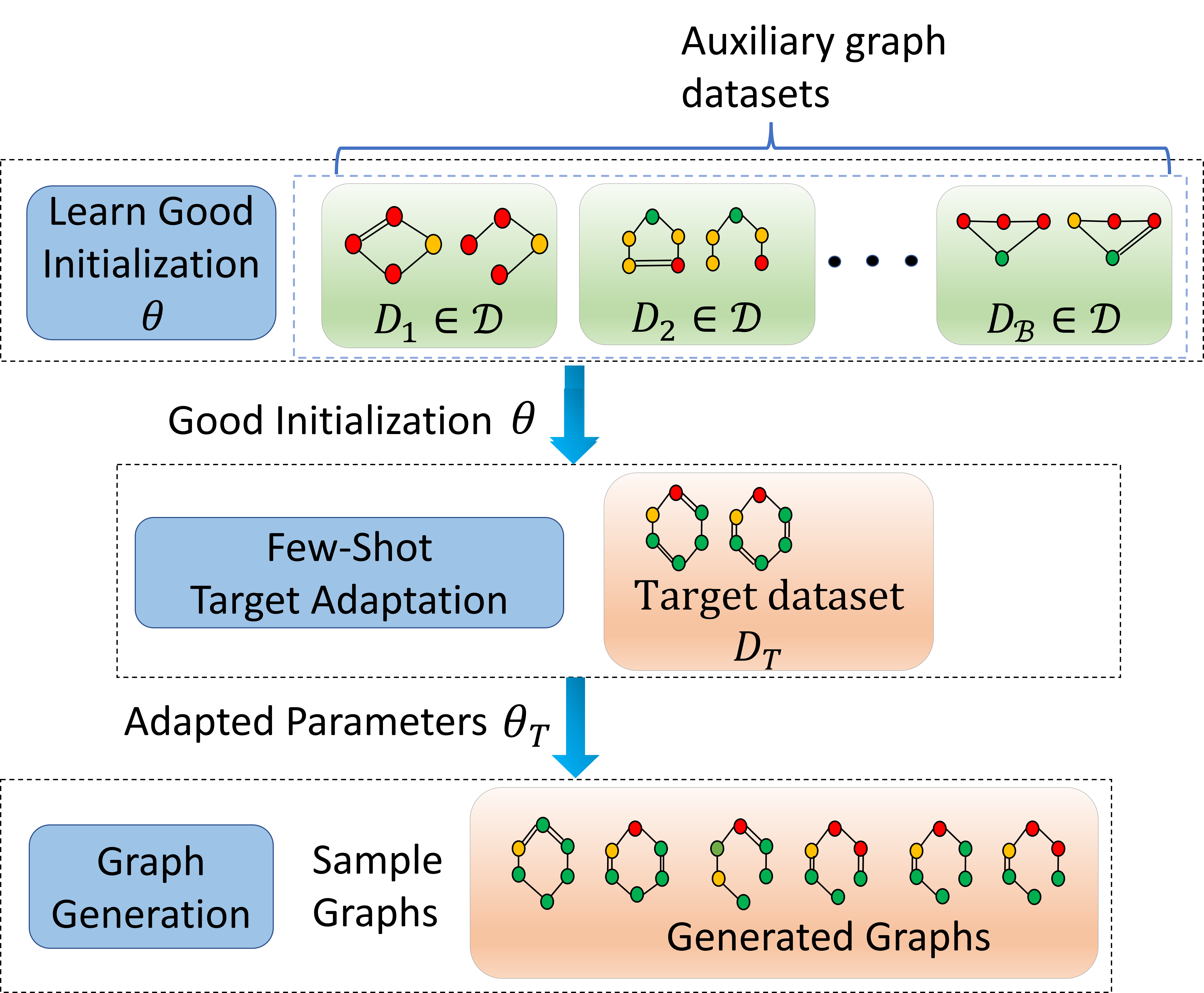
Given a set of auxiliary datasets $D_{1},\cdots,D_{\mathcal{B}}$, first, GShot learns initial model parameters $\theta$. $\theta$ is learned in a strategic manner such that, at inference time, when an unseen target dataset $D_{T}$ containing a small number of graphs are provided as input, we can fine-tune $\theta$ to new $\theta_{{T}}$ where $p_{\theta_{T}}(D_{T})$ best approximates the true distribution of $D_{T}$. Finally, to generate graphs, we sample from $p_{\theta_{T}}(D_{T})$. Fig. 1b provides a visual summary of this approach.

The proposed approach draws inspiration from meta-learning [21, 22]. The main objective of meta-learning is to learn initial model parameters for a set of tasks in such a way that they can be adapted to various unseen target tasks having limited training data. In the context of our problem, each task $\mathcal{T}_{i}$ refers to the graph generative modeling task for dataset $D_{i}$ in the auxiliary dataset $\mathcal{D}$. Each task $\mathcal{T}_{i}$ is associated with a loss function $\mathcal{L}_{{i}}$. During meta-training, the optimal initial parameter $\theta$ is learned using $\mathcal{D}$. Then, given an unseen target task $\mathcal{T}_{T}$ corresponding to unseen graph dataset $D_{T}$ with an associated loss $\mathcal{L}_{{T}}$, $\theta$ is fine-tuned for $\mathcal{L}_{{T}}$ using small number of data samples of $\mathcal{T}_{T}$. When mapped to our problem of graph generative modeling, the loss function measures how well $p_{\theta_{T}}(D_{T})$ mimics the true distribution of $D_{T}$.

3.1 Architecture Overview

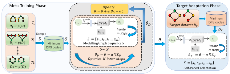
Fig. 2 presents the architecture of GShot. In order to learn a generative model over labeled graphs on a dataset $D$, we first convert graphs to sequences. This conversion allows us to leverage the rich literature on auto-regressive generative models. Auto-regressive methods[2, 13] have obtained superior fidelity and high scalability on domain-agnostic graph generative modeling task. Two popular encoding schemes for encoding graphs into sequence are BFS encoding [13] and DFS encoding [2]. In our work, we choose DFS encoding. This choice is motivated by the observation that minimum DFS codes, which is an instance of DFS encoding, provides one-to-one mapping from graphs to sequences. In contrast, in BFS encoding, the same graph may have multiple sequence representations, and may be exponential in the worst case with respect to the graph size. Consequently, one-to-one mapping is an attractive feature that our model can exploit, and as others have shown, it also improves the scalability and fidelity of graph generative modeling [2].

Once graphs are converted into sequences via minimum DFS codes, as shown in Fig. 2, meta-learning is conducted on the sequence representations to learn parameter set $\theta$. To model sequences, we use LSTM as shown in Fig. 2. Finally, during target-adaptation phase, the target graph database $D_{T}$ is converted to the equivalent sequence representation $\mathcal{S}_{T}$, followed by fine-tuning to learn $\theta_{T}$. To generate graphs, we sample sequences from $p_{\theta_{T}}(\mathcal{S}_{T})$, which are then converted to graphs. The conversion back from a sequence to its graph representation is trivial since our DFS-encoding enables one-to-one mapping. Hence, this conversion can be performed in $O(|E|)$ time, where $E$ is the set of edges. We next deep-dive into each of these individual steps.

3.2 DFS Codes: Graph to Sequence encoding

We first formalize the concept Graph Canonization.

Definition 4 (Graph Isomorphism).

Two graphs $G_{i}=(V_{i},$ $E_{i})$ and $G_{j}=(V_{j},$ $E_{j})$ are said to be isomorphic if there exists a bijection $\phi$ such that for every vertex $v\in V_{i},\;\phi(v)\in V_{j}$ and for every edge $e=(u,v)\in E_{i},\phi(e)=(\phi(u),\phi(v))\in E_{j}$. Furthermore, for labeled graphs to be isomorphic, in addition to above conditions, the labels of mapped nodes and edges should be same, i.e., $\mathbb{L}_{node}(v)=\mathbb{L}_{node}(\phi(v))$ and $\mathbb{L}_{edge}(e)=\mathbb{L}_{edge}(\phi(e))$.

Definition 5 (Graph Canonization).

Graph canonization refers to the process of converting a graph into a label such that graphs have the same label if and only if they are isomorphic to each other. A label that satisfies this criteria is called a canonical label.

(a) Graph G

(b) DFS Code 1

(c) DFS Code 2

Figure 3: Few possible DFS codes of graph $G$. DFS code 2 is smaller than DFS code 1 since $\left\langle 0,1,X,a,Y\right\rangle$ is less than $\left\langle 0,1,Y,a,X\right\rangle$

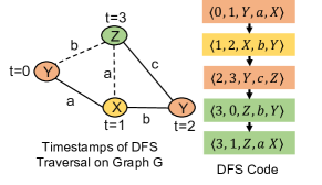
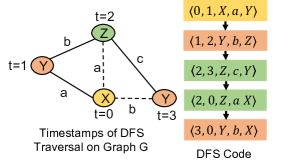
Now, we introduce minimum DFS codes and how it corresponds to canonical labels of graphs. DFS code [23] is a mapping function defined over a graph $G$, which encodes $G$ into a sequence of edge tuples. To construct a DFS-code from $G$, first, a depth-first search (DFS) traversal is started from an arbitrary node. During this traversal, a timestamp is assigned to each node based upon when it is discovered. The first discovered node is assigned timestamp $0$, the second discovered node is assigned $1$, and so on. Following these timestamps, each edge $(u,v)$ is assigned a tuple of five items $\left\langle t_{u},t_{v},L_{u}=\mathbb{L}_{node}(u),L_{uv}=\mathbb{L}_{edge}(uv),L_{v}=\mathbb{L}_{node}(v)\right\rangle$. $t_{u},\;t_{v}$ are the discovery times of node $u$ and $v$ respectively. $L_{u},\;L_{v}$ and $L_{uv}$ are labels of node $u$, node $v$ and edge $(u,v)$ respectively.

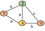
A partition of edges is created based upon the DFS traversal. The first partition consists of forward edges that are traversed by the DFS traversal. The second partition contains backward edges, that are not traversed during the DFS traversal. For example, in Fig.  3b, 3c, the edges depicted by solid lines depict the forward edges, and the one’s which are dashed depict backward edges. A total ordering is imposed on these edges following the rules described in gSpan [23] to obtain the DFS code of a graph. Specifically, for ordering forward edges, the process is straight forward. Forward edges are ordered based upon their discovery time in the DFS traversal. For backward edges, the ordering is derived based upon the following rules:

• Backward edge $(u,s)$ must appear before all forward edges of the form $(u,t)$.

• Backward edge $(u,s)$ must appear after the forward edges of the form $(t,u)$, i.e the first forward edge which points to $u$.

• For backward edges of the form $(u,s)$ and $(u,s^{\prime})$ originating from the same source $u$, $(u,s)$ is ordered before $(u,s^{\prime})$ if $t_{s}<t_{s}^{\prime}$.

Fig. 3 shows examples of two DFS codes of a graph based on two DFS traversals. For more details on DFS code, we refer to GSpan[23].

Minimum DFS codes: As shown in Fig.3, a graph can have multiple DFS codes. We choose the lexicographically smallest DFS code among all DFS codes as the minimum DFS code. It has been shown that there exists a bijection between a graph and its minimum DFS code [23]. Hence, minimum DFS codes are canonical labels. Using minimum DFS codes, we encode each graph $G=(V,E)$ in dataset $D$ as a sequence of $m$ edge tuples $S=(s_{1},\ldots,s_{m})$ where $m=|E|$ and each $s_{i}$ is an edge tuple of the form $\left\langle t_{u},t_{v},L_{u},L_{uv},L_{v}\right\rangle$. We use the notation $\mathcal{F}(G)=S$ to denote the minimum DFS code $S$ of graph $G$. Applying $\mathcal{F}$ on all graphs of dataset $D$, we obtain a collection of edge tuple sequences $\mathcal{S}=\left\{\mathcal{F}(G)\mid\forall G\in D\right\}$ for all graphs in dataset $D$.

Computation Complexity: We note that computing the minimum DFS code of a graph is equivalent to performing graph isomorphism tests. In the literature, no polynomial time algorithm exists for detecting graph isomorphism. Fortunately, for labeled graphs, it has been shown that minimum DFS codes can be computed very efficiently[23, 2].

3.3 Modeling Graph Sequences

Minimum DFS codes are of sequential nature. We model each sequence $S{=}(s_{1},\cdots,s_{m})$ using an auto-regressive model[2] as follows:

$$\vspace{-0.04in}p(S)=p(s_{0})\prod_{i=1}^{m+1}p(s_{i}|s_{0},\cdots,s_{i-1})$$ (1)

where $m{=}{{\mid}{E}{\mid}}$ is the number of edges, $s_{0}$ is a start-of-sequence SOS token and $s_{m+1}$ is end-of-sequence EOS token to allow variable length sequences. To learn the parameters for these sequential conditional distributions, we use Recurrent Neural Networks. Specifically, we use LSTM [24], which efficiently models long-range dependencies. Formally,

$$\vspace{-0.05in}\mathbf{h}_{i} =LSTM^{hidden}_{\theta}\left(\mathbf{h}_{0},\left(f^{emb}_{\theta}(s_{0})\ldots f^{emb}_{\theta}(s_{i-1})\right)\right) =LSTM^{hidden}_{\theta}\left(\mathbf{h}_{i-1},f^{emb}_{\theta}\left(s_{i-1}\right)\right)$$ (2)

where $LSTM_{\theta}$ is a function representing an LSTM cell. $f^{emb}_{\theta}$ is an embedding function that takes one-hot encoding of $s_{i-1}$ as input and produces a $d$-dimensional compressed vector. $\mathbf{h}_{0}$ is initialized to $\bm{0}$. Finally, assuming that $s_{i}.t_{u}$, $s_{i}.t_{v}$, $s_{i}.L_{u}$, $s_{i}.L_{uv}$, $s_{i}.L_{v}$ are independent given $\mathbf{h}_{i}$, we predict $s_{i}=\langle t_{u},t_{v},L_{u},L_{uv},L_{v}\rangle$ as follows.

$$\widetilde{s_{i}}=\left\langle f^{t_{u}}_{\theta}(\mathbf{h}_{i}),f^{t_{v}}_{\theta}(\mathbf{h}_{i}),f^{L_{u}}_{\theta}(\mathbf{h}_{i}),f^{L_{uv}}_{\theta}(\mathbf{h}_{i}),f^{L_{v}}_{\theta}(\mathbf{h}_{i})\right\rangle$$ (3)

where each $f_{\theta}$ is a function representing a fully connected Multi-layered Perceptron (MLP). Note that every function in this discussion is parameterized by $\theta$ (indicated by the subscript). Finally, we define the loss $\mathcal{L}_{D}$ specific to sequence (graph) generation task $\mathcal{T}_{D}$ on dataset $D$ as follows:

$$\mathcal{L}_{S}=-\sum_{i=1}^{m+1}\sum_{c}\left(s_{i}[c]\log\widetilde{s}_{i}[c]+\left(1-s_{i}[c]\right)\log\left(1-\widetilde{s}_{i}[c]\right)\right) \quad\text{,}\quad\mathcal{L}_{D}=\sum_{S\in\mathcal{S}}\mathcal{L}_{S}$$ (4)

Here $c$ is the component index of one-hot vector $s_{i}$ and predicted vector $\widetilde{s}_{i}$. $\mathcal{S}$ is the collection of graph sequences $S$ derived by encoding every graph $G{\in}D$ using minimum DFS coding function $\mathcal{F}(G)$.

3.4 Meta-Learning for Labeled Graph Generative Modeling under limited availabiltiy of data

Up until now, we have defined parameters $\theta$ of graph generative model $p_{\theta}(D)$. As motivated, we want to find an initialization of $\theta$ such that it can quickly learn to generate graphs from unseen dataset $D_{T}$ having small number of training graph samples. Specifically, we train $\theta$ on graphs from auxiliary datasets to learn initial parameters. To do this, we build upon the Reptile framework [25]. Reptile is a first-order meta-learning algorithm, wherein it uses first-order gradients to learn $\theta$, and is therefore computationally and memory efficient. GShot, using Reptile, extracts the meta-knowledge to obtain an effective initialization and an ability to adapt to the target dataset using limited fine-tuning samples. More concretely, GShot optimizes the below objective function in order to learn good initialization of $\theta$:

$$\min_{\theta}\,\mathbb{E}_{{\mathcal{L}_{D\sim\mathcal{D}}}}\left[\mathcal{L}_{D}(\theta_{D}^{K})\right],\vspace{-0.1in}$$ (5)

where $\theta_{D}^{K}$ are the updated parameters after $K$ gradient updates of $\theta$ from dataset ${D}$ as follows:

$$\theta^{0}=\theta \quad\text{and}\quad\quad\theta_{D}^{i}=\theta_{D}^{i-1}-\alpha\nabla_{\theta^{i-1}}\mathcal{L}_{D}\;\;\;\forall i\in[1\ldots K]$$ (6)

Here hyper-parameter $\alpha$ controls the meta-learning rate. Finally using the $K$ step updated parameters $\theta^{K}_{D}$, we optimize Eq. 5 as follows:

$$\theta=\theta+\epsilon\left(\theta^{K}_{D}-\theta\right)$$ (7)

where $\epsilon$ and $K$ are hyper-parameters of GShot. Eq. 7 updates the value of the meta-parameters $\theta$ using a weighted combination of $\theta$ and K-step fine-tuned parameter $\theta^{K}_{D}$ for dataset $D$. The parameter $\epsilon$ can be considered as a step-size in the direction of the gradient $\theta^{K}_{D}-\theta$. We iterate over $D{\sim}\mathcal{D}$ by computing Eq. 6 for different tasks and then using it for optimizing Eq. 5. Algorithm  1 in App. describes the pseudocode of meta-training procedure of GShot.

3.5 Adaptation to Target Dataset

Once GShot is meta-trained on diverse graph datasets, our next goal is to adapt the learned model parameters to the target dataset ${D_{T}}$. Essentially, first we initialize the target model parameters to the value of the meta-trained model:

$$\theta_{T}=\theta$$ (Initialization)

Towards our goal to optimize parameters on the target dataset, a simple approach is to update the parameters of the model by applying multiple gradient updates using samples from target dataset $D_{T}$ with its associated loss as follows:

$$\vspace{-0.1in}\theta_{T}=\; \theta_{T}-\alpha\nabla_{\theta_{T}}\mathcal{L}_{T}$$ (gradient updates)

The above equation assumes, for every gradient update, the training data is sampled in a random fashion from the target dataset. However, recent studies have discovered that gradually increasing the complexity of training instances results in better learning and faster convergence [26]. Motivated by this result, we adopt self-paced learning [27] in the fine-tuning phase of GShot. Towards this end, we modify the loss $\mathcal{L}_{T}$ associated with the target dataset in a way that the model is presented with training samples of gradually increasing difficulty. Moreover, the training curriculum is dynamically determined by the model itself based upon its perception of the difficulty of a sample. Specifically, recall from Eq. 4 $\mathcal{L}_{D}=\sum_{S\in\mathcal{S}}\mathcal{L}_{S}$ where $\mathcal{S}$ is the collection of graph sequences of $G\in D$. For self-paced learning, we modify $\mathcal{L}_{T}$ as follows:

$$\mathcal{L}_{T} =\sum_{i=1}^{\mid\mathcal{S}_{T}\mid}\beta_{i}\mathcal{L}_{S_{i}}-\lambda\sum_{i=1}^{\mid\mathcal{S}_{T}\mid}\beta_{i} \quad\quad\beta_{i}\in \{0,1\}\;\;\forall i\in[1\ldots{\mid}\mathcal{S}_{T}{\mid}]$$ (8)

where $\mathcal{S}_{T}{=}\{\mathcal{F}(G)\mid\forall G\in D_{T}\}$, $S_{i}{\in}\mathcal{S}_{T}$, and ${{\mid}{\mathcal{S}_{T}}{\mid}}$ is the number of graphs in $D_{T}$. $\lambda$ is an evolving parameter that essentially controls the pace of learning. Specifically in our graph generative modeling setting, we solve this via an iterative approach [27]. Before every gradient update as described earlier, we first calculate the value of $\beta_{i}$’s as follows:

$$\beta_{i}=\begin{cases}1&if\;\;\mathcal{L}_{S_{i}}<\lambda\\ 0&else\end{cases}$$ (9)

The value of $\beta_{i}$ indicates whether the $i^{th}$ training sample will be used or not in the loss computation in Eq. 8 . We substitute these values in Eq. 8 and update the parameters $\theta_{T}$. This process repeats until convergence. The value of $\lambda$, is increased periodically by a growth factor $\gamma$ to gradually allow hard samples to be a part of the loss computation during the course of training. Algorithm  2 in App. describes the pseudocode of the fine-tuning procedure of GShot.

3.6 Graph Generation

After fine tuning $p_{\theta}(D)$ on target dataset $D_{T}$, we obtain $p_{\theta_{T}}(D_{T})$. We sample graphs from this distribution as follows. First, we pass the initial hidden state $\mathbf{h}_{0}{=}\bm{0}$ to $LSTM_{\theta_{T}}$ along with the SOS symbol. At each step $i$, we sample $s_{i}$ from the updated hidden state $\mathbf{h}_{i}$ as follows-

$$s_{i}.t_{u} \sim\;Multinomial(f^{t_{u}}_{\theta_{T}}(\mathbf{h}_{i})) \quad s_{i}.t_{v} \sim\;Multinomial(f^{t_{v}}_{\theta_{T}}(\mathbf{h}_{i}))$$

$$s_{i}.L_{u} \sim\;Multinomial(f^{L_{u}}_{\theta_{T}}(\mathbf{h}_{i})) \quad s_{i}.L_{uv} \sim\;Multinomial(f^{L_{uv}}_{\theta_{T}}(\mathbf{h}_{i}))$$ (10)

$$s_{i}.L_{v} \sim\;Multinomial(f^{L_{v}}_{\theta_{T}}(\mathbf{h}_{i}))$$ (11)

The process is repeated until the EOS symbol is sampled for any of the five components in the sampled tuple. Finally, this sampled sequence, representing the DFS code, is converted back to graph. Algorithm 3 in App. presents the pseudocode of the graph generation phase.

4 Experiments

We benchmark GShot against state-of-the-art algorithms for graph generation and establish that:

• Higher fidelity: GShot generates graphs of higher fidelity than the state-of-the-art methods.

• Sample-efficient: Attributed to its capability to learn with a limited amount of data, GShot better preserves graph properties compared to existing methods even when the number of fine-tuning samples used by GShot are relatively less compared to other methods.

The code to reproduce the experiments can be found at https://github.com/idea-iitd/GShot.

4.1 Experimental setup

Datasets: Since our focus is on domain-agnostic labeled graph generative modeling, we show the effectiveness of our proposed approach using datasets from diverse domains. Moreover, in our experiments, we use target datasets having significantly low volumes of available graphs in comparison to other works in literature [2, 13, 28, 6]. Table  3 in App.  C summaries the different datasets. Further details on semantics of the datasets are also present in App. C.

Train-test splits: We briefly describe our datasets’ train-test split.

• Biological Domain: Each enzyme in the Enzyme dataset[11] belongs to one of six classes, namely EC1, EC2, EC3, EC4, EC5, EC6. We treat enzymes in EC1, EC2, EC4, EC5, EC6 as auxiliary datasets and EC3 as our target dataset, which consists of $100$ enzymes.

• Chemical Domain: We use anti-cancer screen datasets Yeast, Breast, and Lung as auxiliary datasets for meta-training and use the two smallest chemical datasets of AIDS-CA and Leukemia-Active as our target set.

• Physics Domain: We meta-train GShot on auxiliary datasets consisting of four and six particle spring systems and then fine-tune on graphs containing five particles.

Baselines:We benchmark the performance of GShot against the state-of-the-art techniques for domain-agnostic, labeled graph generative modeling, namely GraphGen [2] and GraphRNN [13]. We do not include GRAN[6] as a baseline since it cannot generate labeled graphs. For GraphGen, we used the code shared by authors. While, in theory, GraphRNN supports labeled graphs, the code shared by the authors do not. Hence, we extend the author’s code as outlined in the supplementary section of GraphRNN [13]. Both GraphGen and GraphRNN are trained only on the target dataset and we compare the quality of the generated graphs with that of GShot. This comparison allows us to evaluate how efficient the knowledge transfer of GShot is as opposed to relying only on the target dataset.

In addition, we use a third pre-training baseline introduced by us, which we will refer to as PreTrain+FT. In this baseline, we first pre-train GraphGen on the same auxiliary datasets used by GShot for meta-training. Then, we fine-tune it on the target dataset. This baseline allows us to systematically understand the impact of meta-learning against generic generative modeling. We do not consider pre-training on GraphRNN, since GraphGen has been shown to be superior on the labeled graph generative modeling task [2], which is also reflected in our experiments that follows.

Evaluation setup: During meta-training of GShot, we use ${\approx}50\%$ data for training and the same for validation. During fine-tuning to a new graph dataset, unless specifically mentioned, we use the default split among training, validation, and test as ${\approx}40\%$, ${\approx}30\%$, and ${\approx}30\%$ respectively. Unless specified otherwise, for training a model from scratch directly on the target dataset or fine-tuning a model on a target dataset, we use the same number of training samples of the target dataset. For each target dataset, this information is present in the #Target Training samples column of Table  4.1. The system configuration and parameter details can be found in App. D.

Evaluation Metrics: The performance of a graph generative model is satisfactory (1) if it generates graphs with similar properties as the source graphs, (2) but without duplicating the source graphs themselves. To quantify these, we divide our metrics into two categories.

• Fidelity: To quantify the preservation of graph properties, we compare the distributions of graph statistics between the ground truth graphs and the generated graphs using the following metrics.

  • Structural metrics: To quantify the preservation of original graph properties, we use the structural metrics used by GraphRNN and GraphGen: (1) node degree distribution (Degree), (2) clustering coefficient distribution of nodes (Clustering), and (3) orbit count distribution (Orbit) [29], which measures the number of orbits with $4$ nodes. This metric captures the higher-level motifs that are shared between generated and test graphs. We utilize Maximum Mean Discrepancy (MMD) [30] to compute the distance between two distributions. Further, to compare the sizes of the generated graphs against the ground truth, we measure (4) Average node count and (5) Average edge count.

  • Labeled Graph Metrics: Our work is geared towards labeled graph generation. Hence, it is important to assess whether a generative model captures the label distribution well. Towards that end, we compare the distribution of (1) Node Labels, (2) Edge Labels, and (3) the joint distribution of node labels and degree in the ground truth and generated graphs. We again use MMD to quantify the distance from the ground truth.

  • Topological Similarity: Finally, in order to capture topological similarity of generated graphs with the ground truth graphs, we use Neighbourhood Sub-graph Pairwise Distance Kernel (NSPDK) [31]. NSPDK provides the benefit of incorporating both node and edge labels along with the structure of the graph. Specifically, NSPDK measures the distance between two graphs by matching pairs of subgraphs with different radii and distances. The lower the MMD score for NSPDK, the more aligned are the two graph distributions.

• Duplication and Uniqueness: A model that generates graphs with high fidelity might not be useful in practice unless it is also capable of generating graphs that are not seen in the training data. In order to capture this requirement, we utilize the below metrics introduced by GraphGen [2]: (1) Novelty measures the percentage of generated graphs that are not subgraphs of the set of the training graphs. Additionally, we compute (2) Uniqueness, which captures the diversity of the set of generated graphs. In order to quantify uniqueness, we remove the generated graphs that are subgraph isomorphic to any of the other generated graphs. This is different from the novelty metric as here we focus only on the generated graphs. A model that generates $100$ graphs and out of which $90$ are subgraph isomorphic to any of the other generated graphs has uniqueness${=}10\%$.

In order to quantify the quality of a particular metric, we generate multiple graphs for each target dataset and compare them against the available ground truth target graphs. Details of number of graphs generated for each dataset is present in App. D.2.

Table 1: Summary of performance by GShot, GraphGen, GraphRNN, and PreTrain+FT baseline on different datasets on multiple metrics. Values less than $10^{-3}$ are approximated to 0. The best-performing model for each dataset is highlighted in bold.

Auxiliary datasets	Target dataset	#Target Training Samples	Model	Deg.	Clus.	Orbit	NSPDK	Avg # Nodes (Gen/Gold)	Avg # Edges (Gen/Gold)	Node Label	Edge Label	Joint Node Label & Degree	Novelty	Uniqueness
Enzyme: EC1,EC2, EC4,EC5, EC6	Enzyme: EC3	50	GraphGen	0.90	0.58	0.127	0.266	17.51/26.90	22.22/52.85	0.015	x	0.714	100%	100%
			GraphRNN	0.30	0.73	0.13	0.214	20.51/26.90	36.23/52.85	0.019	x	0.696	100%	100%
			PreTrain+FT	0.72	0.63	0.053	0.18	23.73/26.90	33.2/52.85	0.0095	x	0.619	$99\%$	$99\%$
			GShot	0.45	0.47	0.025	0.16	24.5/26.90	37.69/52.85	0.004	x	0.457	100%	100%
Yeast, Breast, Lung	AIDS-CA	150	GraphGen	0.026	$0.016$	$0.003$	0.127	17.51/37.14	17.62/39.60	0.05	$0.001$	0.20	$98\%$	$97\%$
			GraphRNN	0.15	0.47	0.045	0.14	30.5/37.14	40.19/39.60	0.193	0.005	0.836	$86\%$	$45\%$
			PreTrain+FT	0.021	0.004	$\approx 0$	0.11	24.1/37.14	25.22/39.60	0.013	$\approx$ 0	0.173	99%	99%
			GShot	0.017	0.0015	$\approx$ 0	0.08	26.5/37.14	27.1/39.60	0.011	$\approx$ 0	0.14	99%	99%
	Leukemia-Active	500	GraphGen	0.06	$0.019$	$\approx 0$	0.17	40.02/47.71	42.23/50.37	0.02	$\approx$ 0	0.99	100%	100%
			GraphRNN	0.06	0.554	0.032	0.34	7.17/47.71	7.51/50.37	0.39	0.017	0.83	100%	100%
			PreTrain+FT	0.039	0.0064	$\approx$ 0	0.116	43.08/47.71	45.5/50.37	0.09	$\approx$ 0	0.79	$98\%$	$98\%$
			GShot	0.0069	$\approx$ 0	$\approx$ 0	0.032	42.35/47.71	44.33/50.37	0.0011	$\approx$ 0	0.24	100%	100%
{4, 6} body Spring	5-body Spring	500	GraphGen	0.004	0.015	$\approx$ 0	0.016	4.98/5	5.49/5.64	0.012	x	0.011	33%	13%
			GraphRNN	0.018	0.012	$\approx$ 0	0.029	4.71/5	5.03/5.64	0.044	x	0.017	87%	55%
			PreTrain+FT	0.021	0.047	0.0025	0.017	4.98/5	5.19/5.64	0.011	x	0.012	$70\%$	$49\%$
			GShot	0.008	0.035	$\approx$ 0	0.016	4.98/5	5.38/5.64	0.016	x	0.012	64%	41%

4.2 Quality

Fidelity: Table 4.1 shows the performance of all the models across different datasets. We observe that, in most cases, GShot obtains lower MMD scores compared to baselines. In terms of the global level graph metric NSPDK, GShot achieves a significant improvement even against the best performing baselines. For instance in Leukemia-Active, for NSPDK, GShot obtains MMD value of $0.032$ against a significantly higher value of $0.116$ obtained by PreTrain+FT. With respect to labeled graph metrics, we observe that GShot improves over state-of-the-art techniques by achieving more than $50\%$ lower MMD value in multiple cases. Further, GShot also outperforms existing techniques in the Joint Node-Label and Degree metric signifying its ability to better jointly model the graph structure and labels. While GShot achieves high quality on most fidelity metrics, however on the node/edge count metric when the number of fine-tuning graphs becomes very low(Eg:- Enzyme EC3 = 50 and AIDS-CA = 150), its performance deteriorates for this metric. We would also like to highlight that modeling the edge tuple conditionally in GShot (see App  G), improves this metric to a certain extent on all datasets. Among all baselines only GraphRNN’s performance on AIDS-CA for avg node/edge count is superior to GShot, however it performs worser on other fidelity metrics . Having said that, the superior performance of GShot establishes the efficacy of the meta-training procedure to learn an effective set of initial model parameters, which adapts well to low-data regimes.

Uniqueness and novelty: In addition to obtaining better fidelity in most cases, GShot also achieves a higher or similar score compared to baselines on the Novelty and Uniqueness aspect. On AIDS-CA dataset, we obtain an improvement of ${\approx}1{-}2\%$ in the uniqueness and novelty metrics against GraphGen while also achieving better fidelity scores. Additionally, for AIDS-CA, GraphRNN’s performance in terms of both fidelity as well as diversity is significantly inferior to other methods. In the case of the $5$-body spring dataset, although GShot does not perform the best in terms of fidelity scores, still its uniqueness and novelty scores are significantly higher than GraphGen, which achieves a $33\%$ novelty score and $13\%$ uniqueness score. This indicates that GraphGen mostly generated duplicated graphs. In context of Physics dataset, we highlight that the target graphs are extremely small i.e having only 5 nodes. It is more challenging to generate unique and diverse graphs in this context when compared to datasets belonging to other category such as chemical/biological where graphs are large. We observe that only GraphRNN is able to generate graphs which are more novel and unique, however, its performance is significantly poor on all fidelity metrics. Overall, we observe that an efficient parameter initialization obtained by GShot also helps in improving the diversity of generated graphs while generating graphs with high fidelity.

Figure 4: The variation in MMD scores on different metrics when the number of fine-tuning samples for GShot is reduced from $500$ to $50$ on the Leukemia-Active dataset. Here the suffix of $500$ after GraphGen and PreTrain+FT depicts that the number of training samples used from the target dataset for these baselines is $500$. Note that for PreTrain+FT 500, the value of the Node-Label metric ($0.09$) was skipped in the diagram to improve readability.

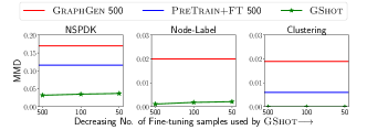
Robustness to number of fine-tuning samples: We also evaluate GShot’s robustness to different sizes of the same fine-tuning dataset. Towards this end, we choose Leukemia-Active dataset as our target dataset since due to slightly higher availability of fine-tuning data, there is a reasonable scope to down-sample the fine-tuning data in order to understand its impact on performance. We vary the number of fine-tuning samples available to GShot from $500$ to $50$. However, we keep the number of fine-tuning samples for the baselines to the maximum value, i.e., $500$. In Fig. 4, we observe that GShot, while using less number of samples from the target dataset, still obtains lower MMD scores on different metrics in comparison to GraphGen and the PreTrain+FT model that used $500$ samples from the target dataset. Further, the MMD scores for GShot increase only slightly when the number of fine-tuning samples is reduced from $500$ to $50$. This is a direct consequence of our model’s ability to adapt with a small number of training samples. Further, we would like to highlight that the novelty and uniqueness metrics did not show any observable change in this experiment.

Ablation study: We study the improvement obtained by using self-paced fine-tuning in GShot over vanilla fine-tuning in Appendix E. In Appendix  F, we study the impact of the choice of auxiliary datasets on the performance of graph generative modeling under data scarcity.

5 Conclusion

Research on deep graph generative modeling has progressed significantly in several directions such as scalability to large graphs, domain agnostic modeling, handling node and edge labels, etc. However, the problem of learning to generate graphs in low-data regimes remained unexplored. In this work, we propose the paradigm of domain-agnostic, labeled graph generative modeling under data scarcity. Our proposed architecture GShot learns to transfer meta-knowledge from auxiliary graph datasets to a target dataset. Utilizing these prior experiences, GShot quickly adapts to an unseen graph dataset through self-paced fine-tuning. GShot is effective in learning graph distributions on datasets with small number of available training samples. Extensive evaluation on real graph datasets demonstrate that graphs generated by GShot preserve graph structural properties significantly better than the state-of-the-art approaches. Although, our proposed method outperforms existing state-of-the-art methods, however, while generating these molecules, it does not take into account their molecular/chemical properties etc. In future, we would like to work on capturing these aspects.

6 Acknowledgement

Srikanta Bedathur was partially supported by a DS Chair of AI fellowship. Sayan Ranu acknowledges the Nick McKeown chair position endowment. Sahil Manchanda was partially supported by Qualcomm Innovation Fellowship.

7 Appendix

Appendix A Notations

Symbol	Meaning
$G=(V,E)$	A Graph with vertex set $V$ and edge set $E$
$n$	Number of nodes in $G$
$m$	Number of edges in $G$
$\mathbb{V}$	Label set of vertices in $G$
$\mathbb{E}$	Label set of edges in $G$
$D{=}\{G_{1},G_{2},\cdots,G_{N}\}$	Dataset of $N$ graphs
$\mathcal{D}{=}\{D_{1},\cdots,D_{\mathcal{B}}\}$	Collection of $\mathcal{B}$ graph datasets
$t_{u}$	DFS discovery time of node $u$
$t_{v}$	DFS discovery time of node $v$
$L_{u}$	Label of node $u$
$L_{uv}$	Label of edge $(u,v)$
$L_{v}$	Label of node $v$
$\mathcal{F(G)}$	Function to map graph to Minimum DFS code $S$
$S=(s_{1},s_{2}\ldots s_{m})$	Minimum DFS Codes of a graph
$\mathcal{S}=\{S_{1},S_{2}\cdots S_{N}\}$	Collection of Minimum DFS codes of a dataset with $N$ graphs
$\mathcal{T}$	Set of graph generative modelling tasks
$\mathcal{T}_{i}$	Graph generative modelling task for the $i^{th}$ dataset
$\mathcal{L}_{i}$	Loss associated with dataset $D_{i}$
$\theta$	Model parameters
$D_{T}$	Target graph dataset
$\mathcal{S}_{T}$	Collection of Minimum DFS codes for target dataset $D_{T}$
$\theta_{T}$	Parameters fine-tuned to the dataset $D_{T}$
$\beta_{i}$	Binary loss coefficient for $i^{th}$ sample in eq. 8
$\gamma$	Growth parameter in self-paced fine-tuning

Table 2: Notations used in the paper

Appendix B Pseudocodes

Input : Collection of $\mathcal{B}$ graph datasets $\mathcal{D}=\{D_{1},D_{2}\ldots D_{\mathcal{B}}\}$, $K$, $\epsilon$

Output : Good initialization of parameters $\theta$ of generative model $p_{\theta}(D)$

Initialise meta-parameters $\theta$ randomly.

repeat

       Sample a dataset $D\in\mathcal{D}$

      

      $\mathcal{S}=\{S=\mathcal{F}(G)\>|\>\forall G\in D\}$

        // Get Minimum DFS code

       $\theta_{D}\leftarrow\theta$

        // Dataset $D$ specific parameters

       for $K$ times do // $K$ inner gradient steps

             $S=[s_{1},s_{2}\ldots s_{m}]\sim\mathcal{S}$

             $s_{0}$ $\leftarrow$ SOS

            

            $h_{0}$ $\leftarrow$ $\bm{0}$

             $\mathcal{L}_{D}\leftarrow 0$

             /* Computing loss $\mathcal{L}_{D}$ of sequence $S=[s_{0},s_{1},s_{2}\ldots s_{m+1}]$ */

             for  $i$ from $1$ to $m+1$ do // $s_{m+1}$ for EOS tokens

                   $\mathbf{h}_{i}\leftarrow LSTM^{hidden}_{\theta}(\mathbf{h}_{i-1},f^{emb}_{\theta}(s_{i-1}))$

                  

                  $\widetilde{s}_{i}\leftarrow\left\langle f^{t_{u}}_{\theta}(\mathbf{h}_{i}),f^{t_{v}}_{\theta}(\mathbf{h}_{i}),f^{L_{u}}_{\theta}(\mathbf{h}_{i}),f^{L_{uv}}_{\theta}(\mathbf{h}_{i}),f^{L_{v}}_{\theta}(\mathbf{h}_{i})\right\rangle$

                  

                  $\mathcal{L}_{D}\leftarrow\mathcal{L}_{D}+\sum_{c}\left(s_{i}[c]\log\widetilde{s}_{i}[c]+\left(1-s_{i}[c]\right)\log\left(1-\widetilde{s}_{i}[c]\right)\right)$

                  

            $\theta_{D}\leftarrow\theta_{D}-\alpha\nabla_{\theta_{D}}\mathcal{L}_{D}$

              // D specific parameters’ update

            

      Update $\theta\leftarrow\theta+\epsilon(\theta_{D}-\theta)$

        // Meta gradient update

      

until stopping criteria

// Typically when validation loss is minimized

Algorithm 1 Pseudocode for meta-training phase of GShot

Input : Target dataset $D_{T}$, meta-trained parameters $\theta$, batch size $B$, growth factor $\gamma$, $\lambda$

Output : Fine tuned parameters $\theta_{T}$ for target dataset $D_{T}$

$\mathcal{S_{T}}=\{S=\mathcal{F}(G)\>|\>\forall G\in D_{T}\}$

  // Get Minimum DFS code

$\theta_{T}\leftarrow\theta$

  // Initializing parameters specific to target dataset $D_{T}$

repeat

       $\mathcal{L}_{T}\leftarrow 0$;

      for $B$ times do // Sample $B$ graphs for every batch

             $S=[s_{1},s_{2}\ldots s_{m}]\sim\mathcal{S_{T}}$

             $s_{0}$ $\leftarrow$ SOS

            

            $h_{0}$ $\leftarrow$ $\bm{0}$

            

            $l\leftarrow 0$

              // Instance specific loss

             /* Computing loss $l$ of sequence $S=[s_{0},s_{1},s_{2}\ldots s_{m+1}]$ */

             for  $i$ from $1$ to $m+1$ do // $s_{m+1}$ for EOS tokens

                   $\mathbf{h}_{i}\leftarrow LSTM^{hidden}_{\theta_{T}}(\mathbf{h}_{i-1},f^{emb}_{\theta_{T}}(s_{i-1}))$

                  

                  $\widetilde{s}_{i}\leftarrow(f^{t_{u}}_{\theta_{T}}(\mathbf{h}_{i}),f^{t_{v}}_{\theta_{T}}(\mathbf{h}_{i}),f^{L_{u}}_{\theta_{T}}(\mathbf{h}_{i}),f^{L_{uv}}_{\theta_{T}}(\mathbf{h}_{i}),f^{L_{v}}_{\theta_{T}}(\mathbf{h}_{i}))$

                  

                  $l\leftarrow l+\sum_{c}\left(s_{i}[c]\log\widetilde{s}_{i}[c]+\left(1-s_{i}[c]\right)\log\left(1-\widetilde{s}_{i}[c]\right)\right)$

                  

            if $l<\lambda$ then

                   $\mathcal{L}_{T}=\mathcal{L}_{T}+l$

                  

            

      $\theta_{T}\leftarrow\theta_{T}-\alpha\nabla_{\theta_{T}}\mathcal{L}_{T}$

      

      $\lambda=\lambda*\gamma$

        // Increase difficulty periodically

      

until stopping criteria

// Typically when validation loss is minimized

Algorithm 2 Fine-tuning GShot on target dataset $D_{T}$

Input : Fine tuned parameters $\theta_{T}$ of deep generative model $p_{\theta_{T}}$

Output : Graph $G$

$S\leftarrow\left(\right)$

$s_{0}\leftarrow SOS$

$i\leftarrow 0$

$\mathbf{h}_{0}\leftarrow\bm{0}$

repeat

       $i\leftarrow i+1$

       $\mathbf{h}_{i}\leftarrow LSTM^{hidden}_{\theta_{T}}(\mathbf{h}_{i-1},f^{emb}_{\theta_{T}}(s_{i-1}))$

       // Sample $s_{i}$ from multinomial distributions parameterized using $\mathbf{h}_{i}$

       $s_{i}.t_{u}\sim Multinomial(f^{t_{u}}_{\theta_{T}}(\mathbf{h}_{i}))$

       $s_{i}.t_{v}\sim Multinomial(f^{t_{v}}_{\theta_{T}}(\mathbf{h}_{i}))$

       $s_{i}.L_{u}\sim Multinomial(f^{L_{u}}_{\theta_{T}}(\mathbf{h}_{i}))$

       $s_{i}.L_{uv}\sim Multinomial(f^{L_{uv}}_{\theta_{T}}(\mathbf{h}_{i}))$

       $s_{i}.L_{v}\sim Multinomial(f^{L_{v}}_{\theta_{T}}(\mathbf{h}_{i}))$

       $S.append(s_{i})$

      

until EOS $\in\{s_{i}.t_{u},s_{i}.t_{v},s_{i}.L_{u},s_{i}.L_{uv},s_{i}.L_{v}$}

// Check if any item of tuple $s_{i}$ contains $EOS$ symbol $G\leftarrow{\mathcal{F}}^{-1}(S)$

  // Convert DFScode back to graph

return $G$

Algorithm 3 Pseudocode of graph generation for target dataset $D_{T}$

Appendix C Dataset Semantics

Biological Domain: Proteins are biomolecules consisting of long chain of amino acids. They are highly essential to our lives and significantly interesting in certain biomedical tasks such as de novo protein design[32, 33]. Enzymes, a set of specialized proteins, are catalysts that can speed up metabolic activities. In our work, we utilize the Enzyme dataset from the BRENDA enzyme database [34], which consists of protein tertiary structures. We convert enzymes to graphs where nodes represent secondary structures labeled into one of the three categories namely helices, turns, or sheets. This dataset does not have edge labels. The dataset is divided into six classes and each enzyme belongs to one of these classes, namely EC1, EC2, EC3, EC4, EC5, EC6. For our limited data learning setup, we consider learning to generate graphs belonging to a certain enzyme class as a task. We treat the datasets EC1, EC2, EC4, EC5, EC6 as auxiliary and EC3 as our target dataset, which consists of $100$ enzymes.

Chemical Domain: Chemical compounds are composed of two or more atoms connected using chemical bonds. We utilize the following chemical compounds datasets to train and evaluate GShot.

AIDS-CA [23]: This dataset comprises of a set of molecules that displayed activity against HIV.

Breast, Lung, Yeast: Each of these three datasets contain molecules that were screened for activity against Breast cancer, Lung cancer and cancer in Yeast respectively [12].

Leukemia-Active: This dataset consists of compounds that are active against Leukemia [12].

In all chemical datasets, we convert compounds to labeled graphs where nodes represent atoms and their labels represent atom-type which are elements belonging to the chemical periodic table. Edges in the graphs represent bonds and edge labels encode the bond type i.e single, double, triple.

For the limited data learning setup for chemical domain, Yeast, Breast, and Lung are used as auxiliary datasets during meta-training. Further, we choose AIDS-CA and Leukemia-Active datasets as our target datasets. The reasons for this choice is (1) due to their relatively low availability of number of graph samples and (2) since they consist of compounds that are active against certain diseases, therefore have more practical utility.

Physics Domain: Physics-based simulations are commonly used to understand interactions among different objects[19, 18, 17]. Dynamical systems such as $N$-body springs can be converted into graph structures where nodes represent particles and edges represent connections between particles. We utilize the dataset of the $N$-body spring simulations [19]. It consists of $N$ particles in a two-dimensional space partitioned into a $5{\times}5$ grid . Two particles are connected to each other via spring with a probability of $0.5$. The label of a node is the partition it lies in. This system does not have edge labels[19]. For learning under limited data, we meta-train GShot on auxiliary datasets consisting of four and six particle systems and then fine-tune on graphs containing five particles.

Table 3: Summary of the datasets

#	Name	Domain	No. of graphs	$|V|$	$|E|$	$|\mathbb{V}|$	$|\mathbb{E}|$
1	Enzymes[11]	Biological	600	[2, 125]	[2, 149]	3	X
2	NCI-H23 (Lung)[12]	Chemical	24k	[6, 50]	[6, 57]	11	3
5	Yeast[12]	Chemical	47k	[5, 50]	[5, 57]	11	3
7	MCF-7 (Breast)[12]	Chemical	23k	[6, 111]	[6, 116]	11	3
6	Leukemia-Active[12]	Chemical	1900	[12, 107]	[12, 111]	11	3
6	AIDS-CA[12]	Chemical	328	[10, 189]	[10, 196]	11	3
8	N-body Spring[19]	Physics	1500	N	[3, 13]	25	X

Appendix D Experimental Setup and Reproducibility

All experiments are performed on a machine with Intel Xeon Gold 6284 processor with 96 physical cores, 1 NVIDIA A100 GPU card with 40GB GPU memory, and 512 GB RAM running Ubuntu 20.04 operating system.

D.1 Parameter details

We set hidden dimension of $f^{L_{u}}_{\theta}$, $f^{L_{v}}_{\theta}$, $f^{L_{uv}}_{\theta}$, $f^{t_{u}}_{\theta}$, $f^{t_{v}}_{\theta}$ to $512$. We utilize Adam optimizer with learning rate as $0.003$. Further to avoid over-fitting we use dropout with value of $0.2$ and an L2 regularizer with value of $10^{-5}$. We set batch size to $32$. For meta-training of GShot we used $K{=}15$ and $\epsilon=0.8$. For Enzyme we set $K=50$ and $\epsilon=0.5$. During fine-tuning, we used the value of the growth-factor $\gamma{=}1.001$ for both Leukemia-Active and Enzyme, $1.006$ for AIDS-CA and $1.1$ for 5-body spring. For all methods, we stop training when validation loss is minimized or there is less than $0.05\%$ change in validation loss over a number of extended epochs.

D.2 Number of graphs generated

Since our test datasets are of different sizes, AIDS-CA ($108$), Leukemia-Active ($900$), Enzyme-EC3 ($20$), 5-body Spring ($500$), we generate a different number of graphs for each target dataset. Specifically, for Leukemia-Active we generate $2560$ graphs, $1024$ graphs each for AIDS-CA and $5$-body spring, and for Enzyme EC3 we generate $512$ graphs.

Appendix E Impact of Self-paced fine tuning

Figure 5: Ablation study showing the relative (%) improvement obtained by GShot when using self-paced fine-tuning compared to GShot with vanilla fine-tuning.

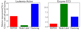
We study the improvement obtained by using self-paced fine-tuning in GShot over vanilla fine-tuning on different metrics. For a metric $P$, we define the improvement as $\frac{P_{\textsc{GShot}(vanilla)}-P_{\textsc{GShot}}}{P_{\textsc{GShot}}}\times 100$. Here, $P_{\textsc{GShot}}$ refers to the value of the metric $P$ obtained by our default model (with self-paced fine tuning), and $P_{\textsc{GShot}(vanilla)}$ refers to the value obtained by GShot with vanilla fine-tuning. In Fig. 5 we observe that a self-paced fine-tuning strategy can improve the fidelity metrics significantly.

Appendix F Impact of auxiliary datasets

In this section, we study the performance of our proposed architecture by selecting different auxiliary datasets during meta-training. Towards this, we choose Enzyme dataset since it consists of $5$ auxiliary datasets and has reasonable scope to sample multiple sets of auxiliary datasets from it. For this experiment we sample(without repetition) sets of $3$ auxiliary datasets $5$ times(eg:- {EC1, EC4, EC5}, {EC2, EC5, EC6} etc.). We train $5$ GShot models with these $5$ different sets of auxiliary datasets. We then fine-tune these $5$ trained models on the target dataset(EC3). We use the same set of auxiliary datasets for training the PreTrain+FT baseline. In Table F, we report the mean performance on each metric along with standard deviation obtained using these $5$ models. For results of training GraphGen and GraphRNN from scratch directly on the target dataset EC3(without auxiliary datasets), refer to Table 4.1 in the main paper.

Table 4: Performance on variation of auxiliary datasets: Performance comparison on the Enzyme EC3 dataset when different sets of auxiliary datasets are used for meta-training GShot and for training the PreTrain+FT baseline. For GShot and PreTrain+FT, we report the mean and standard deviation since their performance is averaged across models using different sets of auxiliary datasets used for (meta/pre) training.

Target dataset

Model

Deg.

Clus.

Orbit

NSPDK

Avg # Nodes (Gen/Gold)

Avg # Edges (Gen/Gold)

Node Label

Edge Label

Joint Node Label & Degree

Novelty

Uniqueness

Enzyme:EC3 #Training samples=50

PreTrain+FT

0.731

0.585

0.060

0.191

20.596/26.90

28.658/52.85

0.006

x

0.644

98.50%

98.70%

$\pm$0.077

$\pm$0.066

$\pm$0.012

$\pm$0.007

$\pm$1.150

$\pm$1.265

$\pm$0.002

x

$\pm$0.026

$\pm$0.005

$\pm$0.004

GShot

0.710

0.554

0.053

0.188

20.742/26.90

29.212/52.85

0.004

x

0.634

98.11%

98.12%

$\pm$0.07

$\pm$0.067

$\pm$0.009

$\pm$ 0.005

$\pm$ 1.04

$\pm$ 1.27

$\pm$ 0.001

x

$\pm$0.018

$\pm$ 0.008

$\pm$ 0.009

In Table F, we observe that GShot obtains superior performance when trained using different sets of auxiliary datasets. For instance, on the Node label metric, GShot outperforms its closest competitor PreTrain+FT by around $50\%$. Further, it outperforms its closest competitor by over $10\%$ on the Orbit metric. Overall, we observe that GShot learns to better utilize the knowledge gained from a variety of auxiliary datasets.

Appendix G Learning to conditionally predict elements of edge tuple of DFS code

We assumed independence between components of edge tuple in order to simplify the modeling process. We also performed experiments by removing the independence assumption and making the prediction of components of edge tuple $\left\langle t_{u},t_{v},L_{u},L_{uv},L_{v}\right\rangle$ conditional on other elements. In order to model the conditional distribution, an order has to be imposed on the components of an edge tuple $\left\langle t_{u},t_{v},L_{u},L_{uv},L_{v}\right\rangle$. As discussed in Sec. 3.2, in the generation process of DFS code for a graph, first a node is discovered and consequently its discovery time $t_{u}$ is recorded. Since this component depends upon the hidden state of the DFS code sequence, we first predict the timestamp $t_{u}$ of the edge tuple using the hidden state $h_{i}$ of LSTM. Now, in order to form an edge, the node with timestamp $t_{u}$ is to be connected to node with discovery timestamp $t_{v}$. Since $t_{v}$ depends upon the hidden state $h_{i}$ and the timestamp $t_{u}$ of the discovered node, we concatenate the hidden state embedding $h_{i}$ and embedding $emb(t_{u})$ of the timestamp $t_{u}$ and predict the timestamp $t_{v}$. Now, for the remaining three components $L_{u}$ , $L_{v}$ and $L_{uv}$, we first predict the label of $u$ and then $v$ in order. This choice promises to improve likelihood of generating node labels $L_{v}$ that have high probability of forming edges with nodes having label $L_{u}$ and vice-versa. Finally, since the edge label between two nodes is a function of the node type(labels), therefore, we condition the edge label $L_{uv}$ on the embedding of labels $L_{u}$ and $L_{v}$ of the edge tuple. The details of the conditional modeling are presented below:

$$t_{u} =MLP(\mathbf{h}_{i})$$

$$t_{v} =MLP(\mathbf{h}_{i}|emb(t_{u}))$$

$$L_{u} =MLP(\mathbf{h}_{i}|emb(t_{u})|emb(t_{v}))$$

$$L_{v} =MLP(\mathbf{h}_{i}|emb(t_{u})|emb(t_{v})|emb(L_{u}))$$

$$L_{uv} =MLP(\mathbf{h}_{i}|emb(t_{u})|emb(t_{v})|emb(L_{u})|emb(L_{v}))$$

Here $emb$ refers to learnable embedding layer whose parameters are learnt during the training process.

Target dataset	Model	Deg.	Clus.	Orbit	NSPDK	Avg # Nodes (Gen/Gold)	Avg # Edges (Gen/Gold)	Node Label	Edge Label	Joint Node Label & Degree	Novelty	Uniqueness
Leukemia-Active	GShot (Ind)	${0.0069}$	$\approx$ 0	$\approx$ 0	0.032	42.35/47.71	44.33/50.37	0.0011	$\approx$ 0	0.24	100%	100%
	GShot (Cond)	${0.01}$	$\approx$ 0.003	$\approx$ 0	0.06	46.37/47.71	49.23/50.37	0.003	$\approx$ 0	0.44	100%	100%
AIDS-CA	GShot (Ind)	0.017	0.0015	$\approx$ 0	0.08	26.5/37.14	27.1/39.60	0.011	$\approx$ 0	0.14	99%	99%
	GShot (Cond)	0.01	0.004	$\approx$ 0	0.07	28.44/37.14	30.50/39.60	0.007	$\approx$ 0	0.12	98.33%	98.43%
Enzyme EC3	GShot (Ind)	0.45	0.47	0.025	0.16	24.5/26.90	37.69/52.85	0.004	x	0.457	100%	100%
	GShot (Cond)	0.43	0.60	0.03	0.20	27.50/26.90	42.55/52.85	0.007	x	0.58	99.4%	98.8%

Table 5: Conditional vs Independent modeling of edge tuple: Performance obtained by different models on different datasets on multiple metrics when components of edge tuples are predicted independently(Ind) vs when they are predicted conditionally(Cond).

To evaluate the performance of the above conditional prediction of the edge tuple, we ran experiments on the target dataset Leukemia-Active, Enzyme EC3 and AIDS-CA dataset . The results are presented in table 5. We denote the model with Independence assumption(default) as Ind, and the model with conditional prediction of components in edge tuple as Cond. On all datasets we observe that for the metrics Avg #nodes and Avg #edges, the models with conditional modeling of edge tuple convincingly outperforms the model(s) with the independence assumption. This signifies that sequence length has been better modelled in GShot when components of the edge tuple are modeled conditionally in comparison to when modeled independently. However, on the other distance metrics, we do not observe clear performance improvements.

Appendix H Using transformer for sequence Modelling

We integrated transformer [35] for modeling the sequences. We present the results in the table  6 when compared with current LSTM-based architecture.

On all datasets, we do not observe clear performance improvements.

Target dataset	Model	Deg.	Clus.	Orbit	NSPDK	Avg # Nodes (Gen/Gold)	Avg # Edges (Gen/Gold)	Node Label	Edge Label	Joint Node Label & Degree	Novelty	Uniqueness
Leukemia- Active	GShot (LSTM)	${0.0069}$	$\approx$ 0	$\approx$ 0	0.032	42.35/47.71	44.33/50.37	0.0011	$\approx$ 0	0.24	100	100
	GShot(Transformer)	$0.0256$	$\approx$ 0.0067	$\approx$ 0.0018	0.1983	50.22/47.71	54.57/50.37	0.011	$\approx$ 0.00104	0.522	100	99.85
AIDS-CA	GShot (LSTM)	0.017	0.0015	$\approx$ 0	0.08	26.5/37.14	27.1/39.60	0.011	$\approx$ 0	0.14	99%	99%
	GShot (Transformer)	0.03044	0.001543	0.000680	0.100	27.10/37.14	28.64/39.60	0.02865	0.00089	0.2220	100%	99.70%
Enzyme EC3	GShot (LSTM)	0.45	0.47	0.025	0.16	24.5/26.90	37.69/52.85	0.004	x	0.457	100%	100%
	GShot (Transformer)	0.7827	0.5871	0.06490	0.2677	25.58/26.90	35.99/ 52.85	0.0177	x	0.6508	96.28%	97.38%

Table 6: Comparison of Transformer based model with LSTM(default) based modeling.

Appendix I Similarity of Target Dataset with Auxiliary Datasets and Impact on Performance

Target dataset	Auxiliary Dataset	Deg.	Clus.	Orbit	NSPDK	Avg # Nodes (Target/Aux)	Avg # Edges (Target/Aux)	Node Label	Edge Label	Joint Node Label & Degree
Leukemia-Active	Breast	0.007	0.0008	0.0003	0.07	47.0/55.83	49.61/59.35	0.007	$\approx$ 0	0.029
	Lung	0.001	$\approx$ 0	0.0002	0.065	47.0/40.0	49.61/41.82	0.012	$\approx$ 0	0.05
	Yeast	0.0044	$\approx$ 0	$\approx$ 0	0.07	47.0/32.70	49.61/34.03	0.02	0.002	0.059
	Enzyme EC1	1.41	1.28	0.16	0.47	47.0/29.73	49.61/58.52	1.85	x	1.15
	Enzyme EC2	1.33	1.22	0.15	0.49	47.0/32.88	49.61/63.16	1.91	x	1.36
	Enzyme EC3	1.36	1.28	0.25	0.47	47.0/28.91	49.61/56.50	1.87	x	1.16
	Enzyme EC4	1.39	1.18	0.22	0.48	47.0/37.47	49.61/74.00	1.90	x	1.25
	Enzyme EC5	1.23	1.12	0.10	0.46	47.0/27.61	49.61/51.17	1.89	x	1.09
	Enzyme EC6	1.28	1.31	0.09	0.48	47.0/30.49	49.61/60.01	1.90	x	1.34
Enzyme EC3	Enzyme EC1	0.042	0.20	0.03	0.055	28.35/39.85	53.89/70.63	0.007	x	0.08
	Enzyme EC2	0.024	0.09	0.04	0.055	28.35/28.44	53.89/70.63	0.029	x	0.12
	Enzyme EC4	0.021	0.11	0.008	0.050	28.35/37.79	53.89/74.27	0.012	x	0.047
	Enzyme EC5	0.007	0.088	0.008	0.056	28.35/33.6	53.89/64.33	0.024	x	0.05
	Enzyme EC6	0.031	0.42	0.05	0.054	28.35/30.33	53.89/59.99	0.019	x	0.096
	Yeast	1.39	1.28	0.27	0.47	28.35/34.63	53.89/56.09	1.86	x	1.11
	Breast	1.37	1.287	0.26	0.49	28.35/44.01	53.89/46.26	1.89	x	1.15
	Lung	1.39	1.288	0.271	0.46	28.35/36.63	53.89/38.40	1.875	x	1.121

Table 7: Distance of target datasets with different auxiliary datasets on a variety of distance metrics. The auxiliary datasets highlighted in bold are highly similar to the target datasets.

We compare our target datasets specifically Enzyme EC3 and Leukemia-Active with a variety of auxiliary datasets on different graph distance metrics in Table 7 below. For instance, we observe that Leukemia-Active target dataset has more similarities with chemical datasets such as Breast, Lung and Yeast. Additionally, we observe it is highly dis-similar with datasets belonging to Enzyme(Biological) category. Similarly, in Table  7 below we observe that Enzyme EC3 dataset is highly similar to other Enzyme datasets and dis-similar to datasets such as Breast, Lung and Yeast.

Further, to understand the impact of choosing different auxiliary datasets based upon their similarity to target dataset, we train GShot with different sets of auxiliary datasets. In Table  8, we observe GShot convincingly performs better when auxiliary datasets that are similar to target datasets are chosen for meta-training. Specifically, GShot trained with Yeast,Breast and Lung as auxiliary datasets significantly outperforms GShot meta-trained with Enzyme datasets, when the target dataset is Leukemia-Active. Similar conclusion is observed on Enzyme EC3 dataset in Table  8.

Target dataset	Auxiliary Dataset	Model	Deg.	Clus.	Orbit	NSPDK	Avg # Nodes (Gen/Gold)	Avg # Edges (Gen/Gold)	Node Label	Edge Label	Joint Node Label & Degree	Novelty	Uniqueness
Leukemia-Active	Yeast, Breast, Lung	GShot	${0.0069}$	$\approx$ 0	$\approx$ 0	0.032	42.35/47.71	44.33/50.37	0.0011	$\approx$ 0	0.24	100%	100%
	Enzyme(1,2,3,4,5,6)	GShot	0.07	0.005	0.001	0.20	39.38/47.71	41.32/50.37	0.022	$\approx$ 0	1.08	100%	100%
Enzyme EC3	Enzyme(1,2,4,5,6)	GShot	0.45	0.47	0.025	0.16	24.5/26.90	37.69/52.85	0.004	x	0.457	100%	100%
	Yeast, Lung, Breast	GShot	0.54	0.62	0.029	0.21	22.89/26.90	34.33/52.85	0.007	$\approx 0$	0.62	99.8%	99.8%

Table 8: Impact of different auxiliary datasets on quality of GShot. We observe that when auxiliary datasets are similar to target dataset(as per table 7), the performance of GShot is significantly better.

References

- You et al. [2018a] Jiaxuan You, Bowen Liu, Rex Ying, Vijay Pande, and Jure Leskovec. Graph convolutional policy network for goal-directed molecular graph generation. In NeurIPS, NIPS’18, page 6412–6422, Red Hook, NY, USA, 2018a. Curran Associates Inc.
- Goyal et al. [2020] Nikhil Goyal, Harsh Vardhan Jain, and Sayan Ranu. Graphgen: a scalable approach to domain-agnostic labeled graph generation. In Proceedings of The Web Conference 2020, pages 1253–1263, 2020.
- De Cao and Kipf [2018] Nicola De Cao and Thomas Kipf. MolGAN: An implicit generative model for small molecular graphs. ICML 2018 workshop on Theoretical Foundations and Applications of Deep Generative Models, 2018.
- Bojchevski et al. [2018] Aleksandar Bojchevski, Oleksandr Shchur, Daniel Zügner, and Stephan Günnemann. Netgan: Generating graphs via random walks. In Proceedings of the 35th International Conference on Machine Learning, ICML 2018, Stockholmsmässan, Stockholm, Sweden, July 10-15, 2018, pages 609–618, 2018.
- Albert and Barabási [2002] Réka Albert and Albert-László Barabási. Statistical mechanics of complex networks. Reviews of modern physics, 74(1):47, 2002.
- Liao et al. [2019] Renjie Liao, Yujia Li, Yang Song, Shenlong Wang, Charlie Nash, William L. Hamilton, David Duvenaud, Raquel Urtasun, and Richard Zemel. Efficient graph generation with graph recurrent attention networks. In NeurIPS, 2019.
- Simonovsky and Komodakis [2018] Martin Simonovsky and Nikos Komodakis. Graphvae: Towards generation of small graphs using variational autoencoders. In Vera Kurková, Yannis Manolopoulos, Barbara Hammer, Lazaros S. Iliadis, and Ilias Maglogiannis, editors, Artificial Neural Networks and Machine Learning - ICANN 2018, volume 11139 of Lecture Notes in Computer Science, pages 412–422, 2018.
- Gupta et al. [2022] Shubham Gupta, Sahil Manchanda, Srikanta Bedathur, and Sayan Ranu. Tigger: Scalable generative modelling for temporal interaction graphs. In Proceedings of the AAAI Conference on Artificial Intelligence, volume 36, pages 6819–6828, 2022.
- Gupta and Bedathur [2022] Shubham Gupta and Srikanta Bedathur. A survey on temporal graph representation learning and generative modeling, 2022.
- Jain et al. [2021] Jayant Jain, Vrittika Bagadia, Sahil Manchanda, and Sayan Ranu. Neuromlr: Robust & reliable route recommendation on road networks. Advances in Neural Information Processing Systems, 34:22070–22082, 2021.
- Borgwardt et al. [2005] Karsten M. Borgwardt, Cheng Soon Ong, Stefan Schönauer, S. V. N. Vishwanathan, Alexander J. Smola, and Hans-Peter Kriegel. Protein function prediction via graph kernels. Bioinformatics, 21 Suppl 1:i47–56, 2005.
- [12] U.S. National Library of Medicine National Center for Biotechnology Information. Pubchem. URL http://pubchem.ncbi.nlm.nih.gov.
- You et al. [2018b] Jiaxuan You, Rex Ying, Xiang Ren, William L. Hamilton, and Jure Leskovec. Graphrnn: Generating realistic graphs with deep auto-regressive models. In ICML, 2018, volume 80 of Proceedings of Machine Learning Research, pages 5694–5703. PMLR, 2018b.
- Bartunov and Vetrov [2018] Sergey Bartunov and Dmitry Vetrov. Few-shot generative modelling with generative matching networks. In International Conference on Artificial Intelligence and Statistics, pages 670–678. PMLR, 2018.
- Swinney and Xia [2014] David C Swinney and Shuangluo Xia. The discovery of medicines for rare diseases. Future medicinal chemistry, 6(9):987–1002, 2014.
- Cui et al. [2020] Wen Cui, Kailin Yang, and Haitao Yang. Recent progress in the drug development targeting sars-cov-2 main protease as treatment for covid-19. Frontiers in Molecular Biosciences, 7, 2020. ISSN 2296-889X.
- Kipf et al. [2018] Thomas Kipf, Ethan Fetaya, Kuan-Chieh Wang, Max Welling, and Richard Zemel. Neural relational inference for interacting systems. In International Conference on Machine Learning, pages 2688–2697, 2018.
- Perraudin et al. [2019] Nathanaël Perraudin, Ankit Srivastava, Aurelien Lucchi, Tomasz Kacprzak, Thomas Hofmann, and Alexandre Réfrégier. Cosmological n-body simulations: a challenge for scalable generative models. Computational Astrophysics and Cosmology, 6(1):1–17, 2019.
- Yuanqi [2021] Yuanqi. Graphgt: Machine learning datasets for graph generation and transformation. In Thirty-fifth Conference on Neural Information Processing Systems Datasets and Benchmarks Track (Round 2), 2021.
- Irwin and Shoichet [2005] John J Irwin and Brian K Shoichet. Zinc- a free database of commercially available compounds for virtual screening. Journal of chemical information and modeling, 45(1):177–182, 2005.
- Finn et al. [2017] Chelsea Finn, Pieter Abbeel, and Sergey Levine. Model-agnostic meta-learning for fast adaptation of deep networks. In International conference on machine learning, pages 1126–1135. PMLR, 2017.
- Manchanda et al. [2022] Sahil Manchanda, Sofia Michel, Darko Drakulic, and Jean-Marc Andreoli. On the generalization of neural combinatorial optimization heuristics. In Joint European Conference on Machine Learning and Knowledge Discovery in Databases, pages 426–442. Springer, 2022.
- Yan [2002] Xifeng Yan. gspan: Graph-based substructure pattern mining. In Proceedings of the 2002 IEEE International Conference on Data Mining (ICDM 2002), 9-12 December 2002, Maebashi City, Japan, pages 721–724, 2002.
- Hochreiter and Schmidhuber [1997] Sepp Hochreiter and Jürgen Schmidhuber. Long Short-Term Memory. Neural Computation, 9(8):1735–1780, 11 1997. ISSN 0899-7667.
- Nichol and Schulman [2018] Alex Nichol and John Schulman. Reptile: a scalable metalearning algorithm. arXiv preprint arXiv:1803.02999, 2(3):4, 2018.
- Zaremba and Sutskever [2015] Wojciech Zaremba and Ilya Sutskever. Learning to execute, 2015.
- Kumar et al. [2010] M. Kumar, Benjamin Packer, and Daphne Koller. Self-paced learning for latent variable models. In NeurIPS, volume 23. Curran Associates, Inc., 2010.
- Kawai et al. [2019] Wataru Kawai, Yusuke Mukuta, and Tatsuya Harada. GRAM: scalable generative models for graphs with graph attention mechanism. CoRR, abs/1906.01861, 2019.
- Hočevar and Demšar [2014] Tomaž Hočevar and Janez Demšar. A combinatorial approach to graphlet counting. Bioinformatics, 30(4):559–565, 2014.
- Gretton et al. [2012] Arthur Gretton, Karsten M. Borgwardt, Malte J. Rasch, Bernhard Schölkopf, and Alexander J. Smola. A kernel two-sample test. J. Mach. Learn. Res., 13:723–773, 2012.
- Costa [2010] Fabrizio Costa. Fast neighborhood subgraph pairwise distance kernel. In ICML, pages 255–262, 2010.
- Ingraham et al. [2019] John Ingraham, Vikas Garg, Regina Barzilay, and Tommi Jaakkola. Generative models for graph-based protein design. Advances in Neural Information Processing Systems, 32, 2019.
- Guo et al. [2020] Xiaojie Guo, Yuanqi Du, Sivani Tadepalli, Liang Zhao, and Amarda Shehu. Generating tertiary protein structures via an interpretative variational autoencoder. arXiv preprint arXiv:2004.07119, 2020.
- Schomburg et al. [2004] Ida Schomburg, Antje Chang, Christian Ebeling, Marion Gremse, Christian Heldt, Gregor Huhn, and Dietmar Schomburg. Brenda, the enzyme database: updates and major new developments. Nucleic acids research, 32 Database issue:D431–3, 2004.
- Vaswani et al. [2017] Ashish Vaswani, Noam Shazeer, Niki Parmar, Jakob Uszkoreit, Llion Jones, Aidan N Gomez, Ł ukasz Kaiser, and Illia Polosukhin. Attention is all you need. In I. Guyon, U. Von Luxburg, S. Bengio, H. Wallach, R. Fergus, S. Vishwanathan, and R. Garnett, editors, Advances in Neural Information Processing Systems, volume 30. Curran Associates, Inc., 2017. URL https://proceedings.neurips.cc/paper_files/paper/2017/file/3f5ee243547dee91fbd053c1c4a845aa-Paper.pdf.