Dispersive determination of neutrino mass ordering

Abstract

We argue that the mixing phenomenon of a neutral meson formed by a fictitious massive quark will disappear, if the electroweak symmetry of the Standard Model (SM) is restored at a high energy scale. This disappearance is taken as the high-energy input for the dispersion relation, which must be obeyed by the width difference between two meson mass eigenstates. The solution to the dispersion relation at low energy, i.e., in the symmetry broken phase, then connects the Cabibbo-Kobayashi-Maskawa (CKM) matrix elements to the quark masses involved in the box diagrams responsible for meson mixing. It is demonstrated via the analysis of the $D$ meson mixing that the typical $d$, $s$ and $b$ quark masses demand the CKM matrix elements in agreement with measured values. In particular, the known numerical relation $V_{us}\approx\sqrt{m_{s}/m_{b}}$ with the $s$ ($b$) quark mass $m_{s}$ ($m_{b}$) can be derived analytically from our solution. Next we apply the same formalism to the mixing of the $\mu^{-}e^{+}$ and $\mu^{+}e^{-}$ states through similar box diagrams with intermediate neutrino channels. It is shown that the neutrino masses in the normal hierarchy (NH), instead of in the inverted hierarchy or quasi-degenerate spectrum, match the observed Pontecorvo-Maki-Nakagawa-Sakata matrix elements. The lepton mixing angles larger than the quark ones are explained by means of the inequality $m_{2}^{2}/m_{3}^{2}\gg m_{s}^{2}/m_{b}^{2}$, $m_{2,3}$ being the neutrino masses in the NH. At last, the solution for the $\tau^{-}e^{+}$-$\tau^{+}e^{-}$ mixing specifies the mixing angle $\theta_{23}\approx 45^{\circ}$. Our work suggests that the fermion masses and mixing parameters are constrained dynamically, and the neutrino mass orderings can be discriminated by the internal consistency of the SM.

I INTRODUCTION

It has been believed that the parameters in the Standard Model (SM), such as particle masses and mixing angles, are free, and have to be determined experimentally. These parameters originate from the independent elements of the Yukawa matrices, which cannot be completely constrained by symmetries Santamaria:1993ah , as the electroweak symmetry is broken. Any attempt to explain their values relies on an underlying new physics theory existent at high energy, whose low-energy behavior fixes the SM parameters. However, the above observation is made at the Lagrangian level without taking into account subtle dynamical interplay among the involved gauge and scalar sectors. We have pointed out in recent publications Li:2023dqi ; Li:2023yay that dispersion relations, which physical observables must obey owing to analyticity, connect various interactions at different scales, and thus impose stringent constraints on the SM parameters. The SM parameters should satisfy dispersive constraints from all physical observables in principle. We have demonstrated, by considering those which provide efficient constraints Li:2023dqi ; Li:2023yay , that at least some of the SM parameters can be determined dynamically within the model itself.

A dispersion relation links the high- and low-energy properties of an observable, which is defined by a correlation function. The high-energy property, calculated perturbatively from the correlation function, is treated as an input. The low-energy property is then solved directly from the dispersion relation with the given input, which demands specific values for relevant particle masses in agreement with measured ones. We have analyzed heavy meson decay widths Li:2023dqi , written as absorptive pieces of hadronic matrix elements of four-quark effective operators, in this inverse-problem approach Li:2020xrz ; Li:2020fiz ; Li:2020ejs ; Xiong:2022uwj . Starting with massless final-state $u$ and $d$ quarks, we found that the solution for the decay $c\to du\bar{d}$ ($b\to c\bar{u}d$) with heavy-quark-expansion (HQE) inputs leads to the $c$ ($b$) quark mass $m_{c}=1.35$ ($m_{b}=4.0$) GeV. The requirement that the dispersion relation for the $c\to su\bar{d}$ ($c\to d\mu^{+}\nu_{\mu}$, $b\to u\tau^{-}\bar{\nu}_{\tau}$) decay yields the same heavy quark mass fixes the strange quark (muon, $\tau$ lepton) mass $m_{s}=0.12$ GeV ($m_{\mu}=0.11$ GeV, $m_{\tau}=2.0$ GeV). The investigation on the dispersion relation respected by the correlation function of two $b$-quark scalar (vector) currents, with the input from the perturbative evaluation of the $b$ quark loop, returns the Higgs ($Z$) boson mass 114 (90.8) GeV Li:2023yay .

The successful explanation of the particle masses from 0.1 GeV up to the electroweak scale by means of the internal consistency of SM dynamics encourages us to address the fermion mixing in the same formalism. We first argue that the mixing phenomenon of a neutral meson formed by a fictitious massive quark will disappear, if the electroweak symmetry of the SM is restored at a high energy scale Chien:2018ohd ; Huang:2020iya . This disappearance is taken as the high-energy input for the dispersion relation satisfied by the width difference between two meson mass eigenstates. The solution to the dispersion relation at low energy, i.e., in the symmetry broken phase, effectively binds the Cabibbo-Kobayashi-Maskawa (CKM) matrix elements and the quark masses appearing in the box diagrams responsible for meson mixing. It will be elaborated how the typical $d$, $s$ and $b$ quark masses constrain the Cabibbo-Kobayashi-Maskawa (CKM) matrix elements through the dispersive analysis of the $D$ meson mixing. The connection between the fermion flavor structure and the pattern of the Yukawa matrices, together with plausible relations among the quark masses and the mixing angles, have been speculated HF78 ; CS87 . For a recent reference in this direction based on Yukawa matrix textures, see Belfatto:2023qca . We will derive the known numerical relation $V_{us}\approx\sqrt{m_{s}/m_{b}}$ Belfatto:2023qca with the $s$ ($b$) quark mass $m_{s}$ ($m_{b}$) analytically from our solution. Namely, our work realizes the speculation in the literature, and suggests that its underlying theory is the SM itself.

We then perform the similar analysis of the mixing between the $\mu^{-}e^{+}$ and $\mu^{+}e^{-}$ states, which occurs via the box diagrams involving intermediate neutrino channels. The formulas are exactly the same as of the $D$ meson, i.e., $c\bar{u}$-$\bar{c}u$ mixing, with the quark masses $m_{d,s,b}$ being replaced by the neutrino masses $m_{1,2,3}$, and the CKM matrix elements by the Pontecorvo–Maki–Nakagawa–Sakata (PMNS) ones. It will be shown that the neutrino masses in the normal hierarchy (NH), instead of in the inverted hierarchy (IH) or quasi-degenerate (QD) spectrum, match the observed PMNS matrix elements. The neutrino mass ordering, whose various scenarios have not been discriminated experimentally, has remained as an unsettled issue in neutrino physics PDG . Our study provides a solid theoretical support for the NH spectrum in the viewpoint of the internal consistency of SM dynamics. The neutrino mixing angles larger than the quark ones are then accounted for naturally by the inequality $m_{2}^{2}/m_{3}^{2}\gg m_{s}^{2}/m_{b}^{2}$ for $m_{2,3}$ in the NH. We further examine the $\tau^{-}e^{+}$-$\tau^{+}e^{-}$ mixing, and find that its solution requests the angle $\theta_{23}\approx 45^{\circ}$ in accordance with its observed value around the maximal mixing. It is emphasized that the above relations between the fermion masses and mixing angles are established without resorting to specific new ingredients beyond the SM (for recent endeavors on this topic, refer to Alvarado:2020lcz ; Xu:2023kfi ; Patel:2023qtw ; Bora:2023teg ; Thapa:2023fxu ).

II FORMALISM

There are models in the literature, which provide a suitable framework for our discussion based on the restoration of the electroweak symmetry. For example, the composite Higgs model proposed in Kaplan:1983fs meets the purpose well. The electroweak group in their model is broken at a scale much lower than the condensate scale, implying the existence of a symmetry restoration scale which we refer to. It has been known that this feature is crucial for explaining the light SM Higgs boson mass in the composite Higgs model. The disappearance of the mixing phenomenon mentioned in the Introduction takes place in the region above the restoration scale and below the condensate scale. We do not intend to elaborate the detail of this model here, but to establish the dispersive constraints that some SM parameters should satisfy, if the electroweak symmetry is restored. It is likely that the interesting observations made in present work may give a hint on model building at high energy, as remarked in the conclusion section.

Consider the mixing mechanism of a neutral meson formed by a fictitious massive quark $Q$ before and after the electroweak symmetry breaking in the SM. Precisely, we work on the mixing between the $Q_{L}\bar{q}_{L}$ and $\bar{Q}_{L}q_{L}$ states, where $q$ is a light quark and the subscript $L$ denotes the left handedness. Before the symmetry breaking, all particles are massless, and quarks are in their flavor eigenstates. The meson mixing happens through exchanges of charged or neutral scalars among quarks, whose strengths are characterize by the Yukawa couplings. After the symmetry breaking, particles get masses and quarks are turned into the mass eigenstates by the unitary field transformations. The neutral scalar currents, coupling left- and right-handed quarks, become diagonal in flavor space under the above transformations. The neutral vector currents, which couple quarks of the same handedness and are diagonal in flavor space before the symmetry breaking, continue to be diagonal. This is the reason why the flavor-changing neutral currents, either scalar or vector, are absent in the SM. The neutral meson mixing in the symmetry broken phase then takes places via $W$ boson exchanges between quarks, whose strengths are proportional to the CKM matrix elements.

The Yukawa matrices have the same number of independent parameters as the CKM matrix and the quark masses have, i.e., nine moduli and one phase Santamaria:1993ah . It is hard to trace these independent parameters, if one discusses neutral meson mixing in the symmetric phase based on the Yukawa matrices. A more transparent picture is attained by implementing the quark field transformations adopted in the symmetry broken phase. The Yukawa matrices are then diagonalized, but the charged scalar currents persist. Besides, the up-type (down-type) quarks, which couple to the down-type (up-type) quarks in the mass eigenstates through the charged scalar currents, are not in the mass eigenstates. Neutral meson mixing is induced only by the charged currents after the above quark field transformations. The exchanges of one charged scalar and one $W$ boson are excluded, for they cause the mixing between the $Q_{L}\bar{q}_{L}$ and $\bar{Q}_{R}q_{R}$ states. The contributions from $W$ boson exchanges are associated with the CKM factors, which respect the unitarity. Since all intermediate quarks are massless in the symmetric phase, these contributions cancel among contained channels. As to the charged scalar exchanges, the intermediate quarks are not in the mass eigenstates, but still orthogonal to each other. Hence, the diagonal Yuakawa matrices forbid the charged scalars to contribute to neutral meson mixing. We conclude that the mixing phenomenon disappears as the electroweak symmetry is restored at a high energy scale. The vanishing of a mixing observable at high energy will be treated as an input in the dispersive analysis below.

The dispersion relation for neutral meson mixing is quoted as Li:2022jxc

$$M_{12}(s)=\frac{1}{2\pi}\int ds^{\prime}\frac{\Gamma_{12}(s^{\prime})}{s-s^{\prime}},$$ (1)

where $s$ is the mass squared of the quark $Q$ Li:2020xrz , and the application of the principal-value prescription to the right-hand side is implicit. The proposed contour and the location of $s$ have been described in Fig. 1 of Ref. Li:2022jxc . In the above expression $M_{12}(s)$ and $\Gamma_{12}(s)$ represent the real and imaginary pieces of the box-diagram contribution, respectively, which governs the time evolution of the fictitious neutral meson. Their analytical properties can be inferred from the explicit expressions in Appendix A of Ref. BSS . Simply speaking, the box-diagram contribution has no poles but contains branch cuts along the real axis with the thresholds being specified below. The piece $\Gamma_{12}$ is related to the width difference between the two meson mass eigenstates. As $s$, i.e., the scale involved in the box diagrams is large enough, the electroweak symmetry is restored and all intermediate particles become massless. The argument holding for the symmetric phase then implies $M_{12}(s)\approx 0$ at large $s$ owing to the disappearance of the mixing phenomenon. We mention an alternative setup for the same purpose, $Q_{L}\bar{q}_{L}$ scattering into $\bar{Q}_{L}q_{L}$ at arbitrary center-of-mass energy $E$. As $E$ is high enough, all intermediate particles become massless, and the corresponding amplitude diminishes.

The dispersive integral on the right-hand side of Eq. (1) receives the low-mass contribution from $\Gamma_{12}$, which depends on the CKM matrix elements associated with various massive intermediate quarks in the symmetry broken phase. It has been illustrated that the physical $\Gamma_{12}$ with hadronic thresholds and the perturbative $\Gamma_{12}$ from the box diagrams with quark-level thresholds produce the same dispersive integral Li:2022jxc . This equality has allowed us to solve for the physical $\Gamma_{12}$ from the dispersion relation, which accommodates the observed large $D$ meson mixing parameters. Here we adopt the perturbative $\Gamma_{12}$ as evaluating the dispersive integral in Eq. (1) for simplicity. The box diagrams generate the $(V-A)(V-A)$ and $(S-P)(S-P)$ effective operators, which should be handled independently. We concentrate on the former contribution, which is expressed as BSS ; Cheng

$$\Gamma_{12}(s) \propto \sum_{i,j}\lambda_{i}\lambda_{j}\Gamma_{ij}(s),$$

$$\Gamma_{ij}(s) = \frac{1}{s^{2}}\frac{\sqrt{s^{2}-2s(m_{i}^{2}+m_{j}^{2})+(m_{i}^{2}-m_{j}^{2})^{2}}}{(m_{W}^{2}-m_{i}^{2})(m_{W}^{2}-m_{j}^{2})}$$ (2)

$$\times\left\{\left(m_{W}^{4}+\frac{m_{i}^{2}m_{j}^{2}}{4}\right)[2s^{2}-4s(m_{i}^{2}+m_{j}^{2})+2(m_{i}^{2}-m_{j}^{2})^{2}]+3m_{W}^{2}s(m_{i}^{2}+m_{j}^{2})(m_{i}^{2}+m_{j}^{2}-s)\right\},$$

with the $W$ boson mass $m_{W}$ and the intermediate quark masses $m_{i}$ and $m_{j}$. The overall coefficient, including the bag parameter and the meson decay constant which are irrelevant to the reasoning below, has been suppressed. For the $D$ meson mixing, $i,j=d,s,b$ label the down-type quarks, and $\lambda_{i}\equiv V^{*}_{ci}V_{ui}$ are the products of the CKM matrix elements. It will be verified that the same conclusion is drawn, when the analysis is performed based on the perturbative contribution from the $(S-P)(S-P)$ operator.

It seems that the $W$ bosons in the box diagrams for the $c\bar{u}$-$\bar{c}u$ mixing can be integrated out. First, Eq. (2) has appeared in the dispersive determination of the top quark mass from the $t\bar{u}$-$\bar{t}u$ mixing Li:2023yay , and the implication on the present subject from this mixing will be discussed in Sec. IV. The $W$ boson fields should not be integrated out in this case. More importantly, the box-diagram contribution in the asymptotic region with high $s$ is crucial for deriving the constraints on fermion masses and mixing angles as seen shortly, in which heavy gauge bosons should remain dynamical. It is thus appropriate to quote the formulas in BSS ; Cheng directly with the $m_{W}$ dependence being kept. Note that in our previous study on heavy meson decay widths Li:2023dqi , we focused on the explanation of the heavy quark masses below the $W$ boson mass $m_{W}$, which prefers the employment of the effective theory with $W$ boson fields being integrated out.

To diminish the dispersive integral in Eq. (1) for arbitrary large $s$, some conditions must be met by the CKM matrix elements. Notice the asymptotic behavior of Eq. (2)

$$\Gamma_{ij}(s^{\prime})\approx\Gamma^{(1)}_{ij}s^{\prime}+\Gamma^{(0)}_{ij}+\frac{\Gamma^{(-1)}_{ij}}{s^{\prime}}+\cdots,$$ (3)

with the coefficients

$$\Gamma^{(1)}_{ij} = \frac{4m_{W}^{4}-6m_{W}^{2}(m_{i}^{2}+m_{j}^{2})+m_{i}^{2}m_{j}^{2}}{2(m_{W}^{2}-m_{i}^{2})(m_{W}^{2}-m_{j}^{2})},$$

$$\Gamma^{(0)}_{ij} = -\frac{3(m_{i}^{2}+m_{j}^{2})\left[4m_{W}^{4}-4m_{W}^{2}(m_{i}^{2}+m_{j}^{2})+m_{i}^{2}m_{j}^{2}\right]}{2(m_{W}^{2}-m_{i}^{2})(m_{W}^{2}-m_{j}^{2})},$$

$$\Gamma^{(-1)}_{ij} = \frac{3(m_{i}^{4}+m_{j}^{4})\left[4m_{W}^{4}-2m_{W}^{2}(m_{i}^{2}+m_{j}^{2})+m_{i}^{2}m_{j}^{2}\right]}{2(m_{W}^{2}-m_{i}^{2})(m_{W}^{2}-m_{j}^{2})}.$$ (4)

Each term $\Gamma_{ij}^{(m)}$ gives contributions scaling like $\Lambda^{2}/s$, $(m_{i}^{2}+m_{j}^{2})\Lambda/s$, and $(m_{i}^{4}+m_{j}^{4})\ln\Lambda/s$ for $m=1,0$, and $-1$, respectively, to the dispersive integral in Eq. (1), where $\Lambda$ is of order of the electroweak symmetry restoration scale. Suppression on these contributions characterized by large variable $\Lambda$ is necessary for making finite the dispersive integral, which can be achieved by imposing

$$\sum_{i,j}\lambda_{i}\lambda_{j}\Gamma_{ij}^{(m)}\approx 0,\;\;\;\;m=1,0,-1.$$ (5)

Because the scale $\Lambda$ is not infinite, the left-hand sides of the above relations need not vanish exactly, but to be tiny enough.

Once the conditions in Eq. (5) are fulfilled, we recast the dispersive integral into

$$\int ds^{\prime}\frac{\Gamma_{12}(s^{\prime})}{s-s^{\prime}}\approx\frac{1}{s}\sum_{i,j}\lambda_{i}\lambda_{j}g_{ij},$$ (6)

with the factors

$$g_{ij}\equiv\int_{t_{ij}}^{\infty}ds^{\prime}\left[\Gamma_{ij}(s^{\prime})-\Gamma_{ij}^{(1)}s^{\prime}-\Gamma^{(0)}_{ij}-\frac{\Gamma^{(-1)}_{ij}}{s^{\prime}}\right],$$ (7)

and the thresholds $t_{ij}=(m_{i}+m_{j})^{2}$. The approximation $1/(s-s^{\prime})\approx 1/s$ has been implemented, which holds well for large $s$, since the integral receives contributions only from finite $s^{\prime}$. The integrand in the square brackets decreases like $1/s^{\prime 2}$, so the upper bound of $s^{\prime}$ in Eq. (7) can be extended to infinity safely. We place the final condition

$$\sum_{i,j}\lambda_{i}\lambda_{j}g_{ij}\approx 0,$$ (8)

to ensure the almost nil dispersive integral. That is, the realization of Eqs. (5) and (8) establishes a solution to the dispersion relation in Eq. (1) at large $s$ with $M_{12}(s)\approx 0$.

Some remarks are in order. One may wonder whether the divergent pieces in the dispersive integral in Eq. (1) can be removed by subtraction. As the subtraction is implemented by introducing one power of $s^{\prime}-s_{1}$ into the denominator of the dispersive integral, a subtraction constant $M_{12}(s_{1})$ appears,

$$\frac{M_{12}(s)-M_{12}(s_{1})}{s_{1}-s}=\frac{1}{2\pi}\int ds^{\prime}\frac{\Gamma_{12}(s^{\prime})}{(s-s^{\prime})(s_{1}-s^{\prime})}.$$ (9)

If $s_{1}$ is above the electroweak symmetry restoration scale $\Lambda$, like $s$, we will have $M_{12}(s)\approx 0$, $M_{12}(s_{1})\approx 0$ and $(s-s^{\prime})(s_{1}-s^{\prime})\approx ss_{1}$. The above expression then reduces to $\int ds^{\prime}\Gamma_{12}(s^{\prime})\approx 0$, which produces the conditions identical to Eqs. (5) and (8). If $s_{1}$ is below $\Lambda$, we will have $M_{12}(s)\approx 0$, $s_{1}-s\approx-s$ and $s-s^{\prime}\approx s$. Equation (9) thus turns into the same form as Eq. (1) that we started with. It is more difficult to extract constraints from the dispersion relation with $s_{1}<\Lambda$, and solving such an integral equation is not our strategy. Namely, implementing the subtraction either leaves our formalism unchanged or complicates the analysis, and does not really tame the divergent behavior of the dispersive integral. Note that we stick to the leading-order accuracy in this work as the first attempt to extract the relations among fermion masses and mixing angles by means of analyticity. Higher-order QCD and electroweak corrections, such as those from the channels involving quark pairs through $W$ boson decays, can be taken into account systematically in the future.

III QUARK MASSES AND THE CKM MATRIX

It is apparent that Eqs. (5) and (8) enforce the connections between the CKM matrix elements and the quark masses speculated in the literature, which will be confronted by the measured values below. With the unitarity of the CKM matrix, we rewrite these conditions for the $D$ meson, i.e., $c\bar{u}$-$\bar{c}u$ mixing as

$$r^{2}R_{dd}^{(m)}+2rR_{ds}^{(m)}+1\approx 0,,\;\;\;\;m=1,0,-1,i$$ (10)

with the ratios

$$R_{dd}^{(m)}=\frac{\Gamma_{dd}^{(m)}-2\Gamma_{db}^{(m)}+\Gamma_{bb}^{(m)}}{\Gamma_{ss}^{(m)}-2\Gamma_{sb}^{(m)}+\Gamma_{bb}^{(m)}},\;\;\;\;R_{ds}^{(m)}=\frac{\Gamma_{ds}^{(m)}-\Gamma_{db}^{(m)}-\Gamma_{sb}^{(m)}+\Gamma_{bb}^{(m)}}{\Gamma_{ss}^{(m)}-2\Gamma_{sb}^{(m)}+\Gamma_{bb}^{(m)}},$$ (11)

for $m=1,0,-1$. The expression for $m=i$ is similar with $g_{ij}$ being substituted for $\Gamma_{ij}^{(m)}$ in Eq. (11). We will encounter real $W$-boson production as the massive quark mass exceeds the thresholds $m_{W}+m_{i}$, $m_{W}+m_{j}$ and $2m_{W}$, whose effects are not taken into account in Eq. (2). However, these thresholds, much greater than the other scales in the box diagrams like $m_{b}$, are not expected to make an impact. For example, the region of $s^{\prime}>m_{W}^{2}$ in Eq. (7) contributes only about $10^{-4}$ of the coefficients $R_{dd}^{(i)}$ and $R_{ds}^{(i)}$.

The factor $r$ is defined as the ratio of the CKM matrix elements,

$$r=\frac{\lambda_{d}}{\lambda_{s}}=\frac{V^{*}_{cd}V_{ud}}{V^{*}_{cs}V_{us}}\equiv u+iv,$$ (12)

where the real part $u\equiv{\rm Re}(r)$ and the imaginary part $v\equiv{\rm Im}(r)$ have been introduced. Equation (10) contains both the real and imaginary pieces, which can be treated separately. The imaginary pieces, simply proportional to $v^{2}$, do not provide nontrivial constraints. Therefore, we consider the real pieces, searching for the values of $u$ and $v$ that minimize the squares of these real pieces simultaneously, and then check whether the obtained $u$ and $v$ also diminish the imaginary pieces of the conditions. It is equivalent to eliminate the product $V^{*}_{cd}V_{ud}$ using unitarity and to work on the ratio $V^{*}_{cb}V_{ub}/(V^{*}_{cs}V_{us})$. We have corroborated that this option leads to the same conclusion within theoretical uncertainties.

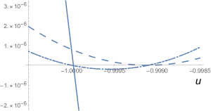
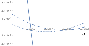
(a)                                                                       (b)

Figure 1: (a) Dependences of $(u^{2}-v^{2})R_{dd}^{(m)}+2uR_{ds}^{(m)}+1$ on $u$ with $v=0$ for $m=1$ (dashed line), $m=0$ (dotted line), $m=-1$ (dash-dotted line), and $m=i$ (solid line). (b) Dependences of $(u^{2}-v^{2})R_{dd}^{(m)}+2uR_{ds}^{(m)}+1$ on $u$ with $v=0.00062$ for $m=1$ (dashed line)), $m=-1$ (dash-dotted line), and $m=i$ (solid line).

To explain how the aforementioned minima is reached, we exhibit the dependencies of the real pieces $(u^{2}-v^{2})^{2}R_{dd}^{(m)}+2uR_{ds}^{(m)}+1$ on $u$ for $v=0$ in Fig. 1(a) with the inputs of the typical quark masses $m_{d}=0.005$ GeV, $m_{s}=0.12$ GeV, and $m_{b}=4.0$ GeV Li:2023dqi , and the $W$ boson mass $m_{W}=80.377$ GeV PDG . The definition of the quark masses is not very relevant in the current leading-order formalism, and our point is to demonstrate that the correct ratio of the CKM matrix elements in Eq. (12) can be produced by the ballpark values of the quark masses. Our results mainly depend on the ratios of the quark masses as seen below, on which the renormalization-group evolution effects on the quark masses are largely canceled. The distinction between the curves corresponding to $m=0$ and $m=-1$ is invisible, namely, the two conditions are equivalent basically. The two coefficients of the $r^{2}$ and $r$ terms for $m=0$ and $m=-1$ are almost identical up to corrections of $O(m_{s}^{4}/(m_{W}^{2}m_{b}^{2}))\sim 10^{-9}$. As a contrast, the coefficients for $m=1$ differ from those for $m=-1$ by $O(m_{s}^{2}/m_{b}^{2})\sim 10^{-3}$, and from those for $m=i$ by $10^{-2}$. The three curves labeled by $m=1,0,-1$ intersect at the location on the horizontal axis,

$$u=-\frac{(m_{W}^{2}-m_{d}^{2})(m_{b}^{2}-m_{s}^{2})}{(m_{W}^{2}-m_{s}^{2})(m_{b}^{2}-m_{d}^{2})},\;\;\;\;v=0,$$ (13)

where the three conditions $(u^{2}-v^{2})^{2}R_{dd}^{(m)}+2uR_{ds}^{(m)}+1=0$ are satisfied exactly. The steeper curve from the $m=i$ condition favors the intersection at a more negative $u$, and drags the solution to $u\approx-1$. As $v$ increases, the $m=1,0,-1$ curves move downward, while the $m=i$ one is relatively stable.

Below we drop the $m=0$ condition, which is equivalent to the $m=-1$ one, and minimize the sum

$$\sum_{m=1,-1,i}\left[(u^{2}-v^{2})R_{dd}^{(m)}+2uR_{ds}^{(m)}+1\right]^{2},$$ (14)

by varying the unknowns $u$ and $v$. It is legitimate to define this sum, because all terms in the above expression have been made dimensionless by taking the ratios. Note that $\Gamma_{ij}^{(m)}$ have different dimensions for different $m$, as indicated in Eq. (4). It is easy to see that the above sum decreases with $v$, and arrives at its minimum, when the intersection of the $m=i$ curve with the horizontal axis goes between the $m=1$ and $m=-1$ curves as displayed in Fig. 1(b). The numerical study coincides with this picture, yielding $r=-1.0+0.00062i$. Simply speaking, the value of $u$ ($v$) is mainly determined by the $m=i$ condition ($m=1,-1$ conditions). Note that the sign of $v$ cannot be fixed, for this unknown appears as $v^{2}$ in Eq. (14). We pick up the plus sign for comparison with the data, and defer the elaboration on the choice of the opposite sign to the next section.

We estimate the theoretical uncertainties associated with the result of the ratio $r$. The subtraction terms in Eq. (7) just need to cancel the large $s^{\prime}$ contribution, so the lower bounds of their integrations are allowed to vary from $t_{ij}$. We increase the lower bounds to $10t_{ij}$ gradually for the three subtraction terms, and observe that the real part $u$ is not altered, and the imaginary part $v$ changes by only 3%, within 0.00060 and 0.00064. The results of $r$ are insensitive to the $d$ quark mass $m_{d}$, which can approach zero in fact, and depend on $m_{s}$ and $m_{b}$ through their ratio $m_{s}/m_{b}$. The minimization always returns the value $u\approx-1$ with the uncertainty at $10^{-5}$ level under the variation of the quark masses, so we scrutinize only the dependence of $v$ on $m_{s}$. It is found that $v$ increases with $m_{s}$, taking the value $0.00052$ (0.00074) for $m_{s}=0.11$ (0.13) GeV. Hence, we summarize our prediction as

$$r=\frac{V^{*}_{cd}V_{ud}}{V^{*}_{cs}V_{us}}=-1.0+(6.2^{+1.2}_{-1.0})\times 10^{-4}i.$$ (15)

Inserting the central value of $r$ into the $m=1$ condition, we get

$$r^{2}R_{dd}^{(1)}+2rR_{ds}^{(1)}+1=(4.04-10.96i)\times 10^{-7}.$$ (16)

It indicates that the minimization of the real pieces in Eq. (10) also guarantees the smallness of the imaginary pieces relative to the constant unity on the left-hand side, as claimed before.

We repeat the dispersive analysis based on the box-diagram contribution associated with the $(S-P)(S-P)$ operator BSS ; Cheng ,

$$\Gamma^{(S-P)}_{ij}(s) = \frac{1}{s^{2}}\frac{\sqrt{s^{2}-2s(m_{i}^{2}+m_{j}^{2})+(m_{i}^{2}-m_{j}^{2})^{2}}}{(m_{W}^{2}-m_{i}^{2})(m_{W}^{2}-m_{j}^{2})}$$ (17)

$$\times\left(m_{W}^{4}+\frac{m_{i}^{2}m_{j}^{2}}{4}\right)[s^{2}+s(m_{i}^{2}+m_{j}^{2})-2(m_{i}^{2}-m_{j}^{2})^{2}],$$

where the overall coefficient has been also suppressed. The three terms in its asymptotic expansion differ from those in Eq. (4). In particular, the constant term vanishes, such that the numerical handling in this case is consistent with the ignoring of the $m=0$ condition in the $(V-A)(V-A)$ case. The minimization of the sum over the $m=1,-1,i$ conditions gives $r=-1.0+0.00062i$, identical to Eq. (15) from the $(V-A)(V-A)$ contribution. We have to present the values up to three digits in order to reveal the distinction, i.e., $v=0.000617$ from $(V-A)(V-A)$ and $v=0.000616$ from $(S-P)(S-P)$. The above examination confirms the consistency of our work.

The CKM matrix is written, in the Chau-Keung (CK) parametrization CK84 , as

$$V_{\rm CKM}=\left(\begin{array}[]{ccc}c_{12}c_{13}&s_{12}c_{13}&s_{13}e^{-i\delta}\\ -s_{12}c_{23}-c_{12}s_{23}s_{13}e^{i\delta}&c_{12}c_{23}-s_{12}s_{23}s_{13}e^{i\delta}&s_{23}c_{13}\\ s_{12}s_{23}-c_{12}c_{23}s_{13}e^{i\delta}&-c_{12}s_{23}-s_{12}c_{23}s_{13}e^{i\delta}&c_{23}c_{13}\end{array}\right)\;.$$ (18)

Given the sines of the mixing angles $s_{12}\equiv\sin\theta_{12}=0.22500\pm 0.00067$, $s_{13}\equiv\sin\theta_{13}=0.00369\pm 0.00011$, and $s_{23}\equiv\sin\theta_{23}=0.04182^{+0.00085}_{-0.00074}$, the $CP$ phase $\delta=1.144\pm 0.027$ PDG , and the corresponding $c_{12}\equiv\cos\theta_{12}$, $c_{13}\equiv\cos\theta_{13}$, and $c_{23}\equiv\cos\theta_{23}$, we have the ratio $r$ extracted from data with

$$u=-1.00029\pm 0.00002,\;\;\;\;v=0.00064\pm 0.00002.$$ (19)

The dominant error of $u$ ($v$) arises from the uncertainty of $\delta$ ($\theta_{13}$). It is obvious that our determination in Eq. (15) from the typical quark masses agrees with the measured values.

Equation (16) implies that the conditions in Eq. (10) are respected to a good accuracy, as the minimum is located. We can then solve for the analytical expression of $v$ by inserting $u=-1$ corresponding to the minimum into the $m=1$ condition,

$$v\approx\frac{(m_{W}^{2}-m_{b}^{2})(m_{s}^{2}-m_{d}^{2})}{(m_{W}^{2}-m_{s}^{2})(m_{b}^{2}-m_{d}^{2})}\approx\frac{m_{s}^{2}}{m_{b}^{2}},$$ (20)

where the approximation is valid for the large $m_{W}$ and small $m_{d}$. The expansion of the ratio $V^{*}_{cd}V_{ud}/(V^{*}_{cs}V_{us})$ in the Wolfenstein parameters $\lambda$, $A$, $\rho$ and $\eta$ up to $\lambda^{4}$ Ahn:2011fg leads to $v=A^{2}\lambda^{4}\eta$. Equating this expression to Eq. (20), we derive the known numerical relation

$$\lambda=V_{us}\approx(A^{2}\eta)^{-1/4}\sqrt{\frac{m_{s}}{m_{b}}}\approx\sqrt{\frac{m_{s}}{m_{b}}},$$ (21)

with $(A^{2}\eta)^{-1/4}\approx 1.43\sim O(1)$ for $A\approx 0.826$ and $\eta\approx 0.348$ PDG . The above relation manifests the observation that our numerical outcomes of $r$ mainly depend on the mass ratio $m_{s}/m_{b}$.

Another intriguing remark is stimulated by the application of the formalism to the case with only two generations of quarks, for which the width difference between the two meson mass eigenstates has a simple form

$$\Gamma_{12}(s)\propto\lambda_{d}^{2}\left[\Gamma_{dd}(s)-2\Gamma_{ds}(s)+\Gamma_{ss}(s)\right].$$ (22)

The dispersive analysis on heavy meson lifetimes Li:2023dqi has shown that the masses of the $d$ and $s$ quarks cannot be degenerate. The dispersion relation in Eq. (1) with $M_{12}(s)\approx 0$ at large $s$ is realized only when $\lambda_{d}$ diminishes, namely, only when the quark mixing tends to be absent. In other words, there should exist at least three generations of fermions in order to facilitate sizable mixing among them in the SM.

IV NEUTRINO MASS ORDERINGS

The formulas for the $c\bar{u}$-$\bar{c}u$ mixing constructed in the previous section apply to the lepton mixing straightforwardly. It is natural to investigate the mixing between the $\mu^{-}e^{+}$ and $\mu^{+}e^{-}$ states, which occurs via the same box diagrams but with intermediate neutrino channels. Therefore, the dispersive constraints similar to those on the quark masses and mixing also appear in the lepton sector. The sensitivity of the mixing angles to the mass ratio $m_{s}/m_{b}$ hints that it is possible to determine the neutrino mass ratio, namely, to discriminate neutrino mass orderings by means of the PMNS matrix elements. All the steps follow with the correspondence between the quark masses $m_{d,s,b}$ and the neutrino masses $m_{1,2,3}$, and between the ratio in Eq. (12) and the ratio of the PMNS matrix elements $r=U^{*}_{\mu 1}U_{e1}/(U^{*}_{\mu 2}U_{e2})$. Here we have assumed that neutrinos are of the Dirac type. The condition labeled by $m=0$, equivalent to the $m=1$ condition, can be dropped. Viewing the tiny neutrino masses, we expect more serious theoretical uncertainties inherent in the framework, and aim at order-of-magnitude estimates. The global fits of data from various groups have produced the consistent parameters involved in the PMNS matrix IES ; deSalas:2017kay ; Capozzi:2018ubv . We will illustrate the numerical analysis by adopting those obtained in deSalas:2017kay .

For the neutrino masses in the NH, we take the mass squared differences $\Delta m^{2}_{21}\equiv m^{2}_{2}-m^{2}_{1}=(7.55^{+0.20}_{-0.16})\times 10^{-5}$ eV² and $\Delta m^{2}_{32}\equiv m^{2}_{3}-m^{2}_{2}=(2.424\pm 0.03)\times 10^{-3}$ eV² deSalas:2017kay . As noticed before, our results are insensitive to the lightest neutrino mass, so we choose a small $m_{1}^{2}=10^{-6}$ eV². The values of $m_{2}^{2}$ and $m_{3}^{2}$ are then expressed by means of $\Delta m^{2}_{21}$ and $\Delta m^{2}_{32}$. We minimize the sum of the squared deviations in Eq. (14), deriving the ratio of the PMNS matrix elements

$$r=\frac{U^{*}_{\mu 1}U_{e1}}{U^{*}_{\mu 2}U_{e2}}\approx-1.0-0.02i,$$ (23)

to which the variations of $\Delta m^{2}_{21}$ and $\Delta m^{2}_{32}$ cause only 2% effects. We have selected the minus sign for the value of ${\rm Im}(r)$ as making comparison with the data. Viewing the larger ${\rm Im}(r)$, we check the $m=1$ condition in a way similar to Eq. (16), and find that it deviates from zero at $10^{-4}$-$10^{-3}$ level. Relative to the constant unity on the left-hand side, this deviation is acceptable.

The PMNS matrix is parametrized in the same form as Eq. (18). The mixing angles $\theta_{12}=(34.5^{+1.2}_{-1.0})^{\circ}$, $\theta_{13}=(8.45^{+0.16}_{-0.14})^{\circ}$, and $\theta_{23}=(47.7^{+1.2}_{-1.7})^{\circ}$, and the $CP$ phase $\delta=(218^{+38}_{-27})^{\circ}$ from deSalas:2017kay yield the measured ratio

$$r=-(0.738^{+0.050}_{-0.048})-(0.179^{+0.136}_{-0.125})i,$$ (24)

where the errors mostly come from the variation of $\delta$. The set of fit parameters $\theta_{12}=(33.46^{+0.87}_{-0.88})^{\circ}$, $\theta_{13}=(8.41^{+0.18}_{-0.14})^{\circ}$, $\theta_{23}=(47.9^{+1.1}_{-4.0})^{\circ}$, and $\delta=(238^{+41}_{-33})^{\circ}$ from another group Capozzi:2018ubv leads to $r=-(0.801^{+0.219}_{-0.097})-(0.265^{+0.090}_{-0.145})i$, which overlaps with Eq. (24). The real part ${\rm Re}(r)$ and the lower bound of the imaginary part ${\rm Im}(r)$ in Eq. (24) are in the same order of magnitude as our prediction in Eq. (23). That is, the dispersive constraints hold at order-of-magnitude level in the NH case.

We employ $\Delta m^{2}_{21}=(7.55^{+0.20}_{-0.16})\times 10^{-5}$ eV² and $\Delta m^{2}_{32}=(-2.50^{+0.04}_{-0.03})\times 10^{-3}$ eV² for determining the ratio $r$ in the IH case deSalas:2017kay . The mass of the lightest neutrino is set to $m_{3}^{2}=10^{-6}$ eV², and $m_{1}^{2}$ and $m_{2}^{2}$ are retrieved from $\Delta m^{2}_{21}$ and $\Delta m^{2}_{32}$ accordingly. We predict

$$r\approx-1.0-O(10^{-5})i,$$ (25)

whose real part is stable against the variations of the mass squared differences. The diminishing imaginary part, always maintaining below $10^{-5}$, differs dramatically from the observed ratio

$$r=-(1.03^{+0.05}_{-0.16})-(0.356^{+0.015}_{-0.048})i,$$ (26)

inferred by $\theta_{12}=(34.5^{+1.2}_{-1.0})^{\circ}$, $\theta_{13}=(8.53^{+0.14}_{-0.15})^{\circ}$, $\theta_{13}=(47.9^{+1.0}_{-1.7})^{\circ}$, and $\delta=(281^{+23}_{-27})^{\circ}$ deSalas:2017kay . The variations of all fit parameters contribute some portions of the errors in Eq. (26). We conclude that the IH spectrum and the corresponding PMNS matrix elements do not obey the dispersive constraints because of the apparent disagreement of ${\rm Im}(r)$ between Eqs. (25) and (26) even after the experimental errors are considered. The conclusion should be robust, for the inclusion of subleading electroweak corrections to the box diagrams is unlikely to change the order of magnitude of our prediction in Eq. (25). Indeed, the inverted ordering is disfavored by larger $\Delta\chi^{2}$ of global fits as stated in PDG . Nevertheless, the closeness of the measured ratios for the NH and IH indicates that it is still challenging to discriminate these two spectra experimentally. It is thus encouraging that such discrimination can be achieved theoretically in our formalism. Since the extraction of the $CP$ phase $\delta$ is more sensitive to the neutrino mass orderings, $\delta\sim 220^{\circ}$ from the NH vs $\delta\sim 280^{\circ}$ from the IH PDG , our observation also helps pin down the value of $\delta$.

We then test the consistency of the QD spectrum under the dispersive constraints. Taking into account the bound on the neutrino mass sum $\sum m_{\nu}<0.12$ eV PDG at order of magnitude, we assign a sizable value $m_{1}^{2}=0.01$ eV² arbitrarily, and write $m_{2}^{2}$ and $m_{3}^{2}$ by means of $\Delta m^{2}_{21}$ and $\Delta m^{2}_{32}$ in the NH. Other choices of large $m_{1}^{2}$ give the same conclusion. The minimization of the sum over the squared deviations returns the ratio

$$r\approx-0.97-O(10^{-5})i,$$ (27)

whose tiny imaginary part does not fit the general feature of the measured PMNS matrix elements with ${\rm Im}(r)\sim 10^{-2}$-$10^{-1}$. All the above results can be visualized through plots similar to Fig. 1. Since only the NH scenario passes our dispersive constraints, we examine the influence from increasing the lowest mass $m_{1}$ in the NH. It reduces ${\rm Im}(r)$ as expected, because a larger $m_{1}^{2}$ makes the NH ordering closer to the QD spectrum. As $m_{1}^{2}$ reaches $1.4\times 10^{-5}$ eV², ${\rm Im}(r)$ is lowered to $10^{-3}$, which differs from the observed value significantly. This $m_{1}^{2}$ for the NH, together with $\Delta m^{2}_{21}$ and $\Delta m^{2}_{32}$, sets an upper bound of the neutrino mass sum

$$\sum m_{\nu}<0.082\;\;{\rm eV},$$ (28)

which is a bit tighter than the current bound PDG .

We are ready to elucidate the different mixing patterns between the quark and lepton sectors with the solutions at hand. Because the real parts of $r$ in Eqs. (23) and (24) do not differ from $-1$ much, we insert ${\rm Re}(r)=-1$ into the $m=1$ condition, solving for the approximate expression of ${\rm Im}(r)$, which is the same as Eq. (20) but with the replacement of $m_{s}$ ($m_{b}$) by $m_{2}$ ($m_{3}$). It is trivial to get, from the CK parametrization in Eq. (18) which applies to both the CKM and PMNS matrices,

$${\rm Im}(r)\propto\frac{s_{13}s_{23}}{s_{12}}.$$ (29)

Here only the sines of the mixing angles are highlighted. It is clear that the much larger $\theta_{13}$ and $\theta_{23}$ in the lepton sector than in the quark sector trace back to the inequality of the mass ratios,

$$\frac{m_{2}^{2}}{m_{3}^{2}}\approx 3.1\times 10^{-2}\gg\frac{m_{s}^{2}}{m_{b}^{2}}\approx 9.0\times 10^{-4},$$ (30)

where $m_{2}^{2}/m_{3}^{2}$ is evaluated according to the NH spectrum.

At last, we discuss the dispersive constraints originating from the mixing between the $\tau^{-}e^{+}$ and $\tau^{+}e^{-}$ states, which corresponds to the $t\bar{u}$-$\bar{t}u$ mixing in the quark sector. It is evident that the conditions the fermion masses and mixing parameters have to meet are exactly the same as in the $\mu^{-}e^{+}$-$\mu^{+}e^{-}$ or $c\bar{u}$-$\bar{c}u$ mixing owing to the identical intermediate channels in the box diagrams. We remind that the $W$-boson thresholds should be included in the $t\bar{u}$-$\bar{t}u$ mixing, which, however, do not modify the following argument. There are only two possible nontrivial outcomes other than those presented in the previous sections. First, the products of the mixing matrix elements $\lambda_{i}\lambda_{j}$ must be small, such that the conditions in Eqs. (5) and (8) hold automatically. This is the case happening to the quark sector with the small mixing angles: for instance, we have $|V^{*}_{ts}V_{us}|^{2}=A^{2}\lambda^{6}\approx 9\times 10^{-5}$ with the Wolfenstein parameter $\lambda\approx 0.225$, lower than $|V^{*}_{cs}V_{us}|^{2}=\lambda^{2}\approx 5\times 10^{-2}$ by three orders of magnitude. Second, the minimization for the same conditions selects ${\rm Im}(r)$ of the opposite sign, which, as elaborated shortly, occurs to the lepton sector with the large mixing angles. The observed ratios $U^{*}_{\tau 1}U_{e1}/(U^{*}_{\tau 2}U_{e2})=-(1.231^{+0.078}_{-0.186})+(0.204^{+0.085}_{-0.138})i$ from deSalas:2017kay and $-(1.139^{+0.139}_{-0.207})+(0.266^{+0.050}_{-0.124})i$ from Capozzi:2018ubv conform to our postulation approximately, as they are compared with the corresponding ratios $U^{*}_{\mu 1}U_{e1}/(U^{*}_{\mu 2}U_{e2})$ in and below Eq. (24).

To understand how the two ratios of the PMNS matrix elements are correlated, we inspect their explicit expressions in the CK parametrization

$$\frac{U^{*}_{\mu 1}U_{e1}}{U^{*}_{\mu 2}U_{e2}} = -\frac{c_{12}}{s_{12}}\frac{c_{12}s_{12}(c_{23}^{2}-s_{13}^{2}s_{23}^{2})+c_{23}s_{13}s_{23}c_{\delta}(c_{12}^{2}-s_{12}^{2})-c_{23}s_{13}s_{23}s_{\delta}i}{(c_{12}c_{23}-s_{12}s_{13}s_{23})^{2}+2c_{12}c_{23}s_{12}s_{13}s_{23}(1-c_{\delta})},$$ (31)

$$\frac{U^{*}_{\tau 1}U_{e1}}{U^{*}_{\tau 2}U_{e2}} = -\frac{c_{12}}{s_{12}}\frac{c_{12}s_{12}(s_{23}^{2}-c_{23}^{2}s_{13}^{2})-c_{23}s_{13}s_{23}c_{\delta}(c_{12}^{2}-s_{12}^{2})+c_{23}s_{13}s_{23}s_{\delta}i}{(c_{12}s_{23}+c_{23}s_{12}s_{13})^{2}-2c_{12}c_{23}s_{12}s_{13}s_{23}(1-c_{\delta})},$$ (32)

with $c_{\delta}\equiv\cos\delta$ and $s_{\delta}\equiv\sin\delta$. Note that the imaginary part of Eq. (31) is a complete expression of Eq. (29). Our solution that Eqs. (31) and (32) differ only by the signs of their imaginary parts necessitates the rough equalities of the denominators and of the real pieces in the numerators, which lead to

$$(c_{12}^{2}-s_{12}^{2}s_{13}^{2})(c_{23}^{2}-s_{23}^{2})-4c_{12}c_{23}s_{12}s_{13}s_{23}c_{\delta}\approx 0,$$ (33)

$$c_{12}s_{12}(1+s_{13}^{2})(c_{23}^{2}-s_{23}^{2})+2(c_{12}^{2}-s_{12}^{2})c_{23}s_{13}s_{23}c_{\delta}\approx 0,$$ (34)

respectively. The combination of the above two relations, resulting in $(c_{12}^{2}+s_{12}^{2}s_{13}^{2})(c_{23}^{2}-s_{23}^{2})\approx 0$, thus demands $c_{23}\approx s_{23}$, i.e., $\theta_{23}\approx 45^{\circ}$ in accordance with the observed $\theta_{23}$ around the maximal mixing. It is also seen that both Eqs. (33) and (34) can be fulfilled by small $s_{13}$ with $\theta_{23}\approx 45^{\circ}$.

V CONCLUSION

We have deduced the constraints on the fermion masses and mixing parameters from the dispersion relations obeyed by the box-diagram contributions to the mixing of two neutral states. These dispersion relations connect the behaviors of neutral state mixing before and after the electroweak symmetry breaking. They are solved with the inputs from the disappearance of the mixing phenomenon at high energy, where the electroweak symmetry is restored. The establishment of the solutions demands several conditions, which the fermion masses and mixing parameters at low energy, i.e., in the symmetry broken phase must satisfy. Taking the $D$ meson, i.e., $c\bar{u}$-$\bar{c}u$ mixing as an example, we have demonstrated that the typical $d$, $s$ and $b$ quark masses involved in the box diagrams specify the ratio of the CKM matrix elements $V^{*}_{cd}V_{ud}/(V^{*}_{cs}V_{us})$ in agreement with the measured value. Moreover, the imaginary part of the above ratio, as solved analytically, generates the known numerical relation $V_{us}\approx\sqrt{m_{s}/m_{b}}$. These results provide a convincing support to our formalism, which can be refined by including subleading corrections to the box diagrams systematically. The constraints obtained in the present paper are expected to be modified by these subleading corrections, which may improve the consistency between the current predictions and the data, or lead to more precise predictions.

Repeating the same analysis on the $\mu^{-}e^{+}$-$\mu^{+}e^{-}$ mixing and the $\tau^{-}e^{+}$-$\tau^{+}e^{-}$ mixing, which take place via the box diagrams with intermediate neutrino channels, we have shown that the neutrino masses in the NH match the observed PMNS matrix elements at order-of-magnitude level. The orderings in the IH and QD spectra yield the imaginary parts of the ratio $U^{*}_{\mu 1}U_{e1}/(U^{*}_{\mu 2}U_{e2})$, which are unequivocally too low compared with those from global fits of the data. The leptonic $CP$ phase $\delta$ is then likely to be in the third quadrant in favor of the NH scenario. The analytical solution for the imaginary part of $U^{*}_{\mu 1}U_{e1}/(U^{*}_{\mu 2}U_{e2})$ explains the larger lepton mixing angles relative to the quark ones via the inequality $m_{2}^{2}/m_{3}^{2}\gg m_{s}^{2}/m_{b}^{2}$ for $m_{2,3}$ in the NH. Our observation that the ratios $U^{*}_{\mu 1}U_{e1}/(U^{*}_{\mu 2}U_{e2})$ and $U^{*}_{\tau 1}U_{e1}/(U^{*}_{\tau 2}U_{e2})$ differ only by the sign of their imaginary parts requests the maximal mixing $\theta_{23}\approx 45^{\circ}$. The above summarize the implications from our dispersive analysis on those unresolved issues in neutrino physics.

Combining the previous works, we conjecture that part of the flavor structures in the SM, such as the particle masses from 0.1 GeV up to the electroweak scale and the distinct quark and lepton mixing patterns, are understood by means of the internal consistency of SM dynamics. In other words, the scalar sector of the SM may not be completely free, but arranged properly to achieve the dynamical consistency. To maintain this attractive feature, a natural extension of the SM is to include the sequential fourth generation of fermions, since the associated parameters in the scalar sector, i.e., their masses and mixing with lighter generations can be predicted unambiguously in our formalism. The predictions for the masses $m_{b^{\prime}}\approx 2.7$ TeV and $m_{t^{\prime}}\approx 200$ TeV of the sequential fourth generation quarks $b^{\prime}$ and $t^{\prime}$, respectively, are referred to Ref. Li:2023fim . We believe that this research direction is worth of further exploration.

References

- (1) A. Santamaria, Phys. Lett. B 305, 90-97 (1993).
- (2) H. n. Li, Phys. Rev. D 107, no.9, 094007 (2023).
- (3) H. n. Li, [arXiv:2304.05921 [hep-ph]].
- (4) H. n. Li, H. Umeeda, F. Xu and F. S. Yu, Phys. Lett. B 810, 135802 (2020).
- (5) H. n. Li and H. Umeeda, Phys. Rev. D 102, no.9, 094003 (2020).
- (6) H. n. Li and H. Umeeda, Phys. Rev. D 102, 114014 (2020).
- (7) A. S. Xiong, T. Wei and F. S. Yu, arXiv:2211.13753 [hep-th].
- (8) Y. T. Chien and H. n. Li, Phys. Rev. D 97, no.5, 053006 (2018).
- (9) L. Huang, S. D. Lane, I. M. Lewis and Z. Liu, Phys. Rev. D 103, no.5, 053007 (2021).
- (10) H. Fritzsch, Phys. Lett. B 73, 317-322 (1978); Nucl. Phys. B 155, 189-207 (1979).
- (11) T. P. Cheng and M. Sher, Phys. Rev. D 35, 3484 (1987).
- (12) B. Belfatto and Z. Berezhiani, [arXiv:2305.00069 [hep-ph]].
- (13) R.L. Workman et al. (Particle Data Group), Prog. Theor. Exp. Phys. 2022, 083C01 (2022).
- (14) J. S. Alvarado and R. Martinez, [arXiv:2007.14519 [hep-ph]].
- (15) G. Xu and Y. Zhang, [arXiv:2304.05017 [hep-ph]].
- (16) A. A. Patel and T. P. Singh, [arXiv:2305.00668 [hep-ph]].
- (17) H. Bora, N. K. Francis, A. Barman and B. Thapa, [arXiv:2305.08963 [hep-ph]].
- (18) B. Thapa, S. Barman, S. Bora and N. K. Francis, [arXiv:2305.09306 [hep-ph]].
- (19) D. B. Kaplan and H. Georgi, Phys. Lett. B 136, 183-186 (1984).
- (20) H. n. Li, Phys. Rev. D 107, no.5, 054023 (2023).
- (21) A. J. Buras, W. Slominski and H. Steger, Nucl. Phys. B245, 369 (1984).
- (22) H. Y. Cheng, Phys. Rev. D 26, 143 (1982).
- (23) L. L. Chau and W. Y. Keung, Phys. Rev. Lett. 53, 1802 (1984); L. Maiani, in Proceedings of the 1977 International Symposium on Lepton and Photon Interactions at High Energies (DESY, Hamburgh, 1977), p. 867.
- (24) Y. H. Ahn, H. Y. Cheng and S. Oh, Phys. Lett. B 703, 571-575 (2011).
- (25) I. Esteban et al., “Nufit4.1 at nufit webpage,” http://www.nu-fit.org.
- (26) P. F. de Salas, D. V. Forero, C. A. Ternes, M. Tortola and J. W. F. Valle, Phys. Lett. B 782, 633-640 (2018).
- (27) F. Capozzi, E. Lisi, A. Marrone and A. Palazzo, Prog. Part. Nucl. Phys. 102, 48-72 (2018).
- (28) H. n. Li, [arXiv:2309.15602 [hep-ph]].