Quantum defogging: temporal photon number fluctuation correlation in time-variant fog scattering medium

Abstract

The conventional McCartney model simplifies fog as a scattering medium with space-time invariance, as the time-variant nature of fog is a pure noise for classical optical imaging. In this letter, an opposite finding to traditional idea is reported. The time parameter is incorporated into the McCartney model to account for photon number fluctuation introduced by time-variant fog. We demonstrated that the randomness of ambient photons in the time domain results in the absence of a stable correlation, while the scattering photons are the opposite. This difference can be measured by photon number fluctuation correlation when two conditions are met. A defogging image is reconstructed from the target’s information carried by scattering light. Thus, the noise introduced by time-variant fog is eliminated by itself. Distinguishable images can be obtained even when the target is indistinguishable by conventional cameras, providing a prerequisite for subsequent high-level computer vision tasks.

Images captured outdoors usually suffer from noticeable degradation due to light scattering and absorption, especially in extreme weather, such as fog and haze. The restoration of such hazy images has become an important problem in many computer vision applications such as visual surveillance, remote sensing, and autonomous transportation. Early methods tried to estimate a transmission map with physical priors and then restore the corresponding image via a scattering model, e.g., the dark channel prior [1]. However, these physical priors are not always reliable, leading to inaccurate transmission estimates and unsatisfactory dehazing results. With the advances achieved in deep learning, many methods based on convolutional neural networks and generative adversarial networks have been proposed to overcome the drawbacks of using physical priors [2-9]. These techniques are more efficient and outperform traditional prior-based algorithms. In common cases, large quantities of paired hazy$/$clean images are necessary for model training. However, it is almost impossible to obtain these image pairs from the real world, and most learning-based methods resort to training on synthetic data. When a hazy image is completely indistinguishable, this pairing relationship cannot be established at all.

Mie established a scattering model and revealed the reason for image degradation in scattering media. Then, McCartney proposed a simplified scattering model [10]. Two assumptions are contained in this model: (i) the distance between the object plane and image plane is limited; and (ii) the scattering medium is uniformly distributed on the light path and has space-time invariance. The second item is reasonable in conventional optical cameras since the exposure time is sufficiently short. Thus, it can be approximately considered that the physical properties of scattering media are space-time invariant in a single measurement event. However, this assumption is no longer valid when continuously shooting or when a single measurement time is long because the photon number fluctuation introduced by the time-variant fog is significant in the time domain. Whether classical optical imaging or ghost imaging, photon number fluctuation is always considered a purely negative factor because it leads to obvious contrast and visibility degradation [1-9,11-19]. Consequently, increasing attention has been given to recovering clean images from a single hazy image [2-9].

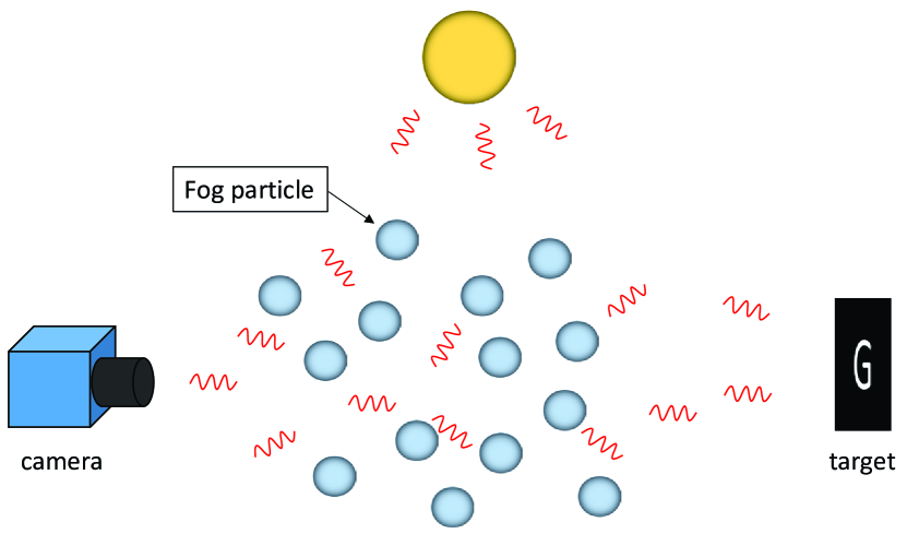
Figure 1: Setup of the McCartney model.

Recall that the scattering model proposed McCartney, including a scattering light model and an ambient light model, has the following expression [10]:

$$I\left(d,\lambda\right)=I_{0}\left(\lambda\right)e^{-\beta\left(\lambda\right)d}+I\left(\infty,\lambda\right)\left(1-e^{-\beta\left(\lambda\right)d}\right).$$ (1)

Here, $I\left(d,\lambda\right)$ represents the light measured by the camera, which corresponds to the image output by the camera. $d$ and $\lambda$ represent the distance from the object plane to the image plane and the wavelength, respectively. $I_{0}\left(\lambda\right)$ represents the light emitted or reflected by the object, which corresponds to the image without fog. $\beta\left(\lambda\right)$ represents the scattering coefficient. $I\left(\infty,\lambda\right)$ represents the ambient light, which corresponds to the noise. Notably, the fog image is a linear superposition of the scattering light (signal) and ambient light (noise).

The conceptual arrangement of our imaging technique based on a McCartney model is illustrated in Fig. 1. In the scattering light model, the irradiance of a single measurement event passed through a volume element with a unit cross-sectional area, a thickness of $dx$ and a period of time $dt$ can be expressed as

$$\frac{dI\left(x,\lambda,t\right)}{I\left(x,\lambda,t\right)}=-\beta\left(\lambda,t\right)dxdt,$$ (2)

where $\beta\left(\lambda,t\right)$ represents the time-dependent scattering coefficient. $x$ presents the vertical coordinate. By integrating Eq. 2, we obtain

$$I\left(d,\lambda,t\right)=\int_{t_{1}}^{t_{2}}I_{0}\left(\lambda,t\right)e^{-\beta\left(\lambda,t\right)d}dt,$$ (3)

where $\beta\left(\lambda,t\right)d$ denotes the optical path, and $\Delta t=t_{2}-t_{1}$ represents the integration time. We adopt a statistical view of light: a point source of radiation randomly emits photons in all possible directions [20]. Thus, the radiation measured during $\Delta t$ is the result of the superposition of a large number of photons or subfields. We have $\int_{\Delta t}I_{0}\left(\lambda,t\right)dt=\sum_{m=1}^{n}E_{m}\left(\lambda,t\right)$ with $E_{m}\left(\lambda,t\right)$ representing the $m$th photon or subfield, $n\propto\Delta t$. The measured light intensity, which is proportional to the number of photons, corresponds to the theoretical expectation [20], i.e.,

$$I\left(d,\lambda,t\right)=\sum_{m=1}^{n}E_{m}\left(\lambda,t\right)\int_{t_{1}}^{t_{2}}e^{-\beta\left(\lambda,t\right)d}dt,$$ (4)

In the ambient light model, the luminous intensity in volume $dv$ in the measurement direction is

$$dE\left(x,\lambda,t\right)=kx^{2}\beta\left(\lambda,t\right)d\omega dxdt,$$ (5)

where $dv=$ $d\omega x^{2}dx$, in which $d\omega$ is the solid angle from the lens to the target, and $k$ is a function related to the scattering type. Thus, the residual radiance obtained after scattering by the medium can be expressed as

$$dL\left(x,\lambda,t\right)=\frac{dE\left(x,\lambda,t\right)e^{-\beta\left(\lambda,t\right)x}}{x^{2}}.$$ (6)

We obtain the light intensity, i.e.,

$$dI\left(x,\lambda,t\right)=\frac{dL\left(x,\lambda,t\right)}{d\omega}.$$ (7)

Substituting Eq. 5 and Eq. 6 into Eq. 7, we obtain

$$dI\left(x,\lambda,t\right)=k\beta\left(\lambda,t\right)e^{-\beta\left(\lambda,t\right)x}dxdt.$$ (8)

The light intensity detected by the camera is obtained by integrating the above equation, i.e.,

$$I\left(d,\lambda,t\right)=k\sum_{m=1}^{n}E_{m}^{{}^{\prime}}\left(\lambda,t\right)\int_{t_{1}}^{t_{2}}\left(1-e^{-\beta\left(\lambda,t\right)d}\right)dt.$$ (9)

Practically, the scattering light and ambient light are simultaneously measured by the camera. Consequently, the fog image can be described as a linear superposition of the scattering light and ambient light, i.e.,

$$I\left(d,\lambda,t\right) =\sum_{m=1}^{n}E_{m}\left(\lambda,t\right)\int_{t_{1}}^{t_{2}}e^{-\beta\left(\lambda,t\right)d}dt$$

$$+\sum_{m=1}^{n}E_{m}^{{}^{\prime}}\left(\lambda,t\right)\int_{t_{1}}^{t_{2}}\left(1-e^{-\beta\left(\lambda,t\right)d}\right)dt$$ (10)

$$=S\left(d,\lambda,t\right)+A\left(d,\lambda,t\right).$$

Notably, both the scattering light and ambient light have photon number fluctuations, whether in one measurement event or in different measurement events.

A set of experimental results are used to demonstrate the above theory. The experimental setup is shown in Fig. 1. A quasi-monochromatic cosine LED with $\lambda=$528$\pm$10 nm illuminates an object (letter G), and then the reflected light is detected by a conventional camera (the imaging source is DFK23U618) through a time-variant fog medium with a length of 0.6 m. Fog is produced by 100% water. Fig. 2 shows that the photon number fluctuation is proportional to the integration time required for one measurement event. Moreover, the photon number fluctuation phenomenon is also significant for different measurement events. The quantitative results are shown in Fig. 3. The structural similarity (SSIM) and peak signal-to-noise ratio (PSNR) are used to present the photon number fluctuation results.

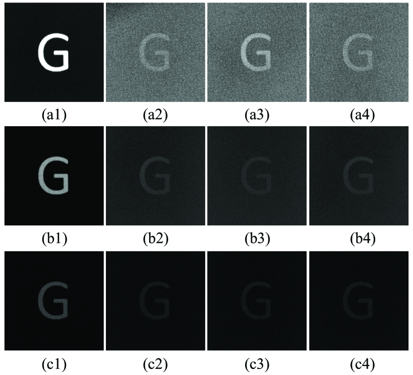
Figure 2: The images output by a conventional optical camera without fog (first column) and with fog (columns 2 to 4). The integration times are 1/30 second (top row), 1/50 second (middle row) and 1/150 second (bottom row).

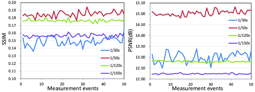
Figure 3: SSIM and PSNR curves produced for different integration times and different measurement events.

The photon number correlations between any two adjacent measurement events along the time axis are expressed as shown in [21]:

$$C\left(d,\lambda,t\right)=\left\langle I_{1}\left(d,\lambda,t_{1}\right)I_{2}\left(d,\lambda,t_{2}\right)\right\rangle.$$ (11)

To determine the result of Eq. 11, we consider the coherence time $\tau_{c}$ of the light field. Previous works showed that when $\tau_{c}>\Delta\tau$, where $\Delta\tau$ represents the time interval between two measurement events, we have that $\left\langle I_{1}I_{2}\right\rangle\neq 0$ [23-25]. Thus, Eq. 11 can be expressed as

$$C\left(d,\lambda,t\right) =\left\langle S_{1}\left(d,\lambda,t_{1}\right)S_{2}\left(d,\lambda,t_{2}\right)\right\rangle$$

$$+\left\langle A_{1}\left(d,\lambda,t_{1}\right)A_{2}\left(d,\lambda,t_{2}\right)\right\rangle.$$ (12)

The above result is still a linear superposition of signal and noise. If $\tau_{c}<\Delta\tau$, we have $\left\langle I_{1}I_{2}\right\rangle=0$ [22-24]. Thus, no image is obtained. Zerom et al. showed that $\left\langle I_{1}I_{2}\right\rangle\neq 0$ can be guaranteed by accumulating the intensity fluctuations of the light field at a certain time [24]. Nevertheless, the result is the same as Eq. 12.

Considering the photon number correlation between two adjacent measurement events of ambient light along the time axis, i.e.,

$$\left\langle A_{1}\left(d,\lambda,t_{1}\right)A_{2}\left(d,\lambda,t_{2}\right)\right\rangle=\left|G^{(1)}\left(t_{1},t_{2}\right)\right|^{2},$$ (13)

where $G^{(1)}$ is usually defined as the first-order coherence function [20]. If $\tau_{c}<\Delta\tau$, $G^{(1)}\left(t_{1},t_{2}\right)=0$. Consequently, this type of light does not have stable photon number correlation. Actually, the ambient photons randomly come from all possible directions and point sources. Moreover, due to the photon number accumulation, we have $\left\langle A_{1}A_{2}\right\rangle\rightarrow 0$ but $\left\langle A_{1}A_{2}\right\rangle\neq 0$.

The photon number correlation of scattering light can be expressed as

$$\left\langle S_{1}\left(d,\lambda,t_{1}\right)S_{2}\left(d,\lambda,t_{2}\right)\right\rangle=\left|G^{{}^{\prime}(1)}\left(t_{1},t_{2}\right)\right|^{2}.$$ (14)

Here, every point on the object can be seen as a point source that emits photon. These photons pass through the scattering medium and are focused onto an image plane by an imaging lens defined by the Gaussian thin lens equation $1/s_{o}+1/s_{i}=1/f,$ where $s_{o}$ is the distance between the object and the imaging lens, $s_{i}$ the distance between the imaging lens and the image plane, and $f$ the focal length of the imaging lens. Thus, scattering photons follow the point-point mapping relationship between the object plane and image plane. Due to the scattering of the medium, we have

$$0<\frac{\left\langle S_{1}\left(d,\lambda,t_{1}\right)S_{2}\left(d,\lambda,t_{2}\right)\right\rangle}{\left\langle S_{1}\left(d,\lambda,t_{1}\right)\right\rangle\left\langle S_{2}\left(d,\lambda,t_{2}\right)\right\rangle}<1.$$ (15)

Consequently, scattering light exhibits stable photon number correlation, even if photon number fluctuations still exist.

According to above analysis, if the measurement events meet the following conditions, i.e., (i) the measurement events can present spatial photon number fluctuations in time domain (i.e., $\left\langle I_{1}\right\rangle\neq\left\langle I_{2}\right\rangle$), and (ii) the time interval between two adjacent measurement events is larger than the coherence time of light field (i.e., $\left\langle S_{1}S_{2}\right\rangle\neq 0$, $\left\langle A_{1}A_{2}\right\rangle=0$). Eq. 12 can be expressed as

$$C\left(d,\lambda,t\right)=\left\langle S_{1}\left(d,\lambda,t_{1}\right)S_{2}\left(d,\lambda,t_{2}\right)\right\rangle.$$ (16)

Eq. 16 presents a fog-free image with low brightness. In practice, Eq. 12 is rewritten as

$$C\left(d,\lambda,t\right) =\left\langle S_{1}\left(d,\lambda,t_{1}\right)S_{2}\left(d,\lambda,t_{2}\right)\right\rangle$$

$$+\min\left\langle A_{1}\left(d,\lambda,t_{1}\right)A_{2}\left(d,\lambda,t_{2}\right)\right\rangle,$$ (17)

where $\min\left\langle A_{1}A_{2}\right\rangle$ represents $\left|\min\left\langle A_{1}A_{2}\right\rangle\right|\ll\left|\left\langle S_{1}S_{2}\right\rangle\right|$. Consequently, a high-quality defogging image can be reconstructed.

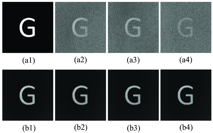
Figure 4: A set of fog images and reconstructed images. The integration time $\Delta t=1/30$ second. The time interval between two adjacent measurement events is $\Delta\tau=1$ second. The reconstructed image is obtained by measuring 20 fog images. (a1) The target image, (a2)-(a4) three fog images, and (b1)-(b4) a set of reconstructed images.

Figs. 4 and 5 are used to demonstrate Eq. 17. The experimental data are processed by the photon number correlation algorithm [25-28]. The results (Fig. 4) show that the influence of fog is almost completely eliminated. Additionally, the image brightness is slightly lower than that of the image without fog because the fluctuating photons are eliminated. The quantitative results (Fig. 5) show that the SSIM and PSNR values of the reconstructed images are much higher than those those of fog images, but SSIM$\neq 1$. The compared video is shown in supplemental material. Moreover, the quantitative comparison between our method and the defogging generative adversarial network is shown in Fig. 5 (for details, see supplemental material).

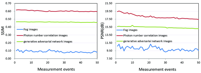
Figure 5: SSIM and PSNR curves of fog images and reconstructed images via photon number correlation and images via generative adversarial network.

Actually, the physical essence of measuring the photon number correlation in the time domain is to eliminate fluctuating photons through the fluctuating photons themselves. Consequently, a photon number fluctuation correlation algorithm is introduced to eliminate the fluctuating photon based on photon number fluctuation-fluctuation correlations [20,29,30]. First, the software records the registration time of each measurement event of a CCD camera element along the time axis. Then, the software calculates the average number of items per set: $\overline{p_{1}}$ and $\overline{p_{2}}$. Subsequently, the software classifies the values in each window as positive and negative fluctuations based on $\overline{p_{1}}$ and $\overline{p_{2}}$.

$$\Delta p_{j\alpha}^{\left(+\right)} =\left\{\begin{array}[c]{c}p_{j\alpha}-\overline{p_{j}},if,p_{j\alpha}>\overline{p_{j}}\\ 0,otherwise\end{array}\right.,$$ (20)

$$\Delta p_{j\alpha}^{\left(-\right)} =\left\{\begin{array}[c]{c}p_{j\alpha}-\overline{p_{j}},if,p_{j\alpha}<\overline{p_{j}}\\ 0,otherwise\end{array}\right.,$$ (23)

where $j=1,2$ labels two sets and $\alpha=1,2,...N$ labels the ath measurement. event. $N$ is the total size of each set. We define the following quantities:

$$\left(\Delta p_{1}\Delta p_{2}\right)_{\alpha}^{\left(++\right)} =\left|\left(\overline{p_{1}}-\Delta p_{1\alpha}^{(+)}\right)\left(\overline{p_{2}}-\Delta p_{2\alpha}^{(+)}\right)\right|,$$

$$\left(\Delta p_{1}\Delta p_{2}\right)_{\alpha}^{\left(--\right)} =\left|\left(\overline{p_{1}}-\Delta p_{1\alpha}^{(-)}\right)\left(\overline{p_{2}}-\Delta p_{2\alpha}^{(-)}\right)\right|,$$

$$\left(\Delta p_{1}\Delta p_{2}\right)_{\alpha}^{\left(+-\right)} =\left|\left(\overline{p_{1}}-\Delta p_{1\alpha}^{(+)}\right)\left(\overline{p_{2}}-\Delta p_{2\alpha}^{(-)}\right)\right|,$$

$$\left(\Delta p_{1}\Delta p_{2}\right)_{\alpha}^{\left(-+\right)} =\left|\left(\overline{p_{1}}-\Delta p_{1\alpha}^{(-)}\right)\left(\overline{p_{2}}-\Delta p_{2\alpha}^{(+)}\right)\right|.$$ (24)

The statistical average can be expressed as

$$\left\langle\Delta p_{1}\Delta p_{2}\right\rangle =\frac{1}{N}\sum_{\alpha=1}^{N}\left(\left(\Delta p_{1}\Delta p_{2}\right)_{\alpha}^{\left(++\right)}+\left(\Delta p_{1}\Delta p_{2}\right)_{\alpha}^{\left(--\right)}\right.$$

$$+\left.\left(\Delta p_{1}\Delta p_{2}\right)_{\alpha}^{\left(+-\right)}+\left(\Delta p_{1}\Delta p_{2}\right)_{\alpha}^{\left(-+\right)}\right).$$ (25)

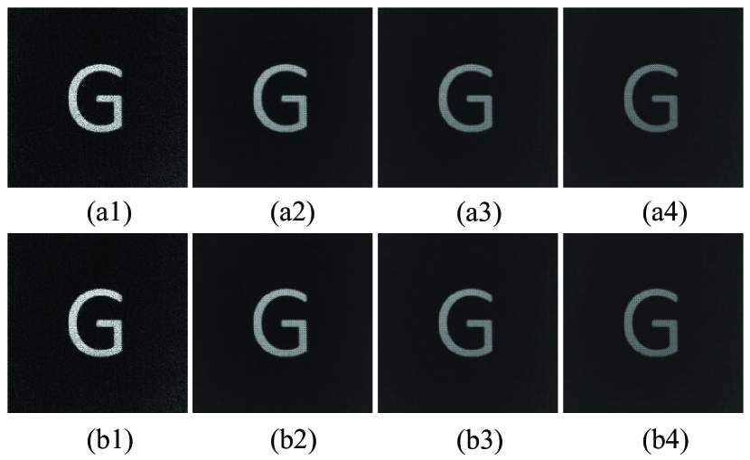
Figure 6: Top row: the images reconstructed by the photon number fluctuation correlation algorithm. The numbers of measurements are (a1) 10, (a2) 100, (a3) 200, and (a4) 300. Bottom row: the images reconstructed by the photon number correlation algorithm. The numbers of measurements are (b1) 10, (b2) 100, (b3) 200, and (b4) 300.

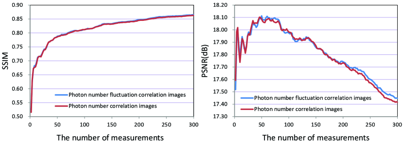
Figure 7: SSIM and PSNR curves of the images reconstructed by the photon number fluctuation correlation algorithm (blue) and the photon number correlation algorithm (red).

Fig. 6 compares the effects of the photon number fluctuation correlation algorithm and the photon number correlation algorithm. Quantitative comparisons between these two methods are shown in Fig. 7. If the selective attenuation of the light spectrum is ignored, the color of the target can be greatly restored in the defogging image. The simulation results obtained for color targets are shown in Fig. 8.

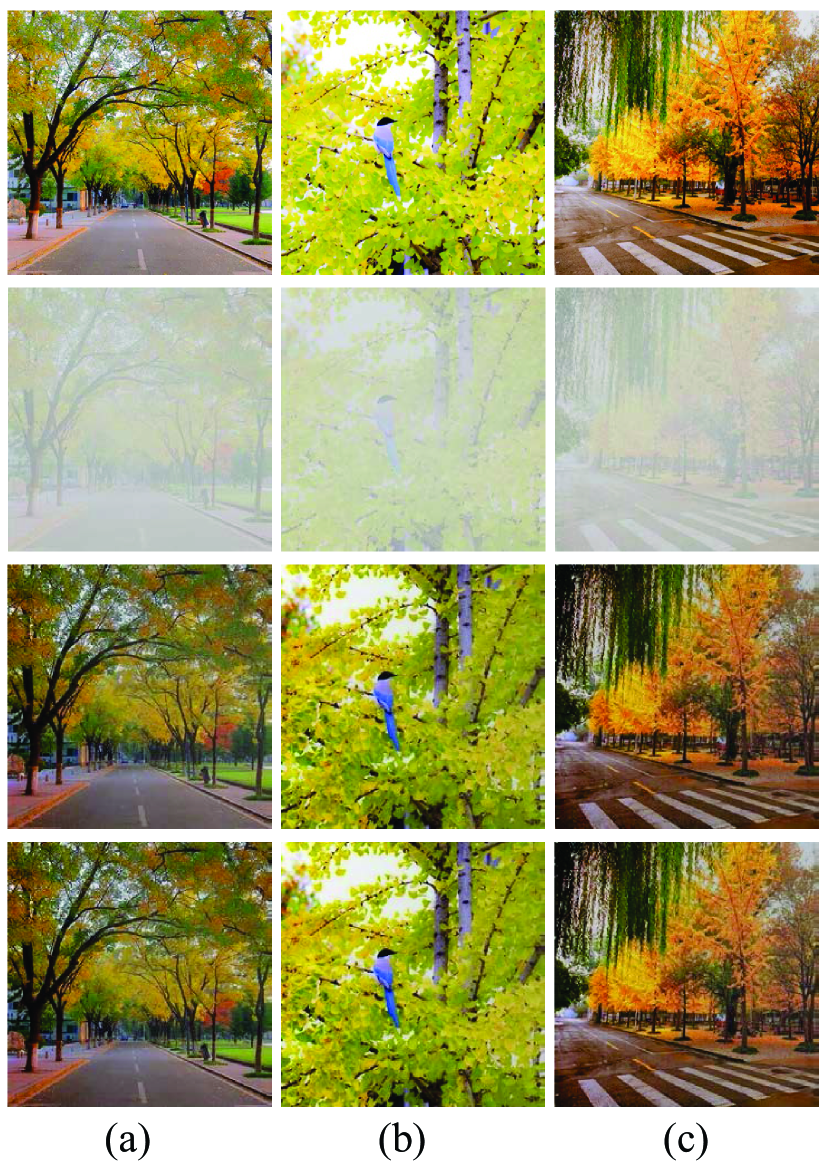
Figure 8: First row: three color targets. Second row: fog images. Third row: the images reconstructed by the photon number correlation algorithm. Fourth row: the images reconstructed by the photon number fluctuation correlation algorithm. The number of measurements is 50.

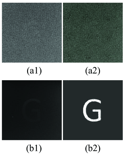
Figure 9: (a1) Indistinguishable fog image. The integration time $\Delta t=1/30$ second. (a2) The defogging image reconstructed by the cycle generative adversarial network. (b1) The image reconstructed by the photon number correlation algorithm with 80 measurements. Enlarge the images to obtain a more obvious effect. (b2) The image reconstructed by b1 with a generative adversarial network.

When the target is indistinguishable, a directly distinguishable image can be obtained by our methods, although the brightness of the reconstructed image is low (Fig. 9b1). However, distinguishing these low brightness images is not difficult for computer vision. Figure 9a2 shows that the target image cannot be recovered from the indistinguishable image by using a conventional defogging method with deep learning (for method, see supplemental material). However, a high-quality image (Fig. 9b2) can be recovered from the reconstructed defogging images by using deep learning method (for method, see supplemental material).

In summary, this article abandons the idea that fog is a scattering medium with space-time invariance, as assumed by the conventional McCartney model. The correlation properties of photons interacting with time-variant fog are studied. Our works show that the scattering photons and the ambient photons have different correlation properties in the time domain. Thus, a defogging image can be reconstructed by measuring this difference, which demonstrates that the time-variant nature of fog is a positive quantum resource. The only requirement is that software must be installed on the utilized imaging equipment to implement the defogging imaging function without changing any hardware.

This work was supported by the Natural Science Foundation of Shandong Province (ZR2022MF249) and the National Natural Science Foundation (12274257).

References

- (1) K.-M. He, J. Sun and X.-O. Tang, Single image haze removal using dark channel prior, IEEE Trans. Pattern Anal. Mach. Intell. 33(12): 2341-2353 (2010).
- (2) W.-Q. Ren, S. Liu, H. Zhang, J.-H. Pan, X.-C. Cao, and M.-H. Yang, Single image dehazing via multiscale convolutional neural networks, Eur. Conf. on Comput. Vis. pp: 154– 169. Springer, (2016).
- (3) B.-L. Cai, X.-M. Xu, K. Jia, C.-M. Qing, and D.-C. Tao, DehazeNet: An end-to-end system for single image haze removal, IEEE Trans. on Image Process. 25(11):5187–5198, (2016).
- (4) B.-Y. Li, X.-L. Peng, Z.-Y. Wang, J.-Z. Xu, and D. Feng, AOD-Net: All-in-one dehazing network, IEEE Int. Conf. on Comput. Vis. pp: 4770–4778, (2017).
- (5) D. Engin, A. Genc, H. Kemal Ekenel, Cycle-dehaze: Enhanced cyclegan for single image dehazing, Proc. IEEE Conf. Comput. Vis. Pattern Recog. pp: 8183-8192, (2018).
- (6) Z.-R. Zheng, W.-Q. Ren, X.-C. Cao, X.-B. Hu, T. Wang, F.-L. Song, and X.-Y. Jia, Ultra-high-definition image dehazing via multi-Guided bilateral learning, Proc. IEEE Conf. Comput. Vis. Pattern Recog. pp: 16185-16194 (2021).
- (7) X. Qin, Z.-L. Wang, Y.-C. Bai, X.-D. Xie, and H.-Z. Jia, FFA-Net: Feature fusion attention network for single image dehazing, Assoc. for Adv. Artif. Intell, pp: 11908–11915, (2020).
- (8) W.-Q. Ren, J.-S. Pan, H. Zhang, X.-C. Cao, and M.-H. Yang, Single image dehazing via multiscale convolutional neural networks with holistic edges. Int. J. Comput. Vision, 128(1): 240-259, (2020).
- (9) H.-Y. Wu, Y.-Y. Qu, S.-H. Lin, J. Zhou, R.-Z. Qiao, Z.-Z. Zhang, Y. Xie, and L.-Z. Ma, Contrastive learning for compact single image dehazing, Proc. IEEE Conf. Comput. Vis. Pattern Recog. pp:10551-10560, (2021).
- (10) E. J. McCartney, Optics of the atmosphere: scattering by molecules and particles, John Wiley and Sons, New York, 1976.
- (11) W.-L. Gong and S.-S. Han, Correlated imaging in scattering media, Opt. Lett. 36, 394-396 (2011).
- (12) M. Bina, D. Magatti, M. Molteni, A. Gatti, L. A. Lugiato, and F. Ferri, Backscattering Differential Ghost Imaging in Turbid Media, Phys. Rev. Lett. 110, 083901 (2013).
- (13) Z. Yang, L.-J. Zhao, X.-L. Zhao, W. Qin, and J.-L. Li, Lensless ghost imaging through the strongly scattering medium, Chin. Phys. B 25, 024202 (2016).
- (14) Q. Fu, Y.-F. Bai, X.-W. Huang, S.-Q. Nan, P.-Y. Xie, and X.-Q. Fu, Positive influence of the scattering medium on reflective ghost imaging, Photon. Res. 7, 1468-1472 (2019).
- (15) Y. Xiao, L.-N. Zhou and W. Chen, Experimental demonstration of ghost-imaging-based authentication in scattering media, Opt. Express 27, 20558-20566 (2019).
- (16) F.-Q. Li, M. Zhao, Z.-M. Tian, F. Willomitzer, and O. Cossairt, Compressive ghost imaging through scattering media with deep learning, Opt. Express 28(12), 17395-17408 (2020).
- (17) Z.-J. Gao, J.-H. Yin, Y.-F. Bai, and X.-Q. Fu, Imaging quality improvement of ghost imaging in scattering medium based on Hadamard modulated light field, Appl. Opt. 59, 8472-8477 (2020).
- (18) H. Liu, Y.-N. Chen, L. Zhang, D.-H. Li, and X.-W. Li, Color ghost imaging through the scattering media based on A-cGAN, Opt. Lett. 47, 569-572 (2022).
- (19) L.-X. Lin, J. Cao, D. Zhou, H. Cui, and Q. Hao, Ghost imaging through scattering medium by utilizing scattered light, Opt. Express 30, 11243-11253 (2022).
- (20) Y. Shih, The physics of turbulence-free ghost imaging, Technologies, 4(4): 39 (2016).
- (21) H. Yu, R.-H. Lu, S.-S. Han, H.-L. Xie, G.-H. Du, T.-Q. Xia, D.-M. Zhu, Fourier-transform ghost imaging with hard X rays, Phys. Rev. Lett. 117: 113901, (2016).
- (22) X.-F. liu, X.-H. Chen, X.-R. Yao, W.-K. Yu, G.-J. Zhai, L.-A. Wu, Lensless ghost imagin with sunlight, Opt. Lett. 39(8): 2314-2317 (2014).
- (23) M.-F. Li, L. Yan, R. Yang, J. Kou, and Y.-S. Liu, Turbulence-free intensity fluctuation self-correlation imaging with sunlight, Acta Phys. Sin 68(9): 094204 (2019).
- (24) P. Zerom, Z. Shi, M. N. O’Sullivan, K. W. C. Chan, M. Krogstad, Thermal ghost imaging with averaged speckle patterns, Phys. Rev. A 86(6):063817 (2012).
- (25) R. Hanbury Brown, R. Q. Twiss, Correlation between photons in two coherent beams of light, Nature 177(4497): 27-29 (1956).
- (26) T. B. Pittman, Y. H. Shih, D. V. Strekalov, and A. V. Sergienko, Optical imaging by means of two-photon quantum entanglement, Phys. Rev. A 52, R3429 (1995).
- (27) D. Pelliccia, A. Rack, M. Scheel, V. Cantelli, and D. M. Paganin, Experimental X-ray ghost imaging, Phys. Rev. Lett. 117, 219902 (2016).
- (28) Z.-J. Tan, H. Yu, R.-G. Zhu, R.-H. Lu, S.-S. Han, C.-F. Xue, S.-M. Yang, and Y.-Q. Wu, Single-exposure Fourier-transform ghost imaging based on spatial correlation, Phys. Rev. A 106, 053521 (2022).
- (29) H. Chen, T. Peng, and Y. Shih, 100% correlation of chaotic thermal light, Phys. Rev. A 88, 023808 (2013).
- (30) T. A. Smith and Y. Shih, Turbulence-free double-slit interferometer, Phys. Rev. Lett. 120, 063606 (2018).