On the Role of Attention in Prompt-tuning

Abstract

Prompt-tuning is an emerging strategy to adapt large language models (LLM) to downstream tasks by learning a (soft-)prompt parameter from data. Despite its success in LLMs, there is limited theoretical understanding of the power of prompt-tuning and the role of the attention mechanism in prompting. In this work, we explore prompt-tuning for one-layer attention architectures and study contextual mixture-models where each input token belongs to a context-relevant or -irrelevant set. We isolate the role of prompt-tuning through a self-contained prompt-attention model. Our contributions are as follows: (1) We show that softmax-prompt-attention is provably more expressive than softmax-self-attention and linear-prompt-attention under our contextual data model. (2) We analyze the initial trajectory of gradient descent and show that it learns the prompt and prediction head with near-optimal sample complexity and demonstrate how the prompt can provably attend to sparse context-relevant tokens. (3) Assuming a known prompt but an unknown prediction head, we characterize the exact finite sample performance of prompt-attention which reveals the fundamental performance limits and the precise benefit of the context information. We also provide experiments that verify our theoretical insights on real datasets and demonstrate how prompt-tuning enables the model to attend to context-relevant information.

1 Introduction

Transformer models have achieved remarkable success in a wide array of machine learning domains spanning language modeling, vision, and decision making. Recently, one of the key techniques that has helped pave the way for the deployment of transformers to ever increasing application areas is their ability to adapt to multiple unseen tasks by conditioning their predictions through their inputs – a technique known as prompt-tuning (lester2021power; li2021prefix). Concretely, prompt-tuning provides a more efficient (cheaper/faster) alternative to fine-tuning the entire weights of the transformer by instead training (fewer) so-called prompt parameters that are appended on the input and can be thought of as an input interface. In fact, several recent works have demonstrated experimentally that prompt-tuning is not only more efficient, but often even becomes competitive to fine-tuning in terms of accuracy (lester2021power; liu2023pre). However, there is currently limited formal justification of such observations. This motivates the first question of this paper:

How does prompt-tuning compare to fine-tuning in terms of expressive power? Are there scenarios prompt-tuning outperforms fine-tuning in that regard?

The core constituent of a transformer, and thus of prompt-tuning, is the attention mechanism. Through the attention layer, prompts get to interact with other input features, create/modify attention weights, and facilitate the model to attend on latent task-specific information. The standard attention layer relies on softmax nonlinearities. Operationally, the softmax function allows a model to selectively focus on certain parts of the input tokens when generating attention outputs. However, there is little rigorous understanding of attention-based prompt-tuning. Concretely,

What is the role of the softmax-attention in prompt-tuning in terms of optimization and generalization? How does it locate and extract relevant contextual information?

Contributions. Our contributions are as follows:

• We show that a particular form of attention which we refer to as prompt-attention naturally arises from the self-attention model with prompt-tuning. We identify provable scenarios where it is more expressive than self-attention and linear-prompt-attention. This separation result reveals insightful data models where prompt-tuning can be superior to fine-tuning with self-attention.

• We develop new statistical foundations for gradient-based prompt-tuning: we study the optimization and generalization dynamics of the initial trajectory of gradient descent for optimizing prompt-attention. Concretely, we show the first few iterations learn the prompt and prediction head with near-optimal sample complexity while achieving high accuracy.

• Our results provide insights into the critical role of softmax in facilitating attention: we show how the initial trajectory of gradient descent utilizes softmax to provably attend to sparse context-relevant tokens, ignoring noisy/nuisance tokens.

• We also characterize the exact finite sample performance of prompt-attention assuming known prompt but unknown prediction head. This reveals the fundamental performance limits and precisely quantifies the benefits of context information.

• Our results highlight various trade-offs among different model parameters: (i) the role of sparsity, i.e., the fraction of context-relevant tokens, and (ii) the relative effects of the different constituents of context-relevant tokens.

• Finally, we empirically validate our theoretical insights on both synthetic contextual-mixture datasets and image-classification datasets. Specifically, we compare multiple variants of prompt-tuning against standard fine-tuning on the latter. Our results highlight the role of prompt-attention in selecting relevant tokens in the image classification setting.

Related works.

Attention, specifically the so-called self-attention, is the backbone mechanism of transformers (vaswani2017attention). It differs from conventional models (e.g., multi-layer perceptrons and convolutional neural networks) in that it computes feature representations by globally modeling interactions between different parts of an input sequence. Despite tremendous empirical success (see, e.g., vaswani2017attention; brown2020language; saharia2022photorealistic; ramesh2022hierarchical; chatgpt; narayanan2021efficient; reed2022generalist, and references therein), the underlying mechanisms of the attention layer remain largely unknown: How does it learn? What makes it better (and when) compared to conventional architectures? Yun2020Are show that self-attention based transformers with large enough depth are universal approximators of seq2seq functions. Focusing on the self-attention component, edelman2021inductive show that self-attention can efficiently represent sparse functions of its input space, while sahiner2022unraveling; ergen2022convexifying analyze convex-relaxations of Self-attention, and baldi2022quarks; dong2021attention study the expressive ability of attention layers. However, these works do not characterize the optimization and generalization dynamics of attention. To the best of our knowledge, the only prior works attempting this are jelassi2022vision and ICLRsub2022. jelassi2022vision assume a simplified attention structure in which the attention matrix is not directly parameterized in terms of the input sequence. Our paper also distinguishes itself from contemporaneous work by ICLRsub2022 in several ways: (1) Unlike their data model, ours incorporates a context vector and employs a sub-Gaussian noise model instead of assuming bounded noise. (2) We provide a precise asymptotic analysis that elucidates the role of various problem parameters. (3) While ICLRsub2022 primarily focuses on vanilla self-attention, our study centers on understanding the potential benefits of prompt-tuning through prompt-attention.

2 Problem setting

2.1 Motivation: Prompt-tuning

Consider a single-head self-attention layer

$$\bm{O}_{\text{pre}}=\phi({\bm{X}}\bm{W}_{Q}\bm{W}_{K}^{\top}{\bm{X}}^{\top}){\bm{X}}\bm{W}_{V}\,,$$ (1)

with input ${\bm{X}}\in\mathbb{R}^{T\times d}$ consisting of $T$ tokens of dimension $d$ each, trainable parameters $(\bm{W}_{K},\bm{W}_{Q},\bm{W}_{V})$ and a softmax nonlinearity $\phi:\mathbb{R}^{T}\mapsto\mathbb{R}^{T}$, $[\phi({\bm{v}})]_{t}=e^{v_{t}}/\sum_{t^{\prime}\in[T]}e^{v_{t^{\prime}}}$ that acts row-wise when its argument is a $T\times T$ matrix. We scalarize the output of the self-attention layer with a trainable linear head $\bar{\bm{U}}$ which yields

$$y_{\text{pre}}=\langle\bar{\bm{U}},\bm{O}_{\text{pre}}\rangle=\langle\bm{U},\phi({\bm{X}}\bm{W}_{Q}\bm{W}_{K}^{\top}{\bm{X}}^{\top}){\bm{X}}\rangle\,.$$ (2)

Note here that we implicitly subsume the value matrix $\bm{W}_{V}$ in the linear head via $\bm{U}:=\bar{\bm{U}}\bm{W}_{V}^{\top}$.

We assume that the model above is pre-trained so that $\bm{W}_{K},\bm{W}_{Q},\bm{U}$ are fixed. Our goal is to use the pretrained transformer on (potentially) new classification tasks. Towards this goal, we explore the use of prompt-tuning, introduced in li2021prefix; lester2021power as an alternative to fine-tuning the existing transformer weights.

Prompt-tuning appends a trainable prompt ${\bm{P}}\in\mathbb{R}^{m\times d}$ to the input features ${\bm{X}}\in\mathbb{R}^{T\times d}$ with the goal of conditioning the transformer to solve the new classification task. Let ${\bm{X}}_{{\bm{P}}}:=\begin{bmatrix}{\bm{P}}\\ {\bm{X}}\end{bmatrix}\in\mathbb{R}^{(T+m)\times d}$ be the new transformer input. The output of the attention-layer is thus is of the form

$$\bm{O}=\phi({\bm{X}}_{{\bm{P}}}\bm{W}_{Q}\bm{W}_{K}^{\top}{\bm{X}}^{\top}){\bm{X}}.$$

Note that this is slightly different from (1) in that now the layer computes a cross-attention between the augmented inputs ${\bm{X}}_{{\bm{P}}}$ and the original inputs ${\bm{X}}$. This is also equivalent to self-attention on ${\bm{X}}_{{\bm{P}}}$ after masking the prompt ${\bm{P}}$ from keys. This masking is used to cleanly isolate the residual contribution of the prompt without impacting the frozen attention output. Concretely, let $\bm{W}_{\text{head}}$ be the prediction head associated with the prompt tokens. As before, we scalarize the output by projecting with a linear head of size $(T+m)\times d$ as follows:

$$y=\langle[{\bm{W}_{\text{head}}}^{\top}~{}\bm{U}^{\top}]^{\top},\phi({\bm{X}}_{{\bm{P}}}\bm{W}_{Q}\bm{W}_{K}^{\top}{\bm{X}}^{\top}){\bm{X}}\rangle$$ (3)

$$=\underbrace{\langle{\bm{W}_{\text{head}}},\phi({\bm{P}}\bm{W}_{Q}\bm{W}_{K}^{\top}{\bm{X}}^{\top}){\bm{X}}\rangle}_{\text{prompt-attention $y_{\text{new}}$}}+\underbrace{\langle\bm{U},\phi({\bm{X}}\bm{W}_{Q}\bm{W}_{K}^{\top}{\bm{X}}^{\top}){\bm{X}}\rangle}_{\text{frozen self-attention $y_{\text{pre}}$}}.$$

Here, $y_{\text{new}}$ captures the additive impact of prompt-tuning on the prediction. We denote the trainable parameters in the model above as $\bm{\theta}:=({\bm{W}_{\text{head}}},{\bm{P}})$ Since the $y_{\text{new}}$ term becomes a self-contained module and the features attend directly to the prompt vector, we will refer to it as prompt-attention.

Our goal is understanding the expressivity, training dynamics, and generalization properties of the above model. To simplify our analysis, we consider the following setting.

1. We focus our attention on the novel component $y_{\text{new}}$ of the model output in (3) so as to isolate and fully understand the capabilities of prompt-attention.

2. We assume $\bm{W}_{K},\bm{W}_{Q}\in\mathbb{R}^{d\times d}$ are full-rank.

3. We assume a single trainable prompt ${\bm{q}}\in\mathbb{R}^{d}$ i.e., $m=1$.

Prompt-attention model. Using these assumptions and setting ${\bm{q}}:=\bm{W}_{K}\bm{W}_{Q}^{\top}{\bm{P}}^{\top}\in\mathbb{R}^{d}$ and ${\bm{w}}={\bm{W}_{\text{head}}^{\top}}\in\mathbb{R}^{d}$, we arrive at our core prompt-attention model $f^{\textsc{att}}_{\bm{\theta}}$ (or simply $f^{\textsc{att}}$):

$$f^{\textsc{att}}_{\bm{\theta}}({\bm{X}})=\langle{\bm{w}},{\bm{X}}^{\top}\phi\left({\bm{X}}{\bm{q}}\right)\rangle,~{}\bm{\theta}=({\bm{w}},{\bm{q}}).$$ (4)

We shall see that this model exhibits interesting properties to learn rich contextual relationships within the data and can even be more expressive than a single self-attention layer.

We remark that the model above is of interest even beyond the context of prompting: the prompt-attention model in (4) is reminiscent of the simplified model proposed in earlier seq2seq architectures (bahdanau2014neural; xu2015show; chan2015listen) preceding self-attention and Transformers (vaswani2017attention). Indeed, in the simplified attention mechanism of (bahdanau2014neural; xu2015show; chan2015listen), the tokens’ relevance scores and corresponding attention weights are determined by $\bm{a}=\phi({\bm{X}}{\bm{q}})$ in which ${\bm{q}}$ is a trainable vector and $\phi$ is the softmax-score transformation. Note here that the trainable parameter ${\bm{q}}$ corresponds exactly to the trainable prompt vector in (4).

2.2 Contextual data model

Consider supervised classification on IID data $({\bm{X}},y)\sim\mathcal{D}$ with features ${\bm{X}}\in\mathbb{R}^{T\times d}$ and binary label $y\in\{\pm 1\}$.

Dataset model. We assume the following about an example $({\bm{X}},y)$ drawn from $\mathcal{D}$: The labels $y$ are distributed as $\mathbb{P}(y=1)=1-\mathbb{P}(y=-1)=\pi$; for simplicity, we set $\pi=1/2$ so that $\mathbb{E}[y]=0$. The tokens $\bm{x}_{t},t\in[T]$ of input example ${\bm{X}}:=[\bm{x}_{1},\ldots,\bm{x}_{T}]$ are split into a context-relevant set $\mathcal{R}\subset[T]$ and context-irrelevant set $\mathcal{R}^{c}:=[T]-\mathcal{R}$. Specifically, conditioned on the labels and relevance set $\mathcal{R}$, tokens $\bm{x}_{t},t\in[T]$ within ${\bm{X}}$ are i.i.d. as follows

$$\bm{x}_{t}|y=\begin{cases}{\bm{q}}_{\star}+y{\bm{w}}_{\star},&t\in\mathcal{R}~{}~{}~{}~{}~{}~{}\text{(relevant token)}\\ -\delta^{q}{\bm{q}}_{\star}-\delta^{w}y{\bm{w}}_{\star}+\bm{z}_{t},&t\not\in\mathcal{R}~{}~{}~{}~{}~{}~{}\text{({ir}relevant token)}\,.\end{cases}$$ (DATA)

In the above, ${\bm{q}}_{\star}$ is a context-vector that indicates token relevance and ${\bm{w}}_{\star}$ is a regressor vector. $y,\delta:=(\delta^{q},\delta^{w}),(\bm{z}_{t})_{t=1}^{T}$ are independent variables as follows:

• $\delta=(\delta^{q},\delta^{w})\in\mathbb{R}^{2}$ is a bounded random variable that obeys $\delta^{q}\geq 0$. Thus, $\delta$ reflects out-of-context information within irrelevant tokens. However, $\delta$ is allowed to expose label information through $\delta^{w}$. When $\delta=(0,0)$ almost surely, we call the resulting distribution core dataset model.

• $\bm{z}_{t}$ are independent centered subgaussian and random variables with covariance $\bm{\Sigma}$ (see Ass. 1.a). When $\bm{\Sigma}=0$, we call the resulting distribution discrete dataset model.

• We allow the relevance set $\mathcal{R}$ to be non-stochastic. This includes $\mathcal{R}$ being adversarial to the classification model.

• We assume constant fraction $\zeta=|\mathcal{R}|/T\in(0,1)$ of label-relevant tokens for each input example ${\bm{X}}$ drawn from $\mathcal{D}$. Thus, $\zeta$ represents the sparsity of relevant signal tokens.

Training dataset ${\mathcal{S}}:=({\bm{X}}_{i},y_{i})_{i=1}^{n}$. We draw $n$ i.i.d. samples from $\mathcal{D}$ to form our training dataset ${\mathcal{S}}:=({\bm{X}}_{i},y_{i})_{i=1}^{n}$. For $i$’th example $({\bm{X}}_{i},y_{i})$, we denote the tokens by $(\bm{x}_{i,t})_{t=1}^{T}$, noise by $(\bm{z}_{i,t})_{t=1}^{T}$, relevance set by $\mathcal{R}_{i}$, and out-of-context variable by $\delta_{i}=(\delta^{q}_{i},\delta^{w}_{i})$.

Ideally, for $i$’th example, we would like to identify its context-relevant set $\mathcal{R}_{i}$ and discard the rest. This would especially help when the signal-to-noise-ratio is small, i.e. $\zeta=|\mathcal{R}_{i}|/T\ll 1$. This is precisely the role of the context-vector ${\bm{q}}_{\star}$: Observe that, per our construction, relevant tokens have positive correlation with ${\bm{q}}_{\star}$ whereas irrelevant tokens have non-positive correlation with ${\bm{q}}_{\star}$ in expectation. Thus, by focusing attention onto tokens based on their ${\bm{q}}_{\star}$ correlation, we can potentially select the relevant set.

Remark 1 (Model interpretation).

(DATA) can be thought of as a simplified model for binary image classification with tokens being image patches of two types: ones revealing information about the label (set $\mathcal{R}$) and uninformative ones containing noise. Tokens in $\mathcal{R}$ contain information indicating: (i) class-membership via signed-regressor $y{\bm{w}}_{\star}$ and (ii) context-relevance via context-vector ${\bm{q}}_{\star}$. The signed-regressor differs across tokens of examples belonging to different classes $y\in\{\pm 1\}$, while the context-vector is common for all context-relevant tokes across classes. For a concrete example, consider images each depicting multiple, say $|\mathcal{R}|$, birds of one type surrounded by label-irrelevant/noisy background. The goal is to classify images according to one of two types of birds. Here, think of “context” as feature-information indicating corresponding pixels belong to “bird” (of either type) rather than “background,” while the “regressor” represents feature information useful to distinguish between two bird types. Alternatively, (DATA) may be modeling deep representations (rather than raw pixels) of the original images. Overall, simplified models similar to (DATA) have been used previously to analyze optimization and generalization dynamics of training fully-connected (frei2022random) and convolutional models (cao2022benign). Specifically, (DATA) is an extension of the commonly used (sub)-Gaussian mixture model customized to the nature of attention: each example is tokenized and context-relevant information is described in terms of both a regressor (differing between classes) and a context (common across classes).

2.3 Baseline Models

We compare performance of the prompt-attention model in (4) with the following three baseline models.

The linear model is parameterized by $\bm{\theta}={\bm{w}}$ and outputs

$$f^{\textsc{lin}}({\bm{w}})=\frac{1}{T}{\bm{w}}^{\top}{\bm{X}}^{\top}\mathds{1}_{T}=\frac{1}{T}\sum\nolimits_{t\in[T]}{\bm{w}}^{\top}\bm{x}_{t}.$$ (5)

Note this corresponds to a prompt-attention model with uniform attention weights $[\bm{a}]_{t}=1/T,t\in[T].$

The self-attention model is a strict generalization of the linear model. Recalling (2), let us merge the key-query weights $\bm{W}:=\bm{W}_{Q}\bm{W}_{K}^{\top}$ (without losing generality) and gather weights into $\bm{\theta}=(\bm{U},\bm{W})$; We then write it as

$$f^{\textsc{satt}}(\bm{U},\bm{W})=\frac{1}{T}\left<\bm{U},\phi({\bm{X}}\bm{W}{\bm{X}}^{\top}){\bm{X}}\right>.$$ (6)

Rather than using a $Td$ dimensional $\bm{U}$, we will also consider the simpler token-pooling via $\bm{U}=\mathds{1}_{T}\bm{u}^{\top}$ for $\bm{u}\in\mathbb{R}^{d}$.

The linear-attention model parameterized by $\bm{\theta}=({\bm{w}},{\bm{q}})$ replaces the softmax score transformation in (4) with a linear function and outputs

$$f^{\textsc{lin-att}}({\bm{w}},{\bm{q}})={\bm{w}}^{\top}{\bm{X}}^{\top}{\bm{X}}{\bm{q}}/T.$$ (7)

2.4 Training

Given ${\mathcal{S}}=({\bm{X}}_{i},y_{i})_{i=1}^{n}$ drawn i.i.d. from $\mathcal{D}$, we solve square-loss empirical risk minimization to obtain $\bm{\hat{\theta}}=({\hat{\bm{w}}},{\bm{\hat{q}}})$

$$\bm{\hat{\theta}}=\arg\min_{\bm{\theta}}\widehat{\mathcal{L}}_{{\mathcal{S}}}(\bm{\theta}):=\frac{1}{2n}\sum_{i=1}^{n}(y_{i}-f_{\bm{\theta}}({\bm{X}}_{i}))^{2}.$$ (8)

Within our theoretical investigation, we are interested in the following performance criteria for models $f\in\{f^{\textsc{att}},f^{\textsc{lin-att}},f^{\textsc{satt}}\}$:

• Classification error: For a model $f_{\bm{\hat{\theta}}}$ this is defined as $\textsc{err}(\bm{\hat{\theta}}):=\mathbb{P}(yf_{\bm{\hat{\theta}}}({\bm{X}})<0)$.

• Test risk: $\mathcal{L}(\bm{\hat{\theta}})=\mathbb{E}_{(y,{\bm{X}})\sim\mathcal{D}}[(y-f_{\bm{\hat{\theta}}}({\bm{X}}))^{2}]$.

2.5 Assumptions and notations

First, we formally state our assumptions on the noisy tokens. The more general condition is that noise is subgaussian and satisfies a mild zero third-moment condition.

Assumption 1.a.

The noise vector $\bm{z}\sim{\mathcal{S}}\mathcal{N}(\sigma)$ is centered $\sigma$-subGaussian, i.e. $\|\bm{z}\|_{\psi_{2}}=\sigma$. Moreover, its distribution is symmetric and has zero-third moment, i.e. $\mathbb{E}\Big{[}\bm{z}\otimes\left(\bm{z}^{\top}\bm{z}\right)\Big{]}=0$. Let $\bm{\Sigma}:=\mathbb{E}[\bm{z}\bm{z}^{\top}]$ denote the noise covariance.

For some of our results it will be convenient to further assume that noise is Gaussian since this leads to precise formulas that are easily interpretable.

Assumption 1.b.

The noise vector $\bm{z}\sim\mathcal{N}(0,\sigma^{2}\mathds{I})$ is isotropic Gaussian with variance $\sigma^{2}.$

Second, we require a mild assumption on the correlation between the context ${\bm{q}}_{\star}$ and classifier ${\bm{w}}_{\star}$ to guarantee that pure signal tokens ${\bm{q}}_{\star}+y{\bm{w}}_{\star}$ are correctly classified by the true regressor ${\bm{w}}_{\star},$ i.e. $y{\bm{w}}_{\star}^{\top}({\bm{q}}_{\star}+y{\bm{w}}_{\star})>0$. For convenience, we denote

$$W:=\|{\bm{w}}_{\star}\|,~{}~{}~{}Q:=\|{\bm{q}}_{\star}\|,~{}~{}~{}\rho:={{\bm{q}}_{\star}^{\top}{\bm{w}}_{\star}}/{(\|{\bm{q}}_{\star}\|\|{\bm{w}}_{\star}\|)}.$$

Assumption 3.a.

Correlation satisfies $\left\lvert\rho\right\rvert<{W}/{Q}.$

We will also often consider the special case of zero correlation $\rho$ and thus state it as separate assumption below. This orthogonality assumption, is useful for more tractable analysis as it helps decouple feature selection and prediction.

Assumption 3.b.

The context and classifier vectors are orthogonal, i.e. ${\bm{q}}_{\star}\perp{\bm{w}}_{\star}$.

Notation.  We use boldface letters for vectors and matrices. $\mathds{1}_{m}$ represents an $m$-dimensional all-ones vector. For a vector ${\bm{v}}$, $\|{\bm{v}}\|$ denotes its Euclidean norm and ${\bm{v}}/\|{\bm{v}}\|$ its normalization. $\phi(\cdot)$ denotes the softmax transformation. $\mathcal{Q}(\cdot)$ denotes the tail function of the standard normal distribution. $\,\wedge\,$ and $\,\vee\,$ denote the minimum and maximum of two numbers, respectively. ${\tilde{\mathcal{O}}}()$ and $\gtrsim$ notations suppress logarithmic dependencies. Finally, $\propto$ denotes proportionality.

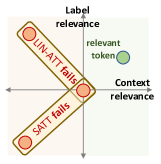
(a) Failure modes

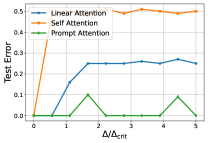
(b) Varying $\Delta$ with $\delta_{q}=\delta_{w}$

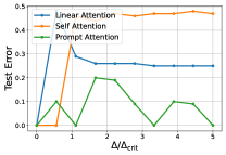
(c) Varying $\Delta$ with $\delta_{q}=-\delta_{w}$

Figure 1: This figure summarizes and verifies the outcomes of Theorem 1. Fig (a) depicts the outcome of our Theorem 1. Relevant token is at position $y{\bm{w}}_{\star}+{\bm{q}}_{\star}$ whereas red tokens (irrelevant) are in positions $-\delta({\bm{q}}_{\star}\pm y{\bm{w}}_{\star})$ with $\delta\in\{0,\Delta\}$. Figures (b) & (c) plot the performance of our attention models under the contextual dataset with $\delta$ equally-likely over $\{0,\Delta\}$ for a synthetic setup (cf. Section LABEL:sec:exp-synthetic). We set $n=100$, $d=T=10$, $\zeta=0.4$ and train with 100 SGD epochs. We report the median test accuracy over 20 trials. Fig (b) sets $\delta=\delta_{q}=\delta_{w}$ and verifies self-attention has $\geq 50\%$ error (for $\Delta\geq\Delta_{\text{crit}}{=(1-\zeta)^{-2}}$). Fig (c) sets $\delta=\delta_{q}=-\delta_{w}$ and verifies linear-prompt-attention has $\geq 25\%$ error (when $\delta\geq\Delta_{\text{crit}}=\sqrt{\zeta/(1-\zeta)}$ in this case).

3 Contrasting prompt-attention to baselines

In this section, we establish separation results between prompt-attention (cf. (4)) and the baselines of self-attention (cf. (6)) and linear attention (cf. (7)). For this, we focus on the discrete dataset model with noiseless irrelevant tokens ($\bm{z}_{t}=0,t\in[T]$).

We first observe that if $\delta=(\delta^{q},\delta^{w})$ admits a single value, even a linear model can solve the discrete dataset model.

Observation 1 (Linear model solves singleton).

Suppose $(\delta^{q},\delta^{w})=(\Delta^{q},\Delta^{w})$ almost surely for $\Delta^{q},\Delta^{w}\in\mathbb{R}$. Set ${\bm{w}}_{\star}^{\prime}=(\bm{I}-\bar{{\bm{q}}}_{\star}\bar{{\bm{q}}}_{\star}^{\top}){\bm{w}}_{\star}$. As long as $\Delta^{w}\neq\zeta/(1-\zeta)$ and ${\bm{w}}_{\star}^{\prime}\neq 0$, $f^{\textsc{lin}}({\bm{w}}_{\star}^{\prime})$ or $f^{\textsc{lin}}(-{\bm{w}}_{\star}^{\prime})$ achieves perfect accuracy.

Thus, to investigate the expressivity of $f^{\textsc{att}},f^{\textsc{satt}},f^{\textsc{lin}}$, $(\delta^{q},\delta^{w})$ would need to admit two or more values. Perhaps surprisingly, we prove that, as soon as, $(\delta^{q},\delta^{w})$ comes from a binary distribution, then both $f^{\textsc{satt}}$ and $f^{\textsc{lin}}$ can indeed provably fail. Importantly, this happens in the regime $\delta^{q}\geq 0$ where prompt-attention thrives.

Theorem 1 (Separation of population accuracies).

Consider the discrete dataset model where we set $\bm{\Sigma}=0$ in (DATA). The following statements hold:

1. Prompt-attention: Suppose $\rho^{2}<1$, $\delta^{q}\geq 0$, and $|\delta^{w}|\leq C$ almost surely. Define ${\bm{q}}_{\star}^{\prime}=(\bm{I}-\bar{{\bm{w}}}_{\star}\bar{{\bm{w}}}_{\star}^{\top}){\bm{q}}_{\star},{\bm{w}}_{\star}^{\prime}=(\bm{I}-\bar{{\bm{q}}}_{\star}\bar{{\bm{q}}}_{\star}^{\top}){\bm{w}}_{\star}$. For $\Gamma>\frac{\log({C(1/\zeta-1)})}{Q^{2}(1-\rho^{2})}$, choosing $\bm{\theta}=({\bm{w}}_{\star}^{\prime},\Gamma{\bm{q}}_{\star}^{\prime})$, $f^{\textsc{att}}_{\bm{\theta}}$ achieves perfect classification accuracy on (DATA).

2. Self-attention: In (DATA), choose $(\delta^{q},\delta^{w})$ to be $(0,0)$ or $({\Delta,\Delta})$ equally-likely with $\Delta>(1-\zeta)^{-2}$.

• For any choice of $(\bm{U}=\mathds{1}\bm{u}^{\top},\bm{W})$, $f^{\textsc{satt}}(\mathds{1}\bm{u}^{\top},\bm{W})$ achieves 50% accuracy (i.e. random guess).

• For any choice of $(\bm{U},\bm{W})$, there exists a (DATA) distribution with adversarial relevance set choices such that $f^{\textsc{satt}}(\bm{U},\bm{W})$ achieves 50% accuracy.

3. Linear-attention: In (DATA), choose $(\delta^{q},\delta^{w})$ to be $(0,0)$ or $({\Delta,-\Delta})$ equally-likely with $\Delta>\sqrt{\zeta/(1-\zeta)}$. For any choice of $({\bm{w}},{\bm{q}})$, $f^{\textsc{lin-att}}({\bm{w}},{\bm{q}})$ achieves at most 75% accuracy.

See Fig. 1 for an illustration of the main takeaways from Thm. 1 and a numerical validation of its conclusion on synthetic data. While surprising, the reason prompt-attention can provably beat self-attention is because it is optimized for context-retrieval and can attend perfectly on the relevant contextual information. In contrast, self-attention scores are fully feature-based; thus, context information is mixed with other features and can be lost during aggregation of the output. Also note that all results, with the exception of self-attention for general $\bm{U}$, hold for arbitrary choices of the relevance sets (including adversarial ones). The reason is that tokens are pooled and the particular choice of $\mathcal{R}$ does not matter. Only for $f^{\textsc{satt}}(\bm{U},\bm{W})$ we need to adapt the relevance set $\mathcal{R}$ to the output layer $\bm{U}$ (as well as $(y,\delta)$ variables) to promote misclassification. Otherwise, with the hindsight knowledge of the relevance set, $\bm{U}$ can intelligently process individual tokens of the self-attention output to filter out “confusing” tokens. In fact, for the same failure dataset model, self-attention can achieve perfect accuracy by choosing $\bm{U}=\mathds{1}_{\mathcal{R}}{\bm{w}}_{\star}^{\prime\top}$ where $\mathds{1}_{\mathcal{R}}$ is the vector of ones over the (known!) relevance set $\mathcal{R}$ (see Lemma LABEL:lem_satt_success). However, this is of course only known in hindsight.

4 Gradient-based analysis of prompt-attention

This section investigates how gradient-descent optimization of the prompt-attention model learns (DATA). Concretely, it shows that a few gradient steps can provably attend to the context-relevant tokens leading to high-classification accuracy. Our results capture requirements on sample complexity in terms of all problem parameters, i.e. dimension $d$, correlation $\rho$, context / signal energies $Q$ / $W$, number of tokens $T$, and sparsity $\zeta$. This allows studying tradeoffs in different regimes.

Our analysis in this section concerns the prompt-attention model $f^{\textsc{att}}_{\bm{\theta}}$, so we simply write $f_{\theta}$. Also, without any further explicit reference, we focus on the core dataset model, i.e. (DATA) with $\delta=(0,0)$. All our results here hold under the mild noise and correlation assumptions: Assumption 1.a and Assumption 3.a (we will not further state these). Finally, for simplicity of presentation we assume here isotropic noise $\bm{\Sigma}=\sigma^{2}\mathds{I}$ and handle the general case in the appendix.

4.1 Gradient-based algorithm

For data generated from (DATA), we show the three-step gradient-based algorithm described below achieves high test accuracy. Our analysis also explains why three appropriately chosen steps suffice.

Algorithm: We split the train set in three separate subsets ${\mathcal{S}}_{1},{\mathcal{S}}_{2},{\mathcal{S}}_{3}$ of size $n$ each. Starting from ${\bm{w}}_{0}=0,{\bm{q}}_{0}=0$, the algorithm proceeds in three gradient steps for step sizes $\eta>0$ and $\gamma>0$ and a final debiasing step as follows:

$$\widehat{{\bm{w}}}_{1}:=-\eta\nabla_{{\bm{w}}}\widehat{\mathcal{L}}_{{\mathcal{S}}_{1}}(0,0),$$ (9a)

$$\widehat{{\bm{q}}}_{1}:=-\gamma\nabla_{{\bm{q}}}\widehat{\mathcal{L}}_{{\mathcal{S}}_{2}}(0,\widehat{{\bm{w}}}_{1}),$$ (9b)

$${\widehat{{\bm{w}}}_{2}:=-\eta\nabla_{{\bm{w}}}\widehat{\mathcal{L}}_{{\mathcal{S}}_{3}}(\widehat{{\bm{q}}}_{1},\widehat{{\bm{w}}}_{1}),}$$ (9c)

where $\widehat{\mathcal{L}}_{{\mathcal{S}}_{j}},j=1,2,3$ is the loss in (8) evaluated on sets ${\mathcal{S}}_{j}$. The debiasing step is defined in Section 4.3.

4.2 Population analysis

To gain intuition we first present results on the population counterpart of the algorithm, i.e., substituting $\widehat{\mathcal{L}}({\bm{w}},{\bm{q}})$ with its population version $\mathcal{L}({\bm{w}},{\bm{q}})=\mathbb{E}\left[\widehat{\mathcal{L}}({\bm{w}},{\bm{q}})\right]$ in all three steps in (9). It is convenient to introduce the following shorthand notation for the negative gradient steps $\bm{G}_{\bm{q}}({\bm{q}},{\bm{w}}):=-\nabla_{{\bm{q}}}\mathcal{L}_{\mathcal{D}}(\bm{\theta})=\mathbb{E}_{({\bm{X}},y)\sim\mathcal{D}}\big{[}(y-f_{\bm{\theta}}({\bm{X}}))\nabla_{{\bm{q}}}f_{\bm{\theta}}({\bm{X}})\big{]}$ and $\bm{G}_{\bm{w}}({\bm{q}},{\bm{w}}):=-\nabla_{{\bm{w}}}\mathcal{L}_{\mathcal{D}}(\bm{\theta})=\mathbb{E}_{({\bm{X}},y)\sim\mathcal{D}}\big{[}(y-f_{\bm{\theta}}({\bm{X}}))\nabla_{{\bm{w}}}f_{\bm{\theta}}({\bm{X}})\big{]}\,.$

The first gradient step (cf. (9a)) is easy to calculate and returns a classifier estimate that is already in the direction of ${\bm{w}}_{\star}.$

Lemma 1 (Population first step).

The first population gradient step ${\bm{w}}_{1}=\eta\bm{G}_{\bm{w}}(0,0)$ satisfies ${\bm{w}}_{1}=\eta\zeta{\bm{w}}_{\star}$ since under (DATA), $\bm{G}_{\bm{w}}(0,0)={\mathbb{E}_{({\bm{X}},y)}[y{\bm{X}}^{\top}\mathds{1}]}/{T}=\zeta{\bm{w}}_{\star}.$

The second gradient step ${\bm{q}}_{1}=\gamma\bm{G}_{\bm{w}}({\bm{w}}_{1},0)$ is more intricate: unless ${\bm{q}}_{\star}\perp{\bm{w}}_{\star}$, ${\bm{q}}_{1}$ also has nonzero components in both directions ${\bm{q}}_{\star}$ and ${\bm{w}}_{\star}.$

Lemma 2 (Population second step).

The second population gradient step ${\bm{q}}_{1}=\gamma\bm{G}_{\bm{w}}({\bm{w}}_{1},0)$ satisfies for $\alpha:=\eta\zeta$

$${\bm{q}}_{1} =\gamma\alpha W^{2}(\zeta-\zeta^{2})\big{(}1+\frac{\alpha\sigma^{2}}{T}-\alpha\zeta(W^{2}+\rho^{2}Q^{2})\big{)}{\bm{q}}_{\star}$$ (10)

$$\quad+\gamma\alpha\rho QW(\zeta-\zeta^{2})\big{(}1-2\zeta\alpha W^{2}-(1+\frac{2}{T})\alpha\sigma^{2}\big{)}\,{\bm{w}}_{\star}\,.$$

Proof.

Since this computation involves several terms, we defer complete proof to Appendix LABEL:sec:proof_lemma_q_population. The above simplification is made possible by leveraging the assumption on the third-moment of noise (cf. Assumption 1.a). ∎

Lemma 2 highlights the following key aspects: (i) As mentioned, ${\bm{q}}_{1}$ also picks up the ${\bm{w}}_{\star}$ direction unless $\rho=0$. However, we can control the magnitude of this undesired term by choosing small step-size $\eta$ (see Cor. LABEL:cor1). (ii) As $\alpha W^{2}$ grows, the gradient component in the ${\bm{q}}_{\star}$ direction might end up pointing in the direction of $-{\bm{q}}_{\star}$. This is because large signal along the ${\bm{w}}_{\star}$ direction might still allow to predict $\pm 1$ label. However, this can always be avoided by choosing sufficiently small step-size $\eta$ (see Cor. LABEL:cor1). (iii) Similarly, as the noise strength $\sigma^{2}$ grows, gradient in the ${\bm{q}}_{\star}$ direction grows as well. This is because, going along ${\bm{q}}_{\star}$ direction attenuates the noise and cleans up the prediction. (iv) Finally, as $\zeta\rightarrow 1$ and $\zeta-\zeta^{2}\rightarrow 0$ the magnitude of the gradient decays because all tokens contain signal information and there is no need for ${\bm{q}}_{\star}$.

To see how ${\bm{q}}_{1}$ selects good tokens, we investigate the relevance scores (normalized by the step size $\gamma$) $r_{t}:=\bm{x}_{t}^{\top}{\bm{q}}_{1}/\gamma$ of relevant vs irrelevant tokens. Attending to context-relevant tokens requires their relevance scores to be larger than those of the noisy ones. Concretely, suppose we have

$$B:=\min_{t\in\mathcal{R}}\{r_{t}=\frac{({\bm{q}}_{\star}+y{\bm{w}}_{\star}^{\top}){\bm{q}}_{1}}{\gamma}\}\geq 2\,\max_{t\in\mathcal{R}^{c}}\{r_{t}=\frac{\bm{z}_{t}^{\top}{\bm{q}}_{1}}{\gamma}\}.$$ (11)

Note above that the relevance scores are the same for each $t\in\mathcal{R}$. Thus, $|\mathcal{R}|\,e^{\gamma B}+|\mathcal{R}^{c}|\,e^{\gamma B/2}\geq S:=\sum_{t^{\prime}\in[T]}e^{\gamma r_{t^{\prime}}}\geq|\mathcal{R}|\,e^{\gamma B},$ which implies the following for the attention weights as step size increases $\gamma\rightarrow\infty$:

$$a_{t}=[\phi({\bm{X}}{\bm{q}}_{1})]_{t}=e^{\gamma r_{t}}/S\begin{cases}=\frac{e^{\gamma B}}{S}\rightarrow\frac{1}{\zeta T}&t\in\mathcal{R}\\ \leq\frac{e^{\gamma B/2}}{S}\rightarrow 0&t\in\mathcal{R}^{c}\end{cases}.$$ (12)

Provided (11) holds, a large enough second gradient step (i.e. large $\gamma$) finds ${\bm{q}}_{1}$ that attends (nearly) perfectly to context-relevant tokens in $\mathcal{R}$ and attenuates (almost) all irrelevant tokens in $\mathcal{R}^{c}$. The following theorem formalizes the above intuition. We defer the complete proof to Appendix LABEL:sec:proof_of_gradient_pop.

Theorem 2 (Main theorem: Population).

Consider the model $\bm{\theta}^{\gamma}=({\bm{w}}_{2}^{\gamma},{\bm{q}}_{1}^{\gamma})$ where ${\bm{q}}_{1}^{\gamma}=\gamma\bm{G}_{{\bm{q}}}({\bm{w}}_{1},0)$, ${\bm{w}}_{2}^{\gamma}=\bm{G}_{\bm{w}}(0,{\bm{q}}_{1}^{\gamma})$ and ${\bm{w}}_{1}=\eta\bm{G}_{\bm{w}}(0,0)$ for step-size $\eta$ small enough (see Eq. (LABEL:eq:eta_small_pop) for details). Then, there exists an absolute constant $c>0$, sufficiently large context strength $Q$ and step-size $\gamma>0$ such that

$${\textsc{err}\left({f_{\bm{\theta}^{\gamma}}}\right)\leq 2Te^{-c{\frac{\alpha^{2}Q^{2}}{\sigma^{2}}}}\,,}$$

provided

$$\frac{({1-\rho^{2}/2})Q-{2\left\lvert\rho\right\rvert}W}{{\sqrt{1+3\rho^{2}}}}\geq\alpha Q\,.$$ (13)

Eq. (13) guarantees the desired condition (11) holds. When $\rho=0$ (${\bm{q}}_{\star}\perp{\bm{w}}_{\star}$), $\alpha$ can be as large as $1$ in (13) in which case the rate is $2Te^{-cQ^{2}/\sigma^{2}}$. For $\rho\neq 0$, (13) imposes $\left\lvert\rho\right\rvert<\frac{Q}{2W}$, in which the role of $Q,W$ is reversed compared to $\left\lvert\rho\right\rvert\leq\frac{W}{Q}$ in Assumption 3.a: the latter guarantees classifier energy is larger so that signal $y{\bm{w}}_{\star}$ dominates ${\bm{q}}_{\star}$, while for prompt-attention to attend to relevant tokens it is favorable that energy of ${\bm{q}}_{\star}$ dominates ${\bm{w}}_{\star}.$ Finally, we compare the theorem’s error to the error $Q(\sqrt{\frac{\zeta^{2}W^{2}T}{1-\zeta}})$ of the linear model in Fact LABEL:lin_func_fact. For concreteness, consider a setting of extreme sparsity $\zeta=O(1/\sqrt{T})$ and $W=O(1)$. Then the error of linear model is $O(1)$, while the (population) algorithm in (9) for prompt-attention achieves an error of ${e^{-O(Q^{2})}}$, which is exponentially decreasing in $Q.$

4.3 Finite-sample analysis

Here, we investigate the behavior of the algorithm in (9) with finite sample-size $n$. For convenience, we first introduce an additional de-biasing step after calculating the three gradients in (9). Specifically, for a sample ${\mathcal{S}}_{4}$ of size $n$ we compute a bias variable $\widehat{b}:=\frac{1}{n}\sum_{i=1}^{n}f_{(\widehat{{\bm{q}}}_{1},\widehat{{\bm{w}}}_{2})}({\bm{X}}_{i})\,,$ and use it to de-bias the model’s prediction by outputting $f_{(\bm{\theta},b)}({\bm{X}}):=f_{\bm{\theta}}({\bm{X}})-b$. While this extra step is not necessary, it simplifies the statement of our results. Intuitively, $\widehat{b}$ helps with adjusting the decision boundary by removing contributions of the context vector in the final prediction (the context vector is useful only for token-selection rather than final prediction).

Below we provide a simplified version of our main result where noise variance $\sigma\propto 1$ and $\gtrsim$ subsumes constants. Refer to Theorem 3 in the appendix for precise details.

Theorem 3 (Main theorem: Finite-sample).

Suppose $Q,W$ and $\rho$ are such that there exists $\alpha\in(0,3/16)$ for which

$$\left(3/16-\rho^{2}/8\right)Q-\left(9/4\left\lvert\rho\right\rvert+1/16\right)W\geq\alpha\cdot Q\,\gtrsim\sqrt{\log(nT)}.$$

Fix any $\epsilon>0$. For sufficiently small step-size $\eta\lesssim Q^{-2}$, sufficiently large step-size $\gamma=\gamma(\epsilon)$, and

$$n\gtrsim d(Q/\zeta W)^{4}\log^{5}(nd),$$

the following statements hold with high probability (see Eq. (LABEL:long_prob_bound)) over the training set:

1. Prompt attends to relevant tokens. Concretely, for any fresh sample $({\bm{X}},y)$, with probability at least $1-2Te^{-c\alpha^{2}Q^{2}}$, the attention coefficients $a_{t}=\left[\phi({\bm{X}}\widehat{{\bm{q}}}_{1})\right]_{t}$ satisfy:

$$a_{t}\begin{cases}\geq\frac{1-\epsilon}{\zeta T}&,t\in\mathcal{R}\,,\\ \leq\frac{\epsilon}{(1-\zeta)T}&,t\notin\mathcal{R}\,.\end{cases}$$

2. Prompt-attention learns relevant features. Concretely, for some absolute constant $c>0$,

$$\mathbb{P}_{({\bm{X}},y)}\left(\|{\bm{X}}^{\top}\phi({\bm{X}}\widehat{{\bm{q}}}_{1})-({\bm{q}}_{\star}+y{\bm{w}}_{\star})\|<\epsilon\right)\leq 2Te^{-c\alpha^{2}Q^{2}}\,.$$

3. The test error of the model $f_{\bm{\theta}}^{\prime}$ similarly satisfies

$$\textsc{err}(f^{\prime}_{\bm{\theta}})\leq 2Te^{-c\alpha^{2}Q^{2}}\,.$$