Revisiting the Trade-off between Accuracy and Robustness via Weight Distribution of Filters

Abstract

Adversarial attacks have been proven to be potential threats to Deep Neural Networks (DNNs), and many methods are proposed to defend against adversarial attacks. However, while enhancing the robustness, the clean accuracy will decline to a certain extent, implying a trade-off existed between the accuracy and robustness. In this paper, we firstly empirically find an obvious distinction between standard and robust models in the filters’ weight distribution of the same architecture, and then theoretically explain this phenomenon in terms of the gradient regularization, which shows this difference is an intrinsic property for DNNs, and thus a static network architecture is difficult to improve the accuracy and robustness at the same time. Secondly, based on this observation, we propose a sample-wise dynamic network architecture named Adversarial Weight-Varied Network (AW-Net), which focuses on dealing with clean and adversarial examples with a “divide and rule” weight strategy. The AW-Net dynamically adjusts network’s weights based on regulation signals generated by an adversarial detector, which is directly influenced by the input sample. Benefiting from the dynamic network architecture, clean and adversarial examples can be processed with different network weights, which provides the potentiality to enhance the accuracy and robustness simultaneously. A series of experiments demonstrate that our AW-Net is architecture-friendly to handle both clean and adversarial examples and can achieve better trade-off performance than state-of-the-art robust models.

1 Introduction

Due to the impressive performance, Deep Neural Networks (DNNs) have recently been applied in various areas. However, DNNs can be misled by adversarial examples produced by adding imperceptible adversarial perturbations on clean examples [37, 29, 51], which indicates that serious security issues exist in DNNs. To defend against adversarial examples, some researches are proposed to enhance the model’s robustness. Adversarial Training [29] is proposed and proved to be an effective way to enhance the robustness of models. However, as a price of robustness, the clean performance will decline to a certain extent [38].

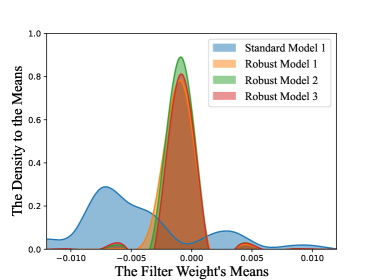
Figure 1: The distribution versus the means of filters’ weights in the second convolution layer in ResNet-18 on CIFAR-10 toward a standard model and three state-of-the-art robust models trained by [45, 61, 60]. The figure shows filters’ weight distribution exists an obvious difference for the standard and robust models.

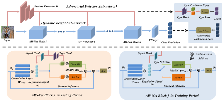
Figure 2: The framework of our AW-Net. AW-Net includes two main branches: the dynamic weight sub-network composed of multiple AW-Net blocks and the adversarial detector sub-network to discriminate the clean and adversarial example and generate the regulation signals. In the training period, we utilize the MixBN (including Adv BN and Clean BN) to handle different feature distributions of clean and adversarial examples, respectively. In the testing period, Adv BN and Clean BN are weighted by the prediction of adversarial detector.

To balance the trade-off between the accuracy and robustness, various methods are presented from different views, such as advanced optimization algorithm [57, 60] or modified network architecture [59, 30, 8], and so on. As for the former one, TRADES [57] attempts to reduce the gap by utilizing a Kullback–Leibler (KL) divergence loss in adversarial training. MTARD [60] applies two teacher models to guide a student model to promote the accuracy and robustness by adversarial distillation. As for the latter one, MagNet [30] tries to learn the clean distribution and then distinguish adversarial examples to be not recognized. However, it is not robust to the adaptive attack proposed by [3]. AdvProp [54] uses an auxiliary Batch-Normalization (BN) layer to improve the robustness and can achieve good accuracy on clean examples. Furthermore, Liu et al. [28] propose multiple BN layers to control the domain-specific statistics for different attack methods. Although they show some positive effects, the trade-off still exists and needs to be further studied.

To solve this problem, in this paper, we investigate the standard and robust models from the view of networks’ weight distribution. In Figure 1, we observe that filters’ weight distribution for the same network architecture between standard-trained and robust-trained models exist an obvious distinction, while the robust-trained models have the similar distribution. We analyse the underlying reason, and give a theoretical explanation for this phenomenon in terms of the gradient regularization of different optimization algorithms. The empirical and theoretical analysis indicate that a static network is challenging to eliminate the gap and is hard to improve both the accuracy and robustness because it is difficult to contain two groups of different weights within a static network. A reasonable solution is to adaptively change the network’s weights based on the input samples, and thus utilize the optimal weights to process them, respectively.

Inspired by the dynamic networks [14, 44, 26], we design the Adversarial Weight-Varied Network (AW-Net) to perform a “divide and rule” weight strategy for the clean and adversarial example. Specifically, AW-Net contains two branches: a dynamic weight sub-network and an adversarial detector sub-network. The dynamic weight sub-network is in charge of changing the network’s weights at the level of filters to process the clean and adversarial example, respectively. To handle different characteristic distributions of input samples and keep the model stable during training and testing, a MixBN [6, 28] structure is adapted into the sub-network. The adversarial detector sub-network is responsible for classifying the clean and adversarial example, and then produce the regulation signals to guide the weights’ change in the dynamic weight sub-network. These two sub-networks are jointly trained in an end-to-end adversarial training manner, and can interact with each other closely. With these careful designs, AW-Net has the potentiality to enhance the accuracy and robustness at the same. The flowchart is shown in Figure 2.

We summarize our contributions as follows:

• We empirically explore the difference existed between the standard-trained and robust-trained models versus the filters’ weight distribution for the same network architecture, and theoretically explain this phenomenon in terms of the gradient regularization. We argue that this difference may be one reason for the poor trade-off between the accuracy and robustness because it is hard to contain two groups of different weights in a static network.

• We propose a sample-wise dynamic network named Adversarial Weight-Varied Network (AW-Net), which dynamically adjusts the weights based on the input samples. For that, a dynamic weight sub-network at the filter level is designed, and a MixBN structure is used to handle the feature distributions for clean and adversarial examples. Meanwhile, we apply a multi-head adversarial detector sub-network to generate the regulation signal to guide the dynamic weights. Moreover, a joint training strategy is used to train AW-Net.

• We extensively verify the effectiveness of AW-Net on two public datasets, and compare with state-of-the-art robust models against the white-box and black-box attack, respectively. The results show that our method achieve the best performance versus the trade-off between the accuracy and robustness.

The rest of the paper is organized as follows: we introduce the related work in Section 2. Section 3 explores the differences for the filters’ weight distribution. We present the AW-Net in Section 4. The experiments are conducted in Section 5, and the conclusion is given in Section 6.

2 Related Work

2.1 Adversarial Attacks

Szegedy et al.[37] demonstrate that imperceptible adversarial perturbations on inputs can mislead the prediction of DNNs. After that, lots of adversarial attack methods are proposed, such as Fast Gradient Sign Method (FGSM)[10], Projected Gradient Descent Attack (PGD) [29], Carilini and Wagner Attack (C$\&$W) [4], and Jacobian-based Saliency Map Attack (JSMA) [32]. Generally speaking, adversarial attacks can be divided into white-box attacks [10, 29, 4] and black-box attacks [47, 27, 49, 48, 50, 46, 52]. White-box attacks usually generate adversarial examples based on the gradients of the target models. While black-box attacks perform attacks via the transfer-based strategy or query-based strategy according to how much information of the target model can be obtained.

In this paper, we propose a novel network architecture, and then test its robustness against the white-box and black-box attacks, respectively.

2.2 Adversarial Robustness

To defend against adversarial attacks, lots of researches are proposed to enhance the robustness. Adversarial Training [29, 45, 21, 22] is a representative method among them. Madry et al. [29] formulate Adversarial Training as a min-max optimization. Further, Adversarial Robustness Distillation (ARD) methods [9, 60] use strong teacher models to guide the adversarial training process of small student models to enhance the robustness. Meanwhile, many pre-processing methods are applied to remove the effects of adversarial perturbations. For example, [12, 2] utilize the encoder structure to denoise the adversarial examples, which shows competitive performance against adversarial attacks. Image compression operations are also verified to be effective to deal with adversarial perturbations, such as JPEG compression [5] and DCT compression [1], etc. In addition, re-normalizing the image from adversarial version to clean version [33, 8] can enhance the model robustness from the view of distribution. Shu et al.[33] use a batch normalization layer to achieve the clean feature by re-normalizing the adversarial feature with means and variances of clean features in adversarial training. Dong et al.[8] try to transform the adversarial feature into the clean distribution in object detection task.

We can see that all the above methods aim to improve the robustness for a static network. In contrast, our method designs a dynamic network to adaptively adjust the weights to process the input sample.

2.3 Trade-off between Accuracy and Robustness

The trade-off between accuracy and robustness has been widely studied [57, 58, 42, 55, 31, 60]. Zhang et al. [57] apply the prediction of clean examples to guide the training process toward adversarial examples (TRADES). Zhang et al. [58] enhance both accuracy and robustness by reweighting the training example. Stutz et al. [36] claim that manifold analysis can be helpful to achieve both accuracy and robustness. Yang et al. [55] argue that the trade-off can be mitigated by optimizing the locally lipschitz functions. Pang et al. [31] apply local equivariance to describe the ideal behavior of a robust model and facilitate the reconciliation between accuracy and robustness. Zhao et al. [60] apply multiple teacher models to improve the both accuracy and robustness of the student model.

In this paper, we attempt to understand accuracy and robustness directly from the perspective of model weight distributions and try to mitigate the trade-off between model accuracy and robustness with the architecture of dynamic network weights.

2.4 Dynamic Networks

Different from static networks, dynamic networks usually change their architectures based on the input samples [14, 40, 43]. The purpose of designing dynamic networks is to reduce the cost of network inference and utilize the most effective sub-networks to get the correct prediction. For example, Wang et al.[44] consider the filters as experts and select a part of them to activate some specific layers. Li et al.[26] propose the Dynamic Slimmable Network to divide the inputs into easy and hard samples and then design a dynamic network to predict samples’ type. Veit et al.[40] and Wang et al.[43] design to dynamically skip the residual structure and reduce the calculation cost.

Recently, the adversarial robustness of dynamic networks is evaluated [15, 18, 19]. [15] is the first work to show the vulnerability of dynamic networks. Hu et al.[19] argue that triple wins can be obtain for the accuracy, robustness, and efficiency via a multi-exit dynamic network. However, Hong et al. [18] show that the efficiency of this multi-exit network can be reduced by the proposed slowdown attack. Some methods named transductive defenses [41, 53] update the network’s parameters in the evaluation process to dynamically defend against adversarial examples.

We are different from the above works as follows: (1) we aim at defense rather than attacks like [15, 18]. (2) we focus on dynamically adjusting the network’s weights rather than utilizing the multi-exit layers like [19]. The motivation of our method is based on the filter’s weight observation in Figure 1, which has different defense mechanism with [19]. (3) During the testing phase, our method does not need to update the parameters, which is obviously different from transductive defenses [41, 53].

3 Filter Weight Distributions

3.1 Empirical Observation

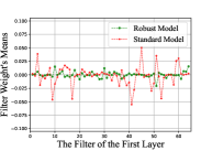
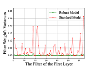
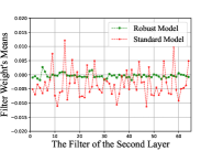
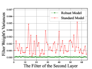
Figure 3: The visualization of filters’ means and variances for a strong standard model and a strong robust model trained by MART [45] on CIFAR-10. The left two figures are visualization of means and variances for the first layer in ResNet18; And the right two figures are visualization of means and variances for the second layer in ResNet 18. For simplicity, we only show these two layers, and the other layers also show the same phenomenon.

As mentioned before, although some models have shown the good adversarial robustness, their clean accuracy is always inferior to the standard models. To investigate the underlying reason, we pay attention to the network’s weights. Because filters can be approximately considered as the independent units of feature extracting, so we compute the means and variances of the filters at different convolution layers, and then use them to evaluate the weight distributions. Figure 1 shows that the means’ distribution between the standard and robust models varies greatly. To further explore this phenomenon, we directly illustrate the means and variances of a strong standard model and a strong robust model trained by [45] with the same network architecture in Figure 3.

From the results, we can see that the filter’s weight of the standard model shows a rough change, while the filter’s weight of the robust model shows a smooth change. This contrast illustrates the obvious difference between the standard and robust model. The prominent means and variances of the standard model demonstrate that it is easy to capture more subtle image features, which can explain why the standard model is easily affected by adversarial samples with minor perturbations. As a comparison, the robust model shows smaller means and variances and is more robust to the adversarial perturbations. Different weight sizes between standard and robust models may directly lead to the sensitivity to clean and adversarial examples and can further influence the model’s robustness.

3.2 Theoretical Analysis

Inspired by [34], we theoretically analyze the above performance from the perspective of model’s optimization, which directly influences the weight distribution. We investigate the intrinsic mechanisms of robust models using adversarial training methods based on PDG-AT [29] and TRADES [57] following [34]. Firstly, we analyze the optimization loss of standard models and adversarial models during the training process. The optimization loss $L_{adv}(x,y)$ for adversarial training and the optimization loss $L(x,y)$ for standard model training can be defined as follows:

$$L_{adv}(x,y)=\frac{1}{2}(L(x,y)+L(x+\delta,y)),$$ (1)

where $\delta$ represents the adversarial perturbation with the maximum perturbation scale $\epsilon$, and $x$ and $y$ refer to the input samples and true labels, respectively. By performing a first-order Taylor expansion on the loss $L_{adv}(x,y)$ for adversarial training, we can obtain:

$$L_{adv}(x,y) \approx\frac{1}{2}(L(x,y)+L(x,y)+\delta\cdot\partial_{x}L(x,y)),$$

$$=L(x,y)+\frac{1}{2}\delta\cdot\partial_{x}L(x,y),$$ (2)

where $\cdot$ denotes the matrix point multiplication operation, $\partial_{x}L(x,y)$ represents the first-order partial derivative of $L(x,y)$ with respect to $x$. Following [34], further expansion of $\partial_{x}L(x,y)$ can be obtained as follows:

$$\delta\cdot\partial_{x}L(x,y) =\mathop{\max}_{\mid\mid\delta\mid\mid_{p}\leq\epsilon}\mid L(x+\delta,y)-L(x,y)\mid,$$

$$\approx\mathop{\max}_{\mid\mid\delta\mid\mid_{p}\leq\epsilon}\mid\delta\cdot\partial_{x}L(x,y)\mid,$$

$$=\epsilon\mid\mid\partial_{x}L(x,y)\mid\mid_{q},$$ (3)

where $p$ denotes the $l_{p}$ norm, $\mid\mid.\mid\mid_{q}$ is the dual norm of $\mid\mid.\mid\mid_{p}$ and can be defined as follows:

$${\mid\mid z\mid\mid}_{q}=sup\left\{z^{T}x\ {\mid\mid x\mid\mid}_{p}\leq 1\right\}.$$ (4)

The regular term $\mid\mid\partial_{x}L(x,y)\mid\mid_{q}$ represents the result of regularization on the partial derivative of the optimization loss $L(x,y)$ with respect to the input data $x$. Furthermore, by substituting the derivation result back into Eq. (3.2), we can obtain the $L_{adv}(x,y)$ for adversarial training as follows:

$$L_{adv}(x,y)=L(x,y)+\frac{\epsilon}{2}{||\partial_{x}L(x,y)||}_{q}.$$ (5)

Based on the above results, the difference between the two training methods is that the optimization loss $L_{adv}(x,y)$ of the adversarial training adds a gradient regularization constraint based on the optimization loss $L(x,y)$ of the standard training, and the gradient regularization term constraint will directly affect the update of the model weight. Specifically, in the standard training process, the model weight $w_{nat}$ is updated based on the $L(x,y)$ according to the gradient descent criterion:

$$w_{nat}=w_{nat}-\eta\partial_{w_{nat}}L(x,y),$$ (6)

where $\eta$ is the learning rate of the weight, $\partial_{w_{nat}}L(x,y)$ is the partial derivative of the $L(x,y)$ relative to the weights $w_{nat}$. During the adversarial training process, the weights $w_{adv}$ are updated as follows:

$$w_{adv}=w_{adv}-\eta\partial_{w_{adv}}L_{adv}(x,y).$$ (7)

In the initial state, the model weight $w_{0}$ is randomly initialized with the same means and variances. Based on this assumption, whether a model obtained by standard training or a model obtained by adversarial training, the model weight $w_{0}$ in the initial state has the same distribution. Since the update of the model weight $w_{0}$ depends on the gradient descent criterion, after the loss function guide the update, the expectations of the model weight are respectively as follows:

$$E(w_{nat})=E(w_{0})-\eta E(\partial_{w_{0}}L(x,y)),$$ (8)

$$E(w_{adv})=E(w_{0})-\eta E(\partial_{w_{0}}L_{adv}(x,y)).$$ (9)

Then the weight distribution difference between the standard training model and the adversarial training model can be derived as follows:

$$E(\Delta_{w}) =\eta\mid\mid E(w_{adv})-E(w_{nat})\mid\mid,$$

$$=\eta\mid\mid E(\partial_{w_{0}}L_{adv}(x,y)-\partial_{w_{0}}L(x,y))\mid\mid,$$

$$=-\frac{\epsilon\eta}{2}E(\partial_{w_{0}}\mid\mid\partial_{x}L(x,y)\mid\mid_{q}).$$ (10)

The regular term ${\mid\mid\partial_{x}L(x,y)\mid\mid}_{q}$ can be used to measure the sensitivity of the input sample $x$ in the model distribution space: when the value of ${\mid\mid\partial_{x}L(x,y)\mid\mid}_{q}$ is large, small perturbation in $x$ will lead to obvious fluctuation in the prediction results of the model; When the value of ${\mid\mid\partial_{x}L(x,y)\mid\mid}_{q}$ is small, the prediction results of the model are not sensitive to small perturbation in $x$. After using it as the loss function for training optimization toward model weight $w_{0}$ , the partial derivative $\partial_{w_{0}}{\mid\mid\partial_{x}L(x,y)\mid\mid}_{q}$ of the model weight with respect to the regular term can optimize the sensitivity of the model weight toward $x$. In other words, after the constraints of the model weight, the final prediction does not change significantly when $x$ is perturbed within perturbation scale $\epsilon$.

Therefore, the optimization process of the adversarial training model is constrained by the regularization term ${\mid\mid\partial_{x}L(x,y)\mid\mid}_{q}$, the model is not obvious for the adversarial perturbation $\delta$ of the input $x$, which may be the inherent mechanism of strong robustness to adversarial examples; In contrast, the optimization of standard training is limited to the loss $L(x,y)$, after gradient descent operation, the model weight $w$ is only affected by the clean examples, and can achieve a pretty performance. Since the optimization process is not constrained by the regularization term ${\mid\mid\partial_{x}L(x,y)\mid\mid}_{q}$, the standard training does not take into account the change of the model prediction results when $x$ is slightly perturbed, which leads to weak robustness. Due to the term of gradient regularization, adversarial training and standard training will lead to different sensitivity for model weight to different types of samples, which directly leads to a significant gap between the robust model and the standard model.

Based on the above observation and the theoretical analysis, we argue it is difficult to contain two groups of weights with different distributions in a static network. Inspired by dynamic networks, we consider to replace static networks with dynamic networks. A sample-wise dynamic network model can change the model weight according to the input samples, which provides the potentiality to solve the trade-off between the accuracy and robustness.

4 Adversarial Weight-Varied Network

4.1 Overview

The pipeline of the proposed framework is shown in Figure 2. We propose a sample-wise dynamic Adversarial Weight-Varied Network (AW-Net) to enhance the accuracy and robustness. AW-Net contains two branchs: a dynamic weight sub-network and an adversarial detector sub-network. The dynamic weight sub-network applies different filters’ weights to adapt various inputs. Meanwhile, MixBN is used to handle the different distribution of clean and adversarial examples, respectively. The adversarial detector sub-network is used to generate regulation signals to adjust the filters’ weights of dynamic weight sub-network.

4.2 Dynamic Weight Sub-network

The analysis in Section 3 inspires us to design a dynamic network composed of multiple AW-Net blocks which can dynamically adjust the filter weights. For the $j$-th block, we assume $\psi_{j}\in\mathbb{R}^{c^{in}_{j}\times w_{j}^{in}\times h_{j}^{in}}$ is the input feature with $c^{in}_{j}$ channels, and $\phi_{j}\in\mathbb{R}^{c^{out}_{j}\times w_{j}^{out}\times h_{j}^{out}}$ is the output feature with $c^{out}_{j}$ channels. We utilize a residual structure to construct each block in AW-Net. Specifically, the $j$-th block is defined as follows:

$$\phi_{j}=\sigma(\mathcal{F}_{j}(\psi_{j})+\psi_{j}),$$ (11)

where $\sigma(\cdot)$ denotes the Relu layer. The symbol $\mathcal{F}_{j}(\cdot)$ contains the convolution layer $\mathcal{W}^{conv}_{j}\in\mathbb{R}^{c^{in}_{j}\times k_{j}\times k_{j}\times c^{out}_{j}}$ with kernel size $k_{j}$ and other nonlinear layers such as Batch-Normalization layer. $\mathcal{W}^{conv}_{j}$ consists of multiple filters $\mathcal{K}_{m}\in\mathbb{R}^{c^{in}_{j}\times k_{j}\times k_{j}},m=(1,2,...,c^{out}_{j})$, thus:

$$\mathcal{W}^{conv}_{j}=concat(\mathcal{K}_{1},...,\mathcal{K}_{c_{out}}),$$ (12)

where $concat(\cdot)$ is the concatenate operation along with the forth dimension. Without losing generality, different filters in convolution layer $\mathcal{W}^{conv}_{j}$ can be viewed as relatively independent units for extracting feature information and are similar to the individual “experts”. From this point of view, different filters $\mathcal{K}_{m}$ in our AW-Net block are supposed to have different importance when processing adversarial and clean samples. In order to make each filter play its speciality, we apply a filter-wise vector $\omega_{j}=(\omega^{1}_{j},...,\omega^{c_{out}}_{j})$ to give them different regulation signals as follows:

$$\mathcal{\hat{W}}^{conv}_{j}=concat(\omega^{1}_{j}\cdot\mathcal{K}_{1},...,\omega^{c_{out}}_{j}\cdot\mathcal{K}_{c_{out}}),$$ (13)

then we perform a convolution operation $*$ to obtain the output feature:

$$\pi_{j}=\mathcal{\hat{W}}^{conv}_{j}*\psi_{j}.$$ (14)

With the assistance of weight adjustment, the block can deal with adversarial and clean example in a distinctive way of feature processing. For the adversarial example, the filters’ weights will have small variances and filters’ weights will have large variances for clean examples, as the phenomenon shown in Figure 3.

Batch Normalization [20] is an effective method to accelerate the training process, and is usually attached after the convolution layer. However, the existence of BN layer will eliminate the feature difference between adversarial and clean examples, and make their distributions tend to be the same. The weight adjustment mechanism toward filters will not take advantage of handling different characteristics and may negatively influence the performance of the network, leading to the catastrophic results that both distributions cannot be fitted well.

Inspired by the gated batch normalization [28] , we design a MixBN, where a Clean BN $BN_{nat}$ is used to handle the features $\pi_{j}^{nat}$ of clean examples $x_{nat}$ and Adv BN $BN_{adv}$ is used to handle the features $\pi_{j}^{adv}$ of adversarial examples $x_{adv}$.

In the training process of the MixBN structure, the category of features can be obtained and we perform an operation of type selection, and separately train the Adv BN and Clean BN with adversarial examples $x_{adv}$ and clean examples $x_{nat}$. The training process of MixBN can be denoted as follows:

$$\begin{split}BN_{mix}=\left\{\begin{array}[]{ll}BN_{adv}(\pi_{j}^{adv}),&\psi^{adv}_{j}\propto x_{adv},\\ BN_{nat}(\pi_{j}^{nat}),&\pi_{j}^{nat}\propto x_{nat}.\end{array}\right.\end{split}$$ (15)

In the testing process of the MixBN structure, we use type predictions $P_{type}$ (defined in the next section) from the adversarial detector sub-network as different BN’s weights and use both Adv BN and Clean BN to deal with input features. The test process of MixBN can be denoted as follows:

$$\begin{split}BN_{mix}=(1-P_{type})&BN_{adv}(\pi_{j}^{adv})\\ &+P_{type}BN_{nat}(\pi_{j}^{nat}).\end{split}$$ (16)

After the above operations, $\mathcal{F}_{j}(\cdot)$ is defined as:

$$\mathcal{F}_{j}(\psi_{j})=BN_{mix}(\mathcal{\hat{W}}^{conv}_{j}*\psi_{j}).$$ (17)

Here, we use a two-layer residual structure, thus the $j$-th block is finally formulated as follows:

$$\phi_{j}=\sigma(\mathcal{F}_{j}(\sigma(\mathcal{F}_{j}(\psi_{j})))+\psi_{j}).$$ (18)

The prerequisite for an effective dynamic weight sub-network is based on the excellent performance of regulation signals $\omega_{j}$ and type predictions $P_{type}$ in the testing process. So how to design an effective adversarial detector sub-network is needed to be solved.

4.3 Adversarial Detector Sub-network

We design a lightweight sample-wise adversarial detector sub-network, including a feature extractor and an adversarial weight regulator structure. The feature extractor is designed for getting semantic features from inputs and the following adversarial regulator structure is used to analyse the semantic features and generate guiding information toward dynamic weight sub-network.

Here a backbone network is used as the feature extractor $\mathcal{D}$ to get the representative feature from origin images $x$. To facilitate subsequent processing for weight regulator, we get an one-dimension feature map $\psi_{M}\in\mathbb{R}^{d}$ after feature extractor $\mathcal{D}$. The operation can be denoted as follows:

$$\psi_{M}=\mathcal{D}(x).$$ (19)

Then the feature map $\psi_{M}$ is processed by the adversarial weight regulator, which has a type head to get the type predictions $P_{type}$ of input samples and signal heads to generate regulation signals $\omega_{j}$.

For the design of type head structure, we use a fully connected layer $\mathcal{W}^{type}\in\mathbb{R}^{2\times d}$, and a softmax operation is applied to get the type predictions $P_{type}$. The type head structure can be formulated as follows:

$$P_{type}=softmax(\mathcal{W}^{type}\psi_{M}).$$ (20)

For the design of signal head structure, in order to make full use of the entire information, individual signal heads are applied to generate regulation signals $\omega_{j}$ for each $j$-th block. Thus it is called as multi-head adversarial detetor sub-network. It can adjust the filter weights following Eq.(14) and allow every blocks to extract different semantic information of adversarial and clean examples at the filter level. Due to the instability of the neural network, directly using the feature map as regulation signals may lead to huge fluctuations whether in the training or testing process. Hence, a normalization operation toward the signal head are supposed to reduce the volatility. Here we use the $tanh$ based function to make regulation signals more stable and can be formulated as follows:

$$\omega_{j}=\big{[}tanh(\mathcal{W}_{j}\psi_{M})+1\big{]}^{\beta},$$ (21)

where $\mathcal{W}_{j}\in\mathbb{R}^{c_{out}\times d}$ denotes the fully connected layer for the $j$-th block. $\beta$ is a trade-off parameter to control the strength for guidance, if $\beta$ is too high, the effect of weight adjustment will be too strong, and the network inference will be unstable. If $\beta$ is too low, it will be difficult to distinguish adversarial and clean examples.

All in all, with the favorable support of the adversarial detector sub-network, the dynamic weight sub-network can give full play to its ability to deal with adversarial and clean examples with different weights.

4.4 Joint Adversarial Training

Similar to the static networks, our AW-Net can also be trained using the existing various adversarial training algorithms based on the min-max formulation [29], such as TRADES [57], MART [45], and so on. However, to make full use of the dynamic characteristic in AW-Net, we choose Multi-teacher adversarial distillation (MTARD) [60] as the adversarial training algorithm to perform a joint training strategy. MTARD utilizes a clean teacher and a robust teacher to jointly train the network to achieve the balance between accuracy and robustness, which is highly compatible to our AW-Net. Specifically, we can apply these two teachers to train the different weights for the clean examples and adversarial examples, respectively. Clean examples are trained by the strong standard teacher $T_{nat}$, and adversarial examples are trained by a strong adversarial teacher $T_{adv}$, which is formulated as follow:

$$\mathcal{L}_{adv}=\tau^{2}\mathcal{L}_{KL}(S^{\tau}(x_{adv}),T_{adv}^{\tau}(x_{adv})),$$ (22)

$$\mathcal{L}_{nat}=\tau^{2}\mathcal{L}_{KL}(S^{\tau}(x_{nat}),T_{nat}^{\tau}(x_{nat})),$$ (23)

where $\mathcal{L}_{nat}$ and $\mathcal{L}_{adv}$ denote adversarial distillation loss for clean and adversarial teacher, respectively, $\mathcal{L}_{KL}$ denotes the Kullback-Leibler Divergence loss, $S(\cdot)$ denotes AW-Net, and $S^{\tau}(\cdot)$ denotes the tempered variant of $S(\cdot)$ with temperature $\tau$ [17]. Also, we design a classification loss to train the adversarial detector sub-network to get type predictions. The minimization loss of training the AW-Net is as follows:

$$\mathcal{L}_{total}=\mathcal{L}_{type}(P_{type},y^{\prime})+\alpha_{1}\mathcal{L}_{adv}+\alpha_{2}\mathcal{L}_{nat},$$ (24)

where $\mathcal{L}_{type}$ denotes the type loss for the binary classification, $y^{\prime}$ is a label that can represent adversarial and clean types. $\alpha_{1}$ and $\alpha_{2}$ are the hy-parameters, which will be automatically adjusted in the training process as described in their original paper [60]. Therefore, we don’t manually tune them in the experiment.

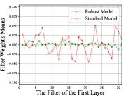
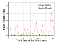
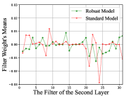
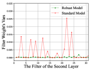
Figure 4: The visualization of filters’ means and variances for a strong standard model and a strong robust model trained by MTARD [60] on CIFAR-10. The left two figures are visualization of means and variances for the first layer in MobileNet-v2; And the right two figures are visualization of means and variances for the second layer in MobileNet-v2.

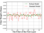
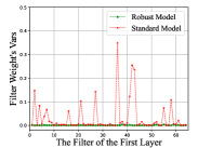
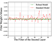
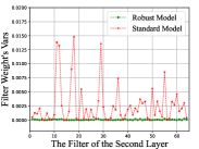
Figure 5: The visualization of filters’ means and variances for a strong standard model and a strong robust model trained by MTARD [60] on CIFAR-10. The left two figures are visualization of means and variances for the first layer in ResNet-50; And the right two figures are visualization of means and variances for the second layer in ResNet-50.

4.5 More details about AW-Net

For the dynamic weight sub-network, we replace the whole two-layer basic block with our AW-Net block mentioned in Section 4.2 based on the ResNet-18 [16], and the dimension of the final fully-connected layer adapts to the $x$’s dimension of different applied dataset (e.g. CIFAR and Tiny-ImageNet) by average pooling operation.

For the adversarial detector sub-network, an one-dimensional vector $\psi_{M}$ of 512 size is obtained after the process of a lightweight feature extractor $\mathcal{D}$. Then the feature vector $\psi_{M}$ is processed by the type head and the signal head mentioned in Section 4.3. After the process of type head $\mathcal{W}^{type}$, the feature vector $\psi_{M}$ transform into a 2-dimensional vector to predict the type predictions $P_{type}$. For the signal head $\mathcal{W}_{j}$ in $j$-th block, due to the two-layer block design in our setting, two individual signal heads $\mathcal{W}_{j}$ are applied for two convolution layers in a block $\mathcal{W}^{conv}_{j}$ respectively and other setting is following the origin setting.

5 Experiment

5.1 Experiment Settings

Datasets: We conduct the experiments on two public datasets, including CIFAR-10 [23], CIFAR-100 and Tiny-ImageNet [24]. For CIFAR-10 and CIFAR-100, the image size is 32 $\times$ 32, training set contains 50,000 images, and testing set contains 10,000 images. CIFAR-10 covers 10 classes while CIFAR-100 covers 100 classes. For Tiny-ImageNet dataset, the image size is 64 $\times$ 64. The training set contains 100,000 images, and testing set contains 10,000 images, covering 200 classes.

Compared SOTA methods: Because our method proposes a novel network architecture, we compare with other state-of-the-art network architectures with similar parameter scales. To ensure fair comparisons, all the networks are trained with the same optimization algorithm. Specifically, for CIFAR-10 and CIFAR-100, the compared networks include ResNet-34 [16], ResNet-50 [16], WideResNet-34-8 [56], VGG-16-BN [35] and RepVGG-A2 [7]. All of them are trained by the same state-of-the-art adversarial distillation method [60] with multi-teachers. In addition, we also compare with a robust dynamic network [19].

Evaluation metric: Here we use the Weighted Robust Accuracy (W-Robust Acc) following [13] to comprehensively evaluate the accuracy and robustness, which is as follows:

$$\mathcal{A}_{w}=\gamma_{nat}\mathcal{A}_{nat}+\gamma_{adv}\mathcal{A}_{adv},$$ (25)

where $\mathcal{A}_{w}$ is the W-Roubst Acc computed from the clean accuracy $\mathcal{A}_{nat}$ and the adversarial accuracy $\mathcal{A}_{adv}$. We set $\gamma_{nat}$ and $\gamma_{adv}$ both to 0.5.

Implementation details: On CIFAR-10 and CIFAR-100 datasets, we use ResNet-18 as the basis to construct the dynamic weight sub-network, and then modify each residual block according to Section 4.2. Note that users can also adapt other networks like ResNet-34 and ResNet-50. The training optimizer is Stochastic Gradient Descent (SGD) optimizer with momentum 0.9 and weight decay 2e-4, and the initial learning rate is 0.1 for the dynamic weight network and 0.01 for the adversarial weight regulator, and the gradient of the feature extractor does not be updated.

We train all the above models for 300 epochs, and the learning rate is divided by ten at the 215-th, 260-th, and 285-th epoch, and the batch size is 128. We use PGD-10 (10 step PGD) to generate adversarial examples $x_{adv}$ with random start size 0.001 and step size 2/255, and the perturbation is bounded to the $L_{\infty}$ norm $\epsilon$ = 8/255. $\beta$ is set to 4 for CIFAR-10 and 1 for CIFAR-100, respectively. And $\tau$ is set to 1 for CIFAR-10 and 5 for CIFAR-100. The teacher models on CIFAR-10 and CIFAR-100 follow the setting in [60].

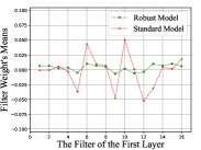
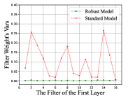
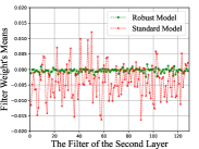
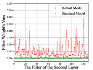
Figure 6: The visualization of filters’ means and variances for a strong standard model and a strong robust model trained by MTARD [60] on CIFAR-10. The left two figures are visualization of means and variances for the first layer in WideResNet-34-8; And the right two figures are visualization of means and variances for the second layer in WideResNet-34-8.

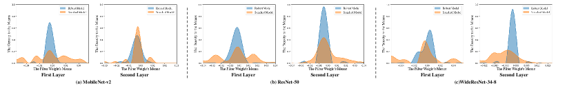
Figure 7: The distribution versus the means of filters’ weights in the first and second convolution layer in MobileNet-v2, ResNet-50, and WideResNet-34-8 on CIFAR-10 toward standard models and robust models trained by [60].

5.2 More Results about Filter Weight Distribution

In order to better validate the weight difference between the robust model and the standard model, we validate against different network architectures. Here, in addition to the ResNet-18 network structures selected in Figure 3, we also chose three different network structures: including MobileNet-v2, ResNet-50, and WideResNet-34-8. The robust models are trained by MTARD [60]. The results are shown in Figure 4, Figure 5, and Figure 6. Also, we visualize the weight distribution for the above three models and the result is shown in Figure 7.

The results show that the phenomenon about weight gap widely exists in different network structures but not just limited a particular network structure, which can effectively support our empirical judgment and theoretical analysis on the model weights’ gap between the clean model and the robust model.

TABLE I: White-box robustness on CIFAR-10 and CIFAR-100 datasets. All the models are trained following the state-of-the-art adversarial training method MTARD [60]. All the results are the best checkpoints based on W-Robust Acc.

			CIFAR-10			CIFAR-100
Attack	Model	Params (M)	$\mathcal{A}_{nat}$	$\mathcal{A}_{adv}$	$\mathcal{A}_{w}$	$\mathcal{A}_{nat}$	$\mathcal{A}_{adv}$	$\mathcal{A}_{w}$
FGSM	ResNet-34[16]	20.33 M	90.30%	58.18%	74.24%	65.69%	33.47%	49.58%
	ResNet-50[16]	22.63 M	90.22%	60.65%	75.44%	69.59%	33.68%	51.64%
	WideResNet-34-8[56]	29.51 M	90.14%	62.23%	76.19%	60.46%	25.67%	43.07%
	VGG-16-BN[35]	32.21 M	86.89%	57.49%	72.19%	57.65%	28.23%	42.94%
	RepVGG-A2[7]	25.64 M	81.05%	47.35%	64.20%	51.44%	24.23%	37.84%
	AW-Net (ours)	26.32 M	91.49%	79.14%	85.32%	72.85%	49.19%	61.02%
PGDsat	ResNet-34[16]	20.33 M	90.30%	45.56%	67.93%	65.69%	25.85%	45.77%
	ResNet-50[16]	22.63 M	90.22%	47.26%	68.74%	69.59%	25.02%	47.31%
	WideResNet-34-8[56]	29.51 M	90.14%	50.74%	70.44%	60.46%	20.05%	40.26%
	VGG-16-BN[35]	32.21 M	86.89%	44.53%	65.71%	57.65%	20.88%	39.27%
	RepVGG-A2[7]	25.64 M	81.05%	35.17%	58.11%	51.44%	17.90%	34.67%
	AW-Net (ours)	26.32 M	91.49%	50.51%	71.00%	72.85%	24.83%	48.84%
PGDtrades	ResNet-34[16]	20.33 M	90.30%	48.95%	69.63%	65.69%	27.77%	46.73%
	ResNet-50[16]	22.63 M	90.22%	51.27%	70.75%	69.59%	27.38%	48.49%
	WideResNet-34-8[56]	29.51 M	90.14%	53.69%	71.92%	60.46%	21.70%	41.08%
	VGG-16-BN[35]	32.21 M	86.89%	48.46%	67.68%	57.65%	22.83%	40.24%
	RepVGG-A2[7]	25.64 M	81.05%	38.67%	59.86%	51.44%	19.33%	35.39%
	AW-Net (ours)	26.32 M	91.49%	53.19%	72.34%	72.85%	24.66%	48.76%
CW∞	ResNet-34[16]	20.33 M	90.30%	45.95%	68.13%	65.69%	24.67%	45.18%
	ResNet-50[16]	22.63 M	90.22%	47.44%	68.83%	69.59%	25.36%	47.48%
	WideResNet-34-8[56]	29.51 M	90.14%	50.06%	70.10%	60.46%	18.84%	39.65%
	VGG-16-BN[35]	32.21 M	86.89%	44.22%	65.56%	57.65%	20.02%	38.84%
	RepVGG-A2[7]	25.64 M	81.05%	34.74%	57.90%	51.44%	16.79%	34.12%
	AW-Net (ours)	26.32 M	91.49%	47.65%	69.57%	72.85%	23.02%	47.94%

5.3 Robustness Evaluation

Robustness against White-box Attacks. We evaluate AW-Net and other comparison models against four white-box attack methods: FGSM [10], PGD_sat [29], PGD_trades [57], CW_∞ [4]. The step size of both two PGD attacks is 2/255 and total step is 20, the difference of two PGD attacks lies in the initialization. The step of CW_∞ is 30, and the perturbation of PGD and CW_∞ is bounded to the $L_{\infty}$ norm $\epsilon$ = 8/255.

Based on the results in Table I, we find AW-Net can achieve the best W-Robust Acc compared with state-of-the-art robust models with similar parameter scales. On CIFAR-100, AW-Net improves improves W-Robust Acc by 1.53% against PGD_sat attack compared with other robust models. The relevant advantages also display in the evaluation on other dataset (CIFAR-10) and other attack (FGSM, PGD_trades, and CW_∞).

TABLE II: Black-box robustness on CIFAR-10 and CIFAR-100 dataset. All the models are trained following the same state-of-the-art adversarial training method MTARD [60]. All the results are the best checkpoints based on W-Robust Acc.

			CIFAR-10			CIFAR-100
Attack	Model	Params (M)	$\mathcal{A}_{nat}$	$\mathcal{A}_{adv}$	$\mathcal{A}_{w}$	$\mathcal{A}_{nat}$	$\mathcal{A}_{adv}$	$\mathcal{A}_{w}$
PGDsat	ResNet-34[16]	20.33 M	90.30%	67.67%	78.99%	65.69%	41.92%	53.81%
	ResNet-50[16]	22.63 M	90.22%	68.31%	79.27%	69.59%	45.13%	57.36%
	WideResNet-34-8[56]	29.51 M	90.14%	68.40%	79.27%	60.46%	38.81%	49.64%
	VGG-16-BN[35]	32.21 M	86.89%	65.93%	76.41%	57.65%	38.85%	48.25%
	RepVGG-A2[7]	25.64 M	81.05%	62.62%	73.84%	51.44%	36.21%	43.83%
	AW-Net (ours)	26.32 M	91.49%	70.11%	80.80%	72.85%	42.76%	57.81%
CW∞	ResNet-34[16]	20.33 M	90.30%	67.30%	78.80%	65.69%	42.10%	53.90%
	ResNet-50[16]	22.63 M	90.22%	68.12%	79.17%	69.59%	44.93%	57.26%
	WideResNet-34-8[56]	29.51 M	90.14%	67.53%	78.84%	60.46%	39.37%	49.92%
	VGG-16-BN[35]	32.21 M	86.89%	65.39%	76.14%	57.65%	39.21%	48.43%
	RepVGG-A2[7]	25.64 M	81.05%	62.41%	71.73%	51.44%	37.08%	44.26%
	AW-Net (ours)	26.32 M	91.49%	69.94%	80.72%	72.85%	43.33%	58.09%

Robustness against Black-box Attacks. Similar to other works [45, 25, 57], we use the transfer-based attacks to evaluate the models’ black-box robustness. For that, we conduct the white-box attacks on a surrogate model, and then evaluate the black-box robustness using these generated adversarial examples. Here, we select the strong robust model: WideResNet-70-16 [11] as surrogate model to generate adversarial examples. The used black-box attacks are PGD_sat and CW_∞.

The results in Table II show that our AW-Net can outperform the state-of-the-art robust models and achieve better W-robust Acc. AW-Net improve W-robust Acc by 1.53% and 1.55% on CIFAR-10 against PGD_sat attack and CW_∞ attack respectively. Meanwhile, AW-Net can achieve similar performance on CIFAR-100, which has an improvement of 0.83% against the CW_∞ attack. The robustness against black-box attacks shows the effectiveness of our AW-Net.

5.4 Ablation Study

In order to verify the effectiveness of each component in our AW-Net, we conduct a set of ablation studies. Initially, we apply the adversarial detector sub-network to generate adversarial regulation signals and guide the dynamic weight network to distinguish clean and adversarial examples for different filters but without MixBN structure. Then, we explore the improvement brought by MixBN structure but without type predictions from the adversarial detector sub-network in the testing process, which only use the Adv BN. Furthermore, we use type predictions as MixBN weights, which is the final structure of our AW-Net. Meanwhile, to better show the effectiveness, we also report the performance of the baseline network: ResNet-18 as the comparison. The results are shown in Table III.

From the Table III, we see that only using the dynamic weight cannot achieve the good performance. After adding the MixBN, the performance achieve a remarkable increase, which shows the necessity to use MixBN to encode different feature distributions for clean and adversarial examples. Meanwhile, when the MixBN is weighted with the type predictions, the performance has also been obviously improved, showing the effectiveness of the adversarial detector sub-network. As a comparison with the Baseline network, our dynamic network achieves a nearly 2% improvement, showing the effectiveness of our idea.

TABLE III: Ablation study toward each component of AW-Net. “Dynamic Weight” denotes the dynamic weight sub-network with the guidance of the adversarial detector; “MixBN” represents using the MixBN layer instead of single BN layer in the dynamic weight sub-network; “Type Head” denotes using the type predictions in the adversarial detector sub-network as the weights of MixBN. “Baseline” is the basis network structure to construct AW-Net.

Attack	Dynamic Weight	MixBN	Type Head	$\mathcal{A}_{w}$
PGDtrades	✓	$\times$	$\times$	44.10%
	✓	✓	$\times$	67.31%
	✓	✓	✓	72.34%
		Baseline		70.48%
CW∞	✓	$\times$	$\times$	43.02%
	✓	✓	$\times$	66.67%
	✓	✓	✓	69.57%
		Baseline		67.97%

5.5 Different Training Methods

Here we try to explore the effect of different training algorithm on our AW-Net. We choose two different state-of-the-art methods, MTARD [60] and TRADES [57], and visualize the performance and the training loss of AW-Net on CIFAR-10 and CIFAR-100 in Figure 8. The results show the model trained based on MTARD has better performances than TRADES, our model can achieve good performance with the help of MTARD.

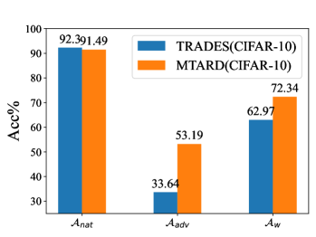
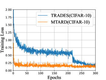
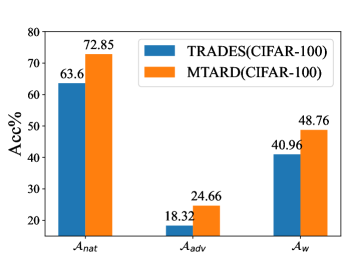
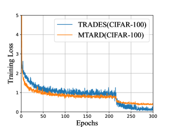
Figure 8: The performance and training loss of AW-Net trained by TRADES and MTARD on CIFAR-10 (Top) and CIFAR-100 (Bottom), respectively. All the results are the best checkpoints based on W-Robust Accuracy.

5.6 Experiment for $\beta$ in AW-Net

Here we explore the role of $\beta$ in 14 used in our AW-Net. We select the AW-Net trained on CIFAR-10 and test the results using different $\beta$ values. The results are shown in Table IV. The results show that the proper parameter settings has an influence on the final results. If $\beta$ is too high, the network will fluctuate and lead to a lower performance. If $\beta$ is too low, the adversarial and clean examples will be not recognized well. Finally, we choose the $\beta$ as 4 in our setting for CIFAR-10 and CIFAR-100.

TABLE IV: The performance of AW-Net with different $\beta$. All the results are the best checkpoints based on $\mathcal{A}_{w}$.

Attack	$\beta$ value	$\mathcal{A}_{nat}$	$\mathcal{A}_{adv}$	$\mathcal{A}_{w}$
PGDsat	$\beta=1$	90.30%	50.63%	70.47%
	$\beta=4$	91.49%	50.44%	71.00%
	$\beta=5$	92.04%	48.23%	70.14%
CW∞	$\beta=1$	90.30%	48.36%	69.33%
	$\beta=4$	91.49%	47.65%	69.57%
	$\beta=5$	92.04%	46.16%	69.10%

TABLE V: The White-box Robustness of AW-Net and [19].

Attack	model	$\mathcal{A}_{nat}$	$\mathcal{A}_{adv}$	$\mathcal{A}_{w}$
PGDsat	RDI-ResNet-38 [19]	83.79%	43.28%	63.54%
	AW-Net (ours)	91.49%	50.44%	71.00%

TABLE VI: White-box Robustness on Tiny-ImageNet. All the results are the best checkpoints based on $\mathcal{A}_{w}$.

Attack	models	$\mathcal{A}_{nat}$	$\mathcal{A}_{adv}$	$\mathcal{A}_{w}$
FGSM	ResNet-34	47.00%	41.30%	44.15%
	AW-Net(ours)	64.44%	32.83%	48.64%
PGDsat	ResNet-34	47.00%	22.70%	34.85%
	AW-Net(ours)	64.44%	15.61%	40.03%
PGDtrades	ResNet-34	47.00%	23.83%	35.42%
	AW-Net(ours)	64.44%	14.14%	39.29%
CW∞	ResNet-34	47.00%	20.94%	33.97%
	AW-Net(ours)	64.44%	13.43%	38.94%

TABLE VII: Adaptive Attack toward AW-Net. The robust accuracy is evaluated based on PGD_trades.

Dataset	Attacks	$\mathcal{A}_{adv}$
CIFAR-10	PGDtrades	50.51%
	Adaptive attack	50.22%
CIFAR-100	PGDtrades	24.83%
	Adaptive attack	26.21%

5.7 Other Dynamic Networks

Besides the static networks above, we here compare our AW-Net with a robust multi-exit dynamic weight network: RDI-ResNet-38 [19]. The evaluation is based on the PGD_sat with step 20. The result is shown in Table V, where shows that AW-Net has an obvious advantage compared with RDI-ResNet-38 [19]. The W-Robust Accuracy is improved from 63.54% to 71.00%, which demonstrates the effectiveness of the proposed dynamic network versus the varied-weights.

5.8 Robustness on Tiny-ImageNet

For Tiny-ImageNet dataset, we compare with the ResNet-34 [16]. Both our AW-Net and the baseline ResNet-34 are trained with state-of-the-art adversarial training algorithm: MTARD [60], the setting is also consistent. We train the above models for 50 epochs, and the learning rate is divided by 25-th and 40-th epoch, and the batch size is 64. $\beta$ is set to 1 and $\tau$ is set to 5.

The results on the Tiny-ImageNet are given in Table VI, showing that AW-Net can outperform ResNet-34 model when facing different attacks. Specifically, AW-Net improves W-Robust Acc by 4.49% against FGSM attack and improves W-Robust Acc by 5.18% against PGD_sat attack. The results show that AW-Net can achieve better performance with both accuracy and robustness, and is still effective in more challenging dataset.

5.9 Adaptive Attack

According to the adaptive attack definition in [39], we augment the original objective function used in the PGD_trades attack with our joint training loss (i.e., Eq.(14) in the original paper) to implement adaptive attacks. The comparison results of CIFAR-10 and CIFAR-100 under different attacks are shown in Table VII. Under the adaptive attack, we see that the Robust Accuracy of CIFAR-10 is 50.22%, which is almost the same with the W-Robust Accuracy under the original PGD_trades attack (50.51%). In CIFAR-100 dataset, the W-Robust Accuracy under adaptive attack is even slightly higher than that under the original attack (26.21% vs 24.83%). These results verify the robustness of AW-Net against adaptive attacks.

6 Conclusion

In this paper, we investigated the state-of-the-art method and explored the reason of the accuracy and robustness of the model cannot be achieved simultaneously from the empirical and theoretical perspective. We argued that it may be caused by the gap in the filters’ weight distribution. Based on the above observation, we proposed the Adversarial Weight-Varied Network (AW-Net) to deal with the clean and adversarial example with different filters’ weights to self-adapt input samples. We used MixBN to fit the distributions of clean and adversarial examples, and applied an adversarial detector sub-network to distinguish the clean and adversarial sample. The generated regulation signals were applied to guide the adjustment of the dynamic network. A series of solid experiments proved that AW-Net could achieve state-of-the-art performance in W-Robust accuracy compared with other robust models on three datasets.

References

- [1] Akhtar, N., Liu, J., Mian, A.: Defense against universal adversarial perturbations. In: Proceedings of the IEEE Conference on Computer Vision and Pattern Recognition. pp. 3389–3398 (2018)
- [2] Bai, W., Quan, C., Luo, Z.: Alleviating adversarial attacks via convolutional autoencoder. In: 2017 18th IEEE/ACIS International Conference on Software Engineering, Artificial Intelligence, Networking and Parallel/Distributed Computing (SNPD). pp. 53–58. IEEE (2017)
- [3] Carlini, N., Wagner, D.: Magnet and” efficient defenses against adversarial attacks” are not robust to adversarial examples. arXiv preprint arXiv:1711.08478 (2017)
- [4] Carlini, N., Wagner, D.: Towards evaluating the robustness of neural networks. In: 2017 ieee symposium on security and privacy (sp). pp. 39–57. IEEE (2017)
- [5] Das, N., Shanbhogue, M., Chen, S.T., Hohman, F., Chen, L., Kounavis, M.E., Chau, D.H.: Keeping the bad guys out: Protecting and vaccinating deep learning with jpeg compression. arXiv preprint arXiv:1705.02900 (2017)
- [6] Deecke, L., Murray, I., Bilen, H.: Mode normalization. arXiv preprint arXiv:1810.05466 (2018)
- [7] Ding, X., Zhang, X., Ma, N., Han, J., Ding, G., Sun, J.: Repvgg: Making vgg-style convnets great again. In: Proceedings of the IEEE/CVF Conference on Computer Vision and Pattern Recognition. pp. 13733–13742 (2021)
- [8] Dong, Z., Wei, P., Lin, L.: Adversarially-aware robust object detector. arXiv preprint arXiv:2207.06202 (2022)
- [9] Goldblum, M., Fowl, L., Feizi, S., Goldstein, T.: Adversarially robust distillation. In: Proceedings of the AAAI Conference on Artificial Intelligence. vol. 34, pp. 3996–4003 (2020)
- [10] Goodfellow, I.J., Shlens, J., Szegedy, C.: Explaining and harnessing adversarial examples. arXiv preprint arXiv:1412.6572 (2014)
- [11] Gowal, S., Qin, C., Uesato, J., Mann, T., Kohli, P.: Uncovering the limits of adversarial training against norm-bounded adversarial examples. arXiv preprint arXiv:2010.03593 (2020)
- [12] Gu, S., Rigazio, L.: Towards deep neural network architectures robust to adversarial examples. arXiv preprint arXiv:1412.5068 (2014)
- [13] Gürel, N.M., Qi, X., Rimanic, L., Zhang, C., Li, B.: Knowledge enhanced machine learning pipeline against diverse adversarial attacks. In: International Conference on Machine Learning. pp. 3976–3987. PMLR (2021)
- [14] Han, Y., Huang, G., Song, S., Yang, L., Wang, H., Wang, Y.: Dynamic neural networks: A survey. IEEE Transactions on Pattern Analysis and Machine Intelligence 44(11), 7436–7456 (2021)
- [15] Haque, M., Chauhan, A., Liu, C., Yang, W.: Ilfo: Adversarial attack on adaptive neural networks. In: Proceedings of the IEEE/CVF Conference on Computer Vision and Pattern Recognition. pp. 14264–14273 (2020)
- [16] He, K., Zhang, X., Ren, S., Sun, J.: Deep residual learning for image recognition. In: Proceedings of the IEEE conference on computer vision and pattern recognition. pp. 770–778 (2016)
- [17] Hinton, G., Vinyals, O., Dean, J., et al.: Distilling the knowledge in a neural network. arXiv preprint arXiv:1503.02531 2(7) (2015)
- [18] Hong, S., Kaya, Y., Modoranu, I.V., Dumitras, T.: A panda? no, it’s a sloth: Slowdown attacks on adaptive multi-exit neural network inference. In: ICLR (2021)
- [19] Hu, T.K., Chen, T., Wang, H., Wang, Z.: Triple wins: Boosting accuracy, robustness and efficiency together by enabling input-adaptive inference. arXiv preprint arXiv:2002.10025 (2020)
- [20] Ioffe, S., Szegedy, C.: Batch normalization: Accelerating deep network training by reducing internal covariate shift. In: International conference on machine learning. pp. 448–456. PMLR (2015)
- [21] Jia, X., Zhang, Y., Wei, X., Wu, B., Ma, K., Wang, J., Cao, X.: Prior-guided adversarial initialization for fast adversarial training. In: European Conference on Computer Vision. pp. 567–584. Springer (2022)
- [22] Jia, X., Zhang, Y., Wei, X., Wu, B., Ma, K., Wang, J., Cao Sr, X.: Improving fast adversarial training with prior-guided knowledge. arXiv preprint arXiv:2304.00202 (2023)
- [23] Krizhevsky, A., Hinton, G., et al.: Learning multiple layers of features from tiny images (2009)
- [24] Le, Y., Yang, X.: Tiny imagenet visual recognition challenge. CS 231N 7(7), 3 (2015)
- [25] Lee, S., Lee, H., Yoon, S.: Adversarial vertex mixup: Toward better adversarially robust generalization. In: Proceedings of the IEEE/CVF Conference on Computer Vision and Pattern Recognition. pp. 272–281 (2020)
- [26] Li, C., Wang, G., Wang, B., Liang, X., Li, Z., Chang, X.: Dynamic slimmable network. In: Proceedings of the IEEE/CVF Conference on Computer Vision and Pattern Recognition. pp. 8607–8617 (2021)
- [27] Liang, S., Wu, B., Fan, Y., Wei, X., Cao, X.: Parallel rectangle flip attack: A query-based black-box attack against object detection. In: Proceedings of the IEEE/CVF International Conference on Computer Vision. pp. 7697–7707 (2021)
- [28] Liu, A., Tang, S., Liu, X., Chen, X., Huang, L., Tu, Z., Song, D., Tao, D.: Towards defending multiple adversarial perturbations via gated batch normalization. arXiv preprint arXiv:2012.01654 (2020)
- [29] Madry, A., Makelov, A., Schmidt, L., Tsipras, D., Vladu, A.: Towards deep learning models resistant to adversarial attacks. arXiv preprint arXiv:1706.06083 (2017)
- [30] Meng, D., Chen, H.: Magnet: a two-pronged defense against adversarial examples. In: Proceedings of the 2017 ACM SIGSAC conference on computer and communications security. pp. 135–147 (2017)
- [31] Pang, T., Lin, M., Yang, X., Zhu, J., Yan, S.: Robustness and accuracy could be reconcilable by (proper) definition. In: International Conference on Machine Learning. pp. 17258–17277. PMLR (2022)
- [32] Papernot, N., McDaniel, P., Jha, S., Fredrikson, M., Celik, Z.B., Swami, A.: The limitations of deep learning in adversarial settings. In: 2016 IEEE European symposium on security and privacy (EuroS&P). pp. 372–387. IEEE (2016)
- [33] Shu, M., Wu, Z., Goldblum, M., Goldstein, T.: Encoding robustness to image style via adversarial feature perturbations. Advances in Neural Information Processing Systems 34, 28042–28053 (2021)
- [34] Simon-Gabriel, C.J., Ollivier, Y., Bottou, L., Schölkopf, B., Lopez-Paz, D.: First-order adversarial vulnerability of neural networks and input dimension. In: International conference on machine learning. pp. 5809–5817. PMLR (2019)
- [35] Simonyan, K., Zisserman, A.: Very deep convolutional networks for large-scale image recognition. arXiv preprint arXiv:1409.1556 (2014)
- [36] Stutz, D., Hein, M., Schiele, B.: Disentangling adversarial robustness and generalization. In: Proceedings of the IEEE/CVF Conference on Computer Vision and Pattern Recognition. pp. 6976–6987 (2019)
- [37] Szegedy, C., Zaremba, W., Sutskever, I., Bruna, J., Erhan, D., Goodfellow, I., Fergus, R.: Intriguing properties of neural networks. arXiv preprint arXiv:1312.6199 (2013)
- [38] Tang, S., Gong, R., Wang, Y., Liu, A., Wang, J., Chen, X., Yu, F., Liu, X., Song, D., Yuille, A., et al.: Robustart: Benchmarking robustness on architecture design and training techniques. arXiv preprint arXiv:2109.05211 (2021)
- [39] Tramer, F., Carlini, N., Brendel, W., Madry, A.: On adaptive attacks to adversarial example defenses. NeurIPS (2020)
- [40] Veit, A., Belongie, S.: Convolutional networks with adaptive inference graphs. In: Proceedings of the European Conference on Computer Vision (ECCV). pp. 3–18 (2018)
- [41] Wang, D., Ju, A., Shelhamer, E., Wagner, D., Darrell, T.: Fighting gradients with gradients: Dynamic defenses against adversarial attacks. arXiv preprint arXiv:2105.08714 (2021)
- [42] Wang, H., Chen, T., Gui, S., Hu, T., Liu, J., Wang, Z.: Once-for-all adversarial training: In-situ tradeoff between robustness and accuracy for free. Advances in Neural Information Processing Systems 33, 7449–7461 (2020)
- [43] Wang, X., Yu, F., Dou, Z.Y., Darrell, T., Gonzalez, J.E.: Skipnet: Learning dynamic routing in convolutional networks. In: Proceedings of the European Conference on Computer Vision (ECCV). pp. 409–424 (2018)
- [44] Wang, X., Yu, F., Dunlap, L., Ma, Y.A., Wang, R., Mirhoseini, A., Darrell, T., Gonzalez, J.E.: Deep mixture of experts via shallow embedding. In: Uncertainty in artificial intelligence. pp. 552–562. PMLR (2020)
- [45] Wang, Y., Zou, D., Yi, J., Bailey, J., Ma, X., Gu, Q.: Improving adversarial robustness requires revisiting misclassified examples. In: International Conference on Learning Representations (2019)
- [46] Wei, X., Guo, Y., Li, B.: Black-box adversarial attacks by manipulating image attributes. Information sciences 550, 285–296 (2021)
- [47] Wei, X., Guo, Y., Yu, J.: Adversarial sticker: A stealthy attack method in the physical world. IEEE Transactions on Pattern Analysis and Machine Intelligence (2022)
- [48] Wei, X., Guo, Y., Yu, J., Zhang, B.: Simultaneously optimizing perturbations and positions for black-box adversarial patch attacks. IEEE Transactions on Pattern Analysis and Machine Intelligence (2022)
- [49] Wei, X., Wang, S., Yan, H.: Efficient robustness assessment via adversarial spatial-temporal focus on videos. IEEE Transactions on Pattern Analysis and Machine Intelligence (2023)
- [50] Wei, X., Yan, H., Li, B.: Sparse black-box video attack with reinforcement learning. International Journal of Computer Vision 130(6), 1459–1473 (2022)
- [51] Wei, X., Yu, J., Huang, Y.: Physically adversarial infrared patches with learnable shapes and locations. In: Proceedings of the IEEE/CVF Conference on Computer Vision and Pattern Recognition. pp. 12334–12342 (2023)
- [52] Wei, X., Yuan, M.: Adversarial pan-sharpening attacks for object detection in remote sensing. Pattern Recognition 139, 109466 (2023)
- [53] Wu, D., Xia, S.T., Wang, Y.: Adversarial weight perturbation helps robust generalization. Advances in Neural Information Processing Systems 33, 2958–2969 (2020)
- [54] Xie, C., Tan, M., Gong, B., Wang, J., Yuille, A.L., Le, Q.V.: Adversarial examples improve image recognition. In: Proceedings of the IEEE/CVF Conference on Computer Vision and Pattern Recognition. pp. 819–828 (2020)
- [55] Yang, Y.Y., Rashtchian, C., Zhang, H., Salakhutdinov, R.R., Chaudhuri, K.: A closer look at accuracy vs. robustness. Advances in neural information processing systems 33, 8588–8601 (2020)
- [56] Zagoruyko, S., Komodakis, N.: Wide residual networks. arXiv preprint arXiv:1605.07146 (2016)
- [57] Zhang, H., Yu, Y., Jiao, J., Xing, E., El Ghaoui, L., Jordan, M.: Theoretically principled trade-off between robustness and accuracy. In: International conference on machine learning. pp. 7472–7482. PMLR (2019)
- [58] Zhang, J., Zhu, J., Niu, G., Han, B., Sugiyama, M., Kankanhalli, M.: Geometry-aware instance-reweighted adversarial training. arXiv preprint arXiv:2010.01736 (2020)
- [59] Zhang, L., Yu, M., Chen, T., Shi, Z., Bao, C., Ma, K.: Auxiliary training: Towards accurate and robust models. In: Proceedings of the IEEE/CVF conference on computer vision and pattern recognition. pp. 372–381 (2020)
- [60] Zhao, S., Yu, J., Sun, Z., Zhang, B., Wei, X.: Enhanced accuracy and robustness via multi-teacher adversarial distillation. In: European Conference on Computer Vision (2022)
- [61] Zi, B., Zhao, S., Ma, X., Jiang, Y.G.: Revisiting adversarial robustness distillation: Robust soft labels make student better. In: International Conference on Computer Vision (2021)