A stacked search for spatial coincidences between IceCube neutrinos and radio pulsars

Abstract

We carry out a stacked search for spatial coincidences between all known radio pulsars and TeV neutrinos from the IceCube 10 year (2008-2018) point source catalog as a followup to our previous work on looking for coincidences with individual pulsars. We consider three different weighting schemes to stack the contribution from individual pulsars. We do not find a statistically significant excess using this method. We report the 95% c.l. differential neutrino flux limit as a function of neutrino energy. We have also made our analysis codes publicly available.

I Introduction

The origin of majority of the diffuse neutrino flux in the TeV-PeV energy detected by IceCube in 2013 Aartsen et al. (2013) is still unknown. (See also  Halzen (2023) for the most recent recap). Understanding this origin could also help unravel the source of ultra-high energy cosmic rays. Although, searches by the IceCube collaboration have shown evidence for neutrino emission from some point sources such as NGC 1068, TXS 0506+056, the majority of IceCube events cannot be attributed to any astrophysical sources Abbasi et al. (2021). A number of extragalactic sources have been considered for this purposes such as blazars and other types of AGNs, star-forming galaxies, FRBs, GRBs, galaxy clusters, other ancillary extragalactic sources in Fermi-LAT catalog, etc by both IceCube collaboration and other using the publicly available IceCube catalog. Some examples include: correlation between the IceCube neutrinos and extra-galactic sources like AGNs Zhou et al. (2021); Hooper et al. (2019); Luo and Zhang (2020); Smith et al. (2021); Li et al. (2022), FRBs Luo and Zhang (2021); Desai (2023) and high energetic events from the Fermi-LAT catalogue Li et al. (2022).

However, a galactic contribution to the IceCube diffuse neutrino flux cannot be excluded. The galactic contribution to the extragalactic flux has been estimated to be about 10-20% Palladino and Vissani (2016). Therefore, searches for coincidences with multiple galactic sources have also been carried out Vance et al. (2021). Motivated by these considerations and also given some intriguing spatial coincidences between pulsars and neutrinos from Super-K/MACRO Desai (2022), we carried out a search for spatial coincidences between IceCube neutrinos and radio pulsars located in our galaxy using the 10 year publicly available point source neutrino catalog Pasumarti and Desai (2022). A number of theoretical models have also predicted neutrino emission from pulsars in the TeV energy range in IceCube scale detectors Helfand (1979); Link and Burgio (2005); Fang et al. (2012, 2016). We did not find statistically significant spatial coincidences from that analysis. In this work, as a continuation to our previous work Pasumarti and Desai (2022), we perform a stacked search to determine the spatial correlation between IceCube neutrinos and radio pulsars in the ATNF catalogue. A stacked search from a homogeneous set of sources (eg. pulsars) is expected to enhance the signal to noise ratio, compared to a single source. For this purpose, we again use the 10 year IceCube publicly available point source catalog and follow the same procedure as recent works, which have used the aforementioned data to look for spatial coincidences with AGNs, FRBs, starburst galaxies and other point sources from the Fermi catalog Zhou et al. (2021); Li et al. (2022); Luo and Zhang (2021); Hooper et al. (2019); Smith et al. (2021).

This manuscript is structured as follows . The neutrino and the radio pulsar dataset are described in Section II. The analysis and results are discussed in Section 10 and we conclude in Section V.

II Dataset

In a previous work, we carried out a search for spatial coincidences between neutrinos detected by Icecube using the 10 year point source catalog Pasumarti and Desai (2022). IceCube is a neutrino detector located at the South Pole. It detects neutrinos through the Cherenkov light emitted by the leptons created by the charged-current interaction of the neutrinos with the surrounding ice in the detector. The IceCube 10-year point source catalog Abbasi et al. (2021) consists of 1,134,550 neutrino events between April 2008 - July 2018 from four different phases of the experiment, each having different lifetime. The public release data also contains the detector sensitivity information as a function of energy and location on the sky. The data provided for every neutrino event consists of RA, Declination ($\delta$), angular position error, re-constructed daughter $\mu$ energy. The ATNF pulsar catalogue (v1.70) Manchester et al. (2005) consists of 3389 pulsars, out of which, we choose 2374 pulsars whose distance and flux at 1400 MHz ($S_{1400}$) are given. No statistically significant excess was seen from any individual pulsar from this analysis Pasumarti and Desai (2022). To improve the sensitivity, we now extend the analysis by carrying out a stacked search from all the pulsars considered from the ATNF catalog. For any analysis we skip pulsars with $\delta>85^{\circ}$, since it is difficult to get a robust background estimate. Similar culling of sources near $\delta=90^{\circ}$ has also been done in  Zhou et al. (2021).

III Stacking Analysis

In stacking analysis, we extend the unbinned maximum likelihood method by combining the signal PDFs of all the sources into a single stack. This way the test statistic becomes more sensitive, since any minor associations from individual pulsars could stack up to enhance any putative detection significance value, which can provide a stronger confirmation of our previous conclusion of ATNF pulsars not being the sources of the diffuse neutrino flux observed by IceCube. Pasumarti and Desai (2022) . For this purpose we follow the same methodology as  Zhou et al. (2021); Li et al. (2022); Luo and Zhang (2020); Hooper et al. (2019) (based on the implementation first proposed in  Braun et al. (2010)) which have also done a stacking search using the public IceCube catalog and various sources such as AGNs, FRBs, Fermi-LAT point sources.

If $n_{s}$ signal events are associated with a pulsar in a dataset of $N$ events, the probability density of an individual event $i$ is given by:

$$P_{i}=\frac{n_{s}}{N}S_{i}+(1-\frac{n_{s}}{N})B_{i}$$ (1)

where $S_{i}$ and $B_{i}$ represent the signal and background PDFs, respectively. The likelihood function $\mathcal{L}(n_{s})$ for the entire dataset can be expressed as the product of the individual likelihood functions:

$$\mathcal{L}(n_{s})=\prod_{i}P_{i},$$ (2)

where the index $i$ extends over all neutrinos in the dataset. The background PDF ($B_{i}$) is determined by the solid angle within $\delta$ of $\pm 5^{\circ}$ around each pulsar ($\Omega_{\delta\pm 5^{\circ}}$) (as discussed in our companion work Pasumarti and Desai (2022)):

$$B_{i}=\frac{1}{\Omega_{\delta\pm 5^{\circ}}}$$ (3)

In the scenario where there are multiple sources, the signal PDF $S_{i}$ is a weighted average of the signal PDFs ($S_{ij}$) of all the sources:

$$S_{i}=\dfrac{\sum_{j}\omega_{acc,j}\omega_{model,j}S_{ij}}{\sum_{j}\omega_{acc,j}\omega_{model,j}},$$ (4)

$$\text{where }\quad S_{ij}=\frac{1}{2\pi\sigma_{i}^{2}}e^{-(|\theta_{i}-\theta_{j}|)^{2}/2\sigma_{i}^{2}}.$$ (5)

In Eq. 5, $|\theta_{i}-\theta_{s}|$ is the angular distance between the pulsar and the neutrino, and $\sigma_{i}$ is the angular uncertainty in the neutrino position, expressed in radians, $\omega_{acc,j}$ denote the weights corresponding to the detector acceptance for the source $j$. The index $j$ is summed over all pulsars in the catalog. For a given spectral index $\Gamma$, $\omega_{acc,j}$ is given by:

$$\omega_{acc,j}=T\times\int A_{eff}(E_{\nu},\delta_{j})E_{\nu}^{\Gamma}dE_{\nu},$$ (6)

where $\delta_{j}$ is the declination of the source, $T$ is the total detector uptime. In Eq. 6, $\omega_{model,j}$ corresponds to the three weighting schemes considered in this analysis, which we enumerate below.

1. $\omega_{model,j}$ = 1: Uniform Weighting. For this analysis we used all the 3389 pulsars, since we do not require ancillary information from the ATNF catalog.

2. $\omega_{model,j}\propto\dfrac{1}{d_{DM}^{2}}$ where $d_{DM}$ is the distance to the pulsar based on the YMW16 electron density model Yao et al. (2017). Note that there have been claims in literature that the radio pulsar flux scales scales inversely with distance, which however have not been independently confirmed Desai (2016). So therefore we stick to inverse square law based scaling as a function of distance.

3. $\omega_{model,j}\propto S_{1400}$ where $S_{1400}$ is the mean pulsar flux density at 1400 MHz.

We note that for $w_{model}=1$ we used all the 3389 pulsars, since we do not require ancillary information from the ATNF catalog. However, for the latter two cases, we used 2374 pulsars for which both $S_{1400}$ and distance estimates were available.

The expected number of signal events coming from the source ($\hat{n}_{s}$) is given by:

$$\hat{n}_{s}=\dfrac{\sum_{j}\omega_{model,j}\hat{n}_{sj}}{\sum_{j}\omega_{model,j}}$$ (7)

where

$$\hat{n}_{s_{j}}=T\times\int A_{eff}(E_{\nu},\delta_{j})\frac{dF}{dE_{\nu}}dE_{\nu},$$ (8)

where $\hat{n}_{s_{j}}$ is the no.of signal events coming from the source indexed by $j$ and $\dfrac{dF}{dE_{\nu}}$ is the expected neutrino spectrum from the source and can be modelled using a power-law as follows:

$$\dfrac{dF}{dE_{\nu}}=\phi_{0}\left(\dfrac{E_{\nu}}{100\text{ TeV}}\right)^{\Gamma}$$ (9)

where $\phi_{0}$ is the flux normalization and $\Gamma$ is the spectral index. We use the following spectral indices: $\Gamma$ = -2.2, -2.53, -3 to calculate the model predicted number of events and the test Statistic $TS$ is given by Zhou et al. (2021); Li et al. (2022); Luo and Zhang (2020):

$$\text{TS}=2\log\left[\dfrac{\mathcal{L}(\hat{n}_{s})}{\mathcal{L}(0)}\right]$$ (10)

where the denominator corresponds to the background or null hypothesis of no signal. If the null hypothesis is true, the distribution of $TS(n_{s})$ is given by the $\chi^{2}$ distribution for one degree of freedom, according to Wilks’ theorem Wilks (1938). However, for single source searches where $n_{s}$ is obtained by maximization of Eq. 10, there could also be additional excess due to the superposition of a $\delta$-function and Gaussian distribution in case $n_{s}$ is close to the physical boundary Wolf (2019). The detection significance can be quantified by $\sqrt{TS}$.

The implementation of our code is done in Python. The complete analysis involving more than 3000 pulsars and 1,134,450 neutrinos is computationally very costly and would require 48 CPU core hours when done in a brute force manner. To speed up the computations, we have used the numba.njit package to speed up the computations. The integrals were vectorized using the numba.vectorize package and np.trapz, which is faster than the corresponding functons in scipy. We parallelized the computations using numba.prange, leveraging multithreading for parallel execution of iterations. With these improvements, we were able to finish the entire analyses for all the three spectral indices in about three wall-clock hours. We have made our code publicly available and the link to that can be found in Sect V.

IV Results

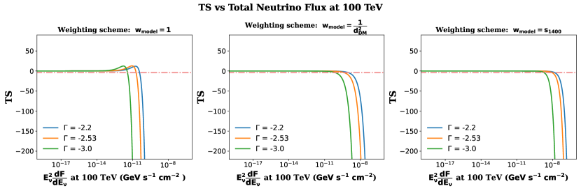
Figure 1: Plot of $TS$ (defined in Eq. 10) as a function of the total neutrino flux for pulsars in the ATNF catalog. using IceCube 10 year point source catalog. The left panel is when each pulsar is weighted equally and has been done with 3389 pulsars . The middle panel is when $w_{model}$ is scaled inversely according to the square of the distance and the rightmost panel is when $w_{model}$ is scaled to the pulsar flux density at 1400 Mhz. The latter two analyses have been done with 2374 pulsars where both distances and pulsar flux density were available. For each of the aforementioned analysis, we have considered three different neutrino spectral indices ($\Gamma$)

We now present the results of our analyses. We plot $TS$ as a function of the total neutrino flux at 100 TeV for the three weighting schemes (discussed in Sect. 10) in Fig 1. The graph of $TS$ as a function of the total neutrino flux reveals a marginal $w_{model}=1$, with a maximum value of $TS$ of around 13. These values occur at $E_{\nu}^{2}\dfrac{dF}{dE_{\nu}}$ equal to $1.8\times 10^{-11}$, $9.1\times 10^{-12}$, $1.7\times 10^{-12}$ for $\Gamma$=-2.2,-2.53, and -3, respectively. However, this is not a real signal and is likely an artificial artifact due to the large number of pulsars with $\delta=0^{\circ}$ where the effective area increases. To verify that is not a real signal, we redid this analysis for $w_{model}=1$ using 200 bootstrap tests, where we swapped the RA and declination of pulsars several times as well as applied an additive offset to the locations of pulsars. We found about two cases, where the value of $TS$ was greater than 10. Therefore prima-facie, we cannot interpret $\sqrt{TS}$ as a detection significance, since the $p$-value from our null tests is about 0.01, Furthermore, this slight excess of $TS$ disappears for the other two ansatzs used for $w_{model}$.

Therefore, we conclude that there is no statistically significant spatial excess when we do a spatial search by stacking all pulsars in the ATNF catalog.

We then proceed to calculate the upper limits on the total contribution by the pulsars at 95% c.l. At each energy, we calculate the total differential neutrino energy flux and plot their 95% c.l. upper Limits for which $TS=-3.84~{}$Zhou et al. (2021). We multiply the upper limits by a factor of three Li et al. (2022); Zhou et al. (2021) since are considering the flux due to the three different flavors of neutrinos.

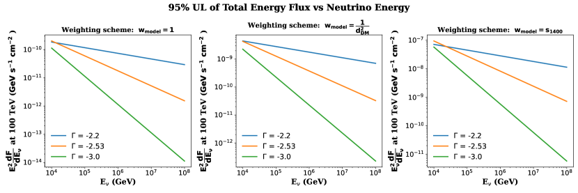
Figure 2: 95% c.l. upper limit on differential neutrino energy flux as a function of neutrino energy for three different values of $w_{model}$ and for three different spectral indices.

These upper limits on different neutrino energy flux as a function of neutrino energy for the three signal weighting schemes and three spectral indices (for each weighting scheme) can be found in Fig.  2.

V Conclusions

In a previous work Pasumarti and Desai (2022), we performed a single source unbinned likelihood analysis to determine the correlation between IceCube neutrinos and ATNF catalogie of pulsars. In this work, we extend that analysis by doing a stacking analysis Zhou et al. (2021); Li et al. (2022), in which the signal PDFs of all the sources are combined into a single stack. We then calculate $TS$ as a function of the total neutrino flux at 100 TeV for three different signal weighting schemes and three spectral indices for each weighting method. This plot for all the three signal weights can be found in 1. For $w_{model}$=1, where the signal from every pulsar is weighted equally, we find the maximum value of $TS$ of around 13. However, we verified using bootstrapping tests that this cannot be real signal, since we obtain the same value of $TS$ by swapping the declinations of the pulsars. Therefore, this excess cannot be due to a real signal. Furthermore, this excess vanishes for the other two signal weighting schemes where the contribution from every pulsar is scaled according to inverse square distance or $S_{1400}$. Therefore, we conclude that there is no statistically significant excess between the TeV neutrinos detected by IceCube and the stacked contribution from radio pulsars. We then calculate the 95% c.l. upper limits on the total neutrino flux of the pulsars in 2.

In the spirit of open science, we have made our analysis codes and the data used for our analysis publicly available. This can be found at https://github.com/DarkWake9/IceCube-Package

References

- Aartsen et al. (2013) M. G. Aartsen et al. (IceCube), Science 342, 1242856 (2013), eprint 1311.5238.
- Halzen (2023) F. Halzen, arXiv e-prints arXiv:2305.07086 (2023), eprint 2305.07086.
- Abbasi et al. (2021) R. Abbasi et al. (IceCube) (2021), eprint 2101.09836.
- Zhou et al. (2021) B. Zhou, M. Kamionkowski, and Y.-f. Liang, Phys. Rev. D 103, 123018 (2021), eprint 2103.12813.
- Hooper et al. (2019) D. Hooper, T. Linden, and A. Vieregg, JCAP 2019, 012 (2019), eprint 1810.02823.
- Luo and Zhang (2020) J.-W. Luo and B. Zhang, Phys. Rev. D 101, 103015 (2020), eprint 2004.09686.
- Smith et al. (2021) D. Smith, D. Hooper, and A. Vieregg, JCAP 2021, 031 (2021), eprint 2007.12706.
- Li et al. (2022) R.-L. Li, B.-Y. Zhu, and Y.-F. Liang, Phys. Rev. D 106, 083024 (2022), eprint 2205.15963.
- Luo and Zhang (2021) J.-W. Luo and B. Zhang, arXiv e-prints arXiv:2112.11375 (2021), eprint 2112.11375.
- Desai (2023) S. Desai, Journal of Physics G Nuclear Physics 50, 015201 (2023), eprint 2112.13820.
- Palladino and Vissani (2016) A. Palladino and F. Vissani, Astrophys. J. 826, 185 (2016), eprint 1601.06678.
- Vance et al. (2021) G. S. Vance, K. L. Emig, C. Lunardini, and R. A. Windhorst (2021), eprint 2108.01805.
- Desai (2022) S. Desai, JCAP 2022, 001 (2022), eprint 2202.12493.
- Pasumarti and Desai (2022) V. Pasumarti and S. Desai, JCAP 2022, 002 (2022), eprint 2210.12804.
- Helfand (1979) D. J. Helfand, Nature (London) 278, 720 (1979).
- Link and Burgio (2005) B. Link and F. Burgio, Phys. Rev. Lett. 94, 181101 (2005), eprint astro-ph/0412520.
- Fang et al. (2012) K. Fang, K. Kotera, and A. V. Olinto, Astrophys. J. 750, 118 (2012), eprint 1201.5197.
- Fang et al. (2016) K. Fang, K. Kotera, K. Murase, and A. V. Olinto, JCAP 2016, 010 (2016), eprint 1511.08518.
- Manchester et al. (2005) R. N. Manchester, G. B. Hobbs, A. Teoh, and M. Hobbs, Astron. J. 129, 1993 (2005), eprint astro-ph/0412641.
- Braun et al. (2010) J. Braun, M. Baker, J. Dumm, C. Finley, A. Karle, and T. Montaruli, Astroparticle Physics 33, 175 (2010), eprint 0912.1572.
- Yao et al. (2017) J. M. Yao, R. N. Manchester, and N. Wang, Astrophys. J. 835, 29 (2017), eprint 1610.09448.
- Desai (2016) S. Desai, Astrophysics and Space Sciences 361, 138 (2016), eprint 1512.05962.
- Wilks (1938) S. S. Wilks, The annals of mathematical statistics 9, 60 (1938).
- Wolf (2019) M. Wolf, in 36th International Cosmic Ray Conference (ICRC2019) (2019), vol. 36 of International Cosmic Ray Conference, p. 1035, eprint 1908.05181.