ColdNAS: Search to Modulate for User Cold-Start Recommendation
Abstract.
Making personalized recommendation for cold-start users, who only have a few interaction histories, is a challenging problem in recommendation systems. Recent works leverage hypernetworks to directly map user interaction histories to user-specific parameters, which are then used to modulate predictor by feature-wise linear modulation function. These works obtain the state-of-the-art performance. However, the physical meaning of scaling and shifting in recommendation data is unclear. Instead of using a fixed modulation function and deciding modulation position by expertise, we propose a modulation framework called ColdNAS for user cold-start problem, where we look for proper modulation structure, including function and position, via neural architecture search. We design a search space which covers broad models and theoretically prove that this search space can be transformed to a much smaller space, enabling an efficient and robust one-shot search algorithm. Extensive experimental results on benchmark datasets show that ColdNAS consistently performs the best. We observe that different modulation functions lead to the best performance on different datasets, which validates the necessity of designing a searching-based method. Codes are available at https://github.com/LARS-research/ColdNAS.
1. Introduction
Recommendation systems (RSs) (Resnick and Varian, 1997) target at providing suggestions of items that are most pertinent to a particular user, such as movie recommendation (Harper and Konstan, 2015) and book recommendation (Ziegler et al., 2005). Nowadays, RSs are abundant online, offering enormous users convenient ways to shopping regardless of location and time, and also providing intimate suggestions according to their preferences. However, user cold-start recommendation (Schein et al., 2002) remains a severe problem in RSs. On the one hand, the users in RSs follow long tail effect (Park and Tuzhilin, 2008), some users just have a few interaction histories. On the other hand, new users are continuously emerging, who naturally have rated a few items in RSs. Such a problem is even more challenging as modern RSs are mostly built with over-parameterized deep networks, which needs a huge amount of training samples to get good performance and can easily overfit for cold-start users (Volkovs et al., 2017).
User cold-start recommendation problem can naturally be modeled as a few-shot learning problem (Wang et al., 2020), which targets at quickly generalize to new tasks (i.e. personalized recommendation for cold-start users) with a few training samples (i.e. a few interaction histories). A number of works (Lee et al., 2019; Dong et al., 2020; Lu et al., 2020; Yu et al., 2021; Wang et al., 2021) adopt the classic gradient-based meta-learning strategy called model-agnostic meta-learning (MAML) (Finn et al., 2017), which learns a good initialized parameter from a set of tasks and adapts it to a new task by taking a few steps of gradient descent updates on a limited number of labeled samples. This line of models has demonstrated high potential of alleviating user cold-start problem. However, gradient-based meta-learning strategy require expertise to tune the optimization procedure to avoid over-fitting. Besides, the inference time can be long.
Instead of adapting to each user by fine-tuning via gradient descent, another line of works uses hypernetworks (Ha et al., 2017) to directly map user interaction history to user-specific parameters (Dong et al., 2020; Lin et al., 2021; Feng et al., 2021; Pang et al., 2022). These modulation-based methods consist of embedding layer, adaptation network and predictor. The adaptation network generates user-specific parameters, which are used to modulate the predictor in the form of a modulation function. Particularly, they all adopt feature-wise linear modulation function (FiLM) (Perez et al., 2018), which modulates the representation via scaling and shifting based on the conditioning information, to modulate the user cold-start models to obtain user-specific representation. Although FiLM has been proved to be highly effective in on images (Requeima et al., 2019) and graphs such molecules and protein-protein interaction graphs (Brockschmidt, 2020), applying scaling and shifting on user interaction history has rather obscure physical meaning. Moreover, choosing where to modulate is hard to decide. Existing works modulate different parts of the model, such as last layers of the decoder (Lin et al., 2021) and most layers in the model (Pang et al., 2022). How to modulate well for different users, and how to choose the right functions at the right positions to modulate, are still open questions.
In this paper, we propose ColdNAS to find appropriate modulation structure for user cold-start problem by neural architecture search (NAS). Although NAS methods have been applied in RSs (Gao et al., 2021a; Xie et al., 2021), the design of NAS methods are problem-specific. For user cold-start problem, it is still unknown how to (i) design a search space that can cover effective cold-start models with good performance for various datasets, and (ii) design an efficient and robust search algorithm. To solve the above challenges, we design a search space of modulation structure, which can cover not only existing modulation-based user cold-start models, but also contain more flexible structures. We theoretically prove that the proposed search space can be transformed to an equivalent space, where we search efficiently and robustly by differentiable architecture search. Our main contributions are summarized as follows:
-
•
We propose ColdNAS, a modulation framework for user cold-start problem. We use a hypernetwork to map each user’s history interactions to user-specific parameters which are then used to modulate the predictor, and formulate how to modulate and where to modulate as a NAS problem.
-
•
We design a search space of modulation structure, which can cover not only existing modulation-based user cold-start models, but also contain more expressive structures. As this search space can be large to search, we conduct search space transformation to transform the original space to an equivalent but much smaller space. Theoretical analysis is provided to validate its correctness. Upon the transformed space, we then can search efficiently and robustly by differentiable architecture search algorithm.
-
•
We perform extensive experiments on benchmark datasets for user cold-start problem, and observe that ColdNAS consistently obtains the state-of-the-art performance. We also validate the design consideration of search spaces and algorithms, demonstrating the strength and reasonableness of ColdNAS.
2. Related Works
2.1. User Cold-Start Recommendation
Making personalized recommendation for cold-start users is particular challenging, as these users only have a few interaction histories (Schein et al., 2002). In the past, collaborative filtering (CF)-based (Koren, 2008; Sedhain et al., 2015; He et al., 2017) methods, which make predictions by capturing interactions among users and items to represent them in low-dimensional space, obtain leading performance in RSs. However, these CF-based methods make inferences only based on the user’s history. They cannot handle user cold-start problem. To alleviate the user cold-start problem, content-based methods leverage user/item features (Schein et al., 2002) or even user social relations (Lin et al., 2013) to help to predict for cold-start users. The recent deep model DropoutNet (Volkovs et al., 2017) trains a neural network with dropout mechanism applied on input samples and infers the missing data. However, it is hard to generalize these content-based methods to new users, which usually requires model retraining.
A recent trend is to model user cold-start problem as a few-shot learning problem (Wang et al., 2020). The resultant models learn the ability to quickly generalize to recommend for new users with a few interaction histories. Most works mainly follow the classic gradient-based meta-learning strategy MAML (Finn et al., 2017), which first learns a good initialized parameter from training tasks, then locally update the parameter on the provided interaction history by gradient descent. In particular, existing works consider different directions to improve the performance: MeLU (Lee et al., 2019) selectively adapts model parameters to the new task in the local update stage, MAMO (Dong et al., 2020) introduces external memory to guide the model to adapt, MetaHIN (Lu et al., 2020) uses heterogeneous information networks to leverage the rich semantics between users and items, REG-PAML (Yu et al., 2021) proposes to use user-specific learning rate during local update, and PAML (Wang et al., 2021) leverages social relations to share information among similar users. While these approaches can adapt models to training data, they are computationally inefficient at test-time, and usually require expertise to tune the optimization procedure to avoid over-fitting.
2.2. Neural Architecture Search
Neural architecture search (NAS) targets at finding an architecture with good performance without human tuning (Hutter et al., 2019). Recently, NAS methods have been applied in RSs. SIF (Yao et al., 2020a) searches for interaction function in collaborative filtering, AutoCF (Gao et al., 2021b) further searches for basic components including input encoding, embedding function, interaction function, and prediction function in collaborative filtering. AutoFIS (Liu et al., 2020), AutoCTR (Song et al., 2020) and FIVES (Xie et al., 2021) search for effective feature interaction in click-through rate prediction. AutoLoss (Zhao et al., 2021) searches for loss function in RSs. Due to different problem settings, search spaces needs to problem-specific and cannot be shared or transferred. Therefore, none of these works can be applied for user cold-start recommendation problem. To search efficiently on the search space, one can choose reinforcement learning methods (Baker et al., 2017), evolutionary algorithms (Real et al., 2019), and one-shot differentiable architecture search algorithms (Liu et al., 2019; Pham et al., 2018; Yao et al., 2020b). Among them, one-shot differentiable architecture search algorithms have demonstrated higher efficiency. Instead of training and evaluating different models like classical methods, they optimize only one supernet where the model parameters are shared across the search space and co-adapted.
3. Proposed Method
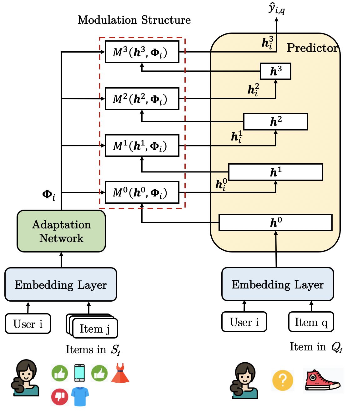
In this section, we present the details of ColdNAS, whose overall architecture is shown in Figure 1. In the sequel, we first provide the formal problem formulation of user cold-start problem (Section 3.1). Then, we present our search space and theoretically show how to transform it (Section 3.2). Finally, we introduce the search algorithm to search for a good user cold-start model (Section 3.3).
3.1. Problem Formulation
Let user set be denoted , where each user is associated with user features. The feature space is shared across all users. Let item set be denoted where each item is also associated with item features. When a user rates an item , the rating is denoted . In user cold-start recommendation problem, the focus is to make personalized recommendation for user who only has rated a few items.
Following recent works (Bharadhwaj, 2019; Lu et al., 2020; Lin et al., 2021), we model the user cold-start recommendation problem as a few-shot learning problem. The target is to learn a model from a set of training user cold-start tasks and generalize to provide personalized recommendation for new tasks. Each task corresponds to a user , with a support set containing existing interaction histories and a query set containing interactions to predict. and are the number of interactions in . and are small.
3.2. Search Space
Existing modulation-based user cold-start works can be summarized into the following modulation framework consisting of three parts, i.e., embedding layer, adaptation network and predictor, as plotted in Figure 1.
-
•
The embedding layer with parameter embeds the categorical features from users and items into dense vectors, i.e., .
-
•
The adaptation network with parameter takes the support set for a specific user as input and generates user-specific adaptive parameters, i.e.,
(1) where is the number of adaptive parameter groups for certain modulation structure.
-
•
The predictor with parameter takes user-specific parameters and from the query set as input, and generate predictions by
(2)
Comparing with classical RS models, the extra adaptation network is introduced to handle cold-start users. To make personalized recommendation, for each , the support set is first mapped to user-specific parameter by (1). Then taking the features of target item , user features , and the , prediction is made as (2). Subsequently, how to use the user-specific parameter to change the prediction process in (2) can be crucial to the performance. Usually, a multi-layer perception (MLP) is used as (Cheng et al., 2016; He et al., 2017; Lin et al., 2021). Assume a -layer MLP is used and denotes its output from the th layer, and let for notation simplicity. For the th user, is modulated as
| (3) | ||||
| (4) |
where is the modulation function, and are learnable weights at the th layer. This controls how is personalized w.r.t. the th user. The recent TaNP (Lin et al., 2021) directly lets in (3) adopt the form of FiLM for all MLP layers:
| (5) |
FiLM applies a feature-wise affine transformation on the intermediate features, and has been proved to be highly effective in other domains (Requeima et al., 2019; Brockschmidt, 2020). However, users and items can have diverse interaction patterns. For example, both the inner product and summation have been used in RS to measure the preference of user over items (Koren, 2008; Hsieh et al., 2017).
In order to find the appropriate modulation function, we are motivated to search for different recommendation tasks. We design the following space for :
| (6) |
where ’ are defined as
They are all commonly used simple dimension-preserving binary operations. We choose them to avoid the resultant being too complex, which can easily overfit for cold-start users.
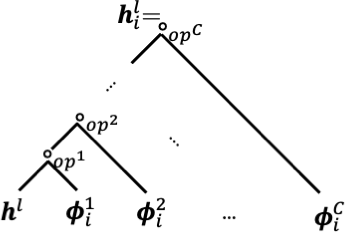
The search space in (6) can be viewed as a binary tree, as shown in Figure 2(a). Since can be different for each layer, the size of this space is . A larger leads to a larger search space, which has higher potential of containing appropriate modulation function but is also more challenging to search effectively.
3.3. Search Strategy
We aim to find an efficient and practicable search algorithm on the proposed search space. However, the search space can be very large, and differentiable NAS methods are known to be fragile on large spaces (Yu et al., 2019). In the sequel, we propose to first transform the original search space to an equivalent but much smaller space, as shown in Figure 2(a), where the equivalence is inspired by some similarities between the operations and the expressiveness of deep neural networks. On the transformed space, we design a supernet structure to conduct efficient and robust differentiable search.
3.3.1. Search Space Transformation
Though the aforementioned search space can be very large, we can transform it to an equivalent space of size which is invariant with , as proved in Proposition 3.1111The proof is in Appendix B. below.
Proposition 3.1 (Search Space Transformation).
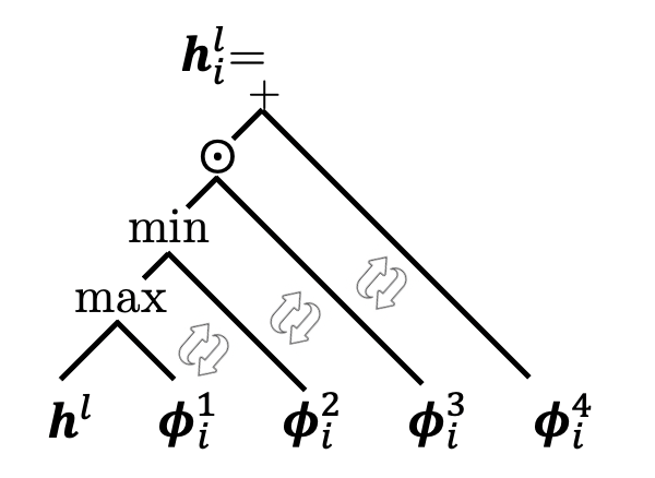
Assume the adaptation network is expressive enough. Any with a form of (6) where , is any non-negative integer, and , can be represented as
| (7) |
and the above four operations are permutation-invariant.
The intuitions are as follows. First, operations in can be divided into four groups: . Then, with mild assumption on adaptation network, we can prove two important properties: (i) inner-group consistence: operations that in the same group can be associated; and (ii) inter-group permutation-invariance: operations that are not in the same group are permutation-invariant which means any two operations can switch with another. Thus, we can recurrently commute operations until operations in the same group are neighbors, and associate operations in the four groups respectively.
Remark 1.
Note that due to the universal approximation ability of deep network (Hornik et al., 1989), the assumption in this proposition can be easily satisfied. For example, we implement based on two-layer MLP in experiments (see Appendix A.2), which can already ensure a good performance (see Section 4.3.3). After the transformation, the space in (7) also spans a permutation-invariant binary tree, as plotted in Figure 2(b). Such a space can be significantly smaller than the original one, as explained in Remark 2 below.
Remark 2.
The space transformation plays an essential role in ColdNAS, Table 1 helps to better understand to what extent the proposition can help reduce the search space, we take layer number and the ratio is calculated as .
| 1 | 2 | 3 | 4 | 5 | 6 | |
|---|---|---|---|---|---|---|
| Ratio |
Note that when , the transformation will not lead to a reduction on the space. However, such a case is not meaningful as it suffers from poor performance due to lack of flexibility for the modulation function (see Section 4.3.2). The transformed spaces enable efficient and robust differentiable search, via reducing the number of architecture parameter from to . Meanwhile, the space size is transformed from to , which is a reduction for any .
3.3.2. Construction of the Supernet
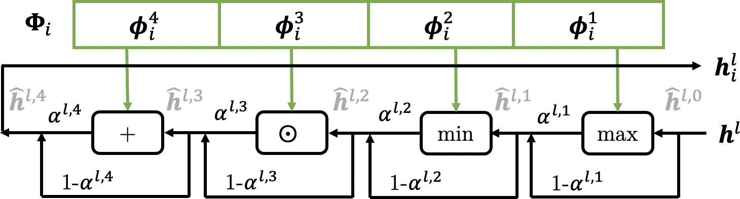
For each , since there are operations at most and they are permutation-invariant, we only need to decide whether to take the operation or not by any order. We search by introducing differentiable parameters to weigh the operations and optimize the weights. For the th layer of the predictor, we have
| (8) |
where is a weight to measure operation in , and . For notation simplicity, we let . We construct the supernet by replacing (3) with (8), i.e., replacing every in red dotted lines in Figure 1 with the structure shown in Figure 2 (c).
3.3.3. Complete Algorithm
The complete algorithm is summarized in Algorithm 1. We first optimize the supernet and make selection to determine the structure, then reconstruct the model with determined structure and retrain it to inference.
Benefited from the great reduction brought by the space transformation, while conventional differentiable architecture search (Liu et al., 2019) optimizes the supernet w.r.t. the bilevel objective with the upper-level variable and lower-level variable :
| (9) |
where and represent the loss obtained on validation set and training set respectively, we only need to optimize the supernet w.r.t. objective only, in an end-to-end manner by episodic training. For every task , we first input to the adaptation network to generate by (1), and then for every item , we take and as input of the predictor and make prediction by (2). Then, we use mean squared error (MSE) between the prediction and true label as loss function:
| (10) |
and . We update all parameters by gradient descent. Once the supernet converges, we determine all s jointly by keeping the operation corresponding to the Top- largest values among the values in . We then retrain the model to obtain the final user cold-start model with searched modulation structure. During inference, a new set of tasks is given, which is disjoint from . For , we take the whole and as input to the trained model to obtain prediction for each item .
3.4. Discussion
Existing works in space transformation can be divided into three types. One is using greedy search strategy (Gao et al., 2021a). Methods of this kind explore different groups of architectures in the search space greedily. Thus, they fail to explore the full search space and can easily fall into bad local optimal. Another is mapping the search space into a low-dimensional one. For examples, using auto-encoder (Luo et al., 2018) or sparse coding (Yang et al., 2020). However, these types of methods do not consider special properties of the search problem, e.g., the graph structure of the supernet. Thus, the performance ranking of architectures may suffer from distortion in the low-dimensional space. ColdNAS belongs to the third type, which is to explore architecture equivalence in the search space. The basic idea is that if we can find a group of architectures that are equivalent with each other, then evaluation any one of them is enough for all architectures in the same group. This type of methods is problem-specific. For example, perturbation equivalence for matrices is explored in (Zhang et al., 2023), morphism of networks is considered in (Jin et al., 2019). The search space of ColdNAS is designed for modulation structures in cold-start problem, which has not been explored before. We theoretically prove the equivalence between the original space and the transformed space, which then significantly reduces the space size (Remark 2). Other methods for general space reduction cannot achieve that.
| Dataset | Metric | DropoutNet | MeLU | MetaCS | MetaHIN | MAMO | TaNP | ColdNAS-Fixed | ColdNAS |
|---|---|---|---|---|---|---|---|---|---|
| MovieLens | MSE | ||||||||
| MAE | |||||||||
| BookCrossing | MSE | ||||||||
| MAE | |||||||||
| Last.fm | MSE | ||||||||
| MAE | |||||||||
| MovieLens | ||||
|---|---|---|---|---|
| BookCrossing | ||||
| Last.fm | ||||
| ColdNAS-Fixed |
4. Experiments
We perform experiments on three benchmark datasets with the aim to answer the following research questions:
-
•
RQ1: What is the modulation structure selected by ColdNAS and how does ColdNAS perform in comparison with the state-of-the-art cold-start models?
-
•
RQ2: How can we understand the search space and algorithm of ColdNAS?
-
•
RQ3: How do hyperparameters affect ColdNAS?
Results are averaged over five runs.
4.1. Datasets
We use three benchmark datasets (Table 4): (i) MovieLens (Harper and Konstan, 2015): a dataset containing 1 million movie ratings of users collected from MovieLens, whose features include gender, age, occupation, Zip code, publication year, rate, genre, director and actor; (ii) BookCrossing (Ziegler et al., 2005): a collection of users’ ratings on books in BookCrossing community, whose features include age, location, publish year, author, and publisher; and (iii) Last.fm: a collection of user’s listening count of artists from Last.fm online system, whose features only consist of user and item IDs. Following Lin et al. (2021), we generate negative samples for the query sets in Last.fm.
| Dataset | # User (Cold) | # Item | # Rating | # User Feat. | # Item Feat. |
|---|---|---|---|---|---|
| MovieLens | 6040 (52.3%) | 3706 | 1000209 | 4 | 5 |
| BookCrossing | 278858 (18.6%) | 271379 | 1149780 | 2 | 3 |
| Last.fm | 1872 (15.3%) | 3846 | 42346 | 1 | 1 |
Data Split
Following Lin et al. (2021), the ratio of is set as . is used to judge the convergence of supernet. contain no overlapping users. For MovieLens and Last.fm, we keep any user whose interaction history length lies in . Each support set contains randomly selected interactions of a user, and query set contains the rest interactions of the same user. As for BookCrossing with severe long-tail distribution of user-item interactions, we particularly put any user whose interaction history length lies in into . Then, we divide users with interaction history length in into , and to be put in , , respectively. The proportion of cold users in each dataset is also shown in Table 4. Then, we randomly select half of each user’s interaction history as support set and take the rest as query set.
Evaluation Metric
Following (Lee et al., 2019; Pang et al., 2022), we evaluate the performance by mean average error (MAE), mean squared Error (MSE), normalized discounted cumulative gain and . MAE and MSE evaluate the numerical gap between the prediction and the ground-truth rating, lower value is better. For and , the higher value is better, representing the proportion between the discounted cumulative gain of the predicted item list and the ground-truth list.
4.2. Performance Comparison (RQ1)
We compare ColdNAS with the following representative user cold-start methods: (i) traditional deep cold-start model DropoutNet (Volkovs et al., 2017) and (ii) FSL based methods include MeLU (Lee et al., 2019), MetaCS (Bharadhwaj, 2019), MetaHIN (Lu et al., 2020), MAMO (Dong et al., 2020), and TaNP (Lin et al., 2021). We run the public codes provided by the respective authors. PNMTA (Pang et al., 2022), CMML (Feng et al., 2021), PAML (Wang et al., 2021) and REG-PAML (Yu et al., 2021) are not compared due to the lack of public codes. We choose a 4-layer predictor, more details of our model and parameter setting are provided in Appendix C.1. We also compare with a variant of ColdNAS called ColdNAS-Fixed, which uses the fixed FiLM function in (5) at every layer rather than our searched modulation function.
Table 2 shows the overall user-cold start recommendation performance for all methods. We can see that ColdNAS significantly outperforms the others on all the datasets and metrics. Among all compared baselines, DropoutNet performs the worst as it is not a few-shot learning method that the model has no ability to adapt to different users. Among meta-learning based methods, MeLU, MetaCS, MetaHIN and MAMO adopt gradient-based meta-learning strategy, which may suffer from overfitting during local-updates. In contrast, TaNP and ColdNAS learn to generate user-specific parameters to guide the adaptation. TaNP uses a fixed modulation structure which may not be optimal for different datasets, while ColdNAS automatically finds the optimal structure. Further, the consistent performance gain of ColdNAS over ColdNAS-Fixed validates the necessity of searching modulation structure to fit datasets instead of using a fixed one.
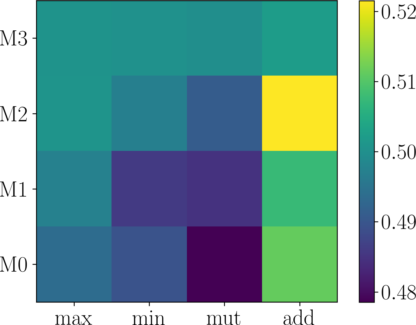
Table 3 shows the searched modulation structures. We find that the searched modulation structures are different across the datasets. No modulation should be taken at the last layer, as directly use user-specific preference possibly leads to overfitting. Note that all the operations in the transformed search space have been selected at least once, which means all of them are helpful.
Comparing time consumption to other cold-start models, ColdNAS only additionally optimizes a supernet with the same objective and comparable size. Table 5 shows the clock time taken by ColdNAS and TaNP which obtains the second-best in Table 2. As can be observed, the searching in ColdNAS is very efficient, as it is only slightly more expensive than retraining.
| Clock time (min) | MovieLens | BookCrossing | Last.fm | |
|---|---|---|---|---|
| TaNP | 15.5 | 44.2 | 4.1 | |
| ColdNAS | Search | 16.2 | 45.5 | 3.9 |
| Retrain | 12.7 | 35.5 | 3.5 | |
4.3. Searching in ColdNAS (RQ2)
4.3.1. Choice of Search Strategy
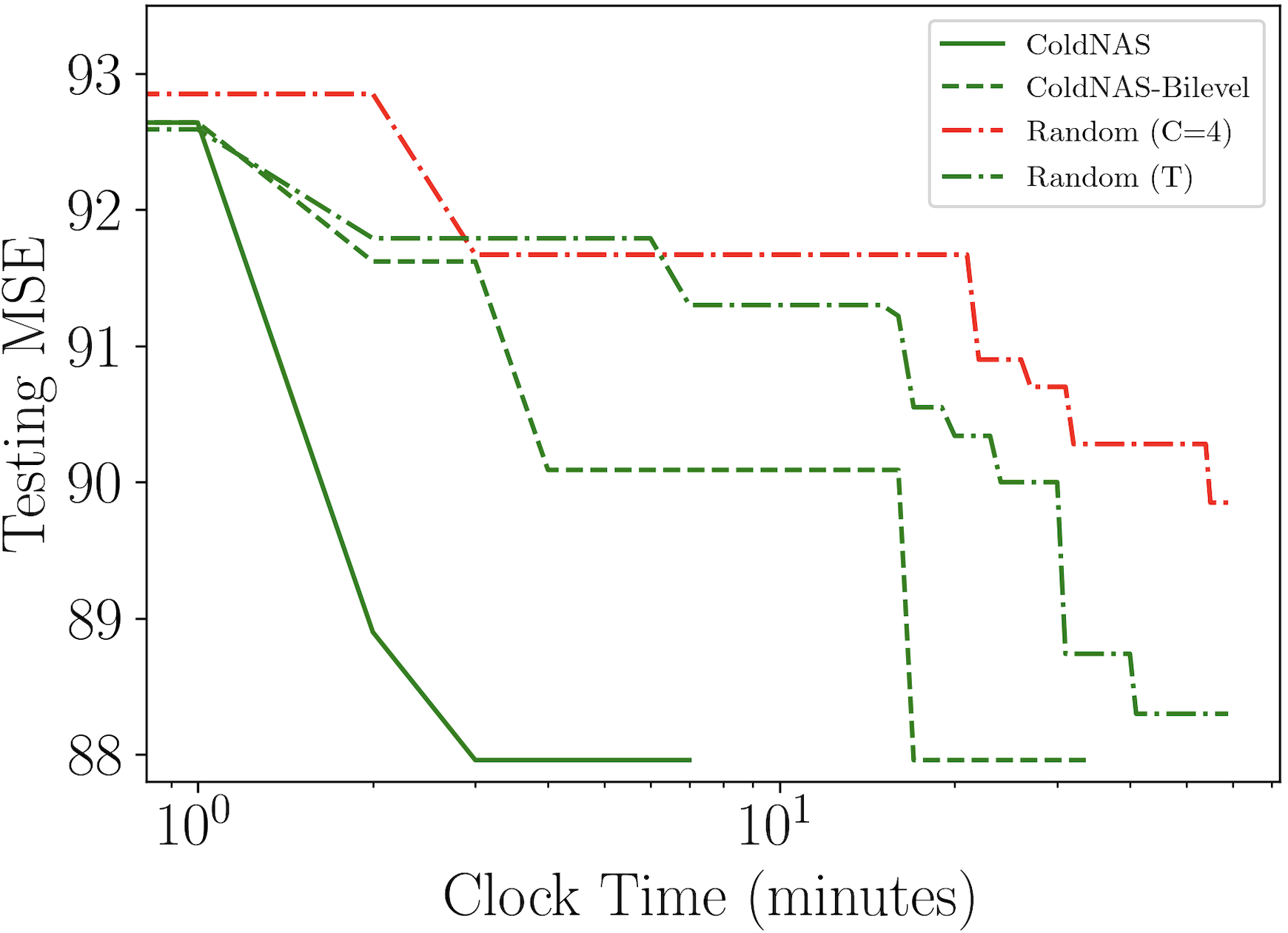
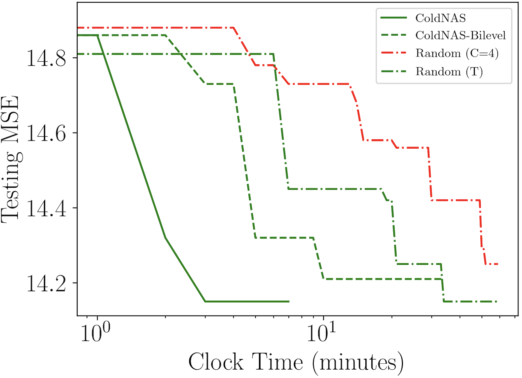
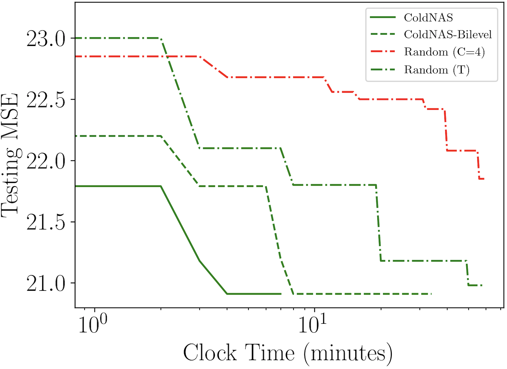
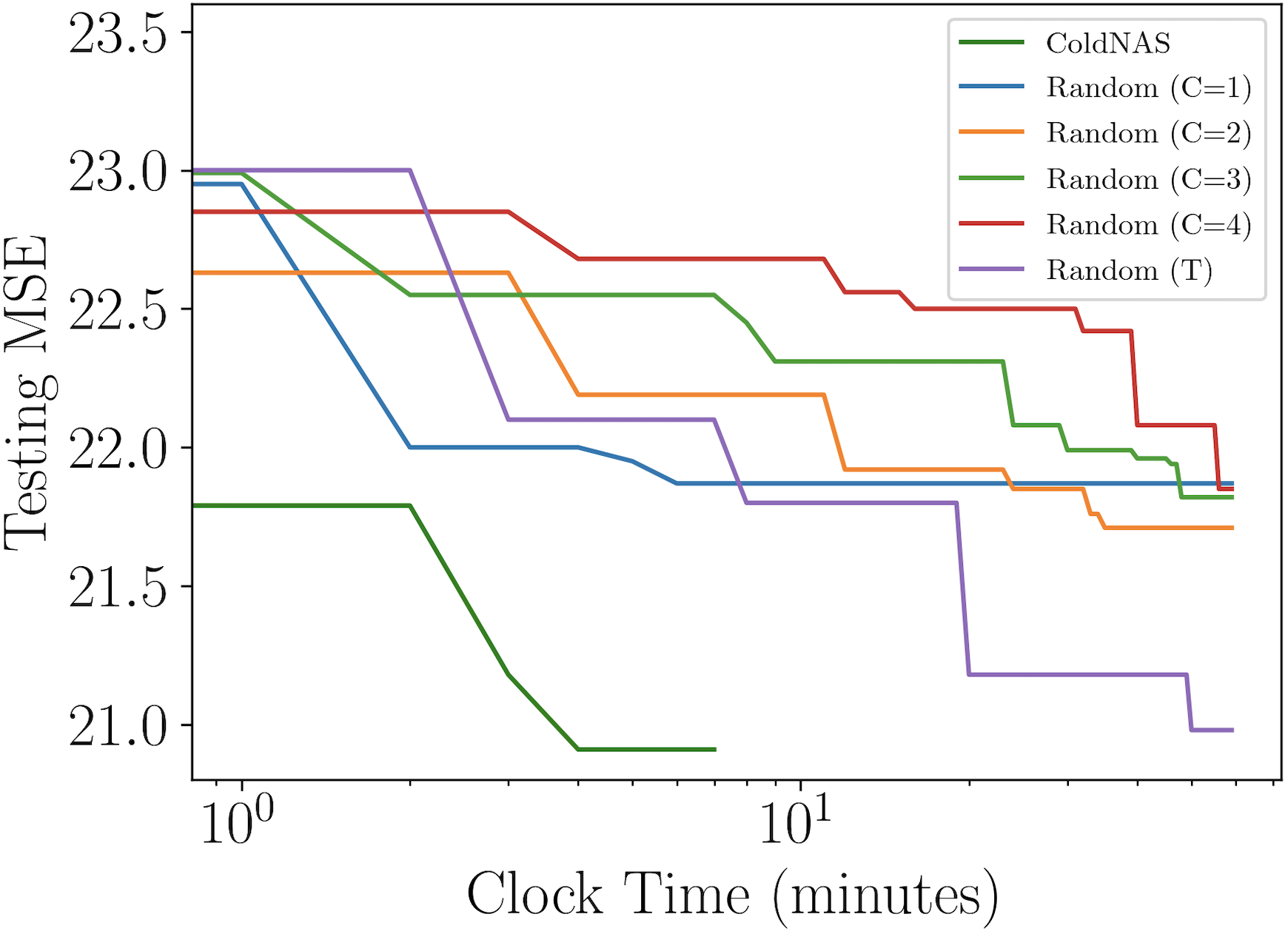
In ColdNAS, we optimize (10) by gradient descent. In this section, we compare ColdNAS with other search strategies to search the modulation structure, including Random () which conducts random search (Bergstra and Bengio, 2012) on the original space with operation number in each , Random (T) which conducts random search (Bergstra and Bengio, 2012) on the transformed space, ColdNAS-Bilevel which optimizes the supernet with the bilevel objective 9. For random search, we record its training and evaluation time. For ColdNAS and ColdNAS-bilevel, we sample the architecture parameter of the supernet and retrain from scratch, and exclude the time for retraining and evaluation. Figure 3 shows the performance of the best searched architecture. One can observe that searching on the transformed space allows higher efficiency and accuracy, comparing Random (T) to Random (). In addition, differentiable search on the supernet structure has brought more efficiency, as both ColdNAS and ColdNAS-Bilevel outperform random search. ColdNAS and ColdNAS-Bilevel converge to similar testing MSE, but ColdNAS is faster. This validates the efficacy of directly using gradient descent on all parameters in ColdNAS.
4.3.2. Necessity of Search Space Transformation
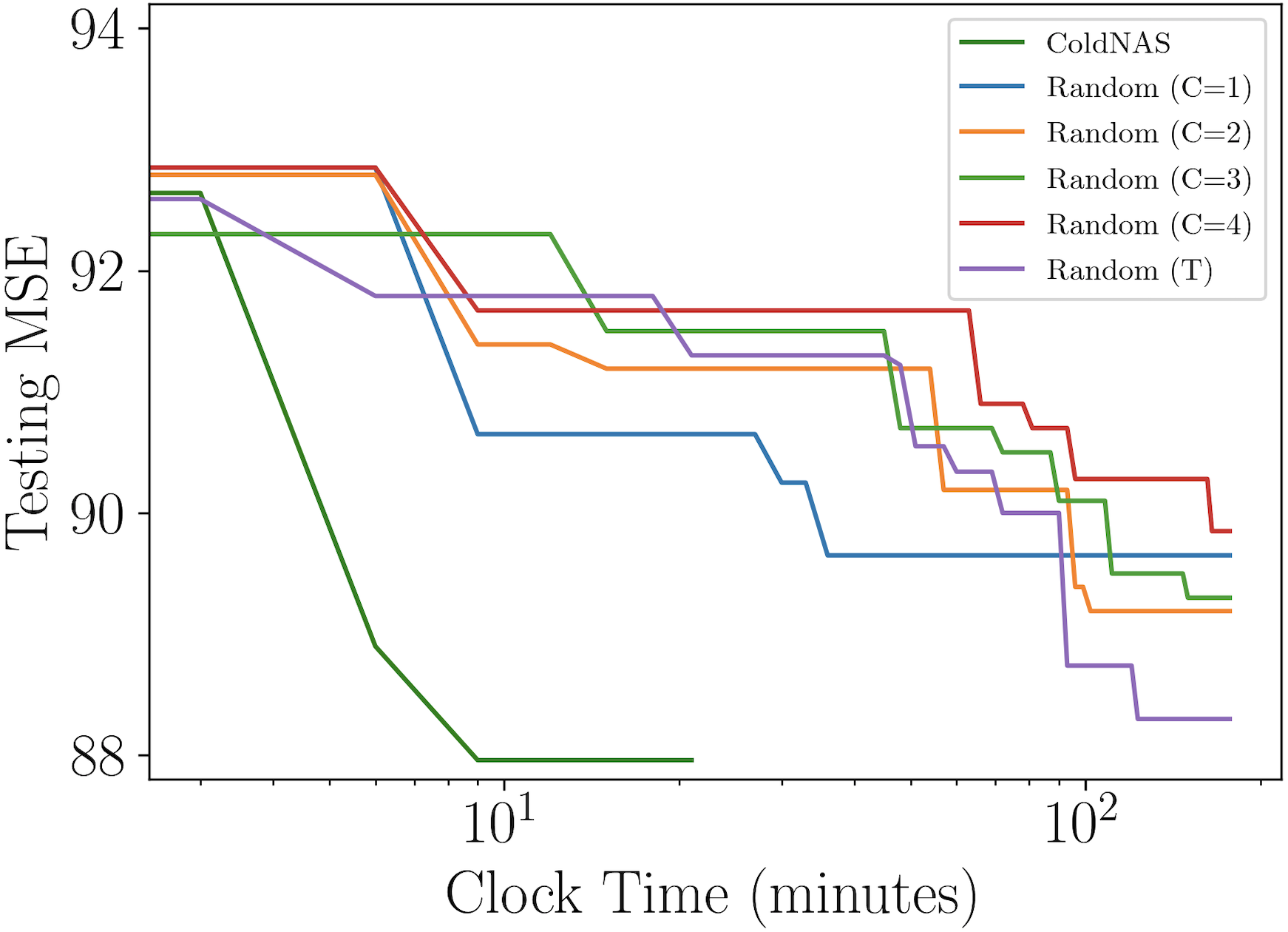
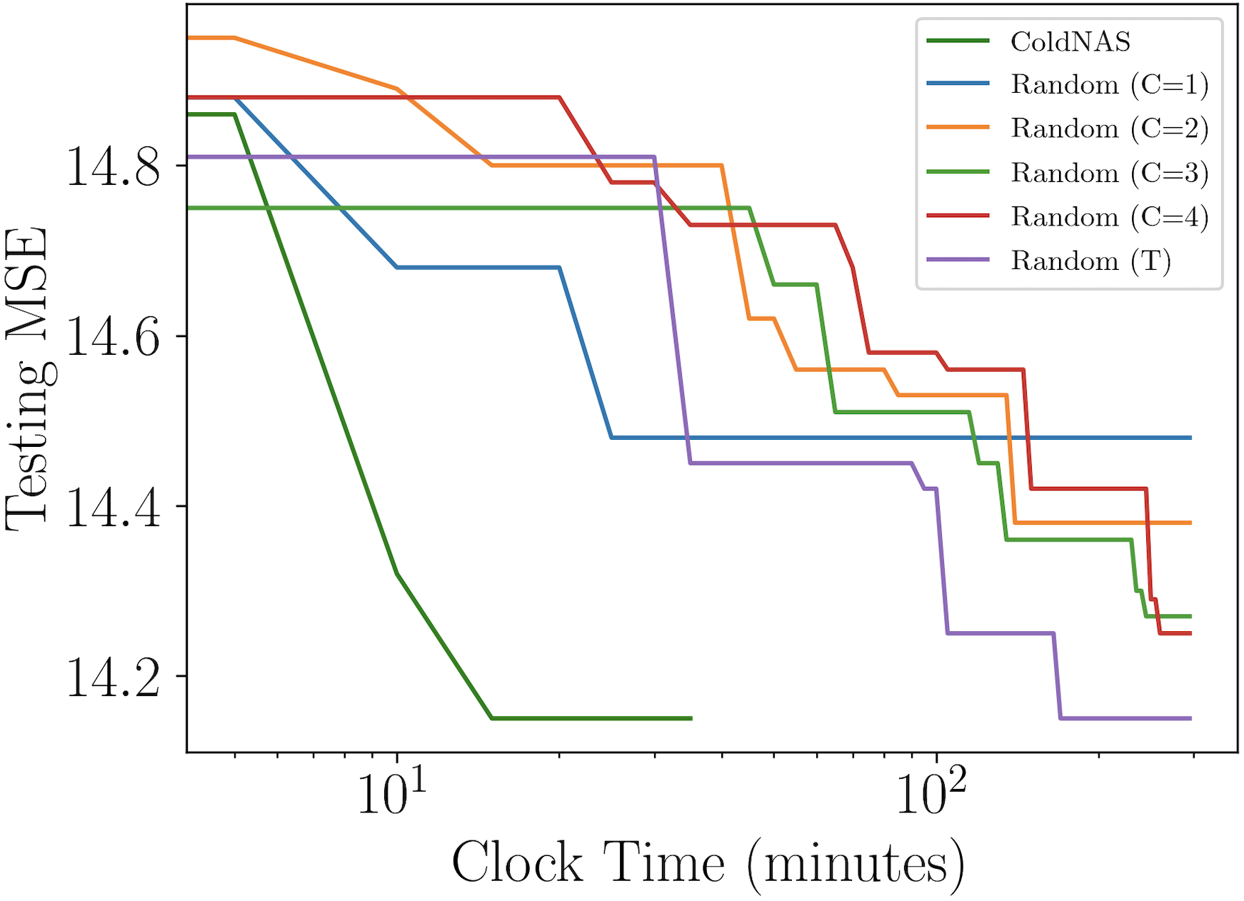
Now that the search algorithm has been chosen, we now particularly examine the necessity of search space transformation in terms of time and performance. As shown in Table 1, a larger which constrains the number of operations will lead to a larger original space. And the space reduction ratio grows exponentially along with the original space size. Figure 4 plots the testing MSE vs clock time of random search on original spaces of different size (Random ()), random search on transformed space (Random (T)), and our ColdNAS. When is small, modulation functions would not be flexible enough, though it is easy to find the optimal candidate in this small search space. When is large, the search space is large, where random search would be too time-consuming to find a good modulation structure. In contrast, the transformed search space has a consistent small size, and is theoretically proved to be equal to the space with any . As can be seen, both Random (T) and ColdNAS can find good structure more effective than Random (), and ColdNAS searches the fastest via differentiable search.
4.3.3. Understanding Proposition 3.1
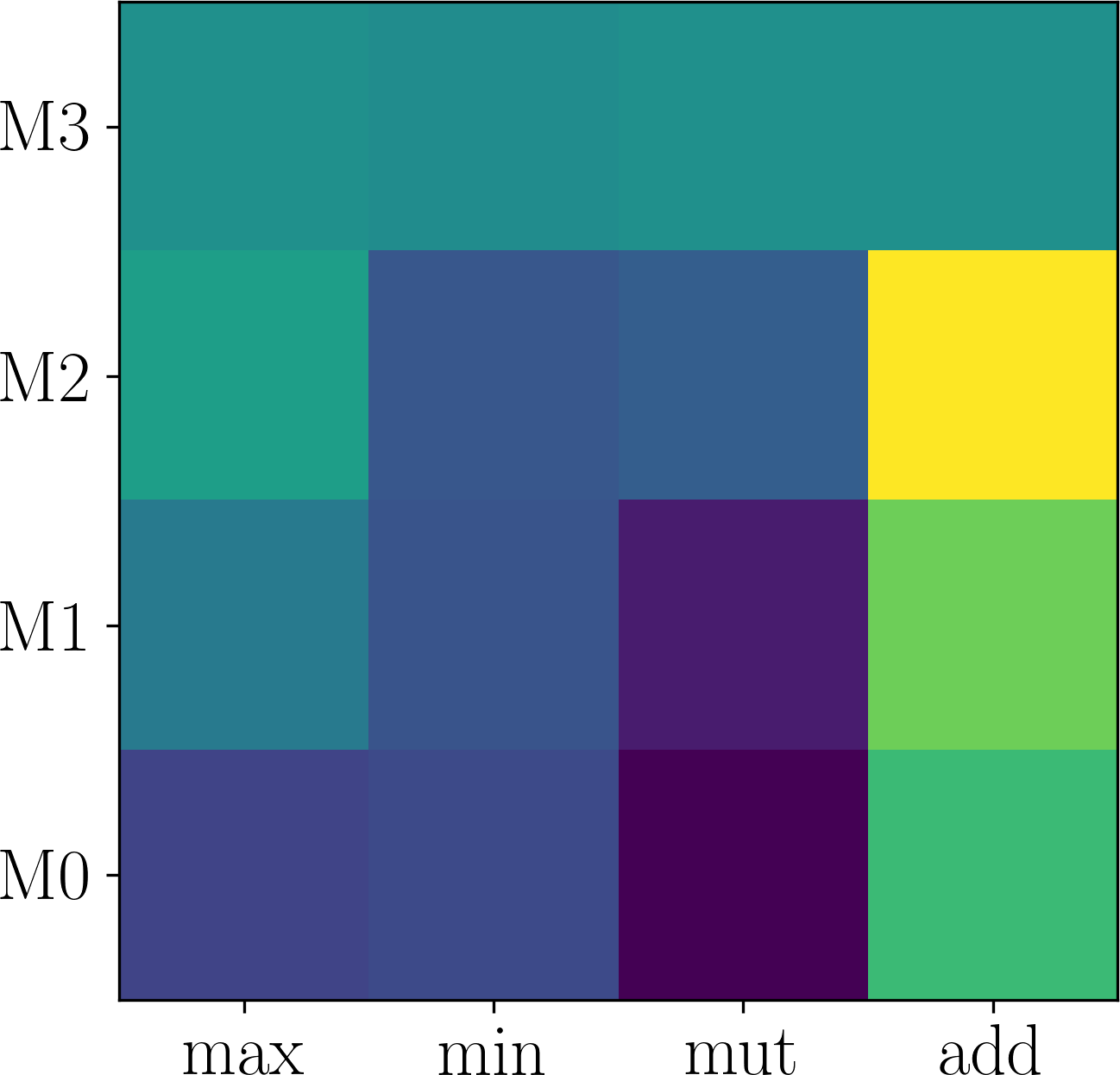
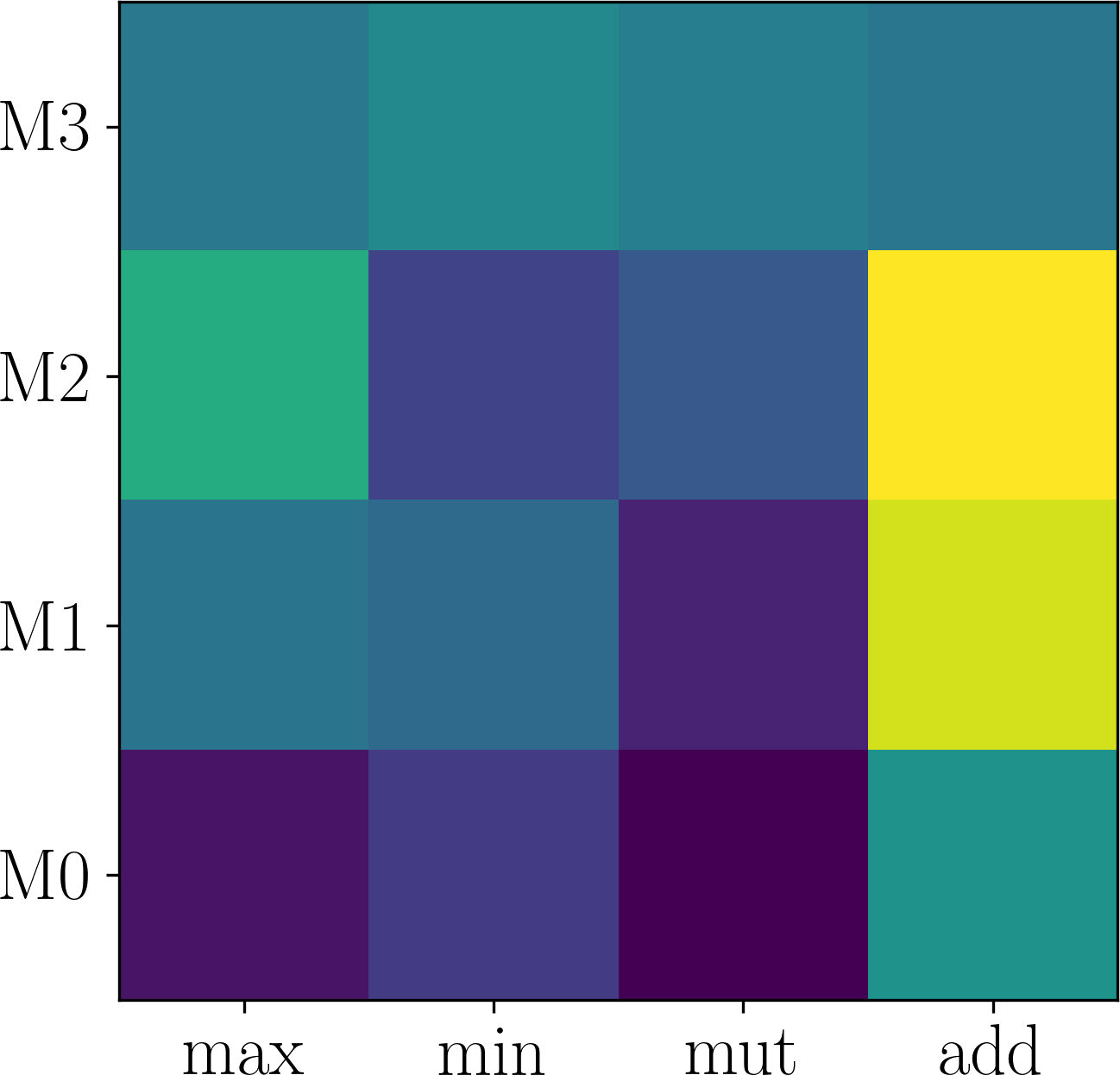
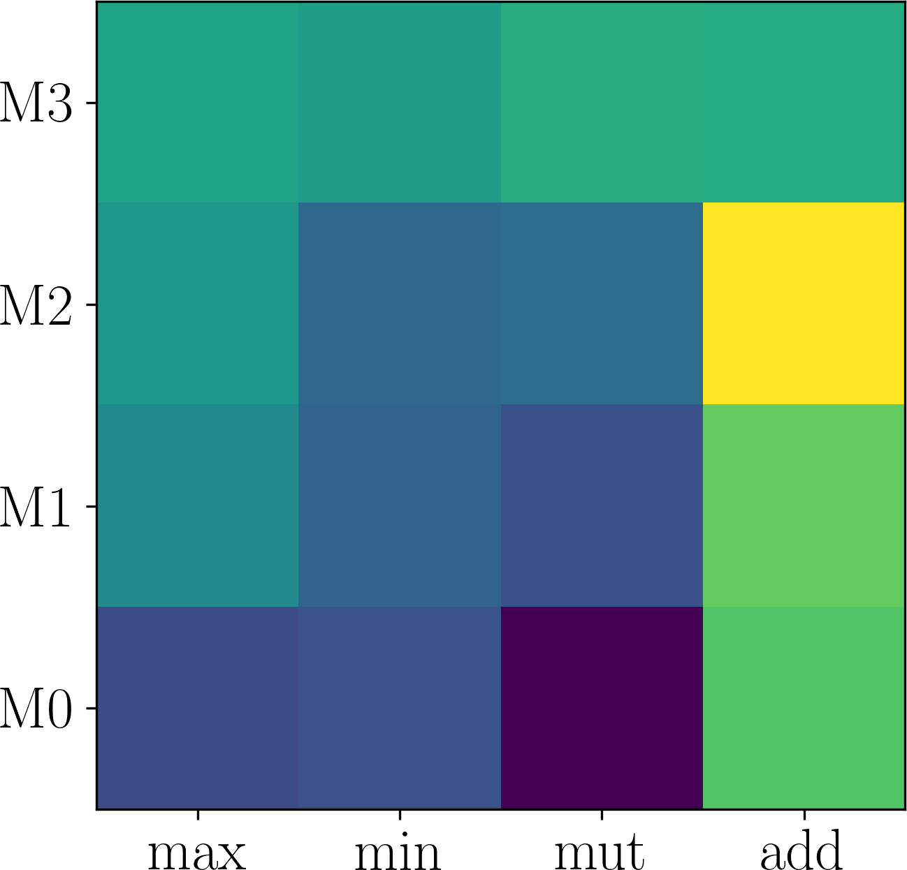
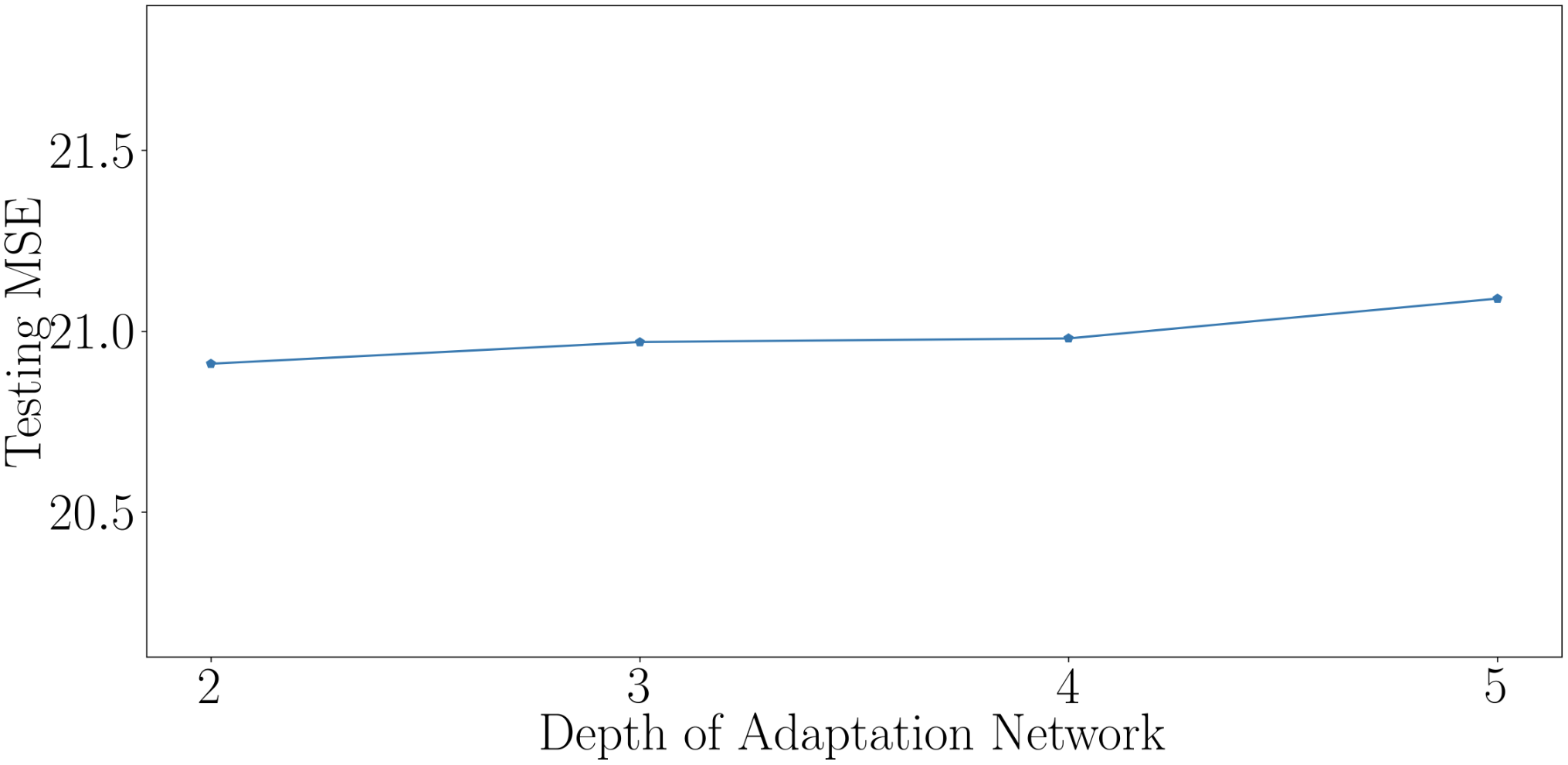
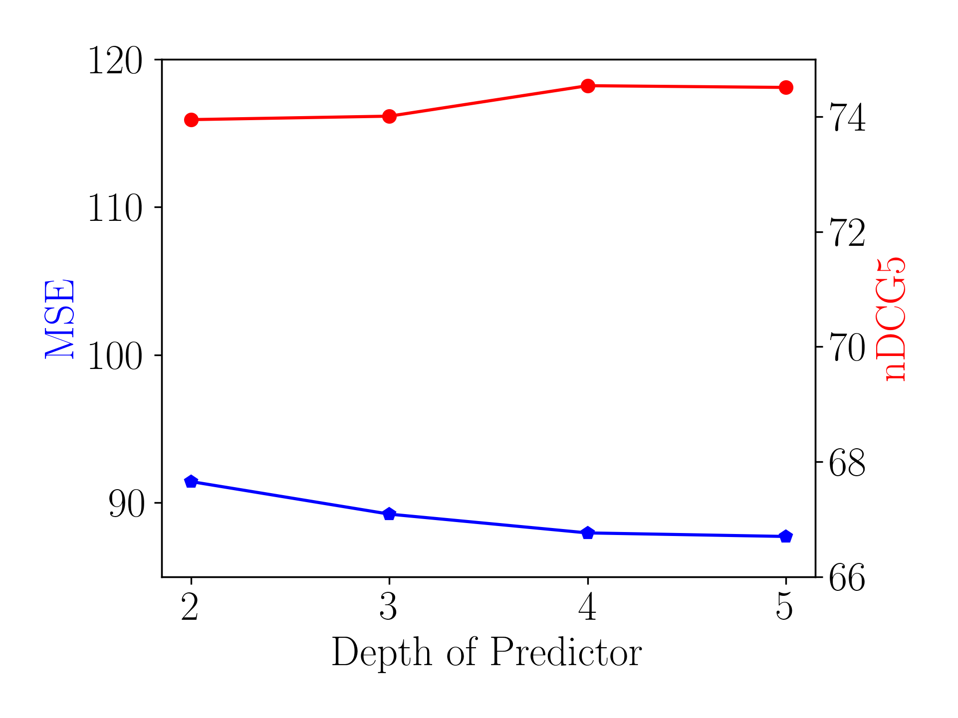
Here, we first show that the assumption of adaptation network being expressive enough can be easily satisfied. Generally, deeper networks are more expressive. Figure 6 plots the effect of changing the depth of the neural network in on Last.fm. As shown in Figure 6 (a-d), although different number of layers in are used, the searched modulation operations are the same. Consequently, the performance difference is small, as shown in Figure 6 (d). Thus, we use layers which is expressive enough and has smaller parameter size.
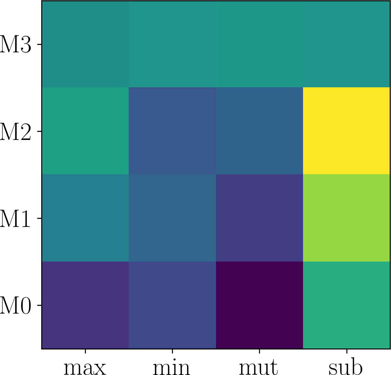
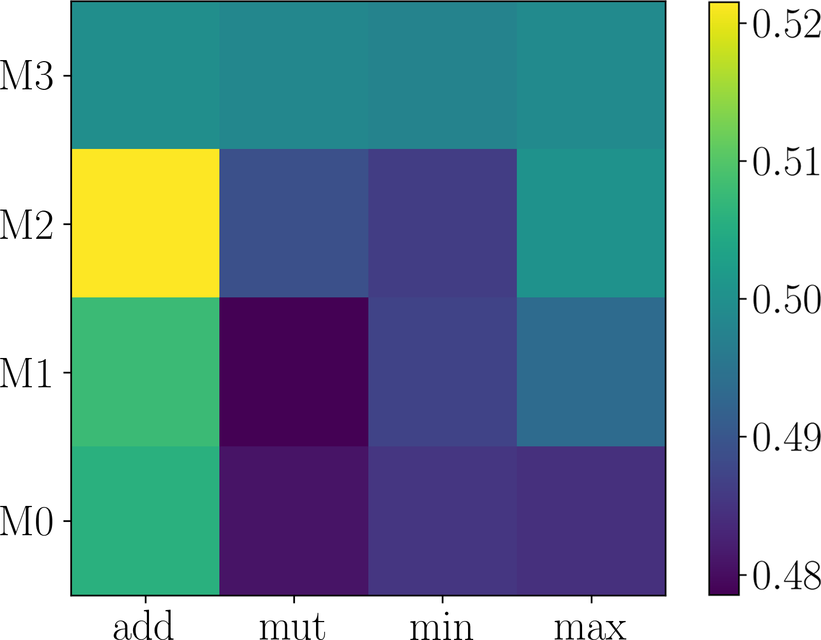
Further, we validate the inner-group consistence and permutation-invariance properties proved in Proposition 3.1. Comparing Figure 6 (a) with Figure 7 (a-b), one can see that changing to and to obtains the same results, which validates inner-group consistency. Finally, comparing Figure 6 (a) with Figure 7 (c), one can observe that inter-group permutation invariant also holds.

4.4. Sensitivity Analysis (RQ3)
Finally, we conduct sensitivity analysis of ColdNAS on Last.fm.
Effects of .
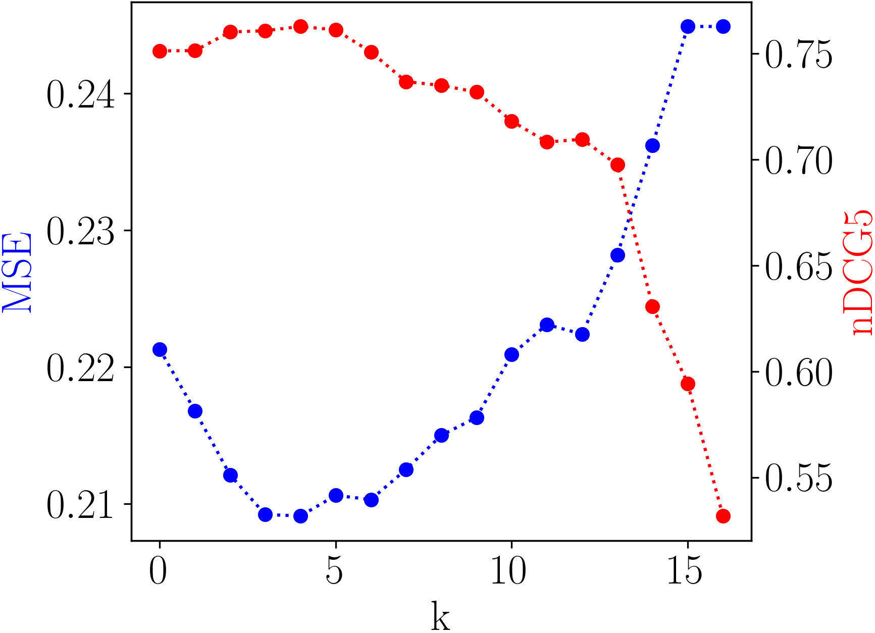
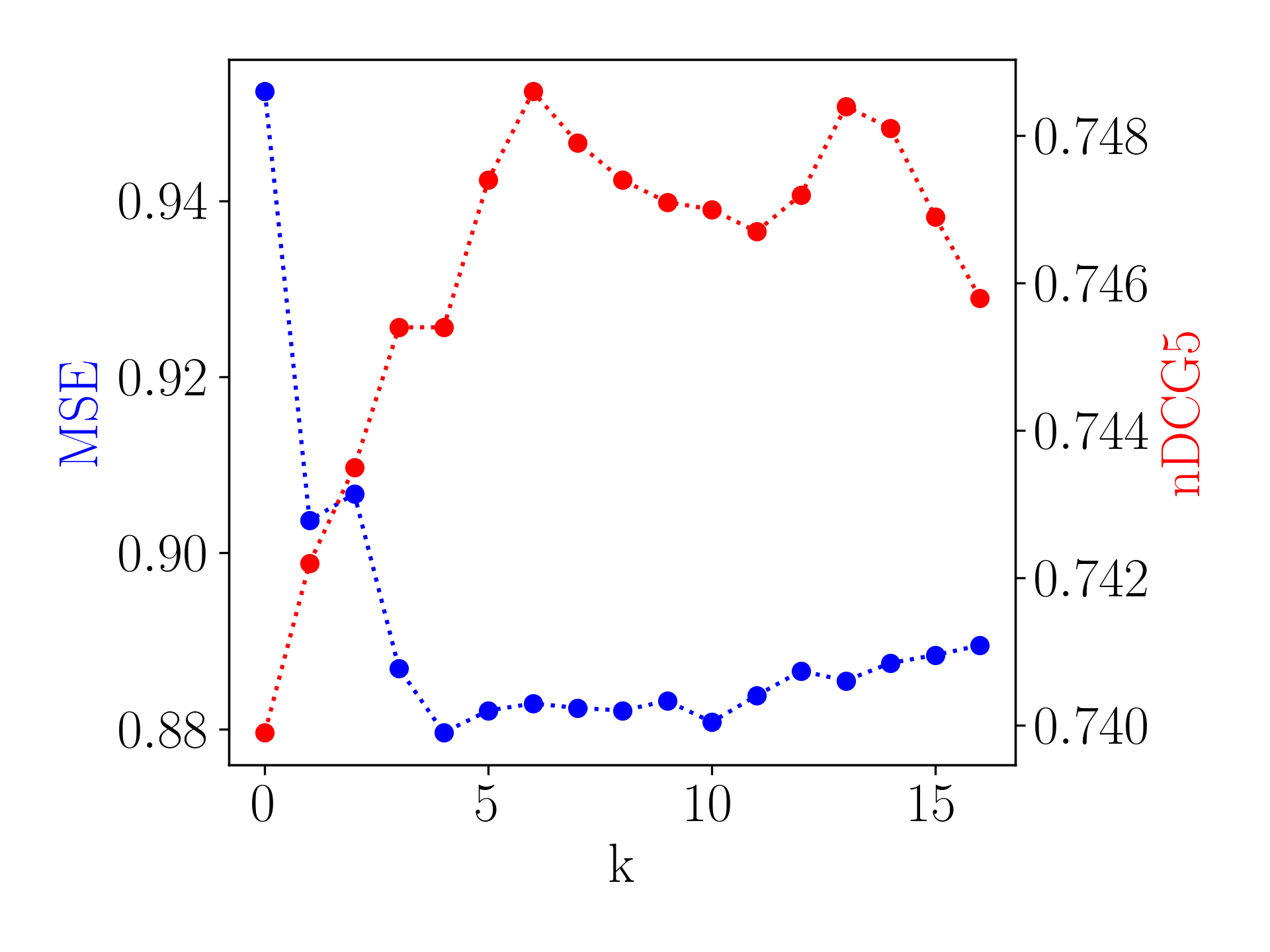
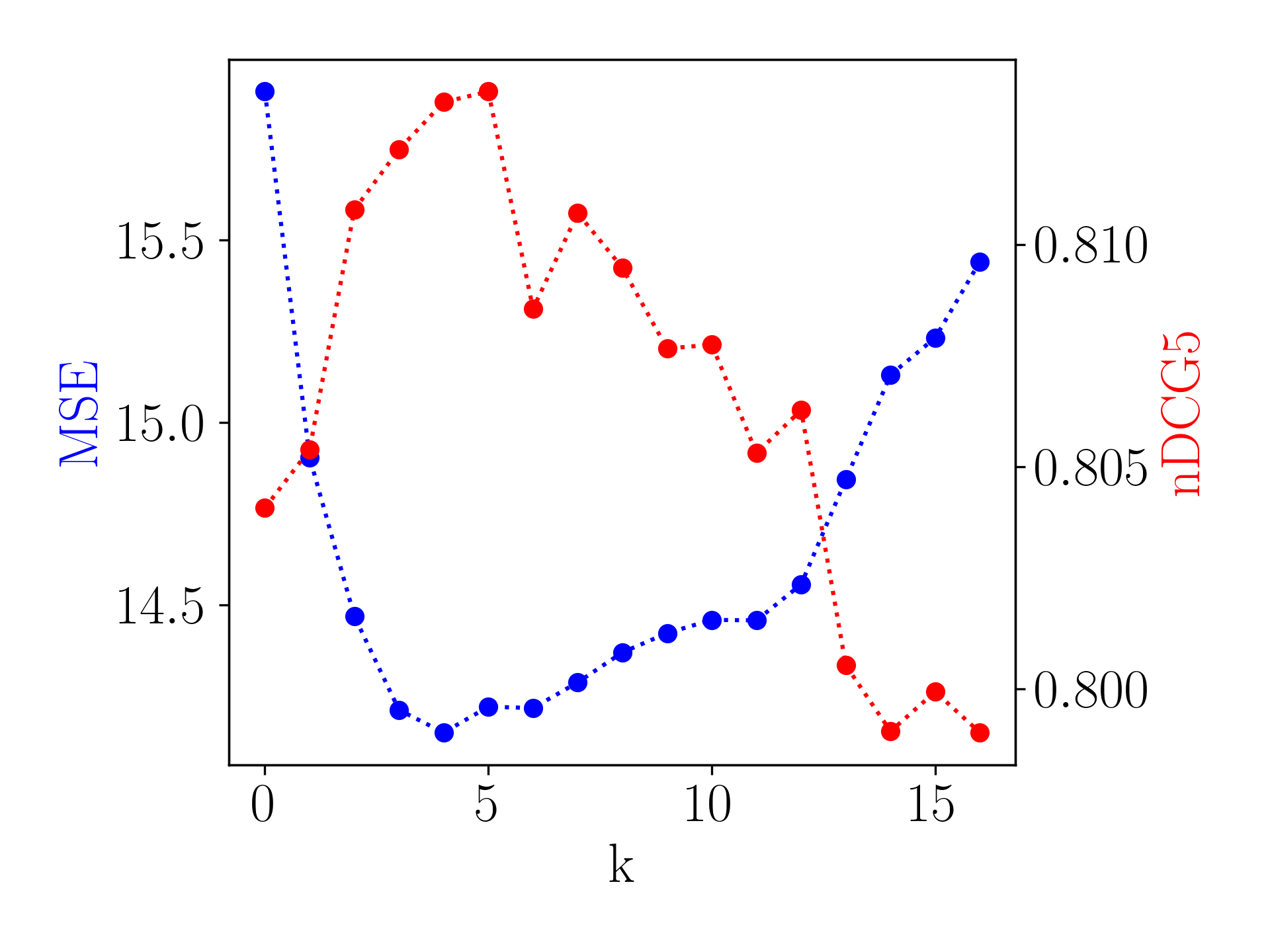
Recall that we keep modulation operations corresponding to the Top- largest s in modulation structure. Figure 5(a) plots the effect of changing . As shown, cannot be too small that the model is unable to capture enough user-specific preference, nor too large that the model can overfit to the limited interaction history of cold-start users.
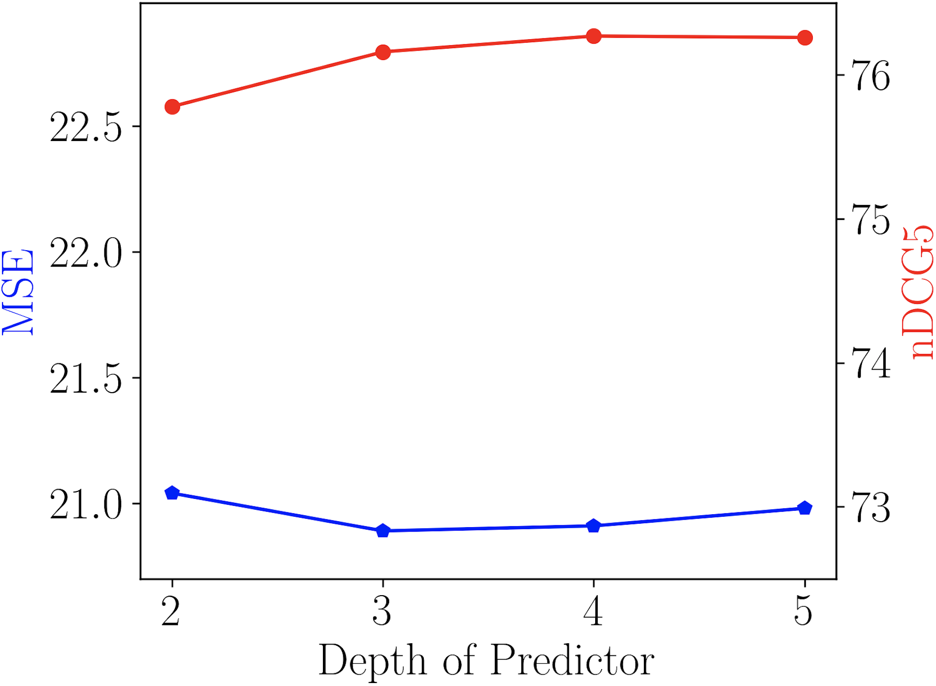
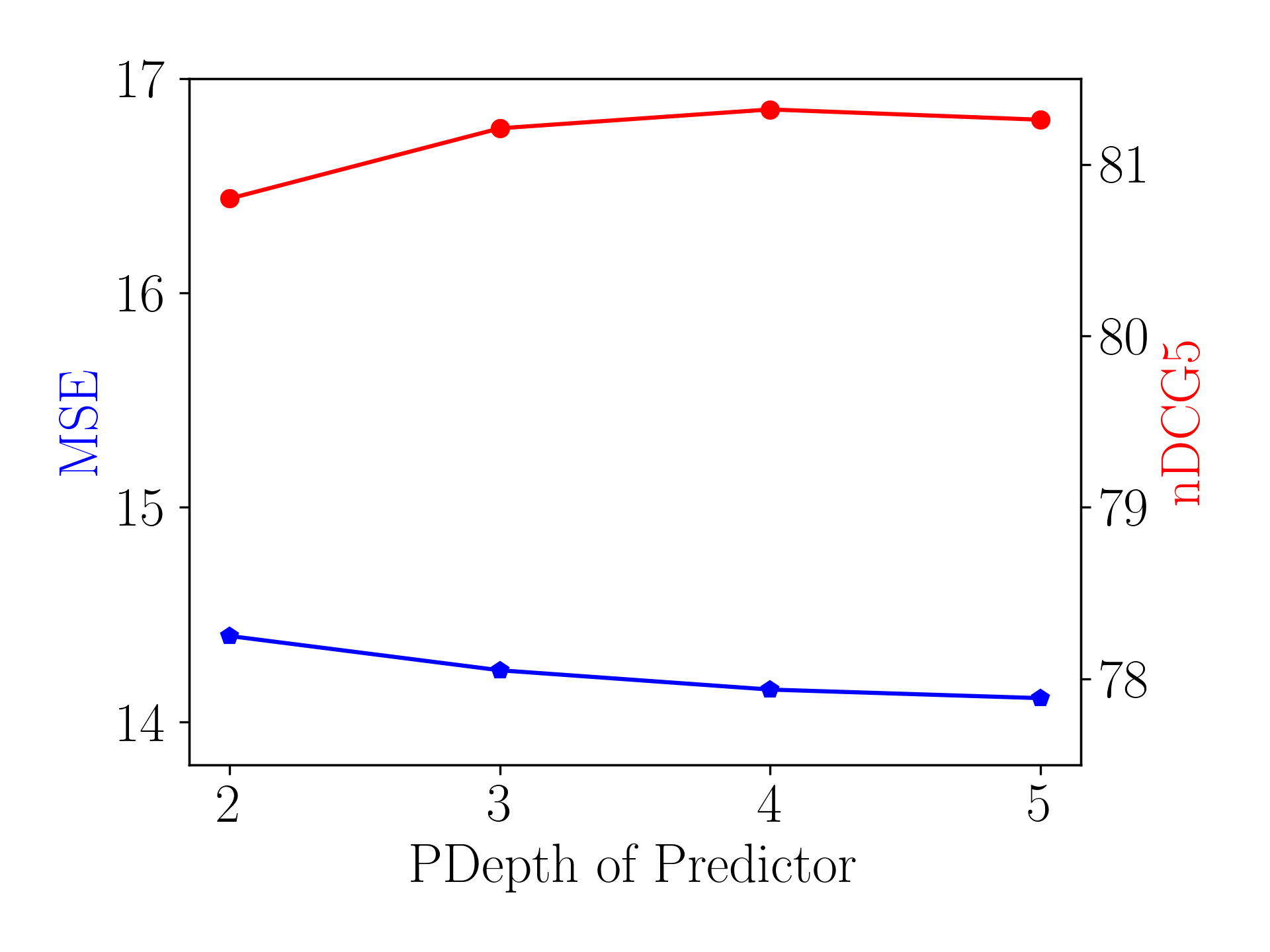
Effect of the Depth of Predictor.
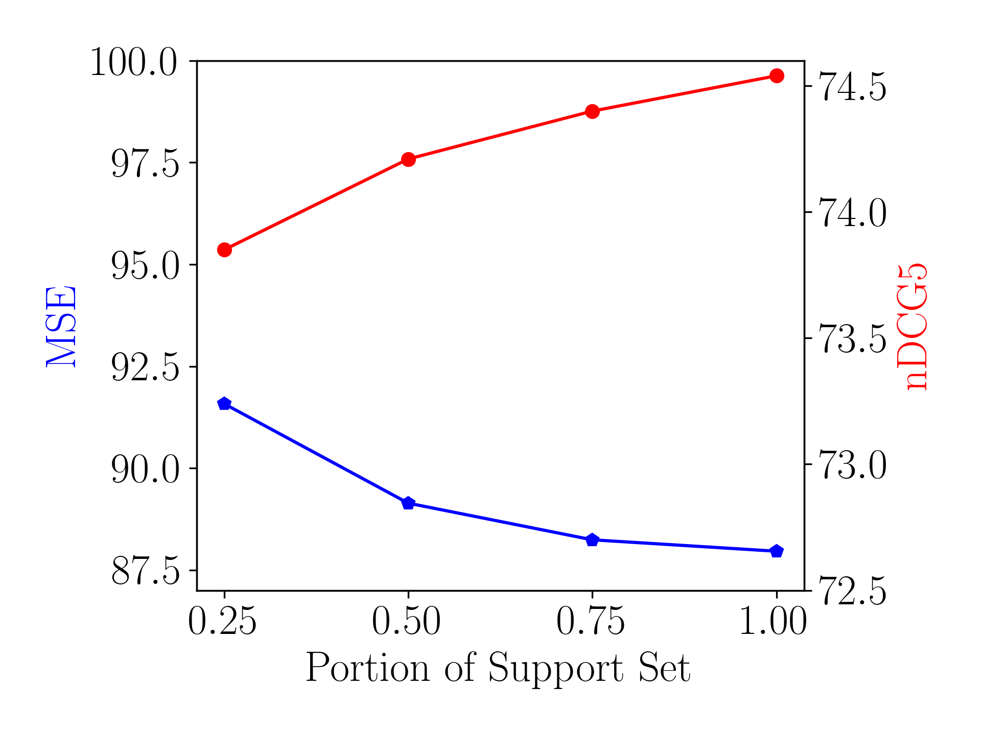
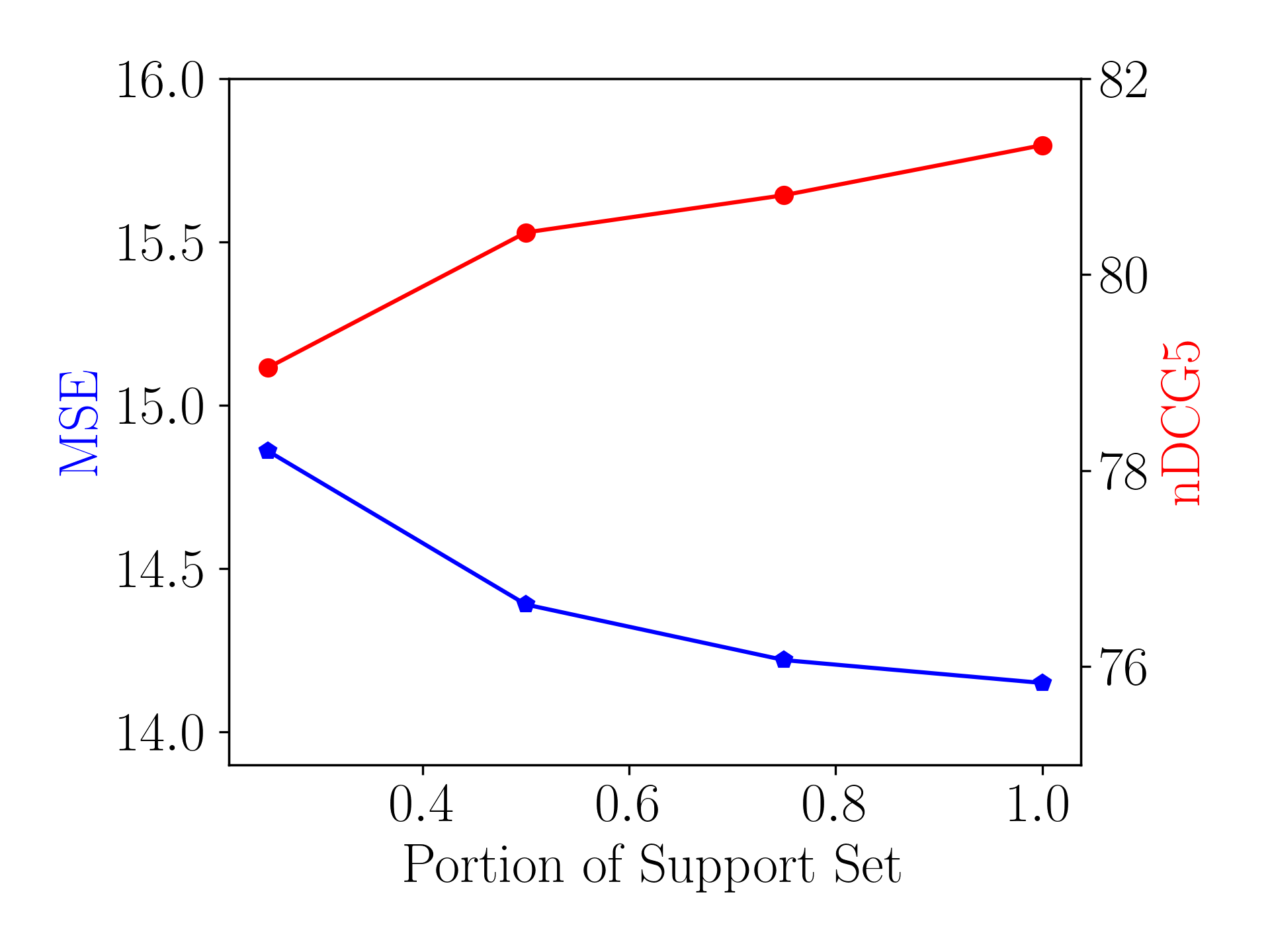
Effects of Support Set Size.
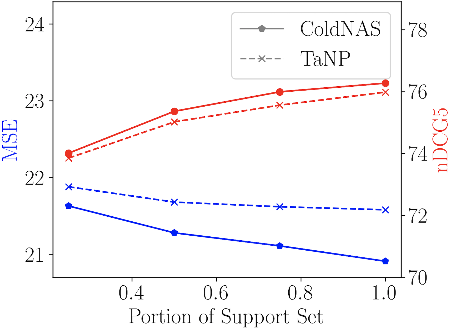
Figure 5(c) shows the performance of users with different length of history. During inference, we randomly sample only a portion of interactions from the original support set of each in . As can be seen, prediction would be more accurate given interaction history, which may alleviate the bias in representing the user-specific preference.
5. Conclusion
We propose a modulation framework called ColdNAS for user cold-start recommendation. In particular, we use a hypernetwork to map each user’s history interactions to user-specific parameters, which are then used to modulate the predictor. We design a search space for modulation functions and positions, which not only covers existing modulation-based models but also has the ability to find more effective structures. We theoretically prove the space could be transformed to a smaller space, where we can search for modulation structure efficiently and robustly. Extensive experiments show that ColdNAS performs the best on benchmark datasets. Besides, ColdNAS can efficiently find proper modulation structure for different data, which make it easy to be deployed in recommendation systems.
Acknowledgment
Q. Yao was in part supported by NSFC (No. 92270106) and CCF-Baidu Open Fund.
References
- (1)
- Baker et al. (2017) Bowen Baker, Otkrist Gupta, Nikhil Naik, and Ramesh Raskar. 2017. Designing neural network architectures using reinforcement learning. In International Conference on Learning Representations.
- Bergstra and Bengio (2012) James Bergstra and Yoshua Bengio. 2012. Random search for hyper-parameter optimization. Journal of Machine Learning Research 13, 2 (2012).
- Bharadhwaj (2019) Homanga Bharadhwaj. 2019. Meta-learning for user cold-start recommendation. In International Joint Conference on Neural Networks. 1–8.
- Brockschmidt (2020) Marc Brockschmidt. 2020. GNN-FiLM: Graph neural networks with feature-wise linear modulation. In International Conference on Machine Learning. 1144–1152.
- Cheng et al. (2016) Heng-Tze Cheng, Levent Koc, Jeremiah Harmsen, Tal Shaked, Tushar Chandra, Hrishi Aradhye, Glen Anderson, Greg Corrado, Wei Chai, Mustafa Ispir, et al. 2016. Wide & deep learning for recommender systems. In Workshop on Deep Learning for Recommender Systems. 7–10.
- Dong et al. (2020) Manqing Dong, Feng Yuan, Lina Yao, Xiwei Xu, and Liming Zhu. 2020. MAMO: Memory-augmented meta-optimization for cold-start recommendation. In ACM SIGKDD Conference on Knowledge Discovery and Data Mining. 688–697.
- Feng et al. (2021) Xidong Feng, Chen Chen, Dong Li, Mengchen Zhao, Jianye Hao, and Jun Wang. 2021. CMML: Contextual modulation meta learning for cold-start recommendation. In ACM International Conference on Information and Knowledge Management. 484–493.
- Finn et al. (2017) Chelsea Finn, Pieter Abbeel, and Sergey Levine. 2017. Model-agnostic meta-learning for fast adaptation of deep networks. In International Conference on Machine Learning. 1126–1135.
- Gao et al. (2021a) Chen Gao, Yinfeng Li, Quanming Yao, Depeng Jin, and Yong Li. 2021a. Progressive feature interaction search for deep sparse network. In Advances in Neural Information Processing Systems, Vol. 34. 392–403.
- Gao et al. (2021b) Chen Gao, Quanming Yao, Depeng Jin, and Yong Li. 2021b. Efficient Data-specific Model Search for Collaborative Filtering. In ACM SIGKDD Conference on Knowledge Discovery and Data Mining. 415–425.
- Ha et al. (2017) David Ha, Andrew Dai, and Quoc V Le. 2017. Hypernetworks. In International Conference on Learning Representations.
- Harper and Konstan (2015) F Maxwell Harper and Joseph A Konstan. 2015. The MovieLens datasets: History and context. ACM Transactions on Interactive Intelligent Systems 5, 4 (2015), 1–19.
- He et al. (2017) Xiangnan He, Lizi Liao, Hanwang Zhang, Liqiang Nie, Xia Hu, and Tat-Seng Chua. 2017. Neural collaborative filtering. In International Conference on World Wide Web. 173–182.
- Hornik et al. (1989) Kurt Hornik, Maxwell Stinchcombe, and Halbert White. 1989. Multilayer feedforward networks are universal approximators. Neural Networks 2, 5 (1989), 359–366.
- Hsieh et al. (2017) Cheng-Kang Hsieh, Longqi Yang, Yin Cui, Tsung-Yi Lin, Serge Belongie, and Deborah Estrin. 2017. Collaborative metric learning. In International Conference on World Wide Web. 193–201.
- Hutter et al. (2019) Frank Hutter, Lars Kotthoff, and Joaquin Vanschoren. 2019. Automated machine learning: methods, systems, challenges. Springer Nature.
- Jin et al. (2019) Haifeng Jin, Qingquan Song, and Xia Hu. 2019. Auto-Keras: An efficient neural architecture search system. In ACM SIGKDD Conference on Knowledge Discovery and Data Mining. 1946–1956.
- Koren (2008) Yehuda Koren. 2008. Factorization meets the neighborhood: A multifaceted collaborative filtering model. In ACM SIGKDD Conference on Knowledge Discovery and Data Mining. 426–434.
- Lee et al. (2019) Hoyeop Lee, Jinbae Im, Seongwon Jang, Hyunsouk Cho, and Sehee Chung. 2019. MeLU: Meta-learned user preference estimator for cold-start recommendation. In ACM SIGKDD Conference on Knowledge Discovery and Data Mining. 1073–1082.
- Lin et al. (2013) Jovian Lin, Kazunari Sugiyama, Min-Yen Kan, and Tat-Seng Chua. 2013. Addressing cold-start in app recommendation: latent user models constructed from twitter followers. In International ACM SIGIR Conference on Research and Development in Information Retrieval. 283–292.
- Lin et al. (2021) Xixun Lin, Jia Wu, Chuan Zhou, Shirui Pan, Yanan Cao, and Bin Wang. 2021. Task-adaptive neural process for user cold-start recommendation. In The Web Conference. 1306–1316.
- Liu et al. (2020) Bin Liu, Chenxu Zhu, Guilin Li, Weinan Zhang, Jincai Lai, Ruiming Tang, Xiuqiang He, Zhenguo Li, and Yong Yu. 2020. AutoFIS: Automatic feature interaction selection in factorization models for click-through rate prediction. In ACM SIGKDD Conference on Knowledge Discovery and Data Mining. 2636–2645.
- Liu et al. (2019) Hanxiao Liu, Karen Simonyan, and Yiming Yang. 2019. DARTS: Differentiable architecture search. In International Conference on Learning Representations.
- Lu et al. (2020) Yuanfu Lu, Yuan Fang, and Chuan Shi. 2020. Meta-learning on heterogeneous information networks for cold-start recommendation. In ACM SIGKDD Conference on Knowledge Discovery and Data Mining. 1563–1573.
- Luo et al. (2018) Renqian Luo, Fei Tian, Tao Qin, Enhong Chen, and Tie-Yan Liu. 2018. Neural architecture optimization. In Advances in Neural Information Processing Systems, Vol. 31. 7827–7838.
- Pang et al. (2022) Haoyu Pang, Fausto Giunchiglia, Ximing Li, Renchu Guan, and Xiaoyue Feng. 2022. PNMTA: A pretrained network modulation and task adaptation approach for user cold-start recommendation. In The Web Conference. 348–359.
- Park and Tuzhilin (2008) Yoon-Joo Park and Alexander Tuzhilin. 2008. The long tail of recommender systems and how to leverage it. In ACM Conference on Recommender Systems. 11–18.
- Perez et al. (2018) Ethan Perez, Florian Strub, Harm De Vries, Vincent Dumoulin, and Aaron Courville. 2018. FiLM: Visual reasoning with a general conditioning layer. In AAAI Conference on Artificial Intelligence, Vol. 32. 3942–3951.
- Pham et al. (2018) Hieu Pham, Melody Guan, Barret Zoph, Quoc Le, and Jeff Dean. 2018. Efficient neural architecture search via parameters sharing. In International Conference on Machine Learning. 4095–4104.
- Real et al. (2019) Esteban Real, Alok Aggarwal, Yanping Huang, and Quoc V Le. 2019. Regularized evolution for image classifier architecture search. In AAAI Conference on Artificial Intelligence, Vol. 33. 4780–4789.
- Requeima et al. (2019) James Requeima, Jonathan Gordon, John Bronskill, Sebastian Nowozin, and Richard E Turner. 2019. Fast and flexible multi-task classification using conditional neural adaptive processes. In Advances in Neural Information Processing Systems, Vol. 32. 7957–7968.
- Resnick and Varian (1997) Paul Resnick and Hal R Varian. 1997. Recommender systems. Commun. ACM 40, 3 (1997), 56–58.
- Schein et al. (2002) Andrew I Schein, Alexandrin Popescul, Lyle H Ungar, and David M Pennock. 2002. Methods and metrics for cold-start recommendations. In International ACM SIGIR Conference on Research and Development in Information Retrieval. 253–260.
- Sedhain et al. (2015) Suvash Sedhain, Aditya Krishna Menon, Scott Sanner, and Lexing Xie. 2015. AutoRec: Autoencoders meet collaborative filtering. In International Conference on World Wide Web. 111–112.
- Song et al. (2020) Qingquan Song, Dehua Cheng, Hanning Zhou, Jiyan Yang, Yuandong Tian, and Xia Hu. 2020. Towards automated neural interaction discovery for click-through rate prediction. In ACM SIGKDD Conference on Knowledge Discovery and Data Mining. 945–955.
- Volkovs et al. (2017) Maksims Volkovs, Guangwei Yu, and Tomi Poutanen. 2017. DropoutNet: Addressing cold start in recommender systems. In Advances in Neural Information Processing Systems, Vol. 30. 4957–4966.
- Wang et al. (2021) Li Wang, Binbin Jin, Zhenya Huang, Hongke Zhao, Defu Lian, Qi Liu, and Enhong Chen. 2021. Preference-adaptive meta-learning for cold-start recommendation.. In International Joint Conference on Artificial Intelligence. 1607–1614.
- Wang et al. (2020) Yaqing Wang, Quanming Yao, James T Kwok, and Lionel M Ni. 2020. Generalizing from a few examples: A survey on few-shot learning. Comput. Surveys 53, 3 (2020), 1–34.
- Xie et al. (2021) Yuexiang Xie, Zhen Wang, Yaliang Li, Bolin Ding, Nezihe Merve Gürel, Ce Zhang, Minlie Huang, Wei Lin, and Jingren Zhou. 2021. FIVES: Feature interaction via edge search for large-scale tabular data. In ACM SIGKDD Conference on Knowledge Discovery and Data Mining. 3795–3805.
- Yang et al. (2020) Yibo Yang, Hongyang Li, Shan You, Fei Wang, Chen Qian, and Zhouchen Lin. 2020. ISTA-NAS: Efficient and consistent neural architecture search by sparse coding. In Cross attention network for few-shot classification, Vol. 33. 10503–10513.
- Yao et al. (2020a) Quanming Yao, Xiangning Chen, James T Kwok, Yong Li, and Cho-Jui Hsieh. 2020a. Efficient neural interaction function search for collaborative filtering. In The Web Conference. 1660–1670.
- Yao et al. (2020b) Quanming Yao, Ju Xu, Wei-Wei Tu, and Zhanxing Zhu. 2020b. Efficient neural architecture search via proximal iterations. In AAAI Conference on Artificial Intelligence, Vol. 34. 6664–6671.
- Yu et al. (2019) Kaicheng Yu, Christian Sciuto, Martin Jaggi, Claudiu Musat, and Mathieu Salzmann. 2019. Evaluating the search phase of neural architecture search. In International Conference on Learning Representations.
- Yu et al. (2021) Runsheng Yu, Yu Gong, Xu He, Bo An, Yu Zhu, Qingwen Liu, and Wenwu Ou. 2021. Personalized adaptive meta learning for cold-start user preference prediction. In AAAI Conference on Artificial Intelligence, Vol. 35. 10772–10780.
- Zhang et al. (2023) Yongqi Zhang, Quanming Yao, and James T Kwok. 2023. Bilinear scoring function search for knowledge graph learning. IEEE Transactions on Pattern Analysis and Machine Intelligence 45, 2 (2023), 1458–1473.
- Zhao et al. (2021) Xiangyu Zhao, Haochen Liu, Wenqi Fan, Hui Liu, Jiliang Tang, and Chong Wang. 2021. AutoLoss: Automated loss function search in recommendations. In ACM SIGKDD Conference on Knowledge Discovery and Data Mining. 3959–3967.
- Ziegler et al. (2005) Cai-Nicolas Ziegler, Sean M McNee, Joseph A Konstan, and Georg Lausen. 2005. Improving recommendation lists through topic diversification. In International Conference on World Wide Web. 22–32.
Appendix A Details of Model Structure
As mentioned in Section 3.2, existing models (Dong et al., 2020; Lin et al., 2021; Pang et al., 2022) share an architecture consisting of three components: embedding layer , adaptation network , and predictor . Here we provide the details of these components used in ColdNAS.
A.1. Embedding Layer
We first embed user and item’s one-hot categorical features into dense vectors through the embedding layer. Taking for example, we generate a content embedding for each categorical content feature and concatenate them together to obtain the initial user embedding. Given user contents, the embedding is defined as:
| (11) |
where is the concatenation operation, is the one-hot vector of the th categorical content of , and represents the embedding matrix of the corresponding feature in the shared user feature space. The parameters of embedding layer are collectively denoted as .
A.2. Adaptation Network
We first use a fully connected (FC) layer to get hidden representation of interaction history , which is calculated as
| (12) |
We use mean pooling to aggregate the interactions in as the task context information of , i.e.,preference, . Then, we use another FC layer to generate the user-specific parameters as . The parameters of adaptation network is denoted as .
A.3. Predictor
We use a -layer MLP as the predictor. Denote output of the th layer hidden units as , the modulation function at the th layer as , we obtain prediction by
| (13) |
where , and . The parameters of predictor are denoted as .
Appendix B Proof of the Proposition 3.1
Proof.
To prove Proposition 3.1, we need to use the two conditions below:
Condition 1: If is the input of operation or , then every element in is non-negative. We implement this as ReLU function.
Condition 2: The adaptation network is expressive enough, that it can approximate , where and , learned from the data. This naturally holds due to the assumption.
Divide into 4 groups: . We can prove two important properties below.
Property 1: Inner-group consistence
.We can choose an operation in each group as the group operation , e.g. . Then any number of successive operations that belong to the same group can be associated into one operation , i.e.,
It’s trivial to prove with condition 2, e.g., , where .
Property 2: Inter-group permutation-invariance.
The operations in different groups are permutation-invariant, i.e.,
It is also trivial to prove with condition 1 and condition 2, e.g.,
where and .
With the above two properties, we can recurrently commute operations until operations in the same group are gathered, and merge operations in the four groups respectively. So
equals to
and the four group operations are permutation-invariant.
Note that since the identity element (0 or 1) of each group operation can be learned from condition 2, a modulation function that doesn’t cover all groups can also be represented in the same form. ∎
Appendix C Experiments
C.1. Experiment Setting
Experiments were conducted on a 24GB NVIDIA GeForce RTX 3090 GPU, with Python 3.7.0, CUDA version 11.6.
C.1.1. Hyperparameter Setting
We find hyperparameters using the via grid search for existing methods. In ColdNAS, the batch size is 32, in (11) has size where is the length of . The dimension of hidden units in (13) is set as for all three datasets. The learning rate is chosen from and the dimension of in (12) is chosen from . The final hyperparameters chosen on the three benchmark datasets are shown in Table 6.
| Dataset | MovieLens | BookCrossing | Last.fm |
|---|---|---|---|
| 1024 | 512 | 256 | |
| 128 | |||
| 64 | |||
| 32 | 32 | ||
| 1 | 1 | 1 | |
| maximum iteration number | 50 | 50 | 100 |
C.1.2. URLs of Datasets and Baselines
We use three benchmark datasets (Table 4): (i) MovieLens222https://grouplens.org/datasets/movielens/1m/ (Harper and Konstan, 2015): a dataset containing 1 million movie ratings of users collected from MovieLens, whose features include gender, age, occupation, Zip code, publication year, rate, genre, director and actor; (ii) BookCrossing333http://www2.informatik.uni-freiburg.de/~cziegler/BX/ (Ziegler et al., 2005): a collection of users’ ratings on books in BookCrossing community, whose features include age, location, publish year, author, and publisher; and (iii) Last.fm444https://grouplens.org/datasets/hetrec-2011/: a collection of user’s listening count of artists from Last.fm online system, whose features only consist of user and item IDs. In experiments, we compare ColdNAS with the following representative user cold-start methods: (i) traditional deep cold-start model DropoutNet555https://github.com/layer6ai-labs/DropoutNet (Volkovs et al., 2017) and (ii) FSL based methods include MeLU666https://github.com/hoyeoplee/MeLU (Lee et al., 2019), MetaCS (Bharadhwaj, 2019), MetaHIN777https://github.com/rootlu/MetaHIN (Lu et al., 2020), MAMO888https://github.com/dongmanqing/Code-for-MAMO (Dong et al., 2020), and TaNP999https://github.com/IIEdm/TaNP (Lin et al., 2021). MetaCS is very similar to MeLU, except that it updates all parameters during meta-learning. Hence, we implement MetaCS based on the codes of MeLU.
C.2. More Experimental Results
C.3. Complexity Analysis
Denote the layer number of adaptation network as , the layer number of predictor as , the support set size as , and the query set size as . For notation simplicity, we denote the hidden size of each layer is the same as . In the search phase (Algorithm 1 step 210), the calculation of of a task is , and predicting each item costs , so the average complexity is . Similarly, in the retrain (Algorithm 1 step 1213), the time complexity is also . In total, the time complexity is .