BatchSampler: Sampling Mini-Batches for Contrastive Learning in Vision, Language, and Graphs

Abstract.

In-Batch contrastive learning is a state-of-the-art self-supervised method that brings semantically-similar instances close while pushing dissimilar instances apart within a mini-batch. Its key to success is the negative sharing strategy, in which every instance serves as a negative for the others within the mini-batch. Recent studies aim to improve performance by sampling hard negatives within the current mini-batch, whose quality is bounded by the mini-batch itself. In this work, we propose to improve contrastive learning by sampling mini-batches from the input data. We present BatchSampler to sample mini-batches of hard-to-distinguish (i.e., hard and true negatives to each other) instances. To make each mini-batch have fewer false negatives, we design the proximity graph of randomly-selected instances. To form the mini-batch, we leverage random walk with restart on the proximity graph to help sample hard-to-distinguish instances. BatchSampler is a simple and general technique that can be directly plugged into existing contrastive learning models in vision, language, and graphs. Extensive experiments on datasets of three modalities show that BatchSampler can consistently improve the performance of powerful contrastive models, as shown by significant improvements of SimCLR on ImageNet-100, SimCSE on STS (language), and GraphCL and MVGRL on graph datasets.

1. Introduction

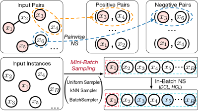
Figure 1. Technical comparison between Mini-Batch Sampling, Pairwise Negative Sampling (NS), and In-Batch Negative Sampling. The blue nodes are hard negatives.

Contrastive learning (Oord et al., 2018; Jaiswal et al., 2020) is one of the dominant strategies for self-supervised representation learning across various data domains, such as MoCo (He et al., 2020) and SimCLR (Chen et al., 2020) in computer vision, SimCSE (Gao et al., 2021) in natural language processing, and GraphCL (You et al., 2020) in graph representation learning. The essence of self-supervised contrastive learning is to make similar instances close to each other and dissimilar ones farther away in the learned representation space.

The course of self-supervised contrastive models usually starts with loading each mini-batch of $B$ instances sequentially from the input data (e.g., the images in Figure 2 (a)). In each batch, each instance $x$ is associated with its augmentation $x^{+}$ as the positive samples and the other instances as negatives $\{x^{-}\}$. Commonly by using the InfoNCE loss (Oord et al., 2018), the goal of contrastive learning is to discriminate instances by mapping positive pairs ($x,x^{+}$) to similar embeddings and negative pairs ($x,x^{-}$) to dissimilar embeddings.

Given the self-supervised contrastive setting, the negative samples $\{x^{-}\}$—with unknown labels—play an essential role in the contrastive optimization process. To improve in-batch contrastive learning, there are various attempts to take on them from different perspectives. Globally, SimCLR (Chen et al., 2020) shows that simply increasing the size $B$ of the mini-batch (e.g., 8192)—i.e., more negative samples—outperforms previously carefully-designed strategies, such as the memory bank (Wu et al., 2018) and the consistency improvement of the stored negatives in MoCo (He et al., 2020). Locally, given each mini-batch, recent studies such as the DCL and HCL (Robinson et al., 2021; Chuang et al., 2020) methods have focused on identifying true or hard negatives within this batch. In other words, existing efforts have largely focused on designing better negative sampling techniques after each mini-batch of instances is loaded.

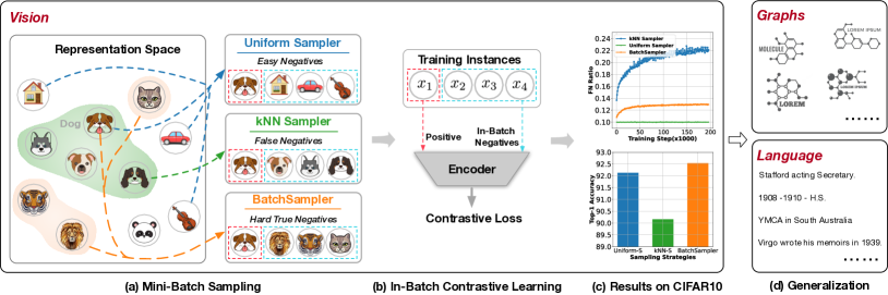
Figure 2. A motivating illustration of BatchSampler, using vision as an example. Uniform Sampler randomly samples a batch of instances, which contains easy negatives. kNN Sampler selects the nearest instances to form a batch, resulting in so many false negatives. BatchSampler samples a mini-batch with hard yet true negatives based on proximity graph.

Problem. In this work, we instead propose to globally sample instances from the input data to form mini-batches. The goal is to have mini-batches that naturally contain as many hard negatives $\{x^{-}\}$—that have different (underlying) labels from $x$ (true negatives) but similar representations with $x$—for each instance $x$ as possible. In this way, the discrimination between positive and negative instances in each mini-batch can better inform contrastive optimization.

Uniform & kNN Samplers. Traditionally, there are two ways to form mini-batches (Cf. Figure  2 (a)). The common option is the Uniform Sampler that sequentially loads or uniformly samples a batch of instances for each training step(Chen et al., 2020; Gao et al., 2021; You et al., 2020). However, the Uniform Sampler neglects the effect of hard negatives (Kalantidis et al., 2020; Robinson et al., 2021), and the batches formed contain easy negatives with low gradients that contribute little to optimization (Yang et al., 2020; Xiong et al., 2020). In order to have hard negatives, it is natural to cluster instances that are nearest to each other in the representation space to form each batch, that is, the kNN Sampler. Unfortunately, the instances with the same underlying labels are also expected to cluster together (Chen et al., 2020; Caron et al., 2020), resulting in high percentages of false negatives in the batch (Cf. Figure  2 (c)).

Contributions: BatchSampler. We present BatchSampler to sample mini-batches of hard-to-distinguish instances for in-batch contrastive learning. Fundamentally, each mini-batch is required to cover hard yet true negatives, thus addressing the issues faced by Uniform and kNN Samplers. To achieve this, we design the proximity graph of randomly-selected instances in which each edge is used to control the pairwise similarity of their representations—that is, the hardness of negative samples. The false negative issue in the kNN Sampler is mitigated when random instances are picked to construct the graph. To form one batch, we leverage random walk with restart on the proximity graph to draw instances. The premise is that the local neighbors sampled by the walkers are similar, that is, hard-to-distinguish.

BatchSampler is a simple and general technique that can be directly plugged into in-batch contrastive models in vision, language, and graphs. The experimental results show that the well-known contrastive learning models—SimCLR (Chen et al., 2020) and MoCo v3 (Chen et al., 2021) in vision, SimCSE (Gao et al., 2021) in language, and GraphCL (You et al., 2020) and MVGRL (Hassani and Khasahmadi, 2020) in graphs—can benefit from the mini-batches formed by BatchSampler. We also theoretically and empirically show that how BatchSampler balances the challenges faced in the Uniform and kNN Samplers.

Differences from Pairwise Negative Sampling. The problem of mini-batch sampling is different from the pairwise negative sampling problem. As shown in Figure 1, the pairwise negative sampling method samples negative instances for each positive pair, whereas the mini-batch sampling methods focus on sampling mini-batches that reuses other instances as negatives in the batch. Massive previous works in pairwise negative sampling (Huang et al., 2020; Xiong et al., 2020; Karpukhin et al., 2020; Yang et al., 2020; Huang et al., 2021) have attempted to improve performance by globally selecting similar negatives for a given anchor from the entire dataset. However, our focus is on globally sampling mini-batches that contain many hard negatives rather than only selecting hard negatives for each pair.

2. Related Work

Contrastive learning in different modalities. Contrastive learning follows a similar paradigm that contrasts similar and dissimilar observations based on noise contrastive estimation (NCE) (Gutmann and Hyvärinen, 2010; Oord et al., 2018). The primary distinction between contrastive methods of different modalities is how they augment the data. As for computer vision, MoCo (He et al., 2020) and SimCLR (Chen et al., 2020) augment data with geometric transformation and appearance transformation. Besides simply using data augmentation, WCL (Zheng et al., 2021) additionally utilizes an affinity graph to construct positive pairs for each example within the mini-batch. Wu et al. (2021) design a data replacement strategy to mine hard positive instances for contrastive learning. As for language, CLEAR (Wu et al., 2020b) and COCO-LM (Meng et al., 2021) augment the text data through word deletion, reordering, and substitution, while SimCSE (Gao et al., 2021) obtains the augmented instances by applying the standard dropout twice. As for graphs, DGI (Petar et al., 2018) and InfoGraph (Sun et al., 2019) treat the node representations and corresponding graph representations as positive pairs. Besides, InfoGCL(Xu et al., 2021), JOAO (You et al., 2021), GCA (Zhu et al., 2021b), GCC (Qiu et al., 2020) and GraphCL (You et al., 2020) augment the graph data by graph sampling or proximity-oriented methods. MVGRL (Hassani and Khasahmadi, 2020) proposes to compare the node representation in one view with the graph representation in the other view. Zhu et al. (2021a) compares different kinds of graph augmentation strategies. Our proposed BatchSampler is a general mini-batch sampler that can directly be applied to any in-batch contrastive learning framework with different modalities.

Negative sampling in contrastive learning. Previous studies about negative sampling in contrastive learning roughly fall into two categories: (1) Memory-based negative sampling strategy, such as MoCo (He et al., 2020), maintains a fixed-size memory bank to store negatives which are updated regularly during the training process. MoCHI (Kalantidis et al., 2020) and m-mix (Zhang et al., 2022) propose to mix the hard negative candidates at the feature level to generate more challenging negative pairs. MoCoRing (Wu et al., 2020a) samples hard negatives from a defined conditional distribution which keeps a lower bound on the mutual information. (2) In-batch negative sharing strategy, such as SimCLR (Chen et al., 2020) and MoCo v3 (Chen et al., 2021), adopts different instances in the current mini-batch as negatives. To mitigate the false negative issue, DCL (Chuang et al., 2020) modifies the original InfoNCE objective to reweight the contrastive loss. Huynh et al. (2022) identifies the false negatives within a mini-batch by comparing the similarity between negatives and the anchor image’s multiple support views. Additionally, HCL (Robinson et al., 2021) revises the original InfoNCE objective by assigning higher weights for hard negatives among the mini-batch. Recently, UnReMix (Tabassum et al., 2022) is proposed to sample hard negatives by effectively capturing aspects of anchor similarity, representativeness, and model uncertainty. However, such locally sampled hard negatives cannot exploit hard negatives sufficiently from the dataset.

Global hard negative sampling methods on triplet loss have been widely investigated, which aim to globally sample hard negatives for a given positive pair. For example, Wang et al. (2021) proposes to take rank-k hard negatives from some randomly sampled negatives. Xiong et al. (2020) globally samples hard negatives by an asynchronously-updated approximate nearest neighbor (ANN) index for dense text retrieval. Different from the above methods which are applied to a triplet loss for a given pair, BatchSampler samples mini-batches with hard negatives for InfoNCE loss.

3. Problem: Mini-Batch Sampling for Contrastive Learning

In-Batch Contrastive Learning. In-batch contrastive learning commonly follows or slightly updates the following objective (Gutmann and Hyvärinen, 2010; Oord et al., 2018) across different domains, such as graphs (You et al., 2020; Qiu et al., 2020), vision (Chen et al., 2020; Chen et al., 2021), and language (Gao et al., 2021):

(1) $$\text{min}\ \ \mathbb{E}_{\{x_{1}...\ x_{B}\}\subset\mathcal{D}}\left[-\sum_{i=1}^{B}\log\frac{e^{f(x_{i})^{T}f(x_{i}^{+})}}{e^{f(x_{i})^{T}f(x_{i}^{+})}+\sum_{j\neq i}e^{f(x_{i})^{T}f(x_{j})}}\right],$$

where $\{x_{1}...\ x_{B}\}$ is a mini-batch of samples (usually) sequentially loaded from the dataset $\mathcal{D}$, and $x_{i}^{+}$ is an augmented version of $x_{i}$. The encoder $f(\cdot)$ learns to discriminate instances by mapping different data-augmentation versions of the same instance (positive pairs) to similar embeddings, and mapping different instances in the mini-batch (negative pairs) to dissimilar embeddings.

Usually, the in-batch negative sharing strategy—every instance serves as a negative to the other instances within the mini-batch—is used to boost the training efficiency (Chen et al., 2020). It is then natural to have hard negatives in each mini-batch for improving contrastive learning. Straightforwardly, we could attempt to sample hard negatives within the mini-batch (Chuang et al., 2020; Robinson et al., 2021; Karpukhin et al., 2020). However, the batch size of a mini-batch is—by definition—far smaller than the size of the input dataset, and existing studies show that sampling such a local sampling method fails to effectively explore all the hard negatives (Xiong et al., 2020; Zhang et al., 2013).

Problem: Mini-Batch Sampling. The goal of this work is to have a general mini-batch sampling strategy to support different modalities of data. Specifically, given a set of data instances $\mathcal{D}=\{x_{1},\cdots,x_{N}\}$, the objective is to design a modality-independent sampler to sample a mini-batch of instances where each pair of instances are hard to distinguish across the dataset.

There are two existing strategies—Uniform Sampler and kNN Sampler—adopted in contrastive learning.

Uniform Sampler is the most common strategy used in contrastive learning (Chen et al., 2020; Gao et al., 2021; You et al., 2020). The pipeline is to first randomly sample a batch of instances for each training step, then feed them into the model for optimization.

Though simple and model-independent, Uniform Sampler neglects the effect of hard negatives (Kalantidis et al., 2020; Robinson et al., 2021), and the batches formed contain negatives with low gradients that contribute little to optimization. Empirically, we show that Uniform Sampler results in a low percentage of similar instance pairs in a mini-batch (Cf. Figure 4). Theoretically, Yang et al. (2020) and Xiong et al. (2020) also prove that the sampled negative should be similar to the query instance since it can provide a meaningful gradient to the model.

kNN Sampler globally samples a mini-batch with many hard negatives. As its name indicates, it tries to pick an instance at random and retrieve a set of nearest neighbors to construct a batch.

However, the instances of the same ‘class’ will be clustered together in the embedding space  (Chen et al., 2020; Caron et al., 2020). Hence the negatives retrieved by it are hard at first but would be replaced by false negatives (FNs) as the training epochs increase, misguiding the model training.

In summary, Uniform Sampler leverages random negatives to guide the optimization of the model; whereas the kNN one explicitly samples hard negatives but suffers from false negatives. Thus, an ideal negative sampler for in-batch contrastive learning should balance between kNN and Uniform Samplers, ensuring both the exploitation of hard negatives and the mitigation of the FN issue.

4. The BatchSampler Method

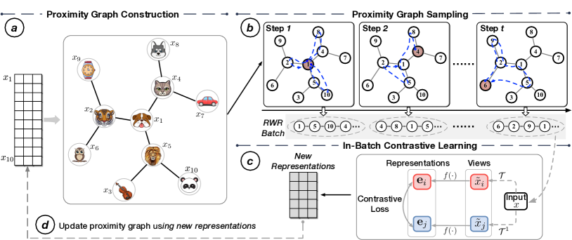
Figure 3. The framework of BatchSampler, using the vision modality as an example. The proximity graph is first constructed based on generated image representations and will be updated every $t$ training step. Next, a proximity graph-based negative sampler is applied to generate a batch with hard negatives for in-batch contrastive learning.

To improve contrastive learning, we propose the BatchSampler method with the goal of forming mini-batches with 1) hard-to-distinguish instances while 2) avoiding false negatives. BatchSampler is a simple and general strategy that can be directly plugged into existing in-batch contrastive learning models in vision, language, and graphs. Figure  3 shows the overview of BatchSampler.

The basic idea of BatchSampler is to form mini-batches by globally sampling instances based on the similarity between each pair of them, which is significantly different from previous local sampling methods in contrastive learning (Chuang et al., 2020; Robinson et al., 2021; Kalantidis et al., 2020). To achieve this, the first step of BatchSampler is to construct the proximity graph of instances with edges measuring the pairwise similarity. Second, we perform mini-batch sampling as a walk by leveraging a simple and commonly-used graph sampling technique, random walk with restart, to sample instances (nodes) from the proximity graph.

4.1. Proximity Graph Construction

The goal of the proximity graph is to collect candidate instances that alleviate the issues faced by Uniform and kNN Sampler by connecting similar instances while reducing the false negative pairs. If neighbors of an instance are randomly chosen from the dataset, sampling on the resulting graph resembles Uniform Sampler. Conversely, if the most similar instances are chosen as neighbors, it resembles the behavior of kNN Sampler. In BatchSampler, we propose a simple strategy to construct the proximity graph as follows.

Given a training dataset, we have $N$ instances $\{v_{i}|i=1,\cdots,N\}$ and their corresponding representations $\{\mathbf{e}_{i}|i=1,\cdots,N\}$ generated by the encoder $f(\cdot)$. The proximity graph is formulated as:

(2) $$G=(\mathcal{V},\mathcal{E}),$$

where the node set $\mathcal{V}=\{v_{1},\cdots,v_{N}\}$ denotes the instances and $\mathcal{E}\subseteq\{(v_{i},v_{j})|v_{i},v_{j}\in\mathcal{V}\}$ is a set of node pairs. Let $\mathcal{N}_{i}$ be the neighbor set of $v_{i}$ in the proximity graph. To construct $\mathcal{N}_{i}$, we first form a candidate set $\mathcal{C}_{i}=\{v_{m}\}$ for each instance $v_{i}$ by uniformly picking $M(M\ll N)$ neighbor candidates. Each node and its neighbor form an edge, resulting in the edge set $\mathcal{E}$. Then we select the $K$ nearest ones from the candidate set:

(3) $$\mathcal{N}_{i}=\mathop{\text{TopK}}\limits_{v_{m}\in\mathcal{C}_{i}}\left(\mathbf{e}_{i}\cdot\mathbf{e}_{m}\right),$$

where $\cdot$ is the inner product operation. $M$ is used to control the similarity between the center node and its immediate neighbor nodes, which can be demonstrated by the following proposition:

Proposition 1.

Given an instance $v_{i}$ with the corresponding representation $\mathbf{e}_{i}$, assume that there are at least $S$ instances whose inner product similarity with $v_{i}$ is larger than $s$, i.e.,

(4) $$\left|\left\{v_{j}\in\mathcal{V}\mid\mathbf{e}_{i}\cdot\mathbf{e}_{j}>s\right\}\right|\geq S.$$

Then in the proximity graph $G$, the similarity between $v_{i}$ and its neighbors is larger than $s$ with proximate probability at least:

(5) $$\mathbb{P}\left\{\mathbf{e}_{i}\cdot\mathbf{e}_{k}>s,\forall v_{k}\in\mathcal{N}_{i}\right\}\gtrapprox\left(1-p^{M}\right)^{K},$$

where $p=\frac{N-S}{N}$, and $K$ is the number of neighbors.

Proof.

Since $M\ll N$, we can approximately assume that the sampling is with replacement. In this case, we have

(6) $$\mathbb{P}\left\{\mathbf{e}_{i}\cdot\mathbf{e}_{k}>s,\forall v_{k}\in\mathcal{N}_{i}\right\}=1-\sum_{k=0}^{K-1}{M\choose k}p^{M-k}\left(1-p\right)^{k}.$$

Then let us prove (5) by induction. When $K=1$, the conclusion clearly holds.

Assuming that the conclusion holds when $K=L-1$, let us consider the case when $K=L$. We have

(7) $$1-\sum_{k=0}^{L-1}{M\choose k}p^{M-k}(1-p)^{k}\gtrapprox\left(1-p^{M}\right)^{L-1}-{M\choose L-1}p^{M-L+1}\left(1-p\right)^{L-1}.$$

To prove the conclusion, we only need to show

(8) $$\left(1-p^{M}\right)^{L-1}p^{M}\gtrapprox{M\choose L-1}p^{M-L+1}\left(1-p\right)^{L-1},$$

or equivalently

(9) $$\left(1-p^{M}\right)^{L-1}p^{L-1} =\left(1-p^{M}\right)^{L-1}\left(\frac{N-S}{N}\right)^{L-1}$$

$$\gtrapprox{M\choose L-1}\left(\frac{S}{N}\right)^{L-1}={M\choose L-1}\left(1-p\right)^{L-1}.$$

On the other hand, according to (Knuth, 1997), we have

(10) $${M\choose L-1}\leq\left(\frac{eM}{L-1}\right)^{L-1},$$

where $e$ denotes the Euler’s number. Substituting (10) into (9), we only need to show

(11) $$(N-S)(L-1)\left(1-p^{M}\right)\gtrapprox eMS.$$

The above relation holds depending on the choices of $M$, $S$ and $L$, which can be satisfied in our scenario in most cases. ∎

Proposition 1 suggests that the candidate set size $M$ can control the similarity between each center node and its immediate neighbor nodes. A larger $M$ indicates a greater probability that two adjacent nodes are similar, and the proximity graph constructed would be more like the graph of nodes clustered by kNN. If $M$ is small and close to $K$, the instances in the proximity graph can be considered as randomly-selected ones, that is, by Uniform Sampler.

4.2. Proximity Graph Sampling

We perform the mini-batch sampling as a walk in the proximity graph, which collects the visited instances as sampling results from a sourced node. Here we propose to apply Random Walk with Restart (RWR), which offers a theoretically supported ability to control the walker’s behavior.

As shown in Algorithm 3, starting from a node, the sampler moves from one node to another by either teleporting back to the start node with probability $\alpha$ or moving to a neighboring node proportional to the edge weight. The process continues until a fixed number of nodes are collected and taken as the mini-batch. The effectiveness of RWR lies in its ability to modulate the probability of sampling within a neighborhood by adjusting $\alpha$, as demonstrated by Proposition 2:

Proposition 2.

For all $0<\alpha\leq 1$ and $\mathcal{S}\subset\mathcal{V}$, the probability that a Lazy Random Walk with Restart starting from a node $u\in\mathcal{S}$ escapes $\mathcal{S}$ satisfies $\sum_{v\in(\mathcal{V}-\mathcal{S})}\mathbf{p}_{u}(v)\leq\frac{1-\alpha}{2\alpha}\Phi(\mathcal{S})$, where $\mathbf{p}_{u}$ is the stationary distribution, and $\Phi(\mathcal{S})$ is the graph conductance of $\mathcal{S}$.

Proof.

We first introduce the definition of graph conductance (Šíma and Schaeffer., 2006) and Lazy Random Walk (Spielman and Teng, 2013):

Graph Conductance. For an undirected graph $G=(\mathcal{V},\mathcal{E})$, the graph volume of a node set $\mathcal{S}\subset\mathcal{V}$ is defined as $\text{vol}(\mathcal{S})=\sum_{v\in\mathcal{S}}d(v)$, where $d(v)$ is the degree of node $v$. The edge boundary of a node set is defined to be $\partial(\mathcal{S})=\{(x,y)\in\mathcal{E}|x\in\mathcal{S},y\notin\mathcal{S}\}$. The conductance of $\mathcal{S}$ is calculated as followed:

(12) $$\Phi(\mathcal{S})=\frac{|\partial(\mathcal{S})|}{\min(\text{vol}(\mathcal{S}),\text{vol}(\mathcal{V}-\mathcal{S}))}$$

Lazy Random Walk. Lazy Random Walk (LRW) is a variant of Random Walk, which first starts at a node, then stays at the current position with a probability of 1/2 or travels to a neighbor. The transition matrix of a lazy random walk is $\mathbf{M}\triangleq(\mathbf{I}+\mathbf{A}\mathbf{D}^{-1})/2$, where the $\mathbf{I}$ denotes the identity matrix, $\mathbf{A}$ is the adjacent matrix, and $\mathbf{D}$ is the degree matrix. The $K$-th step Lazy Random Walk distribution starting from a node $u$ is defined as $\mathbf{q}^{(K)}\leftarrow\mathbf{M}^{K}\mathbf{1}_{u}$.

We then present a theorem that relates the Lazy Random Walk to graph conductance, which has been proved in Spielman and Teng (2013):

Theorem 1.

For all $K\geq 0$ and $\mathcal{S}\subset\mathcal{V}$, the probability that a $K$-step Lazy Random Walk starting at $u\in\mathcal{S}$ escapes $\mathcal{S}$ satisfies $\mathbf{q}^{(K)}(\mathcal{V}-\mathcal{S})\leq K\Phi(\mathcal{S})/2$.

Theorem 1 guarantees that given a non-empty node set $\mathcal{S}\subset\mathcal{V}$ and a start node $u\in\mathcal{S}$, the Lazy Random Walker will be more likely stuck at $\mathcal{S}$. Here we extend the LRW to Lazy Random Walk with Restart (LRWR) which will return to the start node with probability $\alpha$ or perform Lazy Random Walk. According to the previous studies (Page et al., 1999; Avrachenkov et al., 2014; Chung and Zhao, 2010; Tong et al., 2006), we can obtain a stationary distribution $\mathbf{p}_{u}$ by recursively performing Lazy Random Walk with Restart, which can be formulated as a linear system:

(13) $$\mathbf{p}_{u}=\alpha\mathbf{1}_{u}+(1-\alpha)\mathbf{M}\mathbf{p}_{u}$$

where $\alpha$ denotes the restart probability. $\mathbf{p}_{u}$ can be expressed as a geometric sum of Lazy Random Walk (Chung and Tsiatas, 2010):

(14) $$\mathbf{p}_{u}=\alpha\sum_{l=0}^{\infty}(1-\alpha)^{l}\mathbf{M}^{l}\mathbf{1}_{u}=\alpha\sum_{l=0}^{\infty}(1-\alpha)^{l}\mathbf{q}_{u}^{(l)}$$

Applying Theorem 1, we have:

(15) $$\sum_{v\in(\mathcal{V}-\mathcal{S})}\mathbf{p}_{u}(v) =\alpha\sum_{l=0}^{\infty}\sum_{v\in(\mathcal{V}-\mathcal{S})}(1-\alpha)^{l}\mathbf{q}_{u}^{(l)}(v)$$

$$\leq\alpha\sum_{l=0}^{\infty}l(1-\alpha)^{l}\Phi(\mathcal{S})/2$$

$$=\frac{1-\alpha}{2\alpha}\Phi(\mathcal{S})$$

where the element $\mathbf{p}_{u}(v)$ represents the probability of the walker starting at $u$ and ending at $v$. The desired result is obtained by comparing two sides of (15). ∎

The only difference between Lazy Random with Restart and Random Walk with Restart is that the former has a probability of remaining in the current position without taking action. They are equivalent when sampling a predetermined number of nodes.

Overall, Proposition 2 indicates that the probability of RWR escaping from a local cluster (Andersen et al., 2006; Spielman and Teng, 2013) can be bounded by the graph conductance (Šíma and Schaeffer., 2006) and the restart probability $\alpha$. Besides, RWR can exhibit a mixture of two straightforward sampling methods Breadth-first Sampling (BFS) and Depth-first Sampling (DFS) (Grover and Leskovec, 2016):

• BFS collects all of the current node’s immediate neighbors, then moves to its neighbors and repeats the procedure until the number of collected instances reaches batch size.

• DFS randomly explores the node branch as far as possible before the number of visited nodes reaches batch size.

Specifically, higher $\alpha$ indicates that the walker will approximate BFS behavior and sample within a small locality, while a lower $\alpha$ encourages the walker to explore nodes further away, like in DFS.

4.3. Discussion on BatchSampler

As shown in Algorithm 1, BatchSampler serves as a mini-batch sampler and can be easily plugged into any in-batch contrastive learning methods. Specifically, during the training process, BatchSampler first constructs the proximity graph, which will be updated after $t$ training steps, then selects a start node at random and samples a mini-batch on proximity graph by RWR.

Input: Dataset $\mathcal{D}=\{x_{i}|i=1,\cdots,N\}$, Encoder $f(\cdot)$, Batchsize $B$, Graph update interval $t$, Modality-specific augmentation functions $\mathcal{T}$.

for iter $\leftarrow$ $0,1,\cdots$ do

      

      

             // Proximity Graph Construction
Build the proximity graph $G$ by Algorithm 2.

       end if

      // Proximity Graph Sampling
Perform sampling in $G$ by Algorithm 3.

       // Standard Contrastive Pipeline in Different Modalities

       Load the mini-batch $\{x_{i}\}_{B}$.

       Obtain positive pairs $\{(x_{i},x^{+}_{i})\}_{B}$ by augmentations $\mathcal{T}$.

       Generate representations $\{(\mathbf{e}_{i},\mathbf{e}^{+}_{i})\}_{B}$ by Encoder $f(\cdot)$.

       Compute the loss by treating $\{(\mathbf{e}_{i},\mathbf{e}_{j})\}^{i\neq j}$ as negatives.

       Update the parameters of $f(\cdot)$.

      

end for

Algorithm 1 Constrative Learning with BatchSampler

Connects to the Uniform and kNN Samplers. As shown in Figure 4, the number of candidates $M$ and the restart probability $\alpha$ are the key to flexibly controlling the hardness of a sampled batch. When we set $M$ as the size of dataset and $\alpha$ as 1, proximity graph is equivalent to kNN graph and graph sampler will only collect the immediate neighbors around a central node, which behaves similarly to a kNN Sampler. On the other hand, if $M$ is set to 1 and $\alpha$ is set to 0, the RWR degenerates into the DFS and chooses the neighbors that are linked at random, which indicates that BatchSampler performs as a Uniform Sampler. We provide an empirical criterion of choosing $M$ and $\alpha$ in Section 5.3.

Complexity. The time complexity of building a proximity graph is $O(NMd)$ where $N$ is the dataset size, $M$ is the candidate set size and $d$ denotes the embedding size. It is practically efficient since usually $M$ is much smaller than $N$, and the process can be accelerated by embedding retrieval libraries such as Faiss (Johnson et al., 2019). The space cost of BatchSampler mainly comes from graph construction and graph storage. The total space complexity of BatchSampler is $O(Nd+NK)$ where $K$ is the number of neighbors in the proximity graph.

5. Experiments

We plug BatchSampler into typical contrastive learning algorithms on three modalities, including vision, language, and graphs. Extensive experiments are conducted with 5 algorithms and 19 datasets, a total of 31 experimental settings. Additional experiments are reported in Appendix B, including batchsize $B$, neighbor number $K$, proximity graph update interval $t$, and the training curves. InfoNCE objective and its variants are described in Appendix C. The statistics of the datasets are reported in Appendix D, and the detailed experimental setting can be found in Appendix E.

5.1. Results

Results on Vision. We first adopt SimCLR (Chen et al., 2020) and MoCo v3 (Chen et al., 2021) as the backbone based on ResNet-50 (He et al., 2016). We start with training the model for 800 epochs with a batch size of 2048 for SimCLR and 4096 for MoCo v3, respectively. We then use linear probing to evaluate the representations on ImageNet. As shown in Table 2, our proposed model can consistently boost the performance of original SimCLR and MoCo v3, demonstrating the superiority of BatchSampler. Besides, we evaluate BatchSampler on the other benchmark datasets: two small-scale (CIFAR10, CIFAR100) and two medium-scale (STL10, ImageNet-100), which can be found in Appendix B.1.

Table 1. Top-1 accuracy under the linear evaluation with the ResNet-50 backbone on ImageNet.

Method	100 ep	400 ep	800 ep
SimCLR	64.0	68.1	68.7
w/ BatchSampler	64.7	68.6	69.2
MoCo v3	68.9	73.3	73.8
w/ BatchSampler	69.5	73.7	74.2

• Only conduct experiments on BatchSampler.

Table 2. Overall performance comparison with the BERT backbone on STS tasks.

Method	STS12	STS13	STS14	STS15	STS16	STS-B	SICK-R	Avg.
SimCSE-BERTbase	68.62	80.89	73.74	80.88	77.66	77.79	69.64	75.60
w/ kNN Sampler	63.62	74.86	69.79	79.17	76.24	74.73	67.74	72.31
w/ BatchSampler	72.37	82.08	75.24	83.10	78.43	77.54	68.05	76.69
DCL-BERTbase	65.22	77.89	68.94	79.88	76.72	73.89	69.54	73.15
w/ kNN Sampler	66.34	76.66	72.60	78.30	74.86	73.65	67.92	72.90
w/ BatchSampler	69.55	82.66	73.37	80.40	75.37	75.43	66.76	74.79
HCL-BERTbase	62.57	79.12	69.70	78.00	75.11	73.38	69.74	72.52
w/ kNN Sampler	61.12	75.73	68.43	76.64	74.78	71.22	68.04	70.85
w/ BatchSampler	66.87	81.38	72.96	80.11	77.99	75.95	70.89	75.16

Table 3. Accuracy on graph classification task under LIBSVM (Chang and Lin, 2011) classifier.

Method	IMDB-B	IMDB-M	COLLAB	REDDIT-B	PROTEINS	MUTAG	NCI1
GraphCL	70.90$\pm$0.53	48.48$\pm$0.38	70.62$\pm$0.23	90.54$\pm$0.25	74.39$\pm$0.45	86.80$\pm$1.34	77.87$\pm$0.41
w/ kNN Sampler	70.72$\pm$0.35	47.97$\pm$0.97	70.59$\pm$0.14	90.21$\pm$.74	74.17$\pm$0.41	86.46$\pm$0.82	77.27$\pm$0.37
w/ BatchSampler	71.90$\pm$0.46	48.93$\pm$0.28	71.48$\pm$0.28	90.88$\pm$0.16	75.04$\pm$0.67	87.78$\pm$0.93	78.93$\pm$0.38
DCL	71.07$\pm$0.36	48.93$\pm$0.32	71.06$\pm$0.51	90.66$\pm$0.29	74.64$\pm$0.48	88.09$\pm$0.93	78.49$\pm$0.48
w/ kNN Sampler	70.94$\pm$0.19	48.47$\pm$0.35	70.49$\pm$0.37	90.26$\pm$1.03	74.28$\pm$0.17	87.13$\pm$1.40	78.13$\pm$0.52
w/ BatchSampler	71.32$\pm$0.17	48.96$\pm$0.25	70.44$\pm$0.35	90.73$\pm$0.34	75.02$\pm$0.61	89.47$\pm$1.43	79.03$\pm$0.32
HCL	71.24$\pm$0.36	48.54$\pm$0.51	71.03$\pm$0.45	90.40$\pm$0.42	74.69$\pm$0.42	87.79$\pm$1.10	78.83$\pm$0.67
w/ kNN Sampler	71.14$\pm$0.44	48.36$\pm$0.93	70.86$\pm$0.74	90.64$\pm$0.51	74.06$\pm$0.44	87.53$\pm$1.37	78.66$\pm$0.48
w/ BatchSampler	71.20$\pm$0.38	48.76$\pm$0.39	71.70$\pm$0.35	91.25$\pm$0.25	75.11$\pm$0.63	88.31$\pm$1.29	79.17$\pm$0.27
MVGRL	74.20$\pm$0.70	51.20$\pm$0.50	-	84.50$\pm$0.60	-	89.70$\pm$1.10	-
w/ kNN Sampler	73.30$\pm$0.34	50.70$\pm$0.36	-	82.70$\pm$0.67	-	85.08$\pm$0.66	-
w/ BatchSampler	76.70$\pm$0.35	52.40$\pm$0.39	-	87.47$\pm$0.79	-	91.13$\pm$0.81	-

• The results not reported are due to the unavailable code or out-of-memory caused by the backbone model itself.

Results on Language. We evaluate BatchSampler on learning the sentence representations by SimCSE (Gao et al., 2021) framework with pretrained BERT (Devlin et al., 2019) as the backbone. The results of Table 2 suggest that BatchSampler consistently improves the baseline models with an absolute gain of 1.09%$\sim$2.91% on 7 semantic textual similarity (STS) tasks (Agirre et al., 2012; Agirre et al., 2013; Agirre et al., 2014; Agirre et al., 2015, 2016; Tian et al., 2017; Marelli et al., 2014). Specifically, we observe that when applying DCL and HCL, the performance of the self-supervised language model averagely drops by 2.45% and 3.08% respectively. As shown in Zhou et al. (2022) and Appendix B.6, the pretrained language model offers a prior distribution over the sentences, leading to a high cosine similarity of both positive pairs and negative pairs. So DCL and HCL, which leverage the similarity of positive and negative scores to tune the weight of negatives, are inapplicable because the high similarity scores of positives and negatives will result in homogeneous weighting. However, the hard negatives explicitly sampled by our proposed BatchSampler can alleviate it, with an absolute improvement of 1.64% on DCL and 2.64% on HCL. The results of RoBERTa (Liu et al., 2019) are reported in Appendix B.2.

Results on Graphs. We test BatchSampler on graph-level classification task using GraphCL (You et al., 2020) and MVGRL (Hassani and Khasahmadi, 2020) frameworks. Similar to language modality, we replace the original InfoNCE loss function in GraphCL with the DCL and HCL. Table 3 reports the detailed performance comparison on 7 benchmark datasets: IMDB-B, IMDB-M, COLLAB, REDDIT-B, PROTEINS, MUTAG, and NCI1 (Yu et al., 2020, 2021). We can observe that BatchSampler consistently boosts the performance of GraphCL and MVGRL, with an absolute improvement of $0.4\%\sim 2.9\%$ across all the datasets. Besides, equipped with BatchSampler, DCL and HCL can achieve better performance in 12 out of 14 cases. It can also be found that BatchSampler can reduce variance in most cases, showing that the exploited hard negatives can enforce the model to learn more robust representations. We also compare BatchSampler with 11 graph classification models including the unsupervised graph learning methods (Xu et al., 2018; Ying et al., 2018), graph kernel methods (Shervashidze et al., 2011; Yanardag and Vishwanathan, 2015), and self-supervised graph learning methods (Qiu et al., 2020; You et al., 2020; Hassani and Khasahmadi, 2020; Narayanan et al., 2017; Sun et al., 2019; You et al., 2021; Xu et al., 2021) (See Appendix B.3).

5.2. Why does BatchSampler Perform Better?

In this section, we conduct experiments to investigate why BatchSampler performs better, using the example of vision modality. We evaluate SimCLR on CIFAR10 and CIFAR100, comparing the performance and false negatives of Uniform Sampler, kNN Sampler, and BatchSampler to gain a deeper understanding of BatchSampler. Figure 4 presents the histogram of cosine similarity for all pairs within a sampled batch, and the corresponding percentage of false negatives during training.

The results indicate that although kNN Sampler can explicitly draw a data batch with similar pairs, it also leads to a substantially higher number of false negatives, resulting in a notable degradation of performance. Uniform Sampler is independent of the model so the percentage of false negatives within the sampled batch remains consistent during training, but it fails to effectively sample the hard negatives. BatchSampler can modulate $M$ and $\alpha$ to control the hardness of the sampled batch, which brings about the best balance between these two sampling methods, resulting in a mini-batch of hard-to-distinguish instances with fewer false negatives compared to the kNN Sampler. Specifically, BatchSampler can sample hard mini-batch but only exhibits a slightly higher percentage of false negatives than Uniform Sampler with optimal parameter setting, which enables BatchSampler to achieve the best performance. A similar phenomenon on CIFAR100 can be found in Appendix B.4.

Table 4. Empirical criterion for BatchSampler on neighbor candidate size $M$ and restart probability $\alpha$.

Modality	Dataset	Neighbor  Candidate   Size  $M$					Restart  Probability  $\alpha$
		500	1000	2000	4000	6000	0.1	0.3	0.5	0.7	0.2$\sim$0.05
Image	CIFAR10	92.54	92.49	91.83	91.72	91.43	92.41	92.26	92.12	92.06	92.54
	CIFAR100	67.92	68.68	67.05	66.19	65.55	68.31	67.98	68.20	68.00	68.68
	STL10	84.16	84.38	82.80	81.91	80.92	83.01	80.69	83.93	82.56	84.38
	ImageNet-100	59.6	60.8	60.1	59.1	58.4	60.8	59.6	58.1	57.7	60.8
Text	Wikipedia	71.36	76.69	76.09	75.76	75.11	71.74	72.13	72.41	76.69	–
Graph	IMDB-B	71.90$\pm$.46	71.28$\pm$.51	71.13$\pm$.48	70.86$\pm$.56	70.68$\pm$.59	71.26$\pm$.29	71.00$\pm$.46	71.06$\pm$.21	70.78$\pm$.58	71.90$\pm$.46
	IMDB-M	48.93$\pm$.28	48.68$\pm$.35	48.88$\pm$.94	48.71$\pm$.93	48.12$\pm$.75	48.48$\pm$1.07	48.27$\pm$.67	48.72$\pm$.41	48.78$\pm$.60	48.93$\pm$.28
	COLLAB	70.47$\pm$.33	71.48$\pm$.28	70.93$\pm$.50	70.46$\pm$.28	70.24$\pm$.56	70.36$\pm$.28	70.63$\pm$.53	70.63$\pm$.54	70.31$\pm$.37	71.48$\pm$.28
	REDDIT-B	90.88$\pm$.16	89.45$\pm$.99	90.64$\pm$.38	89.92$\pm$.75	90.37$\pm$.89	90.22$\pm$.38	89.51$\pm$.61	90.44$\pm$.48	90.28$\pm$.89	90.88$\pm$.16

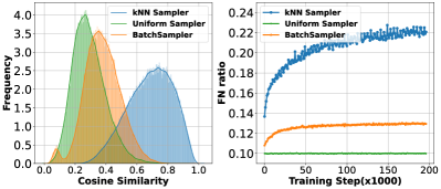
Figure 4. Cosine similarity and percentage of false negatives among various mini-batch sampling methods on CIFAR10.

5.3. Empirical Criterion for BatchSampler

BatchSampler modulates the hardness of the sampled batch by two important parameters $M$ and $\alpha$ to achieve better performance on three modalities. To analyze the impact of these, we vary the $M$ and $\alpha$ in the range of $\{500,1000,2000,4000,6000\}$ and $\{0.1,0.3,0.5,0.7\}$ respectively, and apply SimCLR, SimCSE and GraphCL as backones. We summarize the performance of BatchSampler with different $M$ and $\alpha$ in Table 4. It shows that in most cases, the performance of the model peaks when $M=1000$ but plumbs quickly with the increase of $M$. Such phenomena are consistent with the intuition that higher $M$ raises the probability of selecting similar instances as neighbors, but the sampler will be more likely to draw the mini-batch with false negatives, degrading the performance.

Besides, to better understand the effect of $\alpha$, we visualize the histograms of cosine similarity for all pairs from a sampled batch after training and plot the corresponding percentage of false negatives during training on CIFAR10 (See Figure 5). We can observe that $\alpha$ moving from 0.1 to 0.7 causes cosine similarities to gradually skew left, but introduces more false negatives in the batch, creating a trade-off. This phenomenon indicates that the sampler with a higher $\alpha$ sample more frequently within a local neighborhood, which is more likely to yield similar pairs. A similar phenomenon can also be found on CIFAR100 (See Appendix B.5). However, as training progresses, the instances of the same class tend to group together, increasing the probability of collecting false negatives. To find the best balance, we linearly decay $\alpha$ from 0.2 to 0.05 as the training epoch increases, which is presented as $0.2\sim 0.05$ in Table 4. It can be found that this dynamic strategy achieves the best performance in all cases except SimCSE which only trains for one epoch. Interestingly, SimCSE achieves the best performance by a large margin when $\alpha=0.7$ since hard negatives can alleviate the distribution issue brought by the pre-trained language model. More analysis can be found in Section 5.1 and Appendix B.6.

Criterion. From the above analysis, the suggested $M$ would be 500 for the small-scale dataset, and 1000 for the larger dataset. The suggested $\alpha$ should be relatively high, e.g., 0.7, for the pre-trained language model-based method. Besides, dynamic decay $\alpha$, e.g., 0.2 to 0.05, is the best strategy for the other methods. Such an empirical criterion provides critical suggestions for selecting the appropriate $M$ and $\alpha$ to modulate the hardness of the sampled batch.

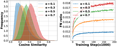
Figure 5. Cosine similarity and percentage of false negatives among various restart probabilities on CIFAR10.

5.4. Efficiency Analysis

Here, we introduce three metrics to analyze the time cost of mini-batch sampling by BatchSampler: (1) Batch Sampling Cost ($\text{Cost}_{S}$) is the average time of RWR taken to sample a mini-batch from a proximity graph; (2) Proximity Graph Construction Cost ($\text{Cost}_{G}$) refers to the time consumption of BatchSampler for constructing a proximity graph; (3) Batch Training Cost ($\text{Cost}_{T}$) is the average time taken by the encoder to forward and backward; (4) Proximity Graph Construction Amortized Cost ($\text{Cost}_{G/t}$) is the ratio of $\text{Cost}_{G}$ to the graph update interval $t$. The time cost of BatchSampler is shown in Table 5, from which we make the following observations: (1) Sampling a mini-batch $\text{Cost}_{S}$ takes an order of magnitude less time than training with a batch $\text{Cost}_{T}$ at most cases. (2) Although it takes $100s$ for BatchSampler to construct a proximity graph in ImageNet, the cost shares across $t$ training steps, which take only $\text{Cost}_{G/t}=0.2$ per batch. A similar phenomenon can be found in other datasets as well. In particular, SimCSE trains for one epoch, and proximity graph is built once.

Table 5. The time cost of mini-batch sampling by BatchSampler on an NVIDIA V100 GPU.

Metric	STL10	ImageNet-100	Wikipedia	ImageNet
$\text{Cost}_{S}$	0.013s	0.015s	0.005	0.15s
$\text{Cost}_{G}$	2s	3s	79s	100s
$\text{Cost}_{T}$	0.55s	1.1s	0.08s	1.1s
$\text{Cost}_{G/t}$	0.02($t=100$)	0.03($t=100$)	0.005($t=15625$)	0.2($t=500$)

5.5. Further Analysis

Strategies of Proximity Graph Sampling. We conduct experiments to explore different choices of graph sampling methods, including (1) Depth First Search (DFS); (2) Breadth First Search (BFS); (3) Random Walk (RW); (4) Random Walk with Restart (RWR). Table 6 presents an overall performance comparison with different graph sampling methods. As expected, RWR consistently achieves better performance since it samples hard yet true negatives within a local cluster on proximity graph. Besides, we illustrate the histograms of cosine similarity for all pairs from a sampled batch and plot the corresponding percentage of false negatives during training in Figure 6. It can be observed that although BFS brings the most similar pairs in the mini-batch, it performs worse than the original SimCLR since it introduces substantial false negatives. While having a slightly lower percentage of false negatives than RWR, DFS, and RW do not exhibit higher performance since they are unable to collect the hard negatives in the mini-batch. The restart property allows RWR to exhibit a mixture of DFS and BFS, which can flexibly modulate the hardness of the sampled batch and find the best balance between hard negatives and false negatives.

Table 6. Overall performance comparison with different graph sampling methods.

Method	Vision			Language	Graphs
	CIFAR10	CIFAR100	STL10	Wikipedia	IMDB-B	COLLAB
BFS	91.03	65.15	77.08	74.39	70.48	69.98
DFS	92.14	68.29	83.05	73.40	71.12	70.60
RW	92.28	68.33	83.54	75.56	71.26	70.72
RWR	92.54	68.68	84.38	76.69	71.90	71.48

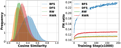
Figure 6. Histograms of cosine similarity and percentage of false negatives in a batch using different sampling methods.

Proximity Graph vs. kNN Graph. To demonstrate the effectiveness of proximity graph, we do an ablation study by replacing proximity graph with kNN graph which directly selects $k$ neighbors with the highest scores for each instance from the whole dataset. The neighbor number $k$ is 100 by default. The comparison results are shown in Table 7, from which we can observe that proximity graph outperforms the kNN graph by a margin. BatchSampler with kNN graph even performs worse than the original contrastive learning method because of the false negatives.

Table 7. Performance comparison of different graph construction methods.

Method	Vision		Language	Graphs
	CIFAR10	CIFAR100	Wikipedia	IMDB-B	COLLAB
Default	92.13	68.14	75.60	70.90	70.62
kNN graph	90.47	62.67	75.13	70.10	69.96
proximity graph	92.54	68.68	76.69	71.90	71.48

To develop an intuitive understanding of how proximity graph alleviates the false negative issue, Figure 7 plots the changing curve of false negative ratio in a batch. The results show that the proximity graph could discard the false negative significantly: by the end of the training, kNN will introduce more than 22% false negatives in a batch, while the proximity graph brings about 13% on CIFAR10. A similar phenomenon can also be found on CIFAR100.

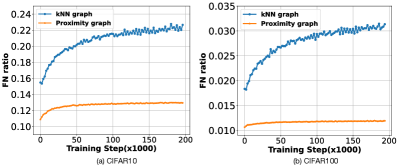
Figure 7. Percentage of false negatives using different graph building methods over the training step.

6. Conclusion

In this paper, we study the problem of mini-batch sampling for in-batch contrastive learning, which aims to globally sample mini-batches of hard-to-distinguish instances. To achieve this, we propose BatchSampler to perform mini-batch sampling as a walk on the constructed proximity graph. Specifically, we design the proximity graph to control the pairwise similarity among instances and leverage random walk with restart (RWR) on the proximity graph to form a batch. We theoretically and experimentally demonstrate that BatchSampler can balance kNN Sampler and Uniform Sampler. Besides, we conduct experiments with 5 representative contrastive learning algorithms on 3 modalities (e.g. vision, language, and graphs) to evaluate our proposed BatchSampler, demonstrating that BatchSampler can consistently achieve performance improvements.

Acknowledgements. This work was supported by Technology and Innovation Major Project of the Ministry of Science and Technology of China under Grant 2020AAA0108400 and 2020AAA0108402, NSF of China for Distinguished Young Scholars (61825602), NSF of China (62276148), and a research fund from Zhipu.AI.

Appendix A Algorithm Details

Here we present the details of Proximity Graph Construction and Random Walk with Restart, as shown in Algorithm 2 and Algorithm 3 respectively.

Input: Dataset $\mathcal{D}=\{x_{i}\}$, Candidate set size $M$, Neighbor number $K$;

Output: A proximity graph $G$;

for $v$ in $\mathcal{D}$ do

       Randomly select $M$ neighbor candidates from $\mathcal{D}$;

       Select the $K$ closest candidates $\mathcal{N}_{v}$ by Eq. 3;

       $G[v]\leftarrow\mathcal{N}_{v}$;

end for

return $G$

Algorithm 2 Proximity Graph Construction

Input: Proximity graph $G=\{\mathcal{V},\mathcal{E}\}$, seed node $u$, restart probability $\alpha$, number of sampled node $B$;

Output: A sampled node set $\mathcal{S}$;

$\mathcal{S}\leftarrow\{\},v\leftarrow u$;

while $\text{len}(\mathcal{S})<B$ do

       if $v$ not in $\mathcal{S}$ then

             $\mathcal{S}$.insert($v$)

       end if

      Sample $r$ from Uniform distribution $U(0,1)$;

       if $r<\alpha$ then

             $v\leftarrow u$;

       end if

      else

             Randomly sample $\hat{v}$ from $v$’s neighbors;

             $v\leftarrow\hat{v}$;

       end if

      

end while

return $\mathcal{S}$

Algorithm 3 Random Walk with Restart(RWR)

Appendix B Additional Experiments

B.1. Extensive studies on Vision

Here we evaluate the BatchSampler on two small-scale (CIFAR10, CIFAR100) and two medium-scale (STL10, ImageNet-100) benchmark datasets, and equip DCL (Chuang et al., 2020) and HCL (Robinson et al., 2021) with BatchSampler to investigate its generality. Experimental results in Table 8 show that BatchSampler can consistently improve SimCLR and its variants on all the datasets, with an absolute gain of 0.3%$\sim$2.5%. We also can observe that the improvement is greater on medium-scale datasets than on small-scale datasets. Specifically, the model equipped with HCL and BatchSampler achieves a significant improvement (6.23%) on STL10 over the original SimCLR.

B.2. Experiments with Roberta on Language

We also apply BatchSampler to the SimCSE with the pretrained RoBERTa (Liu et al., 2019) and present the results in Table 9. Similar to the results of BERT, BatchSampler can consistently improve the performance of the baseline model. Besides, as discussed in Section 5.1 and Section B.6, the hard negative sampled by BatchSampler explicitly can alleviate the low distribution gap between positive score and negative score distribution caused by the pretrained language model, alleviating the performance degradation of DCL and HCL.

Table 8. Overall performance comparison on image classification task in terms of Top-1 Accuracy.

Method	CIFAR10	CIFAR100	STL10	ImageNet-100
SimCLR	92.13	68.14	83.26	59.30
w/ kNN Sampler	90.16	62.30	79.25	57.70
w/ BatchSampler	92.54	68.68	84.38	60.80
DCL	92.28	68.52	84.92	59.90
w/ BatchSampler	92.74	68.91	86.39	60.14
HCL	92.39	68.92	88.20	60.60
w/ BatchSampler	92.41	69.13	89.49	61.50

Table 9. Performance comparison for sentence embedding learning based on RoBERTa.

Method	STS12	STS13	STS14	STS15	STS16	STS-B	SICK-R	Avg.
SimCSE-RoBERTabase	67.90	80.91	73.14	80.58	80.74	80.26	69.87	76.20
w/ kNN Sampler	68.78	79.49	73.34	81.05	80.15	77.09	67.18	75.30
w/ BatchSampler	68.29	81.96	73.86	82.16	80.94	80.77	69.30	76.75
DCL-RoBERTabase	66.60	79.16	71.05	80.40	77.76	77.94	67.57	74.35
w/ kNN Sampler	65.39	79.04	69.71	78.37	75.98	74.72	64.39	72.51
w/ BatchSampler	65.53	80.09	71.00	80.64	78.35	77.75	67.52	74.41
HCL-RoBETabase	67.20	80.47	72.44	80.88	80.57	78.79	67.98	75.49
w/ kNN Sampler	65.99	77.32	73.71	80.59	79.78	77.70	65.40	74.36
w/ BatchSampler	66.01	80.79	73.58	81.25	80.66	79.22	68.52	75.72

Table 10. Experiment results for graph classification task under LIBSVM (Chang and Lin, 2011) classifier.

Method	Dataset	IMDB-B	IMDB-M	COLLAB	REDDIT-B	PROTEINS	MUTAG	NCI1
Supervised	GIN	75.1$\pm$5.1	52.3$\pm$2.8	80.2$\pm$1.9	92.4$\pm$2.5	76.2$\pm$2.8	89.4$\pm$5.6	82.7$\pm$1.7
	DiffPool	72.6$\pm$3.9	-	78.9$\pm$2.3	92.1$\pm$2.6	75.1$\pm$3.5	85.0$\pm$10.3	-
Graph Kernels	WL	72.30$\pm$3.44	46.95$\pm$0.46	-	68.82$\pm$0.41	72.92$\pm$0.56	80.72$\pm$3.00	80.31$\pm$0.46
	DGK	66.96$\pm$0.56	44.55$\pm$0.52	-	78.04$\pm$0.39	73.30$\pm$0.82	87.44$\pm$2.72	80.31$\pm$0.46
Self-supervised	graph2vec	71.10$\pm$0.54	50.44$\pm$0.87	-	75.78$\pm$1.03	73.30$\pm$2.05	83.15$\pm$9.25	73.22$\pm$1.81
	infograph	73.03$\pm$0.87	49.69$\pm$0.53	70.65$\pm$1.13	82.50$\pm$1.42	74.44$\pm$0.31	89.01$\pm$1.13	76.20$\pm$1.06
	JOAO	70.21$\pm$3.08	49.20$\pm$0.77	69.50$\pm$0.36	85.29$\pm$1.35	74.55$\pm$0.41	87.35$\pm$1.02	78.07$\pm$0.47
	GCC	72.0	49.4	78.9	89.9	-	-	-
	InfoGCL	75.10$\pm$0.90	51.40$\pm$0.80	-	-	-	91.20$\pm$1.30	-
	GraphCL	70.90$\pm$0.53	48.48$\pm$0.38	70.62$\pm$0.23	90.54$\pm$0.25	74.39$\pm$0.45	86.80$\pm$1.34	77.87$\pm$0.41
	GraphCL + BatchSampler	71.90$\pm$0.46	48.93$\pm$0.28	71.48$\pm$0.28	90.88$\pm$0.16	75.04$\pm$0.67	87.78$\pm$0.93	78.93$\pm$0.38
	MVGRL	74.20$\pm$0.70	51.20$\pm$0.50	-	84.50$\pm$0.60	-	89.70$\pm$1.10	-
	MVGRL + BatchSampler	76.70$\pm$0.35	52.40$\pm$0.39	-	87.47$\pm$0.79	-	91.13$\pm$0.81	-

B.3. Comparison with baselines on Graphs

In Table 10, we comprehensively compare different kinds of baselines on graph classification tasks, including the unsupervised graph learning methods (Xu et al., 2018; Ying et al., 2018), graph kernel methods (Shervashidze et al., 2011; Yanardag and Vishwanathan, 2015), and self-supervised graph learning methods (Qiu et al., 2020; You et al., 2020; Hassani and Khasahmadi, 2020; Narayanan et al., 2017; Sun et al., 2019; You et al., 2021; Xu et al., 2021). It can be found that InfoGCL achieves state-the-of-art performance among the self-supervised methods, and even outperforms the supervised methods on some datasets. BatchSampler can consistently improve the performance of both GraphCL and MVGRL on all the datasets, demonstrating the effectiveness of global hard negatives. Benefiting from the performance gain brought by BatchSampler, MVGRL achieves the best performance on 4 datasets, outperforming InfoGCL and supervised methods.

B.4. Performance Analysis on CIFAR100

Here we compare the Uniform Sampler, kNN Sampler, and BatchSampler regarding cosine similarity, false negatives, and performance comparison on CIFAR100. Specifically, we show the histogram of cosine similarity for all pairs in a sampled batch, the false negative ratio of the mini-batch, and performance comparison between BatchSampler and other two sampling strategies (e.g. Uniform Sampler and kNN Sampler) in Figure 8. It can be found that BatchSampler exhibits a balance of Uniform Sampler and kNN Sampler, which can sample the hard negative pair but only brings a slightly greater number of false negatives than Uniform Sampler. More analysis can be found in Section 5.2.

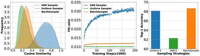
Figure 8. Cosine similarity, false negative ratio, and performance comparison on CIFAR100.

B.5. Restart Probability Analysis on CIFAR100

Figure 9 shows cosine similarities and percentage of false negatives in the sampled batch among various restart probabilities $\alpha$ on CIFAR100. It can be observed that cosine similarities gradually skew left with the increase of $\alpha$ from $0.1$ to $0.7$, indicating the higher $\alpha$ brings about more hard negative instances similar to positive anchor. However, higher $\alpha$ suffers from more serious FN issues, which significantly increases the percentage of false negatives in the sampled batch. Thus, we linearly decay $\alpha$ from $0.2$ to $0.05$, achieving a trade-off between hard negatives and false negatives. More analyses are discussed in Section 5.3.

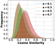
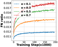
Figure 9. Cosine similarities and percentage of false negatives among various restart probabilities.

B.6. Similarity Comparison Between Positive and Negative Pairs

To explain the performance degradation of DCL and HCL objectives, we select 12 representative mini-batches and plot the cosine similarity histogram of positive and negative pairs on BERT (top) and RoBERTa (bottom) in Figure 10. We observe the following: (1) At the start of and throughout the training, the positive pairs are assigned a high cosine similarity (around 0.9) by the pretrained language model; (2) The negative similarities begin with a relatively high score and gradually skew left because of the self-supervised learning. Such phenomenon is consistent to Zhou et al. (2022). DCL and HCL which leverage the difference between positive and negative similarity to reweight the negative scores are inapplicable since the low distribution gap between positive and negative similarities will lead to homogeneous weighting in the objective.

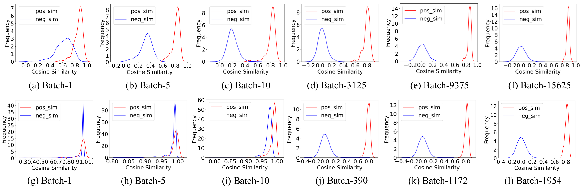
Figure 10. Histograms of cosine similarity on BERT (top) and RoBERTa (bottom).

B.7. Impact of Sampling Method on CIFAR100

We conduct different strategies of proximity graph sampling on CIFAR100 to investigate the impact of sampling methods. As shown in Figure 11, BFS achieves more similar pairs in the sampled batch compared with other proximity graph sampling methods but it introduces a higher percentage of false negatives, which obviously degrades the downstream performance. Conversely, DFS explores paths far away from the selected central node, which can not guarantee that the sampled path (i.e. batch) is within a local cluster. Thus, we theoretically leverage RWR to flexibly modulate the hardness of the sampled batch and achieve a balance between hard negatives and false negatives.

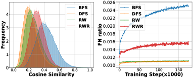
Figure 11. Histograms of cosine similarity and Percentage of false negative of all pairs in a batch for embeddings trained using different sampling methods.

B.8. Parameter Analysis

B.8.1. Batchsize $B$

To analyze the impact of the batchsize $B$, we vary $B$ in the range of {16, 32, 64, 128, 256} and summarize the results in Table 11. In vision modality, it can be found that a larger batchsize leads to better results, which is consistent with the previous studies (Chen et al., 2020; He et al., 2020; Kalantidis et al., 2020). In language domain, BatchSampler reaches its optimum at $B=64$, which aligns with the results in SimCSE (Gao et al., 2021). For graphs, we can observe that the performance improves slightly with increasing batch size.

Table 11. Performance comparison of different batchsize $B$.

$B$	Vision			Language	Graphs
	CIFAR10	CIFAR100	STL10	Wikipedia	IMDB-B	COLLAB
16	79.93	46.69	56.31	76.26	71.50	71.32
32	84.64	56.24	68.61	74.16	71.60	71.40
64	89.09	61.30	74.24	76.69	71.65	71.42
128	91.03	65.96	82.56	76.64	71.83	71.48
256	92.54	68.68	84.38	76.11	71.90	71.35

B.8.2. Impact of Neighbor Number $K$

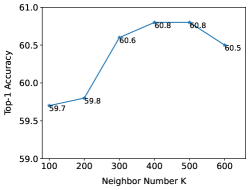
Figure 12. Impact of neighbor number $K$.

In Figure 12, we investigate the impact of the neighbor number $K$ on ImageNet-100 dataset with the default BatchSampler setting. We observe an absolute improvement of 1.1% with the increasing size of neighbors. Specifically, model achieves an absolute performance gain of 0.9% from $K=100$ to $K=300$, while only obtaining 0.2% from $K=300$ to $K=500$. Such experimental results are consistent with our prior philosophy, in which sampling more neighbors always increases the scale of proximity graph and urges BatchSampler to explore smaller-scope local clusters (i.e. sample harder negatives within a batch), leading to a significant improvement in performance at first. However, performance degrades after reaching the optimum, because larger $K$ introduces more easy negatives.

B.8.3. Proximity Graph Update Interval $t$

Proximity graph will be updated per $t$ training iterations, and to analyze the impact of $t$, we vary $t$ in the range of {50,100,200,400} for vision and {10,25,50,100} for graphs respectively. Table 12 summarizes the experimental results on different update interval $t$. It can be observed that update intervals that are too short or too long will degrade the performance. The possible reason is that sampling on a proximity graph that is frequently updated results in unstable learning of the model. Besides, the distribution of instances in the embedding space will change during the training process, resulting in a shift in hard negatives. As a result, after a few iterations, the lazy-updated graph cannot adequately capture the similarity relationship.

Table 12. Performance comparison with different update interval $t$ on vision and graph modality.

	Update Interval $t$	50	100	200	400
Vision	CIFAR10	92.29	92.54	92.34	92.26
	CIFAR100	68.37	68.68	67.83	68.59
	Update Interval $t$	10	25	50	100
Graphs	IMDB-B	71.30	71.90	71.40	71.10
	COLLAB	71.06	70.36	71.48	70.62

B.9. Training Curve

We plot the training curves on STL10 and ImageNet-100 respectively. As shown in Figure 13, on STL10 dataset, BatchSampler takes only about 600 epochs to achieve a similar performance as the original SimCLR, which takes 1000 epochs. A similar phenomenon can be seen on ImageNet-100. All these results manifest that BatchSampler can bring model better and faster learning.

(a) STL10

(b) ImageNet-100

Figure 13. Training curves for image classification task on STL10 and ImageNet-100.

Appendix C InfoNCE Objective and its Variants

Here we describe in detail the objective functions of three in-batch contrastive learning methods, including SimCLR (Chen et al., 2020), GraphCL (You et al., 2020) and SimCSE (Gao et al., 2021). Besides, we cover two variants, i.e., DCL (Chuang et al., 2020) and HCL (Robinson et al., 2021), which are also applied in the experiments.

C.1. SimCLR

SimCLR (Chen et al., 2020) first uniformly draws a batch of instances $\{x_{1}...\ x_{B}\}\subset\mathcal{D}$, then augments the instances by two randomly sampled augmentation strategies $f_{aug}(\cdot),f^{\prime}_{aug}(\cdot)\sim\mathcal{T}$, resulting in $2B$ data points. Two augmented views $(x_{i},x_{i+B})$ of the same image are treated as a positive pair, while the other $2(B-1)$ examples are negatives. The objective function applied in SimCLR for a positive pair $(x_{i},x_{i+B})$ is formulated as:

(16) $$\ell_{i,i+B}=-\log\frac{e^{f(x_{i})^{T}f(x_{i+B})/\tau}}{\sum_{j\neq i}^{2B}e^{f(x_{i})^{T}f(x_{j})/\tau}},$$

where $\tau$ is the temperature and $f(\cdot)$ is the encoder. The loss is calculated for all positive pairs in a mini-batch, including $(x_{i},x_{i+B})$ and $(x_{i+B},x_{i})$. It can be found that SimCLR takes all $2(B-1)$ augmented instances within a mini-batch as negatives.

C.2. GraphCL and SimCSE

Similar to SimCLR, the objective function of GraphCL (You et al., 2020) and SimCSE (Gao et al., 2021) is defined on the augmented instance pairs within a mini-batch. Given a sampled mini-batch $\{x_{1}...\ x_{B}\}\subset\mathcal{D}$, both GraphCL and SimCSE apply data augmentation to obtain positive pairs, and the loss function for a positive pair $(x_{i},x_{i}^{+})$ can be formulated as:

(17) $$\ell_{i}=-\log\frac{e^{f(x_{i})^{T}f(x_{i}^{+})/\tau}}{\sum_{j=1}^{B}e^{f(x_{i})^{T}f(x_{j}^{+})/\tau}}.$$

Compared with the SimCLR, GraphCL and SimCSE only take the other $B-1$ augmented instances as negatives.

C.3. DCL and HCL

DCL (Chuang et al., 2020) and HCL (Robinson et al., 2021) are two variants of InfoNCE objective function, which aim to alleviate the false negative issue or mine the hard negatives by reweighting the negatives in the objective. The main idea behind them is using the positive distribution to correct for the negative distribution.

For simplicity, we annotate the positive score $e^{f(x_{i})^{T}f(x_{i}^{+})/\tau}$ as $pos$, and negative score $e^{f(x_{i})^{T}f(x_{j}^{+})/\tau}$ as $neg_{ij}$. Given a mini-batch and a positive pair $(x_{i},x_{i}^{+})$, the reweighting negative distribution proposed in DCL and HCL are:

(18) $$\max{\left(\sum_{j=1}^{B}\frac{-N_{neg}\times\tau^{+}\times pos+\lambda_{ij}\times neg_{ij}}{1-\tau^{+}},e^{-1/\tau}\right)},$$

where $N_{neg}$ is the number of the negatives in mini-batch, $\tau^{+}$ is the class probability, $\tau$ is the temperature, and $\lambda_{ij}$ is concentration parameter which is simply set as 1 in DCL or calculated as $\lambda_{ij}=\frac{\beta\times neg_{ij}}{\sum neg_{ij}/N_{neg}}$ in HCL. All of $\tau^{+},\tau,\beta$ are tunable hyperparameters. The insight of Eq.18 is that the negative pair with a score closer to a positive score will be assigned a lower weight in the loss function. In other words, the similarity difference between positive and negative pairs dominates the weighting function.

Appendix D Dataset Details

For image representation learning, we adopt five benchmark datasets, comprising CIFAR10, CIFAR100, STL10, ImageNet-100 and ImageNet ILSVRC-2012 (Russakovsky et al., 2015). Information on the statistics of these datasets is summarized in Table 13. For graph-level representation learning, we conduct experiments on IMDB-B, IMDB-M, COLLAB, REDDIT-B, PROTEINS, MUTAG, and NCI1 (Yanardag and Vishwanathan, 2015), the details of which are presented in Table 14. For text representation learning, we evaluate the method on a one-million English Wikipedia dataset which is used in the SimCSE and can be downloaded from HuggingFace repository.

Table 13. Statistics of datasets for image classification task.

Datasets	CIFAR10	CIFAR100	STL10	ImageNet-100	ImageNet
#Train	50,000	50,000	105,000	130,000	1,281,167
#Test	10,000	10,000	8,000	50,00	50,000
#Classes	10	100	10	100	1,000

Table 14. Statistics of datasets for graph-level classification task.

Datasets	IMDB-B	IMDB-M	COLLAB	REDDIT-B	PROTEINS	MUTAG	NCI1
#Graphs	1,000	1,500	5,000	2,000	1,113	188	4,110
#Classes	2	3	3	2	2	2	2
Avg. #nodes	19.8	13.0	74.5	429.7	39.1	17.9	29.8

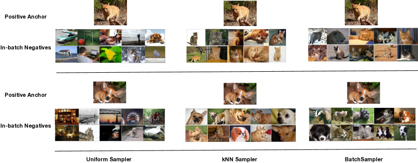
Figure 14. Case study of the negatives sampled by Uniform Sampler, kNN Sampler, and BatchSampler based on the encoder trained for 100 epochs on ImageNet. Given an anchor image (Cat or Dog), (Left) in-batch negatives sampled by Uniform Sampler, (Middle) in-batch negatives sampled by kNN Sampler, and (Right) in-batch negatives sampled by BatchSampler based on proximity graph.

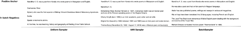
Figure 15. Case study of the negatives sampled by Uniform Sampler, kNN Sampler, and BatchSampler on language domain.

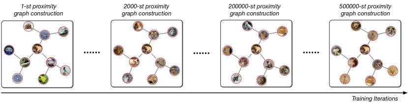
Figure 16. A visualization of the process of updating the proximity graph.

Appendix E Experimental Details

E.1. Image Representations

In image domain, we apply SimCLR (Chen et al., 2020) and MoCo v3 (Chen et al., 2021) as the baseline method, with ResNet-50 (He et al., 2016) as an encoder to learn image representations. The feature map generated by ResNet-50 block is projected to a 128-D image embedding via a two-layer MLP (2048-D hidden layer with ReLU activation function). Besides, the output vector is normalized by $l_{2}$ normalization (Wu et al., 2018). We employ two sampled data augmentation strategies to generate positive pairs and implicitly use other examples in the same mini-batch as negative samples.

For CIFAR10, CIFAR100 and STL10, all models are trained for 1000 epochs with the default batch size $B$ of 256. We use the Adam optimizer (Kingma and Ba, 2015) with a learning rate of 0.001 for optimization. The temperature parameter is set as 0.5 and the dimension of image embedding is set as 128. For ImageNet-100 and ImageNet, we train the models with 100 and 400 epochs respectively, and use LARS optimizer (You et al., 2019) with a learning rate of $0.3\times B/256$ and weight decay of $10^{-6}$. Here, the batch size is set as 2048 for ImageNet and 512 for ImageNet-100, respectively. We fix the temperature parameter as 0.1 and the image embedding dimension as 128. After the unsupervised learning, we train a supervised linear classifier for 100 epochs on top of the frozen learned representations.

As for BatchSampler, we update the proximity graph per 100 training iterations. We fix the number of neighbors $K$ as 100 for CIFAR10, CIFAR100 and STL10. The size of the neighbor candidate set $M$ is set as 1000 for CIFAR100 and STL10, and 500 for CIFAR10. Besides, the initial restart probability $\alpha$ of RWR (Random Walk with Restart) is set to 0.2 and decays linearly to 0.05 with the training process. For ImageNet-100 and ImageNet, we keep $M$ as 1000 and $K$ as 500. The restart probability $\alpha$ is fixed as 0.1.

E.2. Graph Representations

In graph domain, we use the GraphCL (You et al., 2020) framework as the baseline and GIN (Xu et al., 2018) as the backbone. We run BatchSampler 5 times with different random seeds and report the mean 10-fold cross-validation accuracy with variance. We apply Adam optimizer (Kingma and Ba, 2015) with a learning rate of 0.01 and 3-layer GIN with a fixed hidden size of 32. We set the temperature as 0.2 and gradually decay the restart probability of RWR ($0.2\sim 0.05$). Proximity graph will be updated after $t$ iterations. The overall hyperparameter settings on different datasets are summarized in Table 15.

Table 15. Hyperparameter settings for graph-level representation learning.

Datasets	IMDB-B	IMDB-M	COLLAB	REDDIT-B	PROTEINS	MUTAG	NCI1
$B$	256	128	128	128	128	128	128
Epoch	100	50	20	50	20	20	20
$t$	25	25	50	50	50	50	50
$M$	500	500	1,000	500	500	100	1000
$K$	100	100	100	100	100	50	100

E.3. Text Representations

In text domain, we use SimCSE (Gao et al., 2021) as the baseline method and adopt the pretrained BERT and RoBERTa provided by HuggingFace for sentence embedding learning. Following the training setting of SimCSE, we train the model for one epoch in an unsupervised manner and evaluate it on 7 STS tasks. Proximity graph will be only built once based on the pretrained language models before training. For BERT, we set the batch size to 64 and the learning rate to $3\times 10^{-5}$. For RoBERTa, the batch size is set as 512 and the learning rate is fixed as $10^{-5}$. We keep the temperature as 0.05, the number of neighbor candidates $M$ as 1000, the number of neighbors $K$ as 500, and the restart probability $\alpha$ as 0.7 for both BERT and RoBERTa.

E.4. Case Study

To give an intuitive impression of the mini-batch sampled by BatchSampler, we show some real cases of the negatives sampled by Uniform Sampler, kNN Sampler, and BatchSampler in Figure 14. For a given anchor (a cat or a dog), we apply Uniform Sampler, kNN Sampler, and BatchSampler to draw a mini-batch of images, and randomly pick 10 images from the sampled batch to show in-batch negatives for the positive anchor. Obviously, compared with Uniform Sampler, the images sampled by BatchSampler are more semantically relevant to the anchor in terms of texture, background, or appearance. Furthermore, kNN Sampler introduces so many false negatives that belong to the same class with positive anchor, degrading downstream performance. Thus, the proposed BatchSampler can effectively balance the exploitation of hard negatives and the FN issue.

Furthermore, we provide a visualization of language to demonstrate the effectiveness and generalizability of BatchSampler in Figure 15. Here, we also take a vision as an example and visualize the process of updating the proximity graph in Figure 16. We maintain the default starting image and randomly sample a predetermined number of neighboring images at a specific iteration in each proximity graph.

References

- (1)
- Agirre et al. (2015) Eneko Agirre, Carmen Banea, Claire Cardie, Daniel Cer, Mona Diab, Aitor Gonzalez-Agirre, Weiwei Guo, Inigo Lopez-Gazpio, Montse Maritxalar, Rada Mihalcea, et al. 2015. Semeval-2015 task 2: Semantic textual similarity, english, spanish and pilot on interpretability. In SemEval’15. 252–263.
- Agirre et al. (2014) Eneko Agirre, Carmen Banea, Claire Cardie, Daniel M Cer, Mona T Diab, Aitor Gonzalez-Agirre, Weiwei Guo, Rada Mihalcea, German Rigau, and Janyce Wiebe. 2014. SemEval-2014 Task 10: Multilingual Semantic Textual Similarity. In SemEval’14. 81–91.
- Agirre et al. (2016) Eneko Agirre, Carmen Banea, Daniel Cer, Mona Diab, Aitor Gonzalez Agirre, Rada Mihalcea, German Rigau Claramunt, and Janyce Wiebe. 2016. Semeval-2016 task 1: Semantic textual similarity, monolingual and cross-lingual evaluation. In SemEval’16.
- Agirre et al. (2012) Eneko Agirre, Daniel Cer, Mona Diab, and Aitor Gonzalez-Agirre. 2012. Semeval-2012 task 6: A pilot on semantic textual similarity. In SemEval’12. 385–393.
- Agirre et al. (2013) Eneko Agirre, Daniel Cer, Mona Diab, Aitor Gonzalez-Agirre, and Weiwei Guo. 2013. * SEM 2013 shared task: Semantic textual similarity. In SemEval’13. 32–43.
- Andersen et al. (2006) Reid Andersen, Fan Chung, and Kevin Lang. 2006. Local graph partitioning using pagerank vectors. FOCS’06.
- Avrachenkov et al. (2014) Konstantin Avrachenkov, Remco van der Hofstad, and Marina Sokol. 2014. Personalized pagerank with node-dependent restart. In WAW’14. 23–33.
- Caron et al. (2020) Mathilde Caron, Ishan Misra, Julien Mairal, Priya Goyal, Piotr Bojanowski, and Armand Joulin. 2020. Unsupervised learning of visual features by contrasting cluster assignments. In NIPS’20. 9912–9924.
- Chang and Lin (2011) Chih-Chung Chang and Chih-Jen Lin. 2011. LIBSVM: a library for support vector. TIST’11 (2011), 1–27.
- Chen et al. (2020) Ting Chen, Simon Kornblith, Mohammad Norouzi, and Geoffrey Hinton. 2020. A simple framework for contrastive learning of visual representations. In ICML’20. PMLR, 1597–1607.
- Chen et al. (2021) Xinlei Chen, Saining Xie, and Kaiming He. 2021. An empirical study of training self-supervised vision transformers. In ICCV’21. 9640–9649.
- Chuang et al. (2020) Ching-Yao Chuang, Joshua Robinson, Lin Yen-Chen Antonio Torralba, and Stefanie Jegelka. 2020. Debiased Contrastive Learning. In NIPS’20.
- Chung and Tsiatas (2010) Fan Chung and Alexander Tsiatas. 2010. Finding and visualizing graph clusters using pagerank optimization. In WAW’10. 86–97.
- Chung and Zhao (2010) Fan Chung and Wenbo Zhao. 2010. PageRank and random walks on graphs. In Fete of combinatorics and computer science. 43–62.
- Devlin et al. (2019) Jacob Devlin, Ming-Wei Chang, Kenton Lee, and Kristina Toutanova. 2019. BERT: Pre-training of Deep Bidirectional Transformers for Language Understanding. In NAACL’19. 4171–4186.
- Gao et al. (2021) Tianyu Gao, Xingcheng Yao, and Danqi Chen. 2021. Simcse: Simple contrastive learning of sentence embeddings. EMNLP’21 (2021).
- Grover and Leskovec (2016) Aditya Grover and Jure Leskovec. 2016. node2vec: Scalable feature learning for networks. In KDD’16. 855–864.
- Gutmann and Hyvärinen (2010) Michael Gutmann and Aapo Hyvärinen. 2010. Noise-Contrastive Estimation: A new estimation principle for unnormalized statistical models. In AISTATS’10. 297–304.
- Hassani and Khasahmadi (2020) Kaveh Hassani and Amir Hosein Khasahmadi. 2020. Contrastive multi-view representation learning on graphs. In International conference on machine learning. PMLR, 4116–4126.
- He et al. (2020) Kaiming He, Haoqi Fan, Yuxin Wu, Saining Xie, and Ross Girshick. 2020. Momentum contrast for unsupervised visual representation learning. In CVPR’20.
- He et al. (2016) Kaiming He, Xiangyu Zhang, Shaoqing Ren, and Jian Sun. 2016. Deep residual learning for image recognition. In CVPR’16. 770–778.
- Huang et al. (2020) Jui-Ting Huang, Ashish Sharma, Shuying Sun, Li Xia, David Zhang, Philip Pronin, Janani Padmanabhan, Giuseppe Ottaviano, and Linjun Yang. 2020. Embedding-based retrieval in facebook search. In KDD’20. 2553–2561.
- Huang et al. (2021) Tinglin Huang, Yuxiao Dong, Ming Ding, Zhen Yang, Wenzheng Feng, Xinyu Wang, and Jie Tang. 2021. MixGCF: An Improved Training Method for Graph Neural Network-based Recommender Systems. In KDD’21. 665–674.
- Huynh et al. (2022) Tri Huynh, Simon Kornblith, Matthew R Walter, Michael Maire, and Maryam Khademi. 2022. Boosting contrastive self-supervised learning with false negative cancellation. In WACV’22. 2785–2795.
- Jaiswal et al. (2020) Ashish Jaiswal, Ashwin Ramesh Babu, Mohammad Zaki Zadeh, Debapriya Banerjee, and Fillia Makedon. 2020. A survey on contrastive self-supervised learning. Technologies 9, 1 (2020), 2.
- Johnson et al. (2019) Jeff Johnson, Matthijs Douze, and Hervé Jégou. 2019. Billion-scale similarity search with GPUs. IEEE Transactions on Big Data 7, 3 (2019), 535–547.
- Kalantidis et al. (2020) Yannis Kalantidis, Mert Bulent Sariyildiz, Noe Pion, Philippe Weinzaepfel, and Diane Larlus. 2020. Hard Negative Mixing for Contrastive Learning. In NIPS’20.
- Karpukhin et al. (2020) Vladimir Karpukhin, Barlas Oğuz, Sewon Min, Patrick Lewis, Ledell Wu, Sergey Edunov, Danqi Chen, and Wen-tau Yih. 2020. Dense passage retrieval for open-domain question answering. In EMNLP’20.
- Kingma and Ba (2015) Diederik P Kingma and Jimmy Ba. 2015. Adam: A method for stochastic optimization. In ICLR’15.
- Knuth (1997) Donald Ervin Knuth. 1997. The art of computer programming: Fundamental Algorithms. Vol. 1. Pearson Education.
- Liu et al. (2019) Yinhan Liu, Myle Ott, Naman Goyal, Jingfei Du, Mandar Joshi, Danqi Chen, Omer Levy, Mike Lewis, Luke Zettlemoyer, and Veselin Stoyanov. 2019. Roberta: A robustly optimized bert pretraining approach. arXiv preprint arXiv:1907.11692 (2019).
- Marelli et al. (2014) Marco Marelli, Stefano Menini, Marco Baroni, Luisa Bentivogli, Raffaella Bernardi, and Roberto Zamparelli. 2014. A SICK cure for the evaluation of compositional distributional semantic models. In LREC’14. 216–223.
- Meng et al. (2021) Yu Meng, Chenyan Xiong, Payal Bajaj, Paul Bennett, Jiawei Han, and Xia Song. 2021. Coco-lm: Correcting and contrasting text sequences for language model pretraining. In NIPS’21.
- Narayanan et al. (2017) Annamalai Narayanan, Mahinthan Chandramohan, Rajasekar Venkatesan, Lihui Chen, Yang Liu, and Shantanu Jaiswal. 2017. graph2vec: Learning distributed representations of graphs. In MLG’17.
- Oord et al. (2018) Aaron van den Oord, Yazhe Li, and Oriol Vinyals. 2018. Representation learning with contrastive predictive coding. arXiv preprint arXiv:1807.03748 (2018).
- Page et al. (1999) Lawrence Page, Sergey Brin, Rajeev Motwani, and Terry Winograd. 1999. The PageRank citation ranking: Bringing order to the web. Stanford University Technical Report, (1999).
- Petar et al. (2018) Veličković Petar, William Fedus, William L. Hamilton, Pietro Liò, Yoshua Bengio, and R. Devon Hjelm. 2018. Deep graph infomax. In ICLR’19.
- Qiu et al. (2020) Jiezhong Qiu, Qibin Chen, Yuxiao Dong, Jing Zhang, Hongxia Yang, Ming Ding, Kuansan Wang, and Jie Tang. 2020. Gcc: Graph contrastive coding for graph neural network pre-training. In KDD’20. 1150–1160.
- Robinson et al. (2021) Joshua Robinson, Ching-Yao Chuang, Suvrit Sra, and Stefanie Jegelka. 2021. Contrastive Learning with Hard Negative Samples. In ICLR’21.
- Russakovsky et al. (2015) Olga Russakovsky, Jia Deng, Hao Su, Jonathan Krause, Sanjeev Satheesh, Sean Ma, Zhiheng Huang, Andrej Karpathy, Aditya Khosla, Michael Bernstein, et al. 2015. Imagenet large scale visual recognition challenge. International journal of computer vision 115, 3 (2015), 211–252.
- Shervashidze et al. (2011) Nino Shervashidze, Pascal Schweitzer, Erik Jan Van Leeuwen, Kurt Mehlhorn, and Karsten M Borgwardt. 2011. Weisfeiler-lehman graph kernels. Journal of Machine Learning Research 12, 9 (2011).
- Spielman and Teng (2013) Daniel A Spielman and Shang-Hua Teng. 2013. A local clustering algorithm for massive graphs and its application to nearly linear time graph partitioning. SIAM Journal on computing (2013).
- Sun et al. (2019) Fan-Yun Sun, Jordan Hoffmann, Vikas Verma, and Jian Tang. 2019. Infograph: Unsupervised and semi-supervised graph-level representation learning via mutual information maximization. In ICLR’20.
- Tabassum et al. (2022) Afrina Tabassum, Muntasir Wahed, Hoda Eldardiry, and Ismini Lourentzou. 2022. Hard negative sampling strategies for contrastive representation learning. arXiv preprint arXiv:2206.01197 (2022).
- Tian et al. (2017) Junfeng Tian, Zhiheng Zhou, Man Lan, and Yuanbin Wu. 2017. Ecnu at semeval-2017 task 1: Leverage kernel-based traditional nlp features and neural networks to build a universal model for multilingual and cross-lingual semantic textual similarity. In SemEval’17. 191–197.
- Tong et al. (2006) Hanghang Tong, Christos Faloutsos, and Jia-Yu Pan. 2006. Fast random walk with restart and its applications. In ICDM’06.
- Wang et al. (2021) Guangrun Wang, Keze Wang, Guangcong Wang, Philip HS Torr, and Liang Lin. 2021. Solving inefficiency of self-supervised representation learning. In ICCV’21. 9505–9515.
- Wu et al. (2020a) Mike Wu, Milan Mosse, Chengxu Zhuang, Daniel Yamins, and Noah Goodman. 2020a. Conditional negative sampling for contrastive learning of visual representations. In ICLR’21.
- Wu et al. (2021) Yawen Wu, Zhepeng Wang, Dewen Zeng, Yiyu Shi, and Jingtong Hu. 2021. Enabling on-device self-supervised contrastive learning with selective data contrast. In 2021 58th ACM/IEEE Design Automation Conference (DAC). IEEE, 655–660.
- Wu et al. (2020b) Zhuofeng Wu, Sinong Wang, Jiatao Gu, Madian Khabsa, Fei Sun, and Hao Ma. 2020b. Clear: Contrastive learning for sentence representation. arXiv preprint arXiv:2012.15466 (2020).
- Wu et al. (2018) Zhirong Wu, Yuanjun Xiong, Stella X. Yu, and Dahua Lin. 2018. Unsupervised feature learning via non-parametric instance discrimination. In CVPR’18. 3733–3742.
- Xiong et al. (2020) Lee Xiong, Chenyan Xiong, Ye Li, Kwok-Fung Tang, Jialin Liu, Paul Bennett, Junaid Ahmed, and Arnold Overwijk. 2020. Approximate nearest neighbor negative contrastive learning for dense text retrieval. In ICLR’21.
- Xu et al. (2021) Dongkuan Xu, Wei Cheng, Dongsheng Luo, Haifeng Chen, and Xiang Zhang. 2021. Infogcl: Information-aware graph contrastive learning. In NIPS’21, Vol. 34. 30414–30425.
- Xu et al. (2018) Keyulu Xu, Weihua Hu, Jure Leskovec, and Stefanie Jegelka. 2018. How powerful are graph neural networks?. In ICLR’19.
- Yanardag and Vishwanathan (2015) Pinar Yanardag and SVN Vishwanathan. 2015. Deep graph kernels. In KDD’15. 1365–1374.
- Yang et al. (2020) Zhen Yang, Ming Ding, Chang Zhou, Hongxia Yang, Jingren Zhou, and Jie Tang. 2020. Understanding negative sampling in graph representation learning. In KDD’20. 1666–1676.
- Ying et al. (2018) Zhitao Ying, Jiaxuan You, Christopher Morris, Xiang Ren, Will Hamilton, and Jure Leskovec. 2018. Hierarchical graph representation learning with differentiable pooling. In NIPS’18, Vol. 31.
- You et al. (2021) Yuning You, Tianlong Chen, Yang Shen, and Zhangyang Wang. 2021. Graph contrastive learning automated. In International Conference on Machine Learning. PMLR, 12121–12132.
- You et al. (2020) Yuning You, Tianlong Chen, Yongduo Sui, Ting Chen, Zhangyang Wang, and Yang Shen. 2020. Graph Contrastive Learning with Augmentations. In NIPS’20. 5812–5823.
- You et al. (2019) Yang You, Jing Li, Sashank Reddi, Jonathan Hseu, Sanjiv Kumar, Srinadh Bhojanapalli, Xiaodan Song, James Demmel, Kurt Keutzer, and Cho-Jui Hsieh. 2019. Large batch optimization for deep learning: Training bert in 76 minutes. arXiv preprint arXiv:1904.00962 (2019).
- Yu et al. (2020) Junchi Yu, Tingyang Xu, Yu Rong, Yatao Bian, Junzhou Huang, and Ran He. 2020. Graph information bottleneck for subgraph recognition. In ICLR’21.
- Yu et al. (2021) Junchi Yu, Tingyang Xu, Yu Rong, Yatao Bian, Junzhou Huang, and Ran He. 2021. Recognizing predictive substructures with subgraph information bottleneck. IEEE Transactions on Pattern Analysis and Machine Intelligence (2021).
- Zhang et al. (2022) Shaofeng Zhang, Meng Liu, Junchi Yan, Hengrui Zhang, Lingxiao Huang, Xiaokang Yang, and Pinyan Lu. 2022. M-Mix: Generating Hard Negatives via Multi-sample Mixing for Contrastive Learning. In Proceedings of the 28th ACM SIGKDD Conference on Knowledge Discovery and Data Mining. 2461–2470.
- Zhang et al. (2013) Weinan Zhang, Tianqi Chen, Jun Wang, and Yong Yu. 2013. Optimizing top-n collaborative filtering via dynamic negative item sampling. In SIGIR’13. 785–788.
- Zheng et al. (2021) Mingkai Zheng, Fei Wang, Shan You, Chen Qian, Changshui Zhang, Xiaogang Wang, and Chang Xu. 2021. Weakly supervised contrastive learning. In ICCV’21. 10042–10051.
- Zhou et al. (2022) Kun Zhou, Beichen Zhang, Wayne Xin Zhao, and Ji-Rong Wen. 2022. Debiased Contrastive Learning of Unsupervised Sentence Representations. In ACL’22.
- Zhu et al. (2021a) Yanqiao Zhu, Yichen Xu, Qiang Liu, and Shu Wu. 2021a. An empirical study of graph contrastive learning. arXiv preprint arXiv:2109.01116 (2021).
- Zhu et al. (2021b) Yanqiao Zhu, Yichen Xu, Feng Yu, Qiang Liu, Shu Wu, and Liang Wang. 2021b. Graph contrastive learning with adaptive augmentation. In Proceedings of the Web Conference 2021. 2069–2080.
- Šíma and Schaeffer. (2006) Jiří Šíma and Satu Elisa Schaeffer. 2006. On the np-completeness of some graph cluster measures. In International Conference on Current Trends in Theory and Practice of Computer Science.