A sketch-and-project method for solving the matrix equation $AXB=C$

Abstract

In this paper, based on an optimization problem, a sketch-and-project method for solving the linear matrix equation $AXB=C$ is proposed. We provide a thorough convergence analysis for the new method and derive a lower bound on the convergence rate and some convergence conditions including the case that the coefficient matrix is rank deficient. By varying three parameters in the new method and convergence theorems, the new method recovers an array of well-known algorithms and their convergence results. Meanwhile, with the use of Gaussian sampling, we can obtain the Gaussian global randomized Kaczmarz (GaussGRK) method which shows some advantages in solving the matrix equation $AXB=C$. Finally, numerical experiments are given to illustrate the effectiveness of recovered methods.

1 Introduction

In this paper, we consider the linear matrix equation

$$AXB=C,$$ (1.1)

where coefficient matrices $A\in\mathbb{R}{{}^{p\times m}}$ and $B\in\mathbb{R}{{}^{n\times q}}$ , a right-hand side $C\in\mathbb{R}{{}^{p\times q}}$, and an unknown matrix $X\in\mathbb{R}^{m\times n}$. We shall assume throughout that the equation is consistent, there exists an $X^{*}$ satisfying $AX^{*}B=C$. This assumption can be relaxed by choosing the least norm solution when the system has multiple solutions. The large-scale linear matrix equation arises in computer science, engineering, mathematical computing, machine learning, and many other fields such as surface fitting in computer-aided geometric design (CAGD) [1], signal and image processing [2], photogrammetry, etc.

Classical solvers for the matrix equation (1.1) are generally fall into two categories: direct and iterative methods. Direct methods, such as the generalized singular value decomposition and QR-factorization-based algorithms [3, 4] are attractive when $A$ and $B$ are small and dense, while iterative methods are usually more practical in the field of large-scale system of equations [5, 6, 7]. It is universally known that the matrix equation (1.1) can be written as the following equivalent matrix-vector form by the Kronecker product

$$\left(B^{\top}\otimes A\right)vec\left(X\right)=vec\left(C\right),$$ (1.2)

where the Kronecker product $\left(B^{\top}\otimes A\right)\in\mathbb{R}{{}^{pq\times mn}}$, the right-side vector $vec\left(C\right)\in\mathbb{R}{{}^{pq\times 1}}$, and the unknown vector $vec\left(X\right)\in\mathbb{R}{{}^{mn\times 1}}$. Many iteration methods are proposed [8, 9] to solve the matrix equation (1.1) by applying the Kronecker product. When the dimensions of A and B are large, the dimension of linear system (1.2) increases sharply, which increases the memory usage and calculation cost of numerical algorithms. Many iterative methods frequently use the matrix-matrix product operation. Consequently, a lot of computing time consumes.

Many recent researches show that Kaczmarz-type methods are suitable for large-scale problems since each Kaczmarz iterate requires only one row of the coefficient matrix and no matrix-vector product. In [10], to solve large-scale consistent linear matrix equations (1.1), Niu and Zheng proposed the global randomized block Kaczmarz (GRBK) algorithm and the global randomized average block Kaczmarz (GRABK) algorithm. Based on greedy ideas, Wu et al. [11] introduced the relaxed greedy randomized Kaczmarz (ME-RGRK) method and the maximal weighted residual Kaczmarz (ME-MWRK) method for solving consistent matrix equation $AXB=C$. In [12], Du et al. extended Kaczmarz methods to the randomized block coordinate descent (RBCD) method for solving the matrix least-squares problem $\min\limits_{X\in\mathbb{R}{{}^{m\times n}}}\left\|C-AXB\right\|_{F}$. Meanwhile, by applying the Kaczmarz iterations and the hierarchical approach, Shafiei and Hajarian obtained new iterative algorithms for solving the Sylvester matrix equation in [13]. For linear systems $Ax=b$, Robert M. Gower et al. [14] constructed a sketch-and-project method, which unifies a variety of randomized iterative methods including both randomized Kaczmarz and coordinate descent along with all of their block variants. The general sketch-and-project framework has not yet been analyzed for the matrix equation $AXB=C$.

Inspired by the idea in [14] and [13], we propose a sketch-and-project method for solving the matrix equation (1.1). The convergent analysis of the proposed method is investigated and existing complexity results for known variants can be obtained. A lower bound on the convergence rate is explored for the evolution of the expected iterates. Numerical experiments are given to verify the validity of recovered methods.

The main contribution of our work is summarized as follows.

• New method. By introducing three different parameters, we induce a sketch-and-project method for the matrix equation (1.1). The iteration scheme is as follows:

  $$X^{k+1}=X^{k}-Z_{1}^{\prime}\left(X^{k}-X^{*}\right)Z_{2},$$

  where $Z_{1}^{\prime}=G^{-1}A^{\top}S\left(S^{\top}AG^{-1}A^{\top}S\right)^{\dagger}S^{\top}A,\ Z_{2}=BP\left(P^{\top}B^{\top}BP\right)^{\dagger}P^{\top}B^{\top}.$ $S\in\mathbb{R}{{}^{p\times\tau_{1}}}$, $P\in\mathbb{R}{{}^{q\times\tau_{2}}}$ and $G\in\mathbb{R}{{}^{m\times m}}$ are three parameters.

• Complexity: general results. The convergence analysis of the proposed method is given, which is summarized in Table 1. In particular, we provide an explicit convergence rate $\rho$ for the exponential decay of the expected norm of the error (line 2 of Table 1) and the norm of the expected error of the iterates (line 3 of Table 1). Furthermore, since $\rho$ is always bounded between 0 and 1, Theorem 4.3 provides a lower bound on $\rho$ that shows that the rate can potentially improve as the number $d$ increases.

  Table 1.1: Our main complexity results.

  $\mathbf{E}\left[X^{k+1}-X^{*}\right]=\mathbf{E}\left[X^{k}-X^{*}\right]-\mathbf{E}\left[Z_{1}^{\prime}(X^{k}-X^{*})Z_{2}\right]$	Theorem 4.1
  $\mathbf{E}\left[\left\|X^{k+1}-X^{*}\right\|_{F(G)}^{2}\right]\leq\rho\mathbf{E}\left[\left\|X^{k}-X^{*}\right\|_{F(G)}^{2}\right]$	Theorem 4.1
  $\left\|\mathbf{E}\left[X^{k+1}-X^{*}\right]\right\|_{F(G)}\leq\rho\left\|\mathbf{E}\left[X^{k}-X^{*}\right]\right\|_{F(G)}$	Theorem 4.2
  $\mathbf{E}\left[\left\|X^{k}-X^{*}\right\|_{F(G)}^{2}\right]\leq\rho_{\sigma}\left\|X^{k}-X^{*}\right\|_{F(G)}^{2}.$	Theorem 4.5

  • The convergence rate is $\rho=1-\lambda_{\min}\left(\mathbf{E}\left[Z_{2}\otimes Z_{1}^{\prime}\right]\right),\rho_{\sigma}=1-\sigma^{2}_{\min}\left(\mathbf{E}\left[Z_{2}\otimes Z_{1}^{\prime}\right]\right)<1$.

• Complexity: Special cases. As a generalized iterative method, the parameter random matrices $S$, $P$ and $G$ are given specific values, some well known methods are obtained. Two convergence theorems for the generalized method are explored. Besides these generic results, which hold without any major restriction on the sampling matrix $S,P$ (in particular, it can be either discrete or continuous), we give a specialized result applicable to discrete sampling matrices $S,P$ (see Theorem 4.7). Our analysis recovers the existing rates (see Table 1.2).

  Method	Sampling Strategy	Convergence Rate Bound	Rate Bound Derived From
  GRK	$p_{i}=\frac{\left\|A_{i,:}\right\|^{2}_{2}}{\left\|A\right\|^{2}_{F}},p_{j}=\frac{\left\|B_{:,j}\right\|^{2}_{2}}{\left\|B\right\|^{2}_{F}}$	$1-\frac{\lambda_{min}\left(A^{\top}A\right)\lambda_{min}\left(BB^{\top}\right)}{\left\|A\right\|^{2}_{F}\left\|B\right\|^{2}_{F}}$	Theorem 4.1 or Theorem 4.7
  RK-A	$p_{i}=\frac{\left\|A_{i,:}\right\|^{2}_{2}}{\left\|A\right\|^{2}_{F}}$	$1-\frac{\lambda_{min}\left(AA^{\top}\right)}{\left\|A\right\|^{2}_{F}}$	Theorem 4.1 or Theorem 4.7
  RCD	$p_{j}=\frac{\left\|A_{:,j}\right\|^{2}_{2}}{\left\|A\right\|^{2}_{F}}$	$1-\frac{\lambda_{min}\left(AA^{\top}\right)}{\left\|A\right\|^{2}_{F}}$	Theorem 4.1 or Theorem 4.7
  GaussGRK	Gaussian sampling	$1-\frac{4}{\pi^{2}Tr\left(\Omega_{1}\right)Tr\left(\Omega_{2}\right)}\cdot\lambda_{min}\left(\Omega_{2}^{\top}\bigotimes\Omega_{1}\right)$	Theorem 5.1
  GaussRK-A	Gaussian sampling	$1-\frac{2\lambda_{min}\left(\Omega_{1}\right)}{\pi Tr\left(\Omega_{1}\right)}$	Theorem 5.1

  • $\Omega_{1},\Omega_{2}$ are defined as the following described theorems.

  Table 1.2: Summary of convergence guarantees of various sampling strategies for the sketch-and-project method.

• Application and Extension. We apply our algorithms to real-world applications, such as the real-world sparse data and CT data. Gaussian global randomized Kaczmarz (GaussGRK) method shows some advantages in solving the matrix equation $AXB=C$. Meanwhile, based on our approach, many avenues for further development and research can be explored. For instance, it is possible to extend the results to the case that $S$ and $P$ are count sketch transforms. One also can design randomized iterative algorithms for finding the generalized inverse of a very large matrix and the solutions with special structures such as symmetric positive definite matrices.

The rest of this paper is organized as follows. In Section 2, some notations and preliminaries are introduced. In Section 3, we derive the generalized iterative method for solving matrix equation (1.1). After that, Convergence analysis is explored. Convergence rate, convergence conditions and a low bound of convergenc rate are obtained in Section 4. We recover several existing methods by selecting appropriate parameters $G$, $S$ and $P$. Meanwhile, all the associated complexity results will be summarized in the final theorems in Section 5. In Section 6, we shall describe variants of our method in the case when parameters $S$ and $P$ are Gaussian vectors and establish the convergence theorem. In Section 7, some numerical examples are presented to verify the efficiency of the proposed method and compared the convergence rate of it with other existing methods. At the end, some conclusions are given in Section 6.

2 Notation and preliminary

For any matrix $M\in\mathbb{R}{{}^{m\times n}}$, we use $M^{\top}$, $Range\left(M\right)$, $M_{ij}$, $\sigma_{\max}\left(M\right)$ and $\sigma_{\min}\left(M\right)$ to denote its transpose, column space, the $(i,j)$-th entry, the largest and smallest nonzero singular values, respectively. When the matrix $M$ is square, then $Tr(M)$ represents its trace. Define the Frobenius inner product $\langle A,B\rangle_{F}:=Tr\left(A^{\top}B\right)=Tr\left(AB^{\top}\right)$, where $A,B\in\mathbb{R}{{}^{m\times n}}$. Specially, we denote the Frobenius norm as $\left\|A\right\|_{F}^{2}=\left\langle A,A\right\rangle_{F}$. Let $\left\|X\right\|_{F(G)}^{2}=Tr\left(X^{\top}GX\right)$, where $G$ is a parameter matrix which is symmetric positive definite. When $G$ is an identity matrix, it holds that $\left\|A\right\|_{F(G)}^{2}=\left\|A\right\|_{F}^{2}$, $\left\|A\right\|_{G}=\underset{\left\|x\right\|_{G}=1}{max}\left\|Ax\right\|_{G}$. $\lambda_{min}(A)$ and $\lambda_{max}(A)$, respectively, are the smallest and largest eigenvalues values of the matrix $A$. $A\succeq B$ indicates that $A-B$ is positive semi-definite.

Lemma 2.1 ([15]).

For the Kronecker product, some well-known properties are summarized as follows.

• $\text{vec}\left(ABC\right)=\left(C^{\top}\otimes A\right)\text{vec}\left(B\right),$

• $\left(AC\right)\otimes\left(BD\right)=\left(A\otimes B\right)\left(C\otimes D\right),$

• $\left\|A\otimes B\right\|_{F}=\left\|A\right\|_{F}\cdot\left\|B\right\|_{F},$

• $\left(A\otimes B\right)^{\top}=A^{\top}\otimes B^{\top},$

• $\left(A\otimes B\right)^{-1}=A^{-1}\otimes B^{-1},$

• $\lambda\left(A\otimes B\right)=\left\{\lambda_{i}\mu_{j}:\lambda_{i}\in\lambda\left(A\right),\mu_{j}\in\mu\left(B\right),i=1,2,...,n;j=1,2,...,m\right\},$

where $\lambda\left(A\right),\mu\left(B\right)$ denote spectrums and the matrices $A$, $B$, $C$ and $D$ have compatible dimensions.

Lemma 2.2 ([16, 13]).

If $A,B,C$ and $X$ are four real matrices of compatible sizes, we have

• $\frac{\partial}{\partial X}Tr\left(AXB\right)=A^{\top}B^{\top},$

• $\frac{\partial}{\partial X}Tr\left(AX^{\top}B\right)=BA,$

• $\frac{\partial}{\partial X}Tr\left(X^{\top}X\right)=\frac{\partial}{\partial X}Tr\left(XX^{\top}\right)=2X,$

• $\frac{\partial}{\partial X}Tr\left(X^{\top}AXB\right)=AXB+A^{\top}XB^{\top},$

• $\frac{\partial}{\partial X}Tr\left\{\left(AXB+C\right)\left(AXB+C\right)^{\top}\right\}=2A^{\top}\left(AXB+C\right)B^{\top}.$

3 A Sketch-and-project Kaczmarz iterative method

To solve the problem (1.1), starting from $X^{k}$ our method draws random matrices $S,P$ and uses them to generate a new point $X^{k+1}$. This iteration can be formulated in two seemingly different but equivalent ways (see Fig. 3.1).

3.1 Two formulations

• Projection viewpoint: sketch-and-project. $X^{k+1}$ is the nearest point to $X^{k}$ which solves a sketched version of the original linear system:

  $$X^{k+1}=\arg\min\limits_{X\in\mathbb{R}{{}^{m\times n}}}\frac{1}{2}\left\|X-X^{k}\right\|_{F(G)}^{2}\ \ \text{subject to}\ \ S^{\top}AXBP=S^{\top}CP,$$ (3.1)

  where $S\in\mathbb{R}{{}^{p\times\tau_{1}}}$ and $P\in\mathbb{R}{{}^{q\times\tau_{2}}}$ are two parameters, each of them is drawn in an independent and identically distributed fashion at each iteration. We do not restrict the number of columns of $S$ and $P$, hence $\tau_{1}$ and $\tau_{2}$ are two random variables.

• Optimization viewpoint: constrain-and-approximate. The solution set of the random sketched equation contains all solutions of the original system. However, there are many solutions, so we have to define a method to select one of them. From the optimization viewpoint, we know that $X^{k+1}$ is the best approximation of $X^{*}$ in a random space passing through $X^{k}$. That is, we choose an affine space randomly which contains $X^{k}$ and constrain our method to choose the next iterate from this space. That is to say, consider the following problem

  $$\begin{split}&X^{k+1}=\arg\min\limits_{X\in\mathbb{R}{{}^{m\times n}}}\frac{1}{2}\left\|X-X^{*}\right\|_{F(G)}^{2},\\ &\text{subject to}\ \ X=X^{k}+G^{-1}A^{\top}SYP^{\top}B^{\top},\ Y{\rm\ is\ free.}\end{split}$$ (3.2)

  Then we pick $X^{k+1}$ as the point which best approximates $X^{*}$ on this space.

  
  

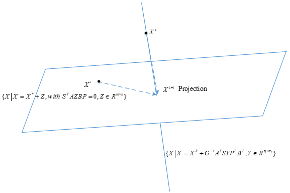
  Fig.  3.1 : The geometry of our algorithm. The next iterate, $X^{k+1}$, is obtained by projecting $X^{k}$ onto the affine space formed by intersecting $\{X|X=X^{*}+Z,\ with\ S^{\top}AZBP=0,Z\in R^{m\times n}\}$ (see (3.1)) and $\{X|X=X^{k}+G^{-1}A^{\top}SYP^{\top}B^{\top},\ Y\in R^{\tau_{1}\times\tau_{2}}\}$ (see (3.2)).

3.2 Stochastic iterative algorithm

Now we deduce the iterative scheme for the problem (1.1). Based on the Lagrangian function of the problem 3.1, we have

$$\begin{split}\mathcal{L}\left(X,Y\right)&=\frac{1}{2}\left\|X-X^{k}\right\|_{F(G)}^{2}+\left\langle Y,S^{\top}AXBP-S^{\top}CP\right\rangle\\ &=\frac{1}{2}Tr\left(\left(X-X^{k}\right)^{\top}G\left(X-X^{k}\right)\right)+Tr\left(Y^{\top}\left(S^{\top}AXBP-S^{\top}CP\right)\right),\end{split}$$ (3.3)

where $Y$ is a Lagrangian multiplier. By using 2.2, we take the gradient of $\mathcal{L}\left(X,Y\right)$ and equate its components to zero for finding the stationary matrix:

$$\nabla_{X}\mathcal{L}\left(X,Y\right)|_{X^{k+1}} = \frac{1}{2}\left(G+G^{\top}\right)\left(X^{k+1}-X^{k}\right)+A^{\top}SYP^{\top}B^{\top}=0,$$

$$\nabla_{Y}\mathcal{L}\left(X,Y\right)|_{X^{k+1}} = S^{\top}AX^{k+1}BP-S^{\top}CP=0.$$

Since $G$ is symmetric positive definite, then we have

$$S^{\top}AX^{k}BP-S^{\top}AG^{-1}A^{\top}SYP^{\top}B^{\top}BP=S^{\top}CP,$$

$$Y=\left(S^{\top}AG^{-1}A^{\top}S\right)^{{\dagger}}S^{\top}\left(AX^{k}B-C\right)P\left(P^{\top}B^{\top}BP\right)^{{\dagger}},$$

thus, the iteration form is as follows

$$\begin{split}X^{k+1}=&X^{k}-G^{-1}A^{\top}S\left(S^{\top}AG^{-1}A^{\top}S\right)^{{\dagger}}S^{\top}\left(AX^{k}B-C\right)P\left(P^{\top}B^{\top}BP\right)^{{\dagger}}P^{\top}B^{\top}.\end{split}$$ (3.4)

Let

$$Z_{1}^{\prime}=G^{-1}A^{\top}S\left(S^{\top}AG^{-1}A^{\top}S\right)^{\dagger}S^{\top}A,\ Z_{2}=BP\left(P^{\top}B^{\top}BP\right)^{\dagger}P^{\top}B^{\top},$$

the above scheme becomes

$$X^{k+1}=X^{k}-Z_{1}^{\prime}\left(X^{k}-X^{*}\right)Z_{2}.$$ (3.5)

Therefore, the sketch-and-project method is obtained.

Especially, when $\left\|X\right\|_{F(G)}^{2}=\left\|X\right\|_{F}^{2}$, i.e., the problem

$$X^{k+1}=\arg\min\limits_{X\in\mathbb{R}{{}^{m\times n}}}\frac{1}{2}\left\|X-X^{*}\right\|_{F}^{2}.$$

With a similar process, we have

$$\begin{split}X^{k+1}=&X^{k}-A^{\top}S\left(S^{\top}AA^{\top}S\right)^{{\dagger}}S^{\top}\left(AX^{k}B-C\right)P\left(P^{\top}B^{\top}BP\right)^{{\dagger}}P^{\top}B^{\top}\\ =&X^{k}-Z_{1}\left(X^{k}-X^{*}\right)Z_{2},\end{split}$$ (3.6)

where $Z_{1}=A^{\top}S\left(S^{\top}AA^{\top}S\right)^{\dagger}S^{\top}A,\ Z_{2}=BP\left(P^{\top}B^{\top}BP\right)^{\dagger}P^{\top}B^{\top}.$

Algorithm  3.1  Stochastic Iterative Method for Matrix Equations $AXB=C$

1:Input: $A\in R^{p\times m},\ B\in R^{n\times q}$, $C\in R^{p\times q}$ and the positive definite matrix $G\in\mathbb{R}^{m\times m}$

2:Initialize: arbitrary square matrix $X_{0}\in\mathbb{R}^{m\times n}$

3:for $k=1,2,\cdots,$ do

4:     Sample parameters: $P,\ S$ are distribution over random matrices;

5:     Compute $T_{1}=G^{-1}A^{\top}S\left(S^{\top}AG^{-1}A^{\top}S\right)^{\dagger}S^{\top},\ T_{2}=P\left(P^{\top}B^{\top}BP\right)^{\dagger}P^{\top}B^{\top}$

6:     $X^{k+1}=X^{k}-T_{1}(C-AX^{k}B)T_{2}$

7:end for

8:Output: last iterate $X^{k}$

Recall that $S\in\mathbb{R}^{q\times\tau_{1}},P\in\mathbb{R}^{q\times\tau_{2}}$ (with $\tau_{1},\tau_{2}$ possibly being random) and $A\in\mathbb{R}^{q\times m},B\in\mathbb{R}^{n\times q},G\in\mathbb{R}^{m\times m}$. Let us define the random quantity

$$d=rank\left((P^{\top}B^{\top})\otimes(S^{\top}A)\right),$$

and notice that $d\leq\min\left\{\tau_{1}\tau_{2},mn\right\}$, we have

$$dim\left(Range\left((BP)\otimes(G^{-1}A^{\top}S)\right)\right)=d,dim\left(Null\left((P^{\top}B^{\top})\otimes(S^{\top}A)\right)\right)=mn-d.$$

Lemma 3.1.

With respect to the geometry induced by the $\left(I\otimes G\right)$-inner product, we have that

1. $Z_{2}\otimes Z_{1}^{\prime}$ projects orthogonally onto $d$-dimensional subspace $Range\left((BP)\otimes(G^{-1}A^{\top}S)\right).$

2. $\left(I-Z_{2}\otimes Z_{1}^{\prime}\right)$ projects orthogonally onto $\left(mn-d\right)$-dimensional subspace $Null\left((P^{\top}B^{\top})\otimes(S^{\top}A)\right).$

Proof.

See Appendix A for more details. ∎

Lemma 3.2.

Let $\widetilde{Z_{1}}=GZ_{1}^{\prime}$ and $\hat{Z_{1}}=G^{-1/2}\widetilde{Z_{1}}G^{-1/2}$ . For $Z_{1},\ Z_{1}^{\prime}$, $\widetilde{Z_{1}}$, $\hat{Z_{1}}$ and $Z_{2}$ , there exist the following relations.

1. $(Z_{1}^{\prime})^{2}=Z_{1}^{\prime}$,$Z_{1}=Z_{1}^{2},\ Z_{1}^{T}=Z_{1}$ and $Z_{2}=Z_{2}^{2},\ Z_{2}^{T}=Z_{2}$.

2. $\widetilde{Z_{1}}=\widetilde{Z_{1}}G^{-1}\widetilde{Z_{1}}$, $\widetilde{Z_{1}}^{T}=\widetilde{Z_{1}}$, $\hat{Z_{1}}=\hat{Z_{1}}^{T}$ and $\hat{Z_{1}}^{2}=\hat{Z_{1}}$.

Proof.

We can verify them directly. ∎

4 Convergence analysis

Hereunder, we detail the convergence analysis for the scheme 3.1. From Lemma 3.2, it is easy to obtain the following relation.

$$\begin{split}\rho&=1-\lambda_{\min}\left(\mathbf{E}\left[Z_{2}\otimes\hat{Z_{1}}\right]\right)\\ &=1-\lambda_{\min}\left(\left(I\otimes G^{-\frac{1}{2}}\right)\mathbf{E}\left[Z_{2}\otimes\widetilde{Z_{1}}\right]\left(I\otimes G^{-\frac{1}{2}}\right)\right)\\ &=1-\lambda_{\min}\left(\left(I\otimes G^{-1}\right)\mathbf{E}\left[Z_{2}\otimes\widetilde{Z_{1}}\right]\right)\\ &=1-\lambda_{\min}\left(\mathbf{E}\left[Z_{2}\otimes Z_{1}^{\prime}\right]\right).\end{split}$$ (4.1)

Our convergence theorems depend on the above convergence rate $\rho$.

4.1 Convergence theorem

Theorem 4.1.

For every $X^{*}\in\mathbb{R}{{}^{m\times n}}$ satisfying $AX^{*}B=C$, we have

$$\mathbf{E}\left[\left\|X^{k}-X^{*}\right\|_{F(G)}^{2}\right]\leq\rho^{k}\left\|X^{0}-X^{*}\right\|_{F(G)}^{2},$$

where $\rho=1-\lambda_{\min}\left(\mathbf{E}\left[Z_{2}\otimes Z_{1}^{\prime}\right]\right)$. Therefore, the iteration sequence generated by (3.5) converges to $X^{*}$ if $0\leq\rho<1$.

Proof.

The iteration sequence (3.5) can be rewritten as a simple fixed point formula

$$X^{k+1}-X^{*}=X^{k}-X^{*}-Z_{1}^{\prime}\left(X^{k}-X^{*}\right)Z_{2}.$$ (4.2)

According to the definition of Frobenius norm, we have

$$\begin{split}\left\|X^{k+1}-X^{*}\right\|_{F(G)}^{2}=&\left\|X^{k}-X^{*}\right\|_{F(G)}^{2}-Tr\left(\left(X^{k}-X^{*}\right)^{\top}GZ_{1}^{\prime}\left(X^{k}-X^{*}\right)Z_{2}\right)\\ &-Tr\left(Z_{2}^{\top}\left(X^{k}-X^{*}\right)^{\top}(Z_{1}^{\prime})^{\top}G\left(X^{k}-X^{*}\right)\right)+\left\|Z_{1}^{\prime}\left(X^{k}-X^{*}\right)Z_{2}\right\|_{F(G)}^{2}.\end{split}$$ (4.3)

With Lemma 3.2, $Tr(MN)=Tr(NM)$ and $G^{\top}=G$, we can get

$$\begin{split}\left\|Z_{1}^{\prime}\left(X^{k}-X^{*}\right)Z_{2}\right\|_{F(G)}^{2}&=Tr\left(Z_{2}^{\top}\left(X^{k}-X^{*}\right)^{\top}Z_{1}^{\prime\top}GZ_{1}^{\prime}\left(X^{k}-X^{*}\right)Z_{2}\right)\\ &=Tr\left(Z_{2}^{\top}\left(X^{k}-X^{*}\right)^{\top}Z_{1}^{\prime\top}\widetilde{Z_{1}}\left(X^{k}-X^{*}\right)Z_{2}\right)\\ &=Tr\left(\left(X^{k}-X^{*}\right)^{\top}\widetilde{Z_{1}}\left(X^{k}-X^{*}\right)Z_{2}\right).\end{split}$$

Using the fact $Tr(M^{\top}N)=Tr(N^{\top}M)$, we have

$$Tr\left(\left(X^{k}-X^{*}\right)^{\top}GZ_{1}^{\prime}\left(X^{k}-X^{*}\right)Z_{2}\right)=Tr\left(\left(X^{k}-X^{*}\right)^{\top}\widetilde{Z_{1}}\left(X^{k}-X^{*}\right)Z_{2}\right),$$

$$\begin{split}Tr\left(Z_{2}^{\top}\left(X^{k}-X^{*}\right)^{\top}(Z_{1}^{\prime})^{\top}G\left(X^{k}-X^{*}\right)\right)=Tr\left(\left(X^{k}-X^{*}\right)^{\top}\widetilde{Z_{1}}\left(X^{k}-X^{*}\right)Z_{2}\right).\end{split}$$

Then, by substituting the above three equations into (4.3) and using the properties of Kronecker product, we can get

$$\begin{split}\left\|X^{k+1}-X^{*}\right\|_{F(G)}^{2}&=\left\|X^{k}-X^{*}\right\|_{F(G)}^{2}-\left\|Z_{1}^{\prime}\left(X^{k}-X^{*}\right)Z_{2}\right\|_{F(G)}^{2}\\ &=\left\|X^{k}-X^{*}\right\|_{F(G)}^{2}-\left\|vec\left(Z_{1}^{\prime}\left(X^{k}-X^{*}\right)Z_{2}\right)\right\|_{I\otimes G}^{2}\\ &=\left\|X^{k}-X^{*}\right\|_{F(G)}^{2}-\left\|\left(Z_{2}^{\top}\otimes Z_{1}^{\prime}\right)vec\left(X^{k}-X^{*}\right)\right\|_{I\otimes G}^{2},\end{split}$$

From $\left\|A\right\|_{F(G)}^{2}=\left\|vec\left(A\right)\right\|_{I\otimes G}^{2}$, the second equation holds.

Taking conditional expectations, we get

$$\mathbf{E}\left[\left\|X^{k+1}-X^{*}\right\|_{F(G)}^{2}\right]=\left\|X^{k}-X^{*}\right\|_{F(G)}^{2}-\mathbf{E}\left[\left\|\left(Z_{2}^{\top}\otimes Z_{1}^{\prime}\right)vec\left(X^{k}-X^{*}\right)\right\|_{I\otimes G}^{2}\right].$$ (4.4)

By Lemmas 2.1 and 3.2, it holds

$$\begin{split}&\mathbf{E}\left[\left\|\left(Z_{2}^{\top}\otimes Z_{1}^{\prime}\right)vec\left(X^{k}-X^{*}\right)\right\|_{I\otimes G}^{2}\right]\\ =&\mathbf{E}\left[vec\left(X^{k}-X^{*}\right)^{\top}\left(Z_{2}^{\top}\otimes Z_{1}^{\prime}\right)^{\top}(I\otimes G)\left(Z_{2}^{\top}\otimes Z_{1}^{\prime}\right)vec\left(X^{k}-X^{*}\right)\right]\\ =&vec\left(X^{k}-X^{*}\right)^{\top}(I\otimes G^{1/2})\mathbf{E}\left[\left(Z_{2}^{T}\otimes(G^{-1/2}\widetilde{Z_{1}}G^{-1/2})\right)\right](I\otimes G^{1/2})vec\left(X^{k}-X^{*}\right).\end{split}$$ (4.5)

With the symmetries of $Z_{2}$ and $G^{-1/2}\widetilde{Z_{1}}G^{-1/2}$ in Lemma (3.2), it results in

$$\begin{split}\mathbf{E}\left[\left\|\left(Z_{2}^{\top}\otimes Z_{1}^{\prime}\right)vec\left(X^{k}-X^{*}\right)\right\|_{I\otimes G}^{2}\right]&\geq\lambda_{\min}\left(\mathbf{E}\left[Z_{2}^{\top}\otimes\hat{Z_{1}}\right]\right)\left\|(I\otimes G^{1/2})vec\left(X^{k}-X^{*}\right)\right\|_{2}^{2}\\ &=\rho_{c}\left\|X^{k}-X^{*}\right\|_{F(G)}^{2},\end{split}$$ (4.6)

where $\left\|(I\otimes G^{1/2})vec\left(X^{k}-X^{*}\right)\right\|_{2}^{2}=\left\|vec\left(X^{k}-X^{*}\right)\right\|_{F(G)}^{2}$ and $\rho_{c}=\lambda_{\min}\left(\mathbf{E}\left[Z_{2}^{\top}\otimes\hat{Z_{1}}\right]\right)$. For the inequality, the following estimate $\lambda_{\min}=\underset{x\neq 0}{\min}\dfrac{x^{\top}Ax}{x^{\top}x}$ is used.

Therefore, combining (4.4) and (4.6), we can obtain an estimate as follows

$$\mathrm{E}\left[\left\|X^{k+1}-X^{*}\right\|_{F(G)}^{2}\right]=\left(1-\rho_{c}\right)\left\|X^{k}-X^{*}\right\|_{F(G)}^{2}.$$

Taking the full expectation of both sides, we can get that

$$\mathbf{E}\left[\left\|X^{k+1}-X^{*}\right\|_{F(G)}^{2}\right]=\left(1-\rho_{c}\right)\mathbf{E}\left[\left\|X^{k}-X^{*}\right\|_{F(G)}^{2}\right].$$

By induction on the above process, the proof is completed. ∎

Theorem 4.2.

For every $X^{*}\in\mathbb{R}{{}^{m\times n}}$ satisfying $AX^{*}B=C$, we have the norm of expectation as follows

$$\left\|\mathbf{E}\left[X^{k+1}-X^{*}\right]\right\|_{F(G)}\leq\rho^{k}\left\|X^{0}-X^{*}\right\|_{F(G)},$$

where $\rho=\lambda_{\max}\left(I-\mathbf{E}\left[Z_{2}\otimes Z_{1}^{\prime}\right]\right)=1-\lambda_{\min}(\mathbf{E}\left[Z_{2}\otimes Z_{1}^{\prime}\right])$.

Proof.

By the Kronecker product, the iterative formula (3.5) can be written as follows

$$vec\left(X^{k+1}-X^{*}\right)=\left(I-\left(Z_{2}^{\top}\otimes Z_{1}^{\prime}\right)\right)vec\left(X^{k}-X^{*}\right).$$ (4.7)

It is evident that the transform $X\rightarrow vec\left(X\right)$ gives a linear isomorph of $\mathbb{R}{{}^{m\times n}}\rightarrow\mathbb{R}{{}^{mn}}$. Since $Z_{2}^{\top}=Z_{2}$, taking expectations conditioned on $X^{k}$ in (4.7) we have

$$\mathbf{E}\left[vec\left(X^{k+1}-X^{*}\right)|vec\left(X^{k}\right)\right]=\left(I-\mathbf{E}\left[Z_{2}\otimes Z_{1}^{\prime}\right]\right)vec\left(X^{k}-X^{*}\right).$$

Taking expectations again gives

$$\mathbf{E}\left[vec\left(X^{k+1}-X^{*}\right)\right]=\left(I-\mathbf{E}\left[Z_{2}\otimes Z_{1}^{\prime}\right]\right)\mathbf{E}\left[vec\left(X^{k}-X^{*}\right)\right].$$

Applying Lemma 3.2 and the norms to both sides we obtain the estimate

$$\begin{split}\left\|\mathbf{E}\left[vec\left(X^{k+1}-X^{*}\right)\right]\right\|^{2}_{I\otimes G}&=\left\|\left(I-\mathbf{E}\left[Z_{2}\otimes Z_{1}^{\prime}\right]\right)\mathbf{E}\left[vec\left(X^{k}-X^{*}\right)\right]\right\|^{2}_{I\otimes G}\\ &\leq\left\|\left(I-\mathbf{E}\left[Z_{2}\otimes Z_{1}^{\prime}\right]\right)\right\|^{2}_{I\otimes G}\left\|\mathbf{E}\left[vec\left(X^{k}-X^{*}\right)\right]\right\|^{2}_{I\otimes G}\end{split}$$

$$\begin{split}\left\|\left(I-\mathbf{E}\left[Z_{2}\otimes Z_{1}^{\prime}\right]\right)\right\|^{2}_{I\otimes G}&=\underset{\left\|(I\otimes G^{1/2})x\right\|_{2}=1}{\max}\left\|(I\otimes G^{1/2})\left(I-\mathbf{E}\left[Z_{2}\otimes Z_{1}^{\prime}\right]\right)x\right\|^{2}_{2}.\end{split}$$

Substituting $y=G^{1/2}x$ in the above gives

$$\begin{split}\left\|\left(I-\mathbf{E}\left[Z_{2}\otimes Z_{1}^{\prime}\right]\right)\right\|^{2}_{I\otimes G}&=\underset{\left\|y\right\|_{2}=1}{\max}\left\|(I\otimes G^{1/2})\left(I-\mathbf{E}\left[Z_{2}\otimes Z_{1}^{\prime}\right]\right)(I\otimes G^{-1/2})y\right\|^{2}_{2}\\ &=\underset{\left\|y\right\|_{2}=1}{\max}\left\|\left(I-\mathbf{E}\left[Z_{2}\otimes(G^{-1/2}\widetilde{Z_{1}}G^{-1/2})\right]\right)y\right\|^{2}_{2}\\ &=\lambda_{\max}^{2}\left(I-\mathbf{E}\left[Z_{2}\otimes(G^{-1/2}\widetilde{Z_{1}}G^{-1/2})\right]\right),\end{split}$$

the third equality we used the symmetry of $I-\mathbf{E}\left[Z_{2}\otimes(G^{-1/2}\widetilde{Z_{1}}G^{-1/2})\right]$ when passing from the operator norm to the spectral radius. Note that the symmetry of $\mathbf{E}\left[Z_{2}\otimes(G^{-1/2}\widetilde{Z_{1}}G^{-1/2})\right]$ derives from the symmetries of $Z_{2}$ and $G^{-1/2}\widetilde{Z_{1}}G^{-1/2}$ in Lemma 3.2. Considering that the vector operator is isomorphic and $\left\|vec(X^{k}-X^{*})\right\|^{2}_{I\otimes G}=\left\|X^{k}-X^{*}\right\|^{2}_{F(G)}$, with the formula (4.1) we have

$$\begin{split}\left\|\mathbf{E}\left[X^{k+1}-X^{*}\right]\right\|_{F(G)}&=\left\|\mathbf{E}\left[vec\left(X^{k+1}-X^{*}\right)\right]\right\|_{I\otimes G}\\ &\leq\rho\left\|\mathbf{E}\left[X^{k}-X^{*}\right]\right\|_{F(G)}.\end{split}$$

By induction, the conclusion follows. The proof is completed. ∎

4.2 Convergence rate and convergence conditions

To show that the rate $\rho$ is meaningful, in Lemma 4.3 we prove that $0\leq\rho\leq 1$. We also provide a meaningful lower bound for $\rho$.

Theorem 4.3.

The quantity $\rho=1-\lambda_{\min}\left(Z_{2}\otimes Z_{1}^{\prime}\right)$ satisfies

$$0\leq 1-\frac{\mathbf{E}\left[d\right]}{mn}\leq\rho\leq 1,$$

where $d=rank\left((P^{\top}B^{\top})\otimes(S^{\top}A)\right)$.

Proof.

Through Lemma 3.2 we known $Z_{2}\otimes\hat{Z_{1}}$ is a projection, then we get

$$\left[\left(I\otimes G^{-1/2}\right)\left(Z_{2}\otimes\widetilde{Z_{1}}\right)\left(I\otimes G^{-1/2}\right)\right]^{2}=\left(I\otimes G^{-1/2}\right)\left(Z_{2}\otimes\widetilde{Z_{1}}\right)\left(I\otimes G^{-1/2}\right),$$

where$\widetilde{Z_{1}}=GZ_{1}$, whence the spectrum of $\left(I\otimes G^{-1/2}\right)\left(Z_{2}\otimes\widetilde{Z_{1}}\right)\left(I\otimes G^{-1/2}\right)$ is contained in $\left\{0,1\right\}$. Using this, combined with the fact that the mapping $A\rightarrow\lambda_{\max}\left(A\right)$ is convex on the set of symmetric matrices and Jensen’s inequality, we have

$$\begin{split}\lambda_{\max}\left(\mathbf{E}\left[Z_{2}\otimes Z_{1}^{\prime}\right]\right)&=\lambda_{\max}\left(\left(I\otimes G^{-1/2}\right)\mathbf{E}\left[Z_{2}\otimes\widetilde{Z_{1}}\right]\left(I\otimes G^{-1/2}\right)\right)\\ &\leq\mathbf{E}\left[\lambda_{\max}\left(Z_{2}\otimes G^{-1/2}\widetilde{Z_{1}}G^{-1/2}\right)\right]\leq 1.\end{split}$$

Analogously, with the convexity of the mapping $A\rightarrow-\lambda_{\min}\left(A\right)$, it holds $\lambda_{\min}\left(\mathbf{E}\left[Z_{2}\otimes Z_{1}^{\prime}\right]\right)\geq 0$. Thus $\lambda_{\min}\left(\mathbf{E}\left[Z_{2}\otimes Z_{1}^{\prime}\right]\right)\in\left[0,1\right]$ which implies $0\leq\rho\leq 1$. To the lower bound, we use the fact that the trace of a matrix is the sum of its eigenvalues, and have

$$\mathbf{E}\left[Tr\left(Z_{2}\otimes Z_{1}^{\prime}\right)\right]=Tr\left(\mathbf{E}\left[Z_{2}\otimes Z_{1}^{\prime}\right]\right)\geq mn\lambda_{\min}\left(\mathbf{E}\left[Z_{2}\otimes Z_{1}^{\prime}\right]\right).$$

Since $Z_{2}\otimes Z_{1}^{\prime}$ is project on a d-dimensional subspace from Lemma 3.1, it results in $Tr\left(Z_{2}\otimes Z_{1}^{\prime}\right)=d$. Thus, from the above formula, we can get

$$\rho=1-\lambda_{\min}\left(\mathbf{E}\left[Z_{2}\otimes Z_{1}^{\prime}\right]\right)\geq 1-\frac{\mathbf{E}\left[d\right]}{mn}.$$

∎

Lemma 4.1.

If $\mathbf{E}\left[Z_{2}\otimes\widetilde{Z_{1}}\right]$ is invertible, then $\rho=1-\lambda_{min}\left(\mathbf{E}\left[Z_{2}\otimes Z_{1}^{\prime}\right]\right)<1$, $B^{\top}\otimes A$ and $(BP)^{\top}\otimes(S^{\top}A)$ have full column rank, and $X^{*}$ is unique.

Proof.

See Appendix for more details. ∎

Lemma 4.2 ([17]).

If $A\in\mathbb{R}^{n\times n}$ is symmetric positive definite and $X\in\mathbb{R}^{n\times k}$ has rank $k$, then $B=X^{\top}AX\in\mathbb{R}^{k\times k}$ is also symmetric positive definite.

Lemma 4.3.

For an arbitrary symmetric positive definite matrix $A$, there exists $\mathbf{E}\left[A^{2}\right]\succeq\left(\mathbf{E}\left[A\right]\right)^{\top}\mathbf{E}\left[A\right].$

Proof.

See Appendix for more details. ∎

Lemma 4.4.

$(BP)^{\top}\otimes(S^{\top}A)$ is full column rank if and only if $\mathbf{E}\left[Z_{2}\otimes\widetilde{Z_{1}}\right]$ is symmetric positive definite .

Proof.

Since $(BP)^{\top}\otimes(S^{\top}A)$ is full column rank and $G$ is symmetric positive definite, we can get $Z_{2}\otimes\widetilde{Z_{1}}$ is symmetric positive definite by Lemma 4.2. Since $Z_{2}\otimes\widetilde{Z_{1}}$ is symmetric positive definite, it holds $Z_{2}^{\top}\otimes\widetilde{Z_{1}}=H^{\top}H$ where $H$ is symmetric positive definite. Then, for every $y\in\mathbb{R}^{mn}\neq 0$,

$$\begin{split}y^{\top}\mathbf{E}\left[\left(Z_{2}^{\top}\otimes\widetilde{Z_{1}}\right)\right]y&=y^{\top}\mathbf{E}\left[H^{\top}H\right]y\\ &\geq y^{\top}\mathbf{E}\left[H\right]^{\top}\mathbf{E}\left[H\right]y\\ &>0.\end{split}$$

The first inequality is obtained by Lemma 4.3. It is easy to know that $y^{\top}\mathbf{E}\left[H\right]^{\top}\mathbf{E}\left[H\right]y\geq 0$. If $y^{\top}\mathbf{E}\left[H\right]^{\top}\mathbf{E}\left[H\right]y=0,$ then $y^{\top}\mathbf{E}\left[H\right]y=0$, i.e., $y^{\top}Hy=0$ which contradicts with the property that $H$ is symmetric positive definite. Thus, the necessity exists. Meanwhile, the sufficiency is obtained by Lemma 4.1. ∎

Lemma 4.5 ([14]).

Let $Z=Z_{2}\otimes\widetilde{Z_{1}}$. If $\mathbf{E}\left[Z\right]$ is symmetric positive definite, then

$$\left\langle\mathbf{E}\left[Z\right]y,y\right\rangle\geq\left(1-\rho\right)\left\|y\right\|^{2}_{I\otimes G},\ \ \text{for all\ }y\in\mathbb{R}^{mn},$$

where $\rho=1-\lambda_{\min}\left(Z_{2}\otimes Z_{1}^{\prime}\right)$ and $G$ symmetric positive definite.

Proof.

Note that $\mathbf{E}\left[Z_{2}\otimes\widetilde{Z_{1}}\right]$ and $G$ are symmetric positive definite, we get

$$\begin{split}1-\rho&=1-\lambda_{\min}\left(\left(I\otimes G^{-\frac{1}{2}}\right)\mathbf{E}\left[Z_{2}\otimes\widetilde{Z_{1}}\right]\left(I\otimes G^{-\frac{1}{2}}\right)\right)\\ &=\underset{t}{max}\left\{t|\left(I\otimes G^{-\frac{1}{2}}\right)\mathbf{E}\left[Z_{2}\otimes\widetilde{Z_{1}}\right]\left(I\otimes G^{-\frac{1}{2}}\right)-tI\succeq 0\right\}\\ &=\underset{t}{max}\left\{t|\mathbf{E}\left[Z_{2}\otimes\widetilde{Z_{1}}\right]-t(I\otimes G)\succeq 0\right\}.\\ \end{split}$$

Therefore, $\mathbf{E}\left[Z_{2}\otimes\widetilde{Z_{1}}\right]\succeq I\otimes G$, and the conclusion is obtained. ∎

Theorem 4.4.

If $(BP)^{\top}\otimes(S^{\top}A)$ is full column rank, then

$$\mathbf{E}\left[\left\|X^{k}-X^{*}\right\|^{2}_{F(G)}\right]\leq\rho^{k}\left\|X^{0}-X^{*}\right\|^{2}_{F(G)},$$

where $\rho<1$ is given in Lemma 4.1.

Proof.

Since $(BP)^{\top}\otimes(S^{\top}A)$ is full column rank, from Lemma 4.4 we know that $\mathbf{E}\left[Z_{2}\otimes\widetilde{Z_{1}}\right]$ is symmetric positive definite. Let $r^{k}=vec\left(X^{k}-X^{*}\right)$. From (3.5) we have $r^{k+1}=r^{k}-\left(Z_{2}^{\top}\otimes Z_{1}^{\prime}\right)r^{k}$. Taking expectation in $\left\|r^{k+1}\right\|^{2}_{I\otimes G}$ conditioned on $r^{k}$ gives

$$\begin{split}\mathbf{E}\left[\left\|r^{k+1}\right\|^{2}_{I\otimes G}|r^{k}\right]&=\mathbf{E}\left[\left\|\left(I-Z^{\top}_{2}\otimes Z_{1}^{\prime}\right)r^{k}\right\|^{2}_{I\otimes G}|r^{k}\right]\\ &=\mathbf{E}\left[\left\langle\left[\left(I\otimes G\right)-\left(Z_{2}^{\top}\otimes GZ_{1}^{\prime}\right)\right]r^{k},r^{k}\right\rangle|r^{k}\right]\\ &=\left\|r^{k}\right\|^{2}_{I\otimes G}-\left\langle\mathbf{E}\left[Z_{2}^{\top}\otimes\widetilde{Z_{1}}\right]r^{k},r^{k}\right\rangle\\ &\leq\rho\left\|r^{k}\right\|^{2}_{I\otimes G}\ \ \left(by\ Lemma\ \ref{lem:7.4}\right).\end{split}$$

Since $\left\|r^{k}\right\|^{2}_{I\otimes G}=\left\|X^{k}-X^{*}\right\|^{2}_{F(G)}$, then the conclusion follows.

∎

Remark 4.1.

When $A$ is full column rank or $x\in Range(A^{\top})$, the following estimate holds $\left\|Ax\right\|_{2}^{2}\geq\sigma_{\min}^{2}(A)\|x\|_{2}^{2}.$ For one case of the matrix with full column rank, 4.5 give the convergence of the generalized method. For the other case, some conclusions are given in the following. For special methods, some results have been obtained (for the GRBK method, see [10]).

Lemma 4.6 ([12]).

Let $A\in\mathbb{R}^{p\times m}$ and $B\in\mathbb{R}^{n\times q}$ be given. Denote

$$\mathcal{M}=\left\{M\in\mathbb{R}^{m\times n}|\exists Y\in\mathbb{R}^{p\times q}\ s.t.\ M=A^{\top}YB^{\top}\right\}.$$ (4.8)

Then, for any matrix $M\in\mathcal{M}$, it holds

$$\left\|AMB\right\|^{2}_{F}\geq\sigma_{\min}^{2}\left(A\right)\sigma_{\min}^{2}\left(B\right)\left\|M\right\|^{2}_{F}.$$

Lemma 4.7.

Let the two sets $M_{1}$ and $M_{2}$ be defined by

$$M_{1}=\left\{X_{1}\in\mathbf{R}^{m\times n}|A^{\top}Y_{1}B^{\top}=X_{1}\ \text{ for some }Y_{1}\in\mathbf{R}^{p\times q}\right\},M_{2}=\left\{X_{2}\in\mathbf{R}^{m\times n}|A^{\top}AY_{2}BB^{\top}=X_{2}\ \text{ for some }Y_{2}\in\mathbf{R}^{m\times n}\right\}.$$

Then, it holds $M_{1}=M_{2}$.

Proof.

See Appendix for more details. ∎

Theorem 4.5.

Assume that $Z_{1}^{\prime}$ and $Z_{2}$ are independent random variables. Let

$$\mathcal{\bar{M}}=\left\{\bar{M}\in\mathbb{R}^{m\times n}|\exists Y\in\mathbb{R}^{p\times q}\ s.t.\ \bar{M}=\mathbf{E}\left[Z_{1}^{\prime}\right]Y\mathbf{E}\left[Z_{2}\right]\right\}.$$

If $(X^{k}-X^{*})\in\mathcal{\bar{M}},$ then for every $X^{*}\in\mathbb{R}{{}^{m\times n}}$ satisfying $AX^{*}B=C$, we have

$$\mathbf{E}\left[\left\|X^{k}-X^{*}\right\|_{F(G)}^{2}\right]\leq\rho_{\sigma}^{k}\left\|X^{0}-X^{*}\right\|_{F(G)}^{2}.$$

with $\rho_{\sigma}=1-\sigma^{2}_{\min}\left(\mathbf{E}\left[Z_{2}\otimes Z_{1}^{\prime}\right]\right)<1$. Therefore, the iteration sequence generated by (3.6) converges to $X^{*}$.

Proof.

From Lemma 3.2, we can get $Z_{2}^{T}\otimes\hat{Z_{1}}=\left(Z_{2}^{T}\otimes\hat{Z_{1}}\right)^{T}$, $\left(Z_{2}^{T}\otimes\hat{Z_{1}}\right)^{2}=Z_{2}^{T}\otimes\hat{Z_{1}}$ . Thus, for every $y\in R^{mn}$, we have

$$\begin{split}y^{T}\mathbf{E}\left[\left(Z_{2}^{T}\otimes\hat{Z_{1}}\right)\right]y&=y^{T}\mathbf{E}\left[\left(Z_{2}^{T}\otimes\hat{Z_{1}}\right)^{\top}\left(Z_{2}^{T}\otimes\hat{Z_{1}}\right)\right]y\\ &\geq y^{T}\mathbf{E}\left[\left(Z_{2}^{T}\otimes\hat{Z_{1}}\right)\right]^{\top}\mathbf{E}\left[\left(Z_{2}^{T}\otimes\hat{Z_{1}}\right)\right]y.\end{split}$$

Using (4.5), we can get

$$\begin{split}\mathbf{E}\left[\left\|\left(Z_{2}^{\top}\otimes Z_{1}^{\prime}\right)\text{vec}\left(X^{k}-X^{*}\right)\right\|_{I\otimes G}^{2}\right]&\geq\left\|\mathbf{E}\left[\left(Z_{2}^{T}\otimes\hat{Z_{1}}\right)\right](I\otimes G^{1/2})\text{vec}\left(X^{k}-X^{*}\right)\right\|_{2}^{2}\\ &=\left\|\mathbf{E}\left[\hat{Z_{1}}\right]\hat{R^{k}}\mathbf{E}\left[Z_{2}\right]\right\|_{F}^{2}\\ &\geq\sigma_{\min}^{2}\left(\mathbf{E}\left[Z_{2}\right]\right)\sigma_{\min}^{2}\left(\mathbf{E}\left[\hat{Z_{1}}\right]\right)\left\|\hat{R^{k}}\right\|_{F}^{2}\\ &=\sigma^{2}_{\min}\left(\mathbf{E}\left[Z_{2}\otimes Z_{1}^{\prime}\right]\right)\left\|X^{k}-X^{*}\right\|_{F(G)}^{2},\end{split}$$ (4.9)

where $\hat{R^{k}}=G^{1/2}(X^{k}-X^{*})$. The first inequality is obtained by $\mathbf{E}\left[\left\|X-\mathbf{E}\left[X\right]\right\|^{2}\right]=\mathbf{E}\left[\left\|X\right\|^{2}\right]-\left\|\mathbf{E}\left[X\right]\right\|^{2}$. From $(X^{k}-X^{*})\in\mathcal{\bar{M}}$, $\hat{Z_{1}}=\hat{Z_{1}}^{T}$ and $Z_{2}^{T}=Z_{2}$, it yields

$$\hat{R^{k}}\in\mathcal{\hat{M}}=\left\{\hat{M}\in\mathbb{R}^{m\times n}|\exists Y\in\mathbb{R}^{p\times q}\ s.t.\ \hat{M}=\mathbf{E}\left[\hat{Z}_{1}\right]^{T}Y\mathbf{E}\left[(Z_{2})\right]^{T}\right\}.$$

It is easy to know that $vec(\hat{R^{k}})=(I\otimes G^{1/2})\text{vec}\left(X^{k}-X^{*}\right)$, $\left\|\hat{R^{k}}\right\|_{F}^{2}=\left\|X^{k}-X^{*}\right\|_{F(G)}^{2}$. Then, with the use of Lemma 4.6 the second inequality holds. Since $\sigma_{\min}\left(\mathbf{E}\left[\hat{Z}_{1}\right]\right)=\sigma_{\min}\left(\mathbf{E}\left[Z_{1}^{\prime}\right]\right)$, we have $\sigma_{\min}^{2}\left(\mathbf{E}\left[Z_{2}\right]\right)\sigma_{\min}^{2}\left(\mathbf{E}\left[\hat{Z_{1}}\right]\right)=\sigma^{2}_{\min}\left(\mathbf{E}\left[Z_{2}\otimes Z_{1}^{\prime}\right]\right).$ With the similar process of Theorem 4.1, the conclusion is obtained. ∎

Remark 4.2.

It is easy to prove that $(X^{k}-X^{*})\in\mathcal{\bar{M}}$ is equivalent to $(I\otimes G^{1/2})\text{vec}\left(X^{k}-X^{*}\right)\in Range\left(\mathbf{E}\left[\left(Z_{2}^{T}\otimes\hat{Z_{1}}\right)\right]\right)$. In the global randomized Kaczmarz method, $\mathbf{E}\left[Z_{1}^{\prime}\right]=\mathbf{E}\left[\hat{Z}_{1}\right]=\frac{A^{\top}A}{\left\|A\right\|^{2}_{F}}$, $\mathbf{E}\left[Z_{2}\right]=\frac{BB^{T}}{\left\|B\right\|^{2}_{F}}$, it has

$$\mathcal{\bar{M}}=\left\{\bar{M}\in\mathbb{R}^{m\times n}|\exists Y\in\mathbb{R}^{p\times q}\ s.t.\ \bar{M}=A^{T}AYBB^{T}\right\}.$$

Obviously, $\mathcal{\bar{M}}$ is well defined because $X^{0}=O\in\mathcal{\bar{M}}$ and $A^{\dagger}CB^{\dagger}\in\mathcal{\bar{M}}$. Meanwhile, it is easy to verify that $(X^{k}-X^{*})\in\mathcal{M}$ in (4.8) with the iteration scheme (3.6) for the global randomized Kaczmarz method. Then it results in $(X^{k}-X^{*})\in\mathcal{\bar{M}}$ from Lemma 4.7.

4.3 Convergence with convenient probabilities

Definition 4.6 ([14]).

Let the random matrix $S,P$ be discrete distributions. $(S,P)$ will be called a complete discrete sampling pair if $S=S_{i}\in\mathbb{R}^{p\times\tau_{1i}}$ with probability $p^{1}_{i}>0$, where $S_{i}^{\top}A$ has full row rank and $\tau_{1i}\in\mathbb{N}$ for $i=1,...,r_{1}$. ${\bf S}=:\left[S_{1},...,S_{r_{1}}\right]\in\mathbb{R}^{p\times\Sigma^{r_{1}}_{i=1}\tau_{1i}}$ is such that $A^{\top}{\bf S}$ has full row rank. Meanwhile, $P=P_{i}\in\mathbb{R}^{q\times\tau_{2i}}$ with probability $p^{2}_{i}>0$, where $P_{i}^{\top}B^{\top}$ has full row rank and $\tau_{2i}\in\mathbb{N}$ for $i=1,...,r_{2}$. ${\bf P}=:\left[P_{1},...,P_{r_{2}}\right]\in\mathbb{R}^{q\times\Sigma^{r_{2}}_{i=1}\tau_{2i}}$ is such that $B{\bf P}$ has full row rank.

Assume that $S,P$ is a complete discrete sampling pair, then $S^{\top}A$ and $(BP)^{\top}$ have full row rank and

$$\left(S^{\top}AA^{\top}S\right)^{\dagger} = \left(S^{\top}AA^{\top}S\right)^{-1},$$

$$\left(P^{\top}B^{\top}BP\right)^{\dagger} = \left(P^{\top}B^{\top}BP\right)^{-1}.$$

Therefore we replace the pseudoinverse in (3.6) by the inverse. Define

$$D_{S}=\text{diag}\left(\sqrt{p^{1}_{1}}\left(\left(S_{1}\right)^{\top}AA^{\top}S_{1}\right)^{-1/2},...,\sqrt{p^{1}_{r_{1}}}\left(\left(S_{r_{1}}\right)^{\top}AA^{\top}S_{r_{1}}\right)^{-1/2}\right),$$ (4.10)

$$D_{P}=\text{diag}\left(\sqrt{p^{2}_{1}}\left(\left(P_{1}\right)^{\top}B^{\top}BP_{1}\right)^{-1/2},\ ...\ ,\sqrt{p^{2}_{r_{2}}}\left(\left(P_{r_{2}}\right)^{\top}B^{\top}BP_{r_{2}}\right)^{-1/2}\right),$$ (4.11)

where $D_{S}$ and $D_{P}$ are block diagonal matrices, and are well defined and invertible, as $S_{i}^{\top}A$ has full row rank for $i=1,...,r_{1}$ and $P_{j}^{\top}B^{\top}$ has full row rank for $j=1,...,r_{2}$. Taking the expectation of $Z_{1}$ and $Z_{2}$, we get

$$\begin{split}\mathbf{E}\left[Z_{1}\right]&=\sum\limits_{i=1}^{r_{1}}A^{\top}S_{i}\left(S_{i}^{\top}AA^{\top}S_{i}\right)^{-1}S_{i}^{\top}Ap^{1}_{i}\\ &=A^{\top}\left(\sum\limits_{i=1}^{r_{1}}S_{i}\sqrt{p^{1}_{i}}\left(S_{i}^{\top}AA^{\top}S_{i}\right)^{-1/2}\left(S_{i}^{\top}AA^{\top}S_{i}\right)^{-1/2}\sqrt{p^{1}_{i}}S_{i}^{\top}\right)A\\ &=\left(A^{\top}{\bf S}D_{S}\right)\left(D_{S}{\bf S^{\top}}A\right),\end{split}$$ (4.12)

and

$$\begin{split}\mathbf{E}\left[Z_{2}\right]&=\sum\limits_{j=1}^{r_{2}}BP_{j}\left(P_{j}^{\top}B^{\top}BP_{j}\right)^{-1}P_{j}^{\top}B^{\top}p^{2}_{j}\\ &=B\left(\sum\limits_{j=1}^{r_{2}}P_{j}\sqrt{p^{2}_{j}}\left(P_{j}^{\top}B^{\top}BP_{j}\right)^{-1/2}\left(P_{j}^{\top}B^{\top}BP_{j}\right)^{-1/2}\sqrt{p^{2}_{j}}P_{j}^{\top}\right)B^{\top}\\ &=\left(B{\bf P}D_{P}\right)\left(D_{P}{\bf P}^{\top}B^{\top}\right).\end{split}$$ (4.13)

Since $A^{\top}{\bf S}$ and $B{\bf P}$ have full row rank, and $D_{S},\ D_{P}$ are invertible, we can get $\mathbf{E}\left[Z_{i}\right],i=1,2$ are symmetric positive definite. So, complete discrete sampling pairs guarantee the convergence of the resulting methods.

Next we develop a choice of probability distribution that yields a convergence rate that is easy to interpret. This result is new and covers a wide range of methods, including randomized Kaczmarz method and randomized coordinate descent method, as well as their block variants. However, it is more general and covers many other possible particular algorithms, which arise by choosing two particular sets of sample matrices $S_{i}$ for $i=1,...,r_{1}$ and $P_{j}$ for $j=1,...,r_{2}$.

Theorem 4.7.

Assume that $(S,P)$ is a complete discrete sampling pair with the following probabilities, respectively,

$$p^{1}_{i}=\frac{Tr\left(S_{i}^{\top}AA^{\top}S_{i}\right)}{\left\|A^{\top}{\bf S}\right\|^{2}_{F}}\ \ \text{for}\ \ i=1,...,r_{1},\ p^{2}_{j}=\frac{Tr\left(P_{j}^{\top}B^{\top}BP_{j}\right)}{\left\|B{\bf P}\right\|^{2}_{F}}\ \ \text{for}\ \ j=1,...,r_{2},$$ (4.14)

Then the formula (3.6) satisfies

$$\mathbf{E}\left[\left\|X^{k}-X^{*}\right\|^{2}_{F}\right]\leq\rho^{k}\left\|X^{0}-X^{*}\right\|^{2}_{F},$$ (4.15)

where

$$\rho=1-\frac{\lambda_{\min}\left({\bf S}^{\top}AA^{\top}{\bf S}\right)\lambda_{\min}\left({\bf P}^{\top}B^{\top}B{\bf P}\right)}{\left\|A^{\top}{\bf S}\right\|^{2}_{F}\left\|B{\bf P}\right\|^{2}_{F}}.$$ (4.16)

Proof.

Let $u_{i}=Tr\left(\left(S_{i}\right)^{\top}AA^{\top}S_{i}\right)$, $v_{j}=Tr\left(\left(P_{j}\right)^{\top}B^{\top}BP_{j}\right)$. Taking (4.14) into (4.10) and (4.11), respectively, we have

$$D_{S}^{2} = \frac{1}{\left\|A^{\top}S\right\|_{F}^{2}}\text{diag}\left(u_{1}\left(S_{1}^{\top}AA^{\top}S_{1}\right)^{-1},...,u_{r_{1}}\left(S_{r_{1}}^{\top}AA^{\top}S_{r_{1}}\right)^{-1}\right),$$

$$D_{P}^{2} = \frac{1}{\left\|BP\right\|_{F}^{2}}\text{diag}\left(v_{1}\left(P_{1}^{\top}B^{\top}BP_{1}\right)^{-1},...,v_{r_{2}}\left(P_{r_{2}}^{\top}B^{\top}BP_{r_{2}}\right)^{-1}\right).$$

and thus

$$\lambda_{\min}\left(D_{S}^{2}\right) = \frac{1}{\left\|A^{\top}{\bf S}\right\|_{F}^{2}}\min\limits_{1\leq i\leq r_{1}}\left\{\frac{u_{i}}{\lambda_{\max}\left(S_{i}^{\top}AA^{\top}S_{i}\right)}\right\}\geq\frac{1}{\left\|A^{\top}{\bf S}\right\|_{F}^{2}},$$ (4.17)

$$\lambda_{\min}\left(D_{P}^{2}\right) = \frac{1}{\left\|B{\bf P}\right\|_{F}^{2}}\min\limits_{1\leq j\leq r_{2}}\left\{\frac{v_{j}}{\lambda_{\max}\left(P_{j}^{\top}B^{\top}BP_{j}\right)}\right\}\geq\frac{1}{\left\|B{\bf P}\right\|_{F}^{2}}.$$ (4.18)

Using the fact that for arbitrary matrices $M$, $N$ of appropriate sizes, $\lambda_{\min}\left(MN\right)=\lambda_{\min}\left(NM\right)$, hence

$$\begin{split}\lambda_{\min}\left(\mathbf{E}\left[Z_{1}\right]\right)&=\lambda_{\min}\left(A^{\top}{\bf S}D_{S}^{2}{\bf S}^{\top}A\right)\\ &=\lambda_{\min}\left({\bf S}^{\top}AA^{\top}{\bf S}D_{S}^{2}\right).\end{split}$$

Then, using the fact that $\lambda_{\min}\left(MN\right)=\lambda_{\min}\left(M\right)\lambda_{\min}\left(N\right)$ for $M,N\in\mathbb{R}^{n\times n}$ are symmetric positive definite, from (4.17) we can obtain

$$\begin{split}\lambda_{\min}\left(\mathbf{E}\left[Z_{1}\right]\right)&=\lambda_{\min}\left({\bf S}^{\top}AA^{\top}{\bf S}D_{S}^{2}\right)\\ &\geq\lambda_{\min}\left({\bf S}^{\top}AA^{\top}{\bf S}\right)\lambda_{\min}\left(D_{S}^{2}\right)\\ &\geq\frac{\lambda_{\min}\left({\bf S}^{\top}AA^{\top}{\bf S}\right)}{\left\|A^{\top}{\bf S}\right\|_{F}^{2}}.\end{split}$$

Similarly, we can also obtain

$$\begin{split}\lambda_{\min}\left(\mathbf{E}\left[Z_{2}\right]\right)&=\lambda_{\min}\left(B{\bf P}D_{P}^{2}{\bf P}^{\top}B^{\top}\right)\\ &=\lambda_{\min}\left({\bf P}^{\top}B^{\top}B{\bf P}D_{P}^{2}\right)\\ &\geq\lambda_{\min}\left({\bf P}^{\top}B^{\top}B{\bf P}\right)\lambda_{\min}\left(D_{P}^{2}\right)\\ &\geq\frac{\lambda_{\min}\left({\bf P}^{\top}B^{\top}B{\bf P}\right)}{\left\|B{\bf P}\right\|_{F}^{2}}.\end{split}$$

Since

$$\begin{split}\rho_{c}&=\lambda_{\min}\left(\mathbf{E}\left[Z_{2}^{\top}\otimes Z_{1}\right]\right)\\ &=\lambda_{\min}\left(\mathbf{E}\left[Z_{2}^{\top}\right]\otimes\mathbf{E}\left[Z_{1}\right]\right)\\ &\geq\lambda_{\min}\left(\mathbf{E}\left[Z_{2}\right]\right)\lambda_{\min}\left(\mathbf{E}\left[Z_{1}\right]\right)\\ &\geq\frac{\lambda_{\min}\left({\bf S}^{\top}AA^{\top}{\bf S}\right)\lambda_{\min}\left({\bf P}^{\top}B^{\top}B{\bf P}\right)}{\left\|A^{\top}{\bf S}\right\|_{F}^{2}\left\|B{\bf P}\right\|_{F}^{2}}.\end{split}$$

Hence, by Theorem 4.1 we have

$$\begin{split}\mathbf{E}\left[\left\|X^{k}-X^{*}\right\|^{2}_{F}\right]&\leq\left(1-\rho_{c}\right)\left\|X^{k-1}-X^{*}\right\|^{2}_{F}\\ &\leq\left(1-\frac{\lambda_{\min}\left({\bf S}^{\top}AA^{\top}{\bf S}\right)\lambda_{\min}\left({\bf P}^{\top}B^{\top}B{\bf P}\right)}{\left\|A^{\top}{\bf S}\right\|_{F}^{2}\left\|B{\bf P}\right\|_{F}^{2}}\right)\left\|X^{k-1}-X^{*}\right\|^{2}_{F}\\ &=\rho\left\|X^{k-1}-X^{*}\right\|^{2}_{F},\end{split}$$

where $\rho=\left(1-\frac{\lambda_{\min}\left({\bf S}^{\top}AA^{\top}{\bf S}\right)\lambda_{\min}\left({\bf P}^{\top}B^{\top}B{\bf P}\right)}{\left\|A^{\top}{\bf S}\right\|_{F}^{2}\left\|B{\bf P}\right\|_{F}^{2}}\right)$. Finally, taking full expectation and by induction, we can get

$$\mathbf{E}\left[\left\|X^{k}-X^{*}\right\|^{2}_{F}\right]\leq\rho^{k}\left\|X^{0}-X^{*}\right\|^{2}_{F}.$$

Obviously, the coefficient $\rho$ satisfies $0\leq\rho<1$, so the method is convergent. ∎

5 Special cases: Examples

In this section we briefly mention how by selecting the parameters $S$ and $P$ of our method we recover several existing methods. Furthermore, we propose some similar methods based on discrete sampling pairs. The list is by no means comprehensive and merely serves the purpose of an illustration of the flexibility of our algorithm.

5.1 Global randomized Kaczmarz method

If we choose $S_{i}=e_{i}$ (the unit coordinate vector in $\mathbb{R}^{p}$) and $P_{j}=e_{j}$ (the unit coordinate vector in $\mathbb{R}^{q}$), in view of (3.1), this results in

$$X^{k+1}=\arg\min\limits_{X\in\mathbb{R}{{}^{m\times n}}}\frac{1}{2}\left\|X-X^{k}\right\|_{F}^{2}\ \ \text{subject to}\ \ A_{i,:}XB_{:,j}=C_{ij}.$$

With the use of (3.6), the iteration can be calculated with

$$X^{k+1}=X^{k}-\frac{\left(A_{i,:}\right)^{\top}\left(A_{i,:}X^{k}B_{:,j}-C_{ij}\right)\left(B_{:,j}\right)^{\top}}{\left\|A_{i,:}\right\|^{2}_{2}\left\|B_{:,j}\right\|^{2}_{2}}.$$

This is recovered global randomized Kaczmarz (GRK) method.

When $i,j$ are selected at random, this is the global randomized Kaczmarz method. Applying Theorem 4.7, we see the probability distributions $p_{i}=\frac{\left\|A_{i,:}\right\|^{2}_{2}}{\left\|A\right\|^{2}_{F}},p_{j}=\frac{\left\|B_{:,j}\right\|^{2}_{2}}{\left\|B\right\|^{2}_{F}}$ result in a convergence with

$$\mathbf{E}\left[\left\|X^{k}-X^{*}\right\|^{2}_{F}\right]\leq\left(1-\frac{\lambda_{\min}\left(A^{\top}A\right)\lambda_{\min}\left(BB^{\top}\right)}{\left\|A\right\|_{F}^{2}\left\|B\right\|_{F}^{2}}\right)^{k}\left\|X^{0}-X^{*}\right\|^{2}_{F}.$$ (5.1)

About details of another convergence proof of the GRK method, we refer the reader to references [10]. We also provide new convergence results which based on the convergence of the norm of the expected error. Applying Theorem 4.2 to the GRK method gives

$$\left\|\mathbf{E}\left[X^{k}-X^{*}\right]\right\|^{2}_{F}\leq\left(1-\frac{\lambda_{\min}\left(A^{\top}A\right)\lambda_{\min}\left(BB^{\top}\right)}{\left\|A\right\|_{F}^{2}\left\|B\right\|_{F}^{2}}\right)^{2k}\left\|X^{0}-X^{*}\right\|^{2}_{F}.$$ (5.2)

Thought the expectation is moved inside the norm, which is weaker form of convergence. We can find that the convergence rate appears squared, which means it is a better rate. Similar results for the convergence of the norm of the expected error holds for all the methods we present, and we will not repeat to illustrate this in following methods.

5.2 Global randomized block Kaczmarz method

Our framework also extends to block formulations of the global randomized Kaczmarz method. Let $\tau_{1}$ be a random subset of $\left[p\right]$, and $S=I_{:,\tau_{1}}$ be a column concatenation of the columns of the $p\times p$ identity matrix I indexed by $\tau_{1}$. Similarly, let $\tau_{2}$ be a random subset of $\left[q\right]$, and $P=I_{:,\tau_{2}}$ be a column concatenation of the columns of the $q\times q$ identity matrix I indexed by $\tau_{2}$. Then (3.2) specializes to

$$X^{k+1}=\arg\min\limits_{X\in\mathbb{R}{{}^{m\times n}}}\frac{1}{2}\left\|X-X^{k}\right\|_{F}^{2}\ \ \text{subject to}\ \ A_{\tau_{1},:}XB_{:,\tau_{2}}=C_{\tau_{1},\tau_{2}}.$$

In view of (3.6), this can be equivalently written as

$$\begin{split}X^{k+1}=&X^{k}+\left(A_{\tau_{1},:}\right)^{\top}\left(A_{\tau_{1},:}\left(A_{\tau_{1},:}\right)^{\top}\right)^{\dagger}\left(C_{\tau_{1},\tau_{2}}-A_{\tau_{1},:}X^{k}B_{:,\tau_{2}}\right)\\ &\left(\left(B_{:,\tau_{2}}\right)^{\top}B_{:,\tau_{2}}\right)^{\dagger}\left(B_{:,\tau_{2}}\right)^{\top}\\ =&X^{k}+A_{\tau_{1},:}^{\dagger}\left(C_{\tau_{1},\tau_{2}}-A_{\tau_{1},:}X^{k}B_{:,\tau_{2}}\right)B_{:,\tau_{2}}^{\dagger}.\end{split}$$ (5.3)

This is recovered the global randomized block Kaczmarz (GRBK) method in [10].

Remark 5.1.

Now, let the sizes of block index sets be $\left|I_{k}\right|=1$ and $\left|J_{k}\right|=q$, i.e., parameter matrices $S=e_{i}\in\mathbb{R}^{p}$ and $P=I\in\mathbb{R}^{q\times q}$. In this case, the index $i_{k}\in[p]$ is selected according to a probability distribution $\mathbb{P}\left(i_{k}\right)=\frac{\left\|A_{i_{k},:}\right\|^{2}_{2}}{\left\|A\right\|_{F}^{2}}$. Then, the update (5.3) becomes

$$X^{k+1}=X^{k}+\frac{A_{i_{k},:}^{\top}\left(C_{i_{k},:}-A_{i_{k},:}X^{k}B\right)B^{{\dagger}}}{\left\|A_{i_{k},:}\right\|^{2}_{2}},$$

which is called the randomized Kaczmarz method of matrix A (RK-A). Assume that $B$ has full row rank. Using Theorem 4.7, we get the convergence rate in the expectation of the form

$$\mathbf{E}\left[\left\|X^{k}-X^{*}\right\|^{2}_{F}\right]\leq\left(1-\frac{\lambda_{\min}\left(A^{\top}A\right)}{\left\|A\right\|^{2}_{F}}\right)^{k}\left\|X^{0}-X^{*}\right\|^{2}_{F}.$$ (5.4)

Remark 5.2.

Similar to the RK-A method, with the block index sets size $\left|I_{k}\right|=p$ and $\left|J_{k}\right|=1$, the index $j_{k}\in[q]$ is selected according to a probability distribution $\mathbb{P}\left(j_{k}\right)=\frac{\left\|B_{:,j_{k}}\right\|^{2}_{2}}{\left\|B\right\|_{F}^{2}}$, we have the randomized Kaczmarz method of matrix B (RK-B) update as follows

$$X^{k+1}=X^{k}+\frac{A^{{\dagger}}\left(C_{:,j_{k}}-AX^{k}B_{:,j_{k}}\right)B_{:,j_{k}}^{\top}}{\left\|B_{:,j_{k}}\right\|^{2}_{2}}.$$

Suppose that $A$ is full column rank. Also, we get the convergence rate in the expectation of the form

$$\mathbf{E}\left[\left\|X^{k}-X^{*}\right\|^{2}_{F}\right]\leq\left(1-\frac{\lambda_{\min}\left(BB^{\top}\right)}{\left\|B\right\|^{2}_{F}}\right)^{k}\left\|X^{0}-X^{*}\right\|^{2}_{F}.$$ (5.5)

Comparing (5.4) and (5.5) with the convergence rate (5.1), we find the convergence factors of the RK-A and RK-B methods are smaller than that of the GRK method.

5.3 Randomized coordinate descent method

In this subsection, by choosing different parameters $P,S,G$, we induce two randomized coordinate descent algorithms. In the following two cases, we assume that $B$ has full row rank.

5.3.1 Positive definite case

If $A$ is symmetric positive definite, then we can choose $G=A$, $P=I$ and $S=e_{i}$ in (3.1) and obtain

$$X^{k+1}=\arg\min\limits_{X\in\mathbb{R}{{}^{m\times n}}}\frac{1}{2}\left\|X-X^{k}\right\|_{A}^{2}\ \ \text{subject to}\ \ \left(e_{i}\right)^{\top}AXB=\left(e_{i}\right)^{\top}C.$$

where we use the symmetry of $A$ to get $\left(e_{i}\right)^{\top}A=A_{i,:}=\left(A_{:,i}\right)^{\top}$. The solution to the above, given by (3.5), is

$$X^{k+1}=X^{k}-e_{i}\frac{\left(\left(A_{:,i}\right)^{\top}X^{k}B-C_{:,i}\right)\left(B^{\top}B\right)^{{\dagger}}B^{\top}}{A_{i,i}}.$$

When $i$ is chosen randomly, this is the randomized coordinate descent (CD-pd) method. Applying Theorem 4.7 with $\rho_{c}=\lambda_{\min}\left(\mathbf{E}\left[Z_{2}\otimes Z_{1}^{\prime}\right]\right)$, we see the probability distribution $p_{i}=\frac{A_{ii}}{Tr\left(A\right)}$ results in a convergence with

$$\mathbf{E}\left[\left\|X^{k}-X^{*}\right\|_{A}^{2}\right]\leq\left(1-\frac{\lambda_{\min}\left(A\right)}{Tr\left(A\right)}\right)^{k}\left\|X^{0}-X^{*}\right\|^{2}_{A}.$$

5.3.2 Least-squares version

By choosing $S=Ae_{i}=A_{:,i}$ as the $i$th column of $A$, $P=I$ and $G=A^{\top}A$, the resulting iterative formula (3.5) is given by

$$X^{k+1}=X^{k}-e_{i}\frac{\left(A_{:,i}\right)^{\top}\left(AX^{k}B-C\right)\left(B^{\top}B\right)^{{\dagger}}B^{\top}}{\left\|A_{:,i}\right\|^{2}_{2}}.$$ (5.6)

When $i$ is selected at random, this is the randomized coordinate descent (RCD) method applied to the least-squares problem $\min\limits_{X\in\mathbb{R}{{}^{m\times n}}}\left\|AXB-C\right\|_{F}^{2}$. A similar result was established by Kui Du et. al. [12].

Applying Theorem 4.7, we see that selecting $i$ with probability proportional to the magnitude of column $i$ of $A$, that is, $p_{i}=\frac{\left\|A_{:,i}\right\|_{2}^{2}}{\left\|A\right\|_{F}^{2}}$, results in a convergence with

$$\mathbf{E}\left[\left\|X^{k}-X^{*}\right\|_{A^{\top}A}^{2}\right]\leq\left(1-\frac{\lambda_{\min}\left(A^{\top}A\right)}{\left\|A\right\|_{F}^{2}}\right)^{k}\left\|X^{0}-X^{*}\right\|^{2}_{A^{\top}A}.$$

5.4 Variants: Gaussian sampling

In this section, we shall develop a variant of our method. When parameter matrices $S$ and $P$ are Gaussian vectors with mean $0\in\mathbb{R}^{p},0\in\mathbb{R}^{q}$ and positive definite covariance matrices $\Sigma_{1}\in\mathbb{R}^{p\times p},\Sigma_{2}\in\mathbb{R}^{q\times q}$, respectively. That is, $S=\zeta\sim N\left(0,\Sigma_{1}\right),P=\eta\sim N\left(0,\Sigma_{2}\right)$. When they are applied to (3.6), the iterative formula becomes

$$X^{k+1}=X^{k}+\frac{A^{\top}\zeta\left(\zeta^{\top}C\eta-\zeta^{\top}AX^{k}B\eta\right)\eta^{\top}B^{\top}}{\left\|\zeta^{\top}A\right\|^{2}_{2}\left\|B\eta\right\|^{2}_{2}}.$$ (5.7)

Unlike the discrete methods in Section 3, to calculate an iteration of (5.7) we need to compute the product of a matrix with a dense vector. However, in our numeric tests in Section 5, the faster convergence of the Gaussian method often pays off for its high iteration cost.

Before analyzing the convergence, we introduce some lemmas.

Lemma 5.1 ([14]).

Let $D\in\mathbb{R}^{n\times n}$ be a positive definite diagonal matrix and $U\in\mathbb{R}^{n\times n}$ be an orthogonal matrix, and $\Omega=UDU^{\top}$. If $u\sim N\left(0,D\right)$ and $\xi\sim N\left(0,\Omega\right)$, then

$$\mathbf{E}\left[\frac{\xi\xi^{\top}}{\xi^{\top}\xi}\right]=U\mathbf{E}\left[\frac{uu^{\top}}{u^{\top}u}\right]U^{\top},$$ (5.8)

and

$$\mathbf{E}\left[\frac{\xi\xi^{\top}}{\xi^{\top}\xi}\right]\succeq\frac{2}{\pi}\frac{\Omega}{Tr\left(\Omega\right)}.$$ (5.9)

Lemma 5.2 ([17]).

If $A,A+B\in\mathbf{R}^{n\times n}$ are symmetric matrices, we shall use $\lambda_{k}\left(A\right)$ to designate the $k$th largest eigenvalue, i.e.,

$$\lambda_{n}\left(A\right)\leq\cdots\leq\lambda_{2}\left(A\right)\leq\lambda_{1}\left(A\right),$$

then we have

$$\lambda_{k}\left(A\right)+\lambda_{n}\left(B\right)\leq\lambda_{k}\left(A+B\right)\leq\lambda_{k}\left(A\right)+\lambda_{1}\left(B\right),\ \ k=1,2,\cdots,n.$$ (5.10)

Lemma 5.3.

Let $A_{1},\ A_{2},\ B_{1},\ B_{2}\in\mathbf{R}^{n\times n}$ be symmetric positive semi-definite matrices. If $A_{2}-A_{1},\ B_{2}-B_{1}$ are also symmetric positive semi-definite matrices, we have

$$\lambda_{\min}\left(A_{2}^{\top}\otimes B_{2}\right)\geq\lambda_{\min}\left(A_{1}^{\top}\otimes B_{1}\right).$$ (5.11)

Proof.

See Appendix for more details. ∎

To analyze the complexity of the resulting method, let $\mu=A^{\top}S,\nu=BP$ which are also Gaussian, distributed as $\mu\sim N\left(0,\Omega_{1}\right),\nu\sim N\left(0,\Omega_{2}\right)$, with $\Omega_{1}=A^{\top}\Sigma_{1}A,\Omega_{2}=B\Sigma_{2}B^{\top}$. In this section, we assume that $A$ has full column rank and $B$ has full row rank so that $\Omega_{1}$ and $\Omega_{2}$ are always positive definite.

Theorem 5.1.

Let $\mu=A^{\top}S,\nu=BP$ distributed as $\mu\sim N\left(0,\ \Omega_{1}\right)$ and $\nu\sim N\left(0,\Omega_{2}\right)$. Then the iterative scheme (5.7) satisfies

$$\mathbf{E}\left[\left\|X^{k}-X^{*}\right\|_{F}^{2}\right]\leq\rho^{k}\left\|X^{0}-X^{*}\right\|^{2}_{F},$$

where

$$\rho=1-\frac{4}{\pi^{2}Tr\left(\Omega_{2}\right)Tr\left(\Omega_{1}\right)}\cdot\lambda_{\min}\left(\Omega_{2}^{\top}\otimes\Omega_{1}\right).$$

Proof.

The complexity of the method can be established through

$$\begin{split}\rho&=1-\lambda_{\min}\left(\mathbf{E}\left[Z_{2}\otimes Z_{1}\right]\right)\\ &=1-\lambda_{\min}\left(\mathbf{E}\left[\frac{\nu\nu^{\top}}{\left\|\nu\right\|^{2}_{2}}\otimes\frac{\mu\mu^{\top}}{\left\|\mu\right\|^{2}_{2}}\right]\right)\\ &=1-\lambda_{\min}\left(\mathbf{E}\left[\frac{\nu\nu^{\top}}{\left\|\nu\right\|^{2}_{2}}\right]\otimes\mathbf{E}\left[\frac{\mu\mu^{\top}}{\left\|\mu\right\|^{2}_{2}}\right]\right)\end{split}$$ (5.12)

Using Lemma 5.1, we have

$$\mathbf{E}\left[\frac{\mu\mu^{\top}}{\left\|\mu\right\|^{2}_{2}}\right]\succeq\frac{2}{\pi}\frac{\Omega_{1}}{Tr\left(\Omega_{1}\right)},\ \mathbf{E}\left[\frac{\nu\nu^{\top}}{\left\|\nu\right\|^{2}_{2}}\right]\succeq\frac{2}{\pi}\frac{\Omega_{2}}{Tr\left(\Omega_{2}\right)}.$$

Then, combining Lemma 5.3, Equation (5.12) can be written as

$$\begin{split}\rho&=1-\lambda_{\min}\left(\mathbf{E}\left[\frac{\nu\nu^{\top}}{\left\|\nu\right\|^{2}_{2}}\right]\otimes\mathbf{E}\left[\frac{\mu\mu^{\top}}{\left\|\mu\right\|^{2}_{2}}\right]\right)\\ &\leq 1-\lambda_{\min}\left(\frac{2}{\pi}\frac{\Omega_{2}^{\top}}{Tr\left(\Omega_{2}\right)}\otimes\frac{2}{\pi}\frac{\Omega_{1}}{Tr\left(\Omega_{1}\right)}\right)\\ &=1-\frac{4}{\pi^{2}Tr\left(\Omega_{2}\right)Tr\left(\Omega_{1}\right)}\cdot\lambda_{\min}\left(\Omega_{2}^{\top}\otimes\Omega_{1}\right).\end{split}$$

Lemma 5.1 depicts that $\mathbf{E}\left[\frac{\mu\mu^{\top}}{\left\|\mu\right\|^{2}_{2}}\right],\mathbf{E}\left[\frac{\nu\nu^{\top}}{\left\|\nu\right\|^{2}_{2}}\right]$ are positive definite, and thus the expected norm of the error of Gaussian method converges exponentially to zero. ∎

Remark 5.3.

Choosing $\Sigma_{1}=\Sigma_{2}=I$ so that $S=\zeta\sim N\left(0,I\right),P=\eta\sim N\left(0,I\right)$, then we obtain the Gaussian global random Kaczmarz (GaussGRK) method. Let parameter matrices $S=\zeta\sim N\left(0,I\right)$ and $P=I\in\mathbb{R}^{q\times q}$. Then, the update (5.7) becomes

$$X^{k+1}=X^{k}+\frac{A^{\top}\zeta\left(\zeta^{\top}C-\zeta^{\top}AX^{k}B\right)B^{{\dagger}}}{\left\|\zeta^{\top}A\right\|^{2}_{2}},$$

which is called the Gaussian randomized Kaczmarz method about matrix $A$ (GaussRK-A). Thus at each iteration, a random normal Gaussian vector $\zeta$ is drawn and a search direction is formed by $A^{\top}\zeta$. Similarly, let $S=I\in\mathbb{R}^{p\times p}$ and $P=\eta\sim N\left(0,\Sigma\right)$, we have the GaussRK-B method as follows

$$X^{k+1}=X^{k}+\frac{A^{{\dagger}}\left(C\eta-AX^{k}B\eta\right)\eta^{\top}B^{\top}}{\left\|B\eta\right\|^{2}_{2}}.$$

6 Numerical results

In this section, we present several numerical examples to illustrate the performance of the iteration methods proposed in this paper for solving the matrix equation (1.1). All experiments are carried out using MATLAB (version R2020a) on a personal computer with a 2.50 GHz central processing unit (Intel(R) Core(TM) i5-7200U CPU), 4.00 GB memory, and Windows operating system (64 bit Windows 10).

To construct a matrix equation, we set $C=AX^{*}B$, where $X^{*}=ones(m,n)$ is the exact solution of this matrix equation. All computations are started from the initial guess $X_{0}=O$, and terminated once the relative error (RE) of the solution, defined by

$$RE=\frac{\left\|X^{k}-X^{*}\right\|_{F}^{2}}{\left\|X^{*}\right\|_{F}^{2}},$$

at the current iterate $X^{k}$, satisfies $RE<10^{-6}$ or exceeded maximum iteration. IT and CPU denote the average number of iteration steps and the average CPU times (in seconds) for 10 times repeated runs, respectively. The item ’$-$’ represents that the number of iteration steps exceeds the maximum iteration (100000) or the CPU time exceeds 120s.

We consider the following methods and variants:

• GRK with complete discrete sampling and as in Section 5.1.

• RCD with complete discrete sampling and as in Section 5.3.2.

• RK-A: (3.6) with $S=e_{i}$ and $P=I$ as in Remark 5.1.

• GaussGRK with Gaussian sampling and as in Section 4.

• GaussRK-A: (3.6) with $S=\zeta\sim N\left(0,\Sigma\right)$ and $P=I$ as in (5.3).

For the block methods GRBK[10], we assume that $[p]=\left\{I_{1},\cdots,I_{s}\right\}$ and $[q]=\left\{J_{1},\cdots,J_{t}\right\}$, respectively, are partitions of $[p]$ and $[q]$, and the block samplings have the same size $\left|I_{k}\right|=\tau_{1}$ and $\left|J_{k}\right|=\tau_{2}$, where

$$I_{i}=\begin{cases}\left\{(i-1)\tau_{1}+1,(i-1)\tau_{1}+2,\cdots,i\tau_{1}\right\},&i=1,2,\cdots,s-1,\\ \left\{(s-1)\tau_{1}+1,(s-1)\tau_{1}+2,\cdots,p\right\},&i=s,\end{cases}$$

and

$$J_{i}=\begin{cases}\left\{(j-1)\tau_{2}+1,(j-1)\tau_{2}+2,\cdots,j\tau_{2}\right\},&j=1,2,\cdots,t-1,\\ \left\{(t-1)\tau_{2}+1,(t-1)\tau_{2}+2,\cdots,q\right\},&j=t.\end{cases}$$

We divided our tests into three categories: synthetic dense data, real-world sparse data, and CT Data.

Example 6.1.

Synthetic dense data. Random matrices for this test are generated as follows:

• Type I [10]: For given $p,m$, and $r_{1}=rank(A)$, we construct a matrix $A$ by $A=U_{1}D_{1}V_{1}^{\top},$ where $U_{1}\in\mathbb{R}^{p\times r_{1}}$ and $V_{1}\in\mathbb{R}^{m\times r_{1}}$ are orthogonal columns matrices. The entries of $U_{1}$ and $V_{1}$ are generated from a standard normal distribution, and then columns are orthogonalization, i.e., $\left[U_{1},\sim\right]=qr\left(randn(p,r_{1}),0\right),\ \ \left[V_{1},\sim\right]=qr\left(randn(m,r_{1}),0\right).$ The matrix $D_{1}$ is an $r_{1}\times r_{1}$ diagonal matrix whose diagonal entries are uniformly distribution numbers in $(1,2)$, i.e., $D_{1}=diag\left(1+rand(r_{1},1)\right).$ Similarly, for given $n,q$, and $r_{2}=rank(B)$, we construct a matrix $B$ by $B=U_{2}D_{2}V_{2}^{\top},$ where $U_{2}\in\mathbb{R}^{n\times r_{2}}$ and $V_{1}\in\mathbb{R}^{q\times r_{2}}$ are orthogonal columns matrices, and the matrix $D_{2}$ is an $r_{2}\times r_{2}$ diagonal matrix.

• Type II: For given $p,m,n,q$, the entries of $A$ and $B$ are generated from standard normal distributions, i.e., $A=randn(p,m),\ \ B=randn(n,q).$

In Tables 6.1 and 6.2, we report the average IT and CPU of GRK, GaussGRK, GRBK, RCD, RK-A, and GaussRK-A for solving matrix equations with Types I and II, where $A$ is full column rank, i.e., $r_{1}=m$ and $B$ full row rank i.e., $r_{2}=n$ in Type I. For the GRBK method, we use different block sizes in Table 6.1 while fixed block sizes $\tau_{1}=\tau_{2}=10$ in Table 6.2.

From these two tables, we can see that the GaussGRK method is better than the GRK method in terms of IT and CPU time. The IT and CPU time of both the GRK and GaussGRK methods increase with the increase of matrix dimensions. However, the GaussGRK method has a small increase in terms of CPU time. In Fig. 6.1, we plot the relative errors of GRK and GaussGRK for two matrix equations with Type I ($A=U_{1}D_{1}V_{1}^{\top}$ with $m=50,p=20,r_{1}=20$ and $B=U_{2}D_{2}V_{2}^{\top}$ with $n=50,q=20,r_{2}=20$) and Type II ($A=randn(50,20)$ and $B=randn(20,50)$). From Fig. 6.1, we can more intuitively see that the GaussGRK method is better than the GRK method in terms of IT and CPU time. However, as the matrix size continues to increase, the GaussGRK method and the GRK method require significant computational costs, so these two methods will not be considered in future experiments.

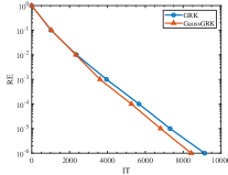
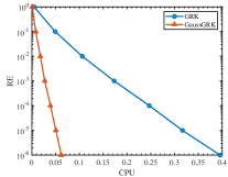
(a) Type I

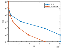
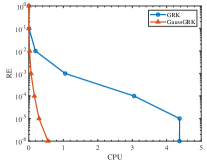
(b) Type II

Fig.  6.1 : The relative errors of GRK and GaussGRK for Types I and II

m	p	$\tau_{1}$	n	q	$\tau_{2}$		GRK	GaussGRK	GRBK	RCD	RK-A	GaussRK-A
50	20	10	20	50	10	IT	8596	8013	112	267	287	291
						CPU	0.3760	0.0609	0.0175	0.0122	0.0089	0.003
100	40	20	40	100	20	IT	38985	37349	94	570	663	643
						CPU	1.8965	0.5035	0.0294	0.0484	0.0335	0.0172
100	40	20	100	500	100	IT	$-$	$-$	26	606	667	648
						CPU	$-$	$-$	0.0573	0.2978	0.1685	0.1465
500	100	50	100	500	50	IT	$-$	$-$	78	1513	1561	1650
						CPU	$-$	$-$	0.1442	4.7249	0.6455	0.9307
1000	200	200	100	500	50	IT	$-$	$-$	24	3122	3242	3322
						CPU	$-$	$-$	0.2241	19.1592	2.5464	4.2424

Table 6.1: The average IT and CPU of GRK, GaussGRK, GRBK, RCD, RK-A, and GaussRK-A with Type I.

From Tables 6.1 and 6.2, we observe that the GRBK method vastly outperforms the RCD, RK-A, and GaussRK-A methods in terms of IT and CPU time, because the GRBK method selects multiple rows and columns in each iteration. Among these methods which select a single row or column for calculation in each iteration, the RK-A and GaussRK-A methods perform slightly better than than the RCD method. In detail, from Table 6.1, we observe that the RCD method requires fewer iteration steps, the GaussRK-A method takes less CPU when the matrix size is small and the RK-A method is more challenging when the matrix size is large. From Table 6.2, we find that the GaussRK-A method is competitive in terms of IT and CPU time.

m	p	n	q		GRK	GaussGRK	GRBK	RCD	RK-A	GaussRK-A
30	10	10	30	IT	50057	11656	1	770	530	256
				CPU	2.0871	0.0708	0.0003	0.0213	0.0139	0.0017
50	20	20	50	IT	$-$	74033	88	2694	1541	825
				CPU	$-$	0.6492	0.0157	0.1233	0.0475	0.0075
100	40	40	100	IT	$-$	$-$	588	7442	4092	2160
				CPU	$-$	$-$	0.0974	0.6245	0.2027	0.0556
100	40	100	500	IT	$-$	$-$	966	5494	3082	1697
				CPU	$-$	$-$	0.2509	2.3004	0.5499	0.2739
500	100	100	500	IT	$-$	$-$	1775	8749	5259	2977
				CPU	$-$	$-$	0.5908	27.2126	2.0268	1.6648
1000	200	100	500	IT	$-$	$-$	3486	18890	10251	5799
				CPU	$-$	$-$	1.4599	116.6466	8.3202	7.4095
1000	200	200	1000	IT	$-$	$-$	7250	$-$	9998	5896
				CPU	$-$	$-$	4.3672	$-$	31.4897	23.0945

Table 6.2: The average IT and CPU of GRK, GaussGRK, GRBK, RCD, RK-A, and GaussRK-A with Type II.

To accelerate the convergence speed, multiple columns (or rows) can be selected in the RCD and RK-A methods instead of a single column (or row) in each iteration, i.e., block versions. We will not experiment and show them here. However, the block variant of the GaussRK-A method is a dense matrix computation, so the computational complexity increases significantly from vector-matrix product to matrix-matrix product.

In Fig.6.2, we plot the relative errors of the GRBK method with different block sizes $\tau_{1}=\tau_{2}=\tau$ for Type I ($A=U_{1}D_{1}V_{1}^{\top}$ with $m=100,p=50,r_{1}=50$ and $B=U_{2}D_{2}V_{2}^{\top}$ with $n=100,q=50,r_{2}=50$). From Fig. 6.2(a), we observe that increasing block sizes leads to a better convergence rate of the GRBK method. From Fig.6.2(b), we can find that as the block sizes $\tau$ increase, the IT and CPU time first decreases, and then increases after reaching the minimum. From Fig.6.2(c), it is easy to see that when $\tau=14,15,16$, the IT and CPU time reach the minimum. The GRK method is the GRBK method with the sizes of block index sets $\left|I_{k}\right|=\left|J_{k}\right|=1$. This also verifies that the GRK method is computationally expensive.

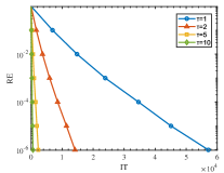
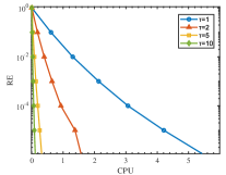
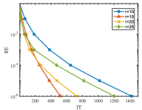
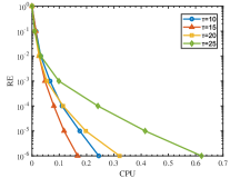
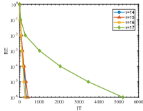
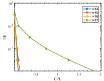
Fig.  6.2 : Relative errors of GRBK with different block sizes $\tau_{1}=\tau_{2}=\tau$ for Type I.

Finally, we also compare them with the RBCD[12] method. To give an intuitive demonstration of the advantage, we define the speed-up as follows:

$$speed-up=\frac{CPU\ of\ RBCD}{CPU\ of\ NEW\ METHOD}.$$

In Fig.6.3, we plot the relative errors of RBCD, RCD, RK-A, GaussRK-A, and GRBK for matrix equation with Type II ($A=randn(100,20)$, $B=randn(20,100)$). For the GRBK method, we use the almost optimal block sizes $\tau_{1}=\tau_{2}=15$. We can see that the RCD, RK-A, GaussRK-A, and GRBK methods are better than the RBCD method in terms of IT and CPU time. From Table 6.3, we see that the IT and CPU of the RCD, RK-A, GaussRK-A, and GRBK methods are smaller than the RBCD methods in terms of both iteration counts and CPU times with significant speed-ups.

	$p\times m$	$50\times 20$	$100\times 20$	$200\times 20$	$500\times 20$	$1000\times 20$
RBCD	IT	4204	1025	376	302	2.0041
	CPU	0.1208	0.0454	0.0342	0.4958	0.0655
RCD	IT	801	353	255	182	169
	CPU	0.0338	0.0226	0.0332	0.3916	1.9815
	speed-up	3.5740	2.0088	1.0301	1.2661	1.0114
RK-A	IT	640	375	280	266	269
	CPU	0.0181	0.0125	0.0181	0.0622	0.7622
	speed-up	6.674	3.6320	1.8895	7.9711	2.6294
GaussRK-A	IT	590	361	284	258	256
	CPU	0.0053	0.0053	0.0117	0.0646	0.9349
	speed-up	22.7925	8.5660	2.9231	7.6749	2.1437
GRBK	IT	70	31	23	19	19
	CPU	0.0135	0.0060	0.0046	0.0041	0.0061
	speed-up	8.9481	7.5667	7.4348	120.9268	328.541

Table 6.3: The average IT, CPU and speed-up of RBCD, RCD, RK-A, GaussRK-A, and GRBK with Type II.

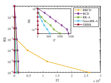
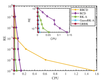
Fig.  6.3 : Relative errors of RBCD, RCD, RK-A, GaussRK-A, and GRBK with Type II.

Example 6.2.

Real-world sparse data. The entries of $A$ and $B$ are selected from the real-world sparse data [18].

Table 6.4 lists the features of these sparse matrices, in which rank(A) denote the rank of the matrix A, respectively, and the density is defined as

$$density=\frac{\text{the number of non-zero elements of an $m$-by-$n$ matrix}}{mn},$$

which indicates the sparsity of the corresponding matrix.

Table 6.4: The detailed features of sparse matrices from [18].

name		size		rank		density
ash219		219 $\times$ 85		85		2.3529%
ash958		958 $\times$ 292		292		0.68493%
divorce		50 $\times$ 9		9		50%
Worldcities		315 $\times$ 100		100		53.625%

Numerical results are shown in Fig.6.4 and Table 6.5. In Fig.6.4, we plot the relative errors of GRBK, RCD, RK-A, and GaussRK-A for the real-world matrix equations. For the GRBK method, we use the block sizes $\tau_{1}=\tau_{2}=15$. In Table 6.5, we report the average IT and CPU of GRK, GaussGRK, GRBK, RCD, RK-A, and GaussRK-A for solving real-world matrix equations. From them, we observe again that the curves of the GRBK methods are decreasing much more quickly than those of the RCD, RK-A, and GaussRK-A methods with respect to the increase of the iteration steps and CPU times. However, as the matrix size increases, the CPU of the GRBK method grows because it takes some time to compute the pseudoinverse. At this time, the RK-A and GaussGRK-A methods are more prominent in terms of IT and CPU times.

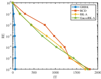
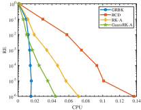
(a) $A=ash219,B=divorce^{\top}$

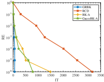
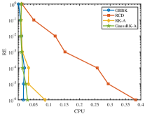
(b) $A=divorce,B=ash219^{\top}$

Fig.  6.4 : Relative errors of GRBK, RCD, RK-A, and GaussRK-A.

A	B	$\tau_{1}$	$\tau_{2}$		GRK	GaussGRK	GRBK	RCD	RK-A	GaussRK-A
ash219	divorce⊤	15	15	IT	$-$	$-$	58	1334	1360	1428
				CPU	$-$	$-$	0.0152	0.1368	0.0713	0.0442
divorce	ash219⊤	15	15	IT	$-$	$-$	67	2559	506	610
				CPU	$-$	$-$	0.0167	0.3823	0.0873	0.0301
divorce	ash219	15	15	IT	$-$	$-$	1632	3024	1204	910
				CPU	$-$	$-$	0.4559	0.3216	0.0684	0.0291
ash958	ash219⊤	15	14	IT	$-$	$-$	5038	6105	5782	5265
				CPU	$-$	$-$	3.2982	20.8641	2.6898	4.2691
ash219	ash958⊤	15	15	IT	$-$	$-$	4976	1792	1709	1718
				CPU	$-$	$-$	3.0925	9.0248	3.7558	3.8908
ash958	Worldcities⊤	15	15	IT	$-$	$-$	34572	5978	5756	5353
				CPU	$-$	$-$	23.6345	26.7466	4.035	6.1356

Table 6.5: The average IT and CPU of GRK, GaussGRK, GRBK, RCD, RK-A and GaussRK-A.

Example 6.3.

CT Data. The test problems of two-dimensional tomography are implemented in the function seismictomo $(N,s,p)$ and the function paralleltomo $(N,\theta,q)$ in the MATLAB package AIR TOOLS [19], where $N$ represents that a cross-section of the subsurface is divided into N equally spaced intervals in both dimensions creating $N^{2}$ cells and $s,p,\theta$ and $q$ denote the number of sources, number of receivers, angle of parallel rays and number of parallel rays. We set $N=40,\ \theta=0:200$ and $q=100$ in the function paralleltomo $(N,\theta,q)$, which generates an exact solution $x_{*}$ of size $1600\times 1$ and $X^{*}=reshape(x_{*},40,40)$, and let $N=30,s=60$ and $p=100$ in the function seismictomo $(N,s,p)$, which generates an exact solution $x_{*}$ of size $900\times 1$ and $X^{*}=reshape(x_{*},30,30)$. For given $p,q$, the entries of $A$ and $B$ are generated from standard normal distributions, i.e., $A=randn(p,m),\ \ B=randn(n,q)$. $C$ is obtained by $C=AX^{*}B$.

All computations start from the initial matrix $X_{0}=O$ and run 4000 iterations on the paralleltomo function and run 5000 iterations on the seismictomo function. In the following experiments, the structural similarity index (SSIM) between the two images X and Y was used to evaluate the quality of the recovered images. SSIM is defined as

$$SSIM=\frac{\left(2\mu_{X}\mu_{Y}+C_{1}\right)\left(2\delta_{XY}+C_{2}\right)}{\left(\mu_{X}^{2}+\mu_{Y}^{2}+C_{1}\right)\left(\delta_{X}^{2}+\delta_{Y}^{2}+C_{2}\right)},$$

where $\mu_{X},\mu_{Y}$ and $\delta_{X}^{2},\delta_{Y}^{2}$ are the means and variances of image $X,Y,$ respectively. $\delta_{XY}$ is the covariance of images X and Y, $C_{1}$ and $C_{2}$ are brightness and contrast constants. The mean of the image represents the brightness of the image and the variance of the image indicates the contrast of the image. Criteria for judging SSIM: SSIM is a number between 0 and 1, and the larger the SSIM value is, the smaller the difference between the two images is. Numerical results are shown in Fig.6.5 and Fig.6.6. The convergence conclusions similar to the previous two groups of experiments are verified again.

(a) Reference image

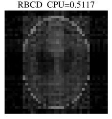
(b) SSIM=0.3658, IT=4000

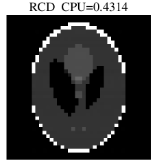
(c) SSIM=0.9992, IT=4000

(d) SSIM=0.9999, IT=4000

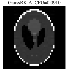
(e) SSIM=1.0000, IT=2764

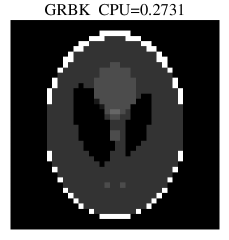
(f) SSIM=1.0000, IT=827

Fig.  6.5 : Performance of the exact figure and five methods for paralleltomo test problem with n = 40.

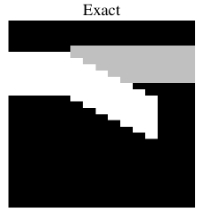
(a) Reference image

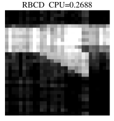
(b) SSIM=0.3782, IT=5000

(c) SSIM=0.9997, IT=2999

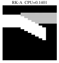
(d) SSIM=0.9998, IT=2620

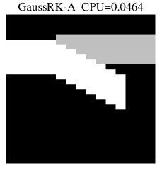
(e) SSIM=0.9999, IT=1549

(f) SSIM=0.9999, IT=158

Fig.  6.6 : Performance of the exact figure and five methods for seismictomo test problem with n = 30.

The maximum number of iterations for all these methods is set no more than 4000. From Fig.6.5 and Fig.6.6, we can see that the RCD, RK-A, GaussRK-A, and GRBK methods recovered by the sketch-and-project method perform better than the RBCD method in terms of both image processing and CPU times. In Fig.6.5, the SSIM value of the recovery image through both the GaussRK-A and GRBK methods is around 1. Since the GRBK method needs to calculate the pseudoinverse, it requires more CPU times than the GaussRK-A method. In Fig.6.6, we can see that all methods have almost recovered this image except the RBCD method.

7 Conclusions

In this paper, we have proposed a sketch-and-project method for solving the matrix equation $AXB=C$. The convergence of the generalized iterative method is explored. Meanwhile, by varying its three parameters, we recover some well-known algorithms as special cases. Numerical experiments show that in a series of methods of vector-matrix product, Gaussian-type methods are competitive in terms of IT and CPU time. It is clear to see that our method allows for a much wider selection of three parameters, which leads to a series of new specific methods. Based on this skecth-and project method, we will investigate new methods for solving nonlinear matrix equations in our future work.

Appendix A Proof for Lemmas

Proof of Lemma 4.3

Proof.

Since $\mathbf{E}\left[A^{2}\right]=\mathbf{E}\left[A^{\top}A\right],\ \mathbf{E}\left[A^{\top}\right]\mathbf{E}\left[A\right]=\left(\mathbf{E}\left[A\right]\right)^{\top}\mathbf{E}\left[A\right]$, to obtain the conclusion, we need to prove $\mathbf{E}\left[A^{\top}A\right]\succeq\mathbf{E}\left[A^{\top}\right]\mathbf{E}\left[A\right],$ i.e.,

$$\mathbf{E}\left[\left(A^{\top}-\mathbf{E}\left[A^{\top}\right]\right)\left(A-\mathbf{E}\left[A\right]\right)\right]\succeq 0.$$

By the definition, it can be seen that for arbitrary column vector $c\in\mathbb{R}^{n}$, $A$ is called a positive semi-definite matrix if $c^{\top}Ac\geq 0$. So we just need to prove that

$$\mathbf{E}\left[c^{\top}\left(A^{\top}-\mathbf{E}\left[A^{\top}\right]\right)\left(A-\mathbf{E}\left[A\right]c\right)\right]\geq 0,$$

i.e.,

$$\mathbf{E}\left[\left(c^{\top}A^{\top}-\mathbf{E}\left[c^{\top}A^{\top}\right]\right)\left(Ac-\mathbf{E}\left[Ac\right]\right)\right]\geq 0.$$

Since $A\in\mathbb{R}^{n\times n}$, $Ac\in\mathbb{R}^{n}$ is a column vector. For convenience, let $c^{\top}A^{\top}=(y_{1},y_{2},...,y_{n})=Y^{\top}$, we have

$$\begin{split}\mathbf{E}\left[\left(Y^{\top}-\mathbf{E}\left[Y^{\top}\right]\right)\left(Y-\mathbf{E}\left[Y\right]\right)\right]&=\mathbf{E}\left[Y^{\top}Y-\mathbf{E}\left[Y^{\top}\right]Y-Y^{\top}\mathbf{E}\left[Y\right]+\mathbf{E}\left[Y^{\top}\right]\mathbf{E}\left[Y\right]\right]\\ &=\mathbf{E}\left[Y^{\top}Y\right]-\mathbf{E}\left[Y^{\top}\right]\mathbf{E}\left[Y\right]-\mathbf{E}\left[Y^{\top}\right]\mathbf{E}\left[Y\right]+\mathbf{E}\left[Y^{\top}\right]\mathbf{E}\left[Y\right]\\ &=\mathbf{E}\left[Y^{\top}Y\right]-\mathbf{E}\left[Y^{\top}\right]\mathbf{E}\left[Y\right]\\ &=\mathbf{E}\left[y_{1}^{2}+y_{2}^{2}+...+y_{n}^{2}\right]-\left[\left(\mathbf{E}\left[y_{1}\right]\right)^{2}+\left(\mathbf{E}\left[y_{2}\right]\right)^{2}+...+\left(\mathbf{E}\left[y_{n}\right]\right)^{2}\right]\\ &=Dy_{1}+Dy_{2}+...+Dy_{n}\geq 0,\end{split}$$

where $Dy_{i}$ is the variance $y_{i}$ for $i=1,2,\cdots,n$. Therefore, $\mathbf{E}\left[\left(A^{\top}-\mathbf{E}\left[A^{\top}\right]\right)\left(A-\mathbf{E}\left[A\right]\right)\right]$ is positive semi-definite. ∎

Proof of Lemma 4.7

Proof.

For $\forall X_{2}\in M_{2}$, then $\exists Y_{2}\ s.t.\ A^{\top}AY_{2}BB^{\top}=X_{2}$. Let $Y_{1}=AY_{2}B$, there exsits

$$A^{\top}AY_{2}BB^{\top}=A^{\top}Y_{1}B^{\top}=X_{2},$$

which means $X_{2}\in M_{1}$.

For $\forall X_{1}\in M_{1}$, then $\exists Y_{1}\ s.t.\ A^{\top}Y_{1}B^{\top}=X_{1}$, which means matrix equation $A^{\top}XB^{\top}=C$ has a solution. Hence, we konw that $A^{\top}(A^{\top})^{{\dagger}}X_{1}(B^{\top})^{{\dagger}}B^{\top}=X_{1}$. Based on the nature of the pseudoinverse, we can obtain

$$(A^{\top})^{{\dagger}}=(A^{{\dagger}})^{\top}=(A^{{\dagger}}AA^{{\dagger}})^{\top}=\left(A^{{\dagger}}(AA^{{\dagger}})\right)^{\top}=(AA^{{\dagger}})^{\top}(A^{{\dagger}})^{\top}=AA^{{\dagger}}(A^{{\dagger}})^{\top},$$

$$(B^{\top})^{{\dagger}}=(B^{{\dagger}})^{\top}=(B^{{\dagger}}BB^{{\dagger}})^{\top}=\left((B^{{\dagger}}B)B^{{\dagger}}\right)^{\top}=(B^{{\dagger}})^{\top}(B^{{\dagger}}B)^{\top}=(B^{{\dagger}})^{\top}B^{{\dagger}}B.$$

Thus $X_{1}$ can be written as $X_{1}=A^{\top}AA^{{\dagger}}(A^{{\dagger}})^{\top}X_{1}(B^{{\dagger}})^{\top}B^{{\dagger}}BB^{\top}=A^{\top}AW_{2}BB^{\top}$ where $W_{2}=A^{{\dagger}}(A^{{\dagger}})^{\top}X_{1}(B^{{\dagger}})^{\top}B^{{\dagger}}$. It holds

$$A^{\top}Y_{1}B^{\top}=A^{\top}AW_{2}BB^{\top}=X_{1}.$$

Thus, $X_{1}$ is also in the set $M_{2}$. Therefore, $M_{1}=M_{2}.$ ∎

Proof of Lemma 3.1

Proof.

For any matrix $M$, the pseudoinverse satisfies the identity $M^{\dagger}MM^{\dagger}=M^{\dagger}$. Let $M=S^{\top}AG^{-1}A^{\top}S$, we get

$$\begin{split}\left(Z_{1}^{\prime}\right)^{2}&=G^{-1}A^{\top}S\left(S^{\top}AG^{-1}A^{\top}S\right)^{\dagger}S^{\top}AG^{-1}A^{\top}S\left(S^{\top}AG^{-1}A^{\top}S\right)^{\dagger}S^{\top}A\\ &=G^{-1}A^{\top}SM^{\dagger}MM^{\dagger}S^{\top}A\\ &=G^{-1}A^{\top}SM^{\dagger}S^{\top}A\\ &=G^{-1}A^{\top}S\left(S^{\top}AG^{-1}A^{\top}S\right)^{\dagger}S^{\top}A=Z_{1}^{\prime},\end{split}$$

then have

$$\left(Z_{2}\otimes Z_{1}^{\prime}\right)^{2}=\left(Z_{2}\otimes Z_{1}^{\prime}\right)\left(Z_{2}\otimes Z_{1}^{\prime}\right)=Z_{2}^{2}\otimes\left(Z_{1}^{\prime}\right)^{2}=Z_{2}\otimes Z_{1}^{\prime},$$

and thus both $Z_{2}\otimes Z_{1}^{\prime}$ and $I-Z_{2}\otimes Z_{1}^{\prime}$ are projection matrices. To show that $Z_{2}\otimes Z_{1}^{\prime}$ is an orthogonal projection with respect to the $\left(I\otimes G\right)$-inner product, we need to verify that $\left(Z_{2}\otimes Z_{1}^{\prime}\right)\left[(BP)\otimes\left(G^{-1}A^{\top}S\right)\right]=(BP)\otimes(G^{-1}A^{\top}S)$ and for every $y\in Null\left((P^{\top}B^{\top})\otimes(S^{\top}A)\right)$ there exists $\left(Z_{2}\otimes Z_{1}^{\prime}\right)y=0$.

The first relation is obtained from the properties of the pseudoinverse: $\left(M^{\top}M\right)^{\dagger}M^{\top}=M^{\dagger}$ and $MM^{\dagger}M=M$. Setting $M=G^{-\frac{1}{2}}A^{\top}S$, we have

$$\begin{split}Z_{1}^{\prime}\left(G^{-1}A^{\top}S\right)&=G^{-1}A^{\top}S\left(S^{\top}AG^{-1}A^{\top}S\right)^{\dagger}S^{\top}AG^{-1}A^{\top}S\\ &=G^{-\frac{1}{2}}M\left(M^{\top}M\right)^{\dagger}M^{\top}M\\ &=G^{-\frac{1}{2}}MM^{\dagger}M\\ &=G^{-\frac{1}{2}}M\\ &=G^{-\frac{1}{2}}G^{-\frac{1}{2}}A^{\top}S=G^{-1}A^{\top}S.\end{split}$$

Similarly, denoting $M=BP$, we have

$$\begin{split}Z_{2}BP&=BP\left(P^{\top}B^{\top}BP\right)^{\dagger}P^{\top}B^{\top}BP\\ &=M\left(MM^{\dagger}\right)M^{\top}M\\ &=MM^{\dagger}M=M=BP.\end{split}$$

Thus the first relation holds. For the second relation, it exists

$$\begin{split}\left(Z_{2}\otimes Z_{1}^{\prime}\right)y=&\left\{\left[BP\left(P^{\top}B^{\top}BP\right)^{\dagger}P^{\top}B^{\top}\right]\otimes\left[G^{-1}A^{\top}S\left(S^{\top}AG^{-1}A^{\top}S\right)^{\dagger}S^{\top}A\right]\right\}y\\ =&\left\{\left[BP\left(P^{\top}B^{\top}BP\right)^{\dagger}\right]\otimes\left[G^{-1}A^{\top}S\left(S^{\top}AG^{-1}A^{\top}S\right)^{\dagger}\right]\right\}\\ &\left[(P^{\top}B^{\top})\otimes(S^{\top}A)\right]y\\ =&0.\end{split}$$

∎

Proof of Lemma 4.1

Proof.

Let $\widetilde{Z_{1}}=GZ_{1}^{\prime}$. Since $\mathbf{E}\left[Z_{2}\otimes\widetilde{Z_{1}}\right]$ is invertible and $G^{-\frac{1}{2}}\widetilde{Z_{1}}G^{-\frac{1}{2}}$ is an idempotent matrix, the spectrum of $\left(I\otimes G^{-\frac{1}{2}}\right)\left(Z_{2}\otimes\widetilde{Z_{1}}\right)\left(I\otimes G^{-\frac{1}{2}}\right)$ is contained in $\left\{0,1\right\}$, we have$\left(I\otimes G^{-\frac{1}{2}}\right)\mathbf{E}\left[Z_{2}\otimes\widetilde{Z_{1}}\right]\left(I\otimes G^{-\frac{1}{2}}\right)$ is positive definite. With

$$\begin{split}\rho&=1-\lambda_{min}\left(\mathbf{E}\left[Z_{2}\otimes Z_{1}^{\prime}\right]\right)\\ &=1-\lambda_{min}\left(\mathbf{E}\left[Z_{2}\otimes\left(G^{-\frac{1}{2}}\widetilde{Z_{1}}G^{-\frac{1}{2}}\right)\right]\right).\end{split}$$

it holds $\rho<1$. If $B^{\top}\otimes A$ is not full column rank, then there would be $0\neq x\in\mathbb{R}^{nm}$ such that $\left(B^{\top}\otimes A\right)x=0$. Therefore, we have $\widetilde{Z_{1}}XZ_{2}=0$ and $\mathbf{E}\left[Z_{2}^{T}\otimes\widetilde{Z_{1}}\right]vec(X)=0$, which contradicts the assumption that $\mathbf{E}\left[Z_{2}^{T}\otimes\widetilde{Z_{1}}\right]$ is invertible. Analogously, $(BP)^{\top}\otimes(S^{T}A)$ is also full column rank. Finally, since $B^{\top}\otimes A$ is full column rank, $X^{*}$ must be unique (recall that assume throughout the paper that $AXB=C$ is consistent). ∎

Proof of Lemma 5.3

Proof.

Using the properties of Kronecker product and considering the matrices are symmetric semi-definite, we have

$$\lambda_{\min}\left(A^{\top}\otimes B\right)=\lambda_{\min}\left(A\right)\lambda_{\min}\left(B\right).$$

To prove (5.11), we only need to demonstrate that

$$\lambda_{\min}\left(A_{2}\right)\lambda_{\min}\left(B_{2}\right)\geq\lambda_{\min}\left(A_{1}\right)\lambda_{\min}\left(B_{1}\right).$$

Since $A_{2}$ and $A_{2}-A_{1}$ are symmetric positive definite matrices, by Lemma 5.2 we can obtain the following inequality

$$0\leq\lambda_{\min}\left(A_{2}-A_{1}\right)\leq\lambda_{\min}\left(A_{2}\right)+\lambda_{\max}\left(-A_{1}\right).$$

From the fact that $\lambda_{\max}\left(-A_{1}\right)=-\lambda_{\min}\left(A_{1}\right)$, hence it results in

$$0\leq\lambda_{\min}\left(A_{2}-A_{1}\right)\leq\lambda_{\min}\left(A_{2}\right)-\lambda_{\min}\left(A_{1}\right).$$

Therefore, we get

$$\lambda_{\min}\left(A_{2}\right)\geq\lambda_{\min}\left(A_{1}\right)\geq 0.$$ (A.1)

Similarly, for $B_{1},B_{2}$, there exists

$$\lambda_{\min}\left(B_{2}\right)\geq\lambda_{\min}\left(B_{1}\right)\geq 0.$$ (A.2)

Combining (A.1) and (A.2), we can obtain $\lambda_{\min}\left(A_{2}\right)\lambda_{\min}\left(B_{2}\right)\geq\lambda_{\min}\left(A_{1}\right)\lambda_{\min}\left(B_{1}\right)$, i.e., $\lambda_{\min}\left(A_{2}^{\top}\otimes B_{2}\right)\geq\lambda_{\min}\left(A_{1}^{\top}\otimes B_{1}\right).$ The proof is completed. ∎

References

• Lin et al. [2018] H. Lin, T. Maekawa, C. Deng, Survey on geometric iterative methods and their applications, Computer Aided Design 95 (2018) 40–51.
• Regalia and Mitra [1989] P. A. Regalia, S. K. Mitra, Kronecker products, unitary matrices and signal processing applications, SIAM Review 31 (1989) 586–613.
• Hua [1990] D. Hua, On the symmetric solutions of linear matrix equations, Linear Algebra and its Applications 131 (1990) 1–7.
• Zha [1995] H. Zha, Comments on Large Least Squares Problems Involving Kronecker Products, volume 16, Society for Industrial and Applied Mathematics, USA, 1995.
• Ding and Chen [2005] F. Ding, T. Chen, Iterative least-squares solutions of coupled Sylvester matrix equations, Systems and Control Letters 54 (2005) 95–107.
• Wang et al. [2013] X. Wang, Y. Li, L. Dai, On Hermitian and skew-Hermitian splitting iteration methods for the linear matrix equation AXB=C, Computers and Mathematics with Applications 65 (2013) 657–664.
• Tian et al. [2017] Z. Tian, M. Tian, Z. Liu, T. Xu, The Jacobi and Gauss–Seidel–type iteration methods for the matrix equation AXB=C, Applied Mathematics and Computation 292 (2017) 63–75.
• Cvetković-Ilić [2008] D. S. Cvetković-Ilić, Re-nnd solutions of the matrix equation AXB=C, Journal of the Australian Mathematical Society 84 (2008).
• Peng [2010] Z. Peng, A matrix LSQR iterative method to solve matrix equation AXB=C, International Journal of Computer Mathematics 87 (2010) 1820–1830.
• Niu and Zheng [2022] Y. Niu, B. Zheng, On global randomized block Kaczmarz algorithm for solving large-scale matrix equations, arXiv MATH Numerical Analysis (2022) arXiv:2204.13920.
• Wu et al. [2022] N. Wu, C. Liu, Q. Zuo, On the Kaczmarz methods based on relaxed greedy selection for solving matrix equation AXB=C, Journal of Computational and Applied Mathematics 413 (2022).
• Du et al. [2022] K. Du, C. Ruan, X. Sun, On the convergence of a randomized block coordinate descent algorithm for a matrix least squares problem, Applied Mathematics Letters 124 (2022) 1660–1690.
• Shafiei and Hajarian [2022] S. G. Shafiei, M. Hajarian, Developing Kaczmarz method for solving Sylvester matrix equations, Journal of the Franklin Institute 359 (2022) 8991–9005.
• Gower and Richtárik [2015] R. M. Gower, P. Richtárik, Randomized iterative methods for linear systems, SIAM Journal on Matrix Analysis and Applications 36 (2015) 1660–1690.
• Simoncini [2016] V. Simoncini, Computational methods for linear matrix equations, SIAM Review 58 (2016) 377–441.
• Graham [1981] A. Graham, Kronecker Products and Matrix Calculus: with Applications, Ellis Horwood Ltd, 1981.
• Golub and Van Loan [2013] G. H. Golub, C. F. Van Loan, Matrix Computations, The Johns Hopkins University Press, Baltimore, 4th edition, 2013.
• Davis and Hu [2011] T. A. Davis, Y. Hu, The University of Florida Sparse Matrix Collection, ACM Transactions on Mathematical Software 38 (2011).
• Hansen and Jórgensen [2018] P. C. Hansen, J. S. Jórgensen, AIR Tools II: algebraic iterative reconstruction methods, improved implementation, Numerical Algorithms 79 (2018) 107–137.