Control and Readout of a 13-level Trapped Ion Qudit

Abstract

To implement useful quantum algorithms which demonstrate quantum advantage, we must scale currently demonstrated quantum computers up significantly. Leading platforms such as trapped ions face physical challenges in including more information carriers. A less explored avenue for scaling up the computational space involves utilizing the rich energy level structure of a trapped ion to encode multi-level qudits rather than two-level qubits. Here we show control and single-shot readout of qudits with up to 13 computational states, using protocols which can be extended directly to manipulate qudits of up to 25 levels in our chosen information host, ^137Ba^+. This represents more than twice as many computational states per qudit compared with prior work in trapped ions[1]. In addition to the preparation and readout protocols we demonstrate, universal quantum computation requires other quantum logic primitives such as entangling gates. These primitives have been demonstrated for lower qudit dimensions and can be directly generalized to the higher dimensions we employ. Hence, our advance opens an avenue towards using high-dimensional qudits for large-scale quantum computation. We anticipate efficiently utilizing available energy states in a trapped ion to play a significant and complementary role in tackling the challenge in scaling up the computational space of a trapped ion quantum computer. A qudit architecture also offers other practical benefits, which include affording relaxed fault tolerance thresholds for quantum error correction [2, 3, 4, 5, 6], providing an avenue for efficient quantum simulation of higher spin systems [7, 8], and more efficient qubit gates [9, 10].

Main

Realizing quantum computation involves encoding quantum information in a physical system, such as atomic energy states, quantized states of superconducting circuits, and polarization states of photons [11]. Trapped ions are a promising platform because of the high fidelities of the quantum operations [12], where gate errors below the quantum error correcting code threshold have been empirically achieved [13]. Another attractive feature of trapped ions is the certainty that all ions are identical to each other by nature. This mitigates the increasing complexities of hardware calibrations required when scaling up a system with non-homogeneous quantum information carriers [14].

Conventional quantum computing approaches encode two computational states in a quantum information unit, called a qubit. However, most platforms naturally exhibit more than two quantum states per information carrier, and it is not obvious why only two states should be utilized. By encoding a general number of computational states, $d$, one defines a qudit. Scaling up to a higher value of $d$ provides a direct increase of the computational Hilbert space given a constraint on the number of information carriers. This constraint is relevant to trapped ions, as there are technical limitations to the number of ions which can be coherently controlled in a single ion chain [12]. High-dimensional qudit encodings can therefore complement other trapped ion scaling efforts, such as the use of ion trap arrays [15] or photonic interconnects [16], to further increase the computational Hilbert space. There are other advantages of a qudit quantum system, which include a more relaxed quantum error correction threshold [2, 3, 4, 5, 6], more direct higher spin quantum simulations [7, 8], and more efficient qubit gates [9, 10].

Higher-dimensional atomic qudits have received increasing attention in recent years [17, 7, 18, 19, 20], including a demonstration of universal quantum computing with 5-level trapped ion qudits [1]. In this work, we demonstrate state preparation and measurement (SPAM) of a 13-level qudit, which more than doubles the number of qudit levels implemented in a single trapped ion [1]. This advance is made possible by exploiting the abundant stable and metastable energy levels in ^137Ba^+, which enables qudit encodings of up to 25 levels with the protocol presented in this work. The richer energy level structure of ^137Ba^+ comes with non-trivial complexities in understanding the transition frequencies and strengths, which we resolve by constructing predictive theoretical models that match empirical data. This understanding is crucial for any researchers aspiring to use ^137Ba^+ or other ion species with similar energy level structures for high-dimensional qudit work. We demonstrate an average 13-level SPAM fidelity of $91.7\pm 0.3\%$, and the major sources of errors are technical with known solutions. The calibration times for the SPAM parameters do not increase with $d$ for $d\geq 6$ with the protocols that we present in this work. Our results demonstrate the feasibility of efficiently utilizing high numbers of trapped ion energy levels, and are a stepping stone towards high-dimensional qudit quantum computing.

Energy Levels and Qudit Encoding

#

(a)

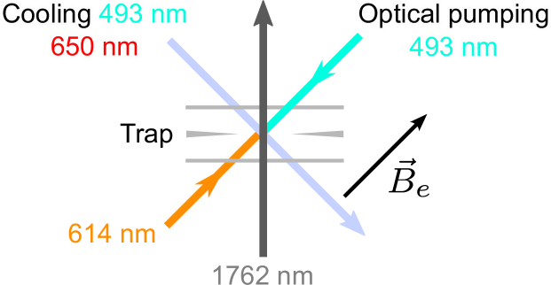
(b)

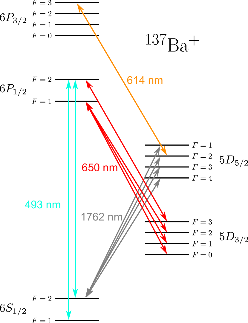
(c)

Figure 1: (a) Qudit encoding schemes for ^137Ba^+. Black texts indicate the encoding scheme employed in this work for ^137Ba^+. All states with sufficiently strong (resulting in $\pi$-pulse transition fidelity of $\geq 75\%$, discussed later in main text) allowed transitions to the $5D_{5/2}$ level from $\lvert 0\rangle$ are encoded. Gray texts indicate a possible extension of the encoding scheme to up to 25 levels, where the additional states are chosen arbitrarily. (b) Illustration of the optical setup in this work. $\vec{B}_{e}$ denotes the magnetic field. See Extended Fig. E1 for detailed illustration of the setup. (c) The ^137Ba^+ energy level structure of the energy levels relevant to this work. $\qty{493}{\nano}$ and $\qty{650}{\nano}$ lasers are used for laser cooling and fluorescent readout of the ion. Metastable states in the $5D_{5/2}$ level are accessed from the $6S_{1/2}$ ground level with a 1762 laser. A 614 laser is used to reset the experiments by pumping states out of the $5D_{5/2}$ level to the $6P_{3/2}$ level, which undergoes fast decay mostly to the ground level.

In a static non-zero magnetic field, ^137Ba^+ has 8 distinct stable energy states in the $6S_{1/2}$ level and 24 distinct metastable energy states (with a lifetime of $\qty{35}{}$ [21]) in the $5D_{5/2}$ level (see Fig. 1(a)). The lifetime of the $5D_{5/2}$ metastable states is orders of magnitude larger than a typical quantum operation time scale [13, 1], so this abundance of stable or metastable states in ^137Ba^+ makes it an excellent candidate for high-dimensional qudit encoding.

The measurement procedures used in this article allow 25 of the 32 states in the $6S_{1/2}$ and $5D_{5/2}$ levels to be distinguishable in a single shot (discussed in next sections), thus allowing qudit encodings of up to 25 levels in principle. In this work, we encode computational states in the $\lvert 6S_{1/2},F=2,m_{F}=2\rangle$ state and the subset of $5D_{5/2}$ states accessible from the $\lvert 6S_{1/2},F=2,m_{F}=2\rangle$ state using quadrupole-allowed 1762 transitions. We exclude $5D_{5/2}$ states with $\pi$-pulse transition fidelities of $\leq 75\%$ (see Supplementary Information), resulting in a 13-level encoding, illustrated in Fig. 1(a).

Fig. 1(b) illustrates the setup used in this work for optical control of the ^137Ba^+ energy levels (see Methods and Extended Fig. E1 for more details). To attain sufficient experimental controls to perform SPAM, other energy levels in ^137Ba^+ are utilized. The relevant energy levels and their corresponding laser frequencies for control are summarized in Fig. 1(c).

Note that we have labelled the states using $\tilde{F}$ and $m_{\tilde{F}}$ notations in Fig. 1(a), which we define as the energy eigenstates of the ion in a general magnetic field strength, $B_{e}$. Each $\lvert\tilde{F},m_{\tilde{F}}\rangle$ state approaches the corresponding $\lvert F,m_{F}\rangle$ state at low magnetic field strengths, i.e. $\lvert\tilde{F},m_{\tilde{F}}\rangle\approx\lvert F,m_{F}\rangle$ as $B_{e}\rightarrow 0$. This distinction is necessary as the hyperfine energy level splitting between the $F=3$ and $F=4$ states in the $5D_{5/2}$ level is small, at $\qty{486}{\kilo}$ [22], and the linear Zeeman approximation does not hold for typical values of $B_{e}$, as indicated by the strong overlap between $F=3$ and $F=4$ energies in Fig. 2(a). Fig. 2(b) illustrates this effect further; it can be seen that $\lvert 5D_{5/2},\tilde{F}=4,m_{\tilde{F}=1}\rangle$ state differs significantly from $\ket{F=4,m_{F}=1}$ for external fields as low as 0.2G. This trend applies to other states with $\tilde{F}=3$ and $\tilde{F}=4$, except for states with $m_{\tilde{F}}=\pm 4$ (see Extended Figs. E2, E3, E4). To suppress coherent dark states [23], which is a prerequisite for ion cooling and fluorescence readout, it is necessary to apply an external field of more than 0.2G, and therefore necessary to work in the regime where the energy eigenstates of the $5D_{5/2}$ level differ significantly from the $\lvert F,m_{F}\rangle$ states. In this work, the magnetic field strength is estimated to be $B_{e}=\qty{8.35}{G}$ (see Fig. 2(a)), well within the regime where the linear Zeeman approximation breaks down.

The discrepancies between the $5D_{5/2}$ energy eigenstates and the $\lvert F,m_{F}\rangle$ states result in $6S_{1/2}\leftrightarrow 5D_{5/2}$ transition strengths that differ significantly from those calculated in the $\lvert F,m_{F}\rangle$ basis. From Fig. 2(c), the numerically simulated (see Methods) and empirically measured relative transition strengths at 8.35G are much weaker for $\tilde{F}=3$ states as compared to $\tilde{F}=4$ states, starting from the $\ket{6S_{1/2},\tilde{F}=2,\tilde{m}=2}$ state. This deviates significantly from what is predicted assuming $\lvert F,m_{F}\rangle$ states (not shown). Despite these changes in transition strengths, we nevertheless calculate that all states in the $5D_{5/2}$ level are practically accessible (with transition strengths within an order of magnitude of the strongest transitions, see Extended Data Table E1).

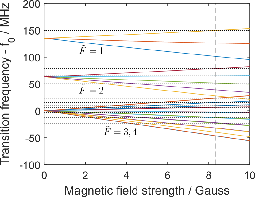
(a)

(b)

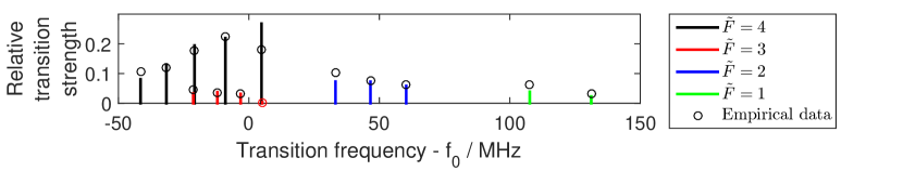
(c)

Figure 2: (a) Simulated transition energy levels to the $5D_{5/2}$ states from the $\lvert\tilde{F}=2,m_{\tilde{F}}=2\rangle$ state in the $6S_{1/2}$ level. $f_{0}$ is the transition frequency to the $F=4$ level at zero magnetic field strength. The horizontal dotted lines indicate the empirically measured transition frequencies, which match well with the simulated transition frequency splittings at 8.35G, marked by the vertical dashed line. (b) A representative plot of the simulated energy eigenstates, illustrating the mixing of the zero-field eigenstates. The $\lvert\tilde{F}=4,m_{\tilde{F}}=1\rangle$ energy eigenstate is expressed in the $\lvert F,m_{F}\rangle$ basis for magnetic field strengths from 0 to 10G. Components with zero amplitudes are not plotted. (c) (Color online) Theoretically estimated non-zero transition strengths to the $5D_{5/2}$ states from the $\lvert 6S_{1/2},\tilde{F}=2,m_{\tilde{F}}=2\rangle$ state, relative to the reduced transition matrix element (see Methods). The empirical data are scaled values of the measured Rabi frequencies. The error bars of the empirical data are smaller than the plot markers and are not plotted. The $\lvert\tilde{F}=3,m_{\tilde{F}}=3\rangle$ relative transition strength is too weak to be clearly visible on the plot or accurately estimated experimentally due to coherence time limitations. The red marker is an upper bound of the empirically measured Rabi frequency for this transition.

State Preparation

In this work, we initialize the ^137Ba^+ in the $\lvert 6S_{1/2},F=2,m_{F}=2\rangle$ state, which we encode as the $\lvert 0\rangle$ state. This is done via optical pumping by sending $\sigma^{+}$-polarized 493 light to the ion, together with 650 light (see Fig. 1(b)), with laser frequencies as shown in Fig. 1(c). In this work, to prepare the ion in any of the $\lvert n\neq 0\rangle$ states, a $\pi$-pulse of $\qty{1762}{\nano}$ light with the corresponding frequency to drive the $\lvert 0\rangle\leftrightarrow\lvert n\rangle$ transition is applied to the ion. In general, to encode up to 25 levels, any desired state can be prepared with at most three sequential 1762 laser transitions.

State Measurement

^137Ba^+ emits fluorescence when it is driven by $\qty{493}{\nano}$ and $\qty{650}{\nano}$ lasers if the ion is in the $6S_{1/2}$ state. It does not fluoresce if the ion is in any of the encoded $5D_{5/2}$ states. We make use of this property to construct a single-shot qudit measurement process, which is described in the sequence below and sketched in Fig. 3(a). The process consists of multiple steps, but we characterize it as single-shot in the sense that the projected quantum state can be determined definitively in a single run of the measurement protocol.

1. Without loss of generality, the $\lvert 0\rangle$ state is assigned as one of the $6S_{1/2}$ states. Any population of the encoded states in the $6S_{1/2}$ level other than state $\lvert 0\rangle$ is brought up to a corresponding unencoded $5D_{5/2}$ state by sending $\pi$-pulses of 1762 laser with frequencies resonant to the desired transitions in sequence. We call this a shelving process.

2. The 493 and 650 lasers are turned on to check for fluorescence. The ion is measured to be in the qudit state $\lvert 0\rangle$ if fluorescence is observed at this step.

3. The population corresponding to the next computational state $\lvert n\rangle$ in $5D_{5/2}$ is brought down to one of the $6S_{1/2}$ states by sending a $\pi$-pulse of $\qty{1762}{\nano}$ laser with the corresponding transition frequency. We call this a de-shelving process.

4. Step 2 is repeated to check for fluorescence. The ion is measured to be in the qudit state $\lvert n\rangle$ if fluorescence is observed for the first time at this step, as exemplified in Fig. 3(b).

5. Steps 3 and 4 are repeated until all states are de-shelved and checked for fluorescence.

For the qudit encoding demonstrated in this article, as shown in Fig. 1(a), the shelving process in Step 1 is unnecessary. The $6S_{1/2}$ ground state chosen for the de-shelving process is also fixed to be $\lvert 6S_{1/2},F=2,m_{F}=2\rangle$ for convenience. Fig. 3(a) summarizes the simplified pulse sequence for performing SPAM as described here. From this measurement protocol, it can be seen from Step 1 that 7 out of the 32 stable/metastable states need to be left unencoded to achieve full distinguishability, resulting in a maximum encoding of 25 states.

SPAM Experimental Results and Discussion

#

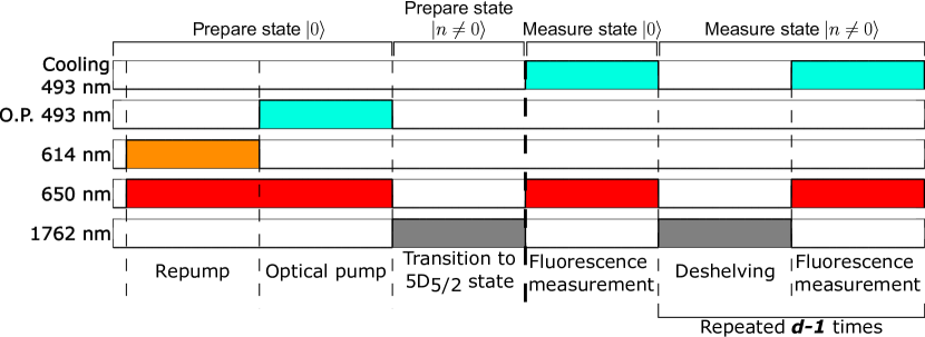
(a)

(b)

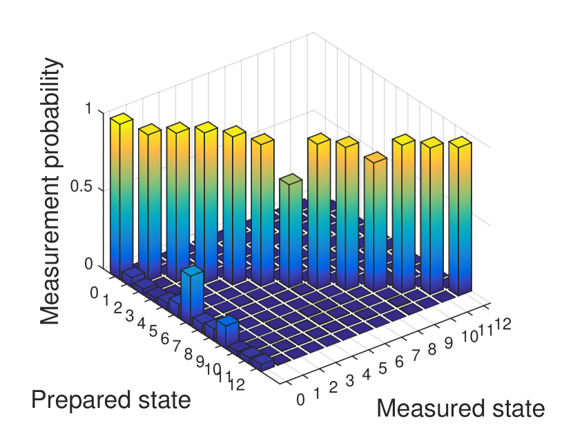
(c)

Figure 3: (a) Simplified pulse sequence for one SPAM experiment for a prepared state $\lvert n\rangle$ of a $d$-dimensional qudit, demonstrated in this work for $d=13$. O.P. denotes optical pumping. The time axis is not drawn to scale. The pulse sequences to the left and right of the bold dashed line are the state preparation and state measurement processes respectively. The 1762 laser pulse for the state preparation step is only needed if the prepared state is not $\lvert 0\rangle$. For a detailed pulse sequence relevant to the experimental apparatus, see extended Fig. E5. (b) Examples of measurement outcomes. B and D denote that the ion is detected as bright and dark respectively. The de-shelving process in the measurement sequence as described in the main text is performed in ascending order of the encoded states. Experiments 1 and 2 are interpreted as measuring the system to be in state $\lvert 3\rangle$. Experiment 3 is regarded as a measurement failure and is removed from the data set for the post-selected SPAM results. In this experiment, the deshelving process is simultaneously a reshelving process (see Extended Fig. E5). An alternative interpretation that treats Experiment 2 as a measurement failure rather than a measurement of the state $\ket{3}$ is discussed in the Supplementary Information. (c) Post-selected measurement probability of the 13-level qudit SPAM experiment.

Fig. 3(b) shows representative examples of possible measurement outcomes. Experiment 3 in Fig. 3(b) is a directly detectable failure of the measurement procedure. This is arguably a less critical error than misdiagnosing the quantum state, as the user directly knows an error has occurred and can rerun the computation. Fig. 3(c) summarizes the post-selected SPAM experimental results, where the cases when no bright state is detected throughout the measurement sequence are removed from the data set. For the raw SPAM results, where the cases with no bright states detected are counted as errors, see Extended Data Table E3. The average raw and post-selected SPAM errors are computed to be $13.1\pm 0.3\%$ and $8.3\pm 0.3\%$ respectively for a 13-level qudit. The raw data sets and analysis scripts for this work can be found in the repository linked at Ref. [24].

We conclude that the magnetic field noise is a major source of error in this work, using the following error analysis. The post-selected SPAM error for a given prepared state $\ket{n\neq 0}$ due to decoherence from magnetic field noise is

$$\epsilon_{SPAM}=\frac{\epsilon_{\pi}}{\epsilon_{\pi}+\left(1-\epsilon_{\pi}\right)^{2}},$$ (1)

where $\epsilon_{\pi}$ is the error for a single $\pi$-pulse transition. Using filter function theory [25, 26], $\epsilon_{\pi}$ can be expressed as

$$\epsilon_{\pi}=\frac{1}{2}\left(1-e^{-\chi}\right),$$ (2)

where $\chi$ is a spectral overlap of the transition frequency noise power spectral density (PSD), $S\left(\omega\right)$, with the filter function of the target operation, $F\left(\omega\right)$

$$\chi=\frac{1}{\pi}\int_{0}^{\infty}\frac{1}{\omega^{2}}S\left(\omega\right)F\left(\omega\right)d\omega.$$ (3)

Assuming the magnetic field noise to be a $1/f$ noise with a spectral peak at the mains electricity frequency and a baseline white noise, $\chi$ can be derived to scale as

$$\chi\propto\kappa^{2}\tau_{\pi}^{2},$$ (4)

where $\kappa$ is the magnetic field sensitivity of the transition frequency and $\tau_{\pi}$ is the $\pi$-pulse time. See Supplementary Information for the derivation of Eq. 4. The scaling of $\epsilon_{SPAM}$ with $\kappa^{2}\tau_{\pi}^{2}$ as shown in Fig. 4(a) shows agreement with this error model, which supports the notion that magnetic field noise is a major source of error in this work. This simplified model may also be useful for predicting which of the 126 allowed quadrupole transitions between $6S_{1/2}$ and $5D_{5/2}$ states will be most useful for quantum operations as the 1762 nm laser orientation and polarization are varied.

The vertical intercept of $\epsilon_{SPAM}=0.04\pm 0.01$ in Fig. 4(a) may indicate that around 4% of the error comes from other sources. Around $1.5\pm 2\%$ of the remaining error is estimated to be from drifts of the experimental parameters from the time of calibration to the time SPAM experiments are done (see Supplementary Information). We speculate that the majority of the rest of the remaining error to be from unclean laser polarization from the optical pumping step, but the available data in this work does not allow accurate quantitative estimations of the remaining errors. A more complex state preparation protocol [27] has been shown to reduce optical pumping errors to below $10^{-4}$, and can be applied in the future extension of this work with sufficient hardware upgrades. We estimated errors from other known error sources (from spontaneous decay from the $5D_{5/2}$ level, off-resonant transition error and bright/dark state discrimination error) and found that they contribute less than $0.5\%$ of error (see Supplementary Information).

Because the magnetic field noise is a dominant source of error, the fidelity is highly dependent on the choice of qudit states. We study the best- and worst-case SPAM fidelities for qudits of differing dimension in Fig. 4(b), always including the state $\ket{0}$. The fact that it is possible to choose qudit encodings where the errors improve with higher dimension indicate that our results are not limited by any effects that intrinsically depend on the qudit dimension.

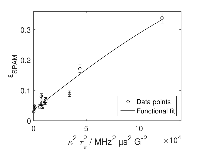
(a)

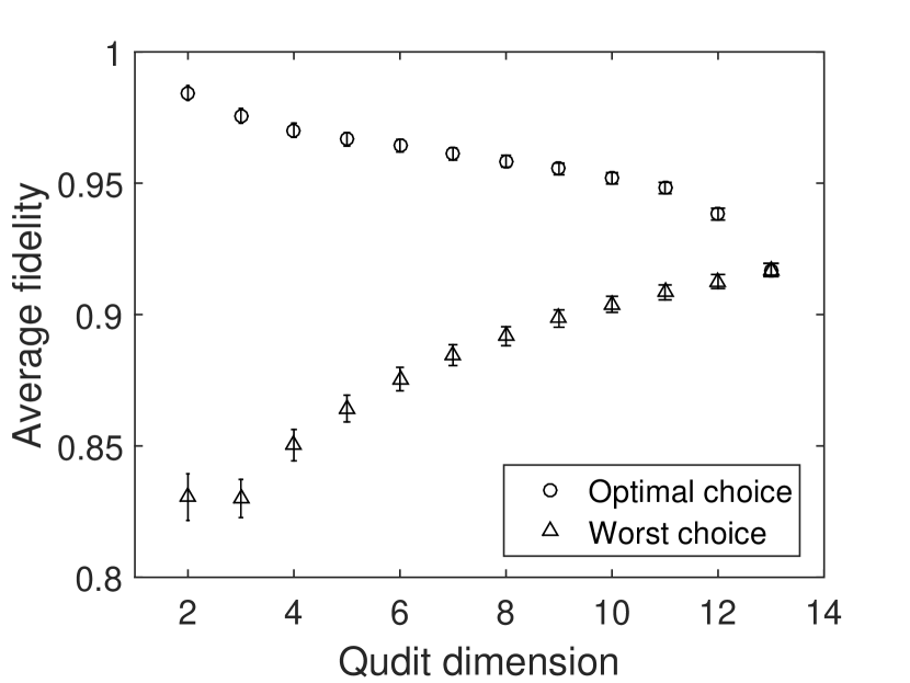
(b)

Figure 4: (a) Plot of the post-selected SPAM error for each prepared state from Fig. 3(c) against $\kappa^{2}\tau_{\pi}^{2}$, which we identify as the relevant figure of merit for errors induced by magnetic field fluctuations. $\kappa$ is the magnetic field sensitivity and $\tau_{\pi}$ is the $\pi$-pulse time. An obvious positive correlation of $\epsilon_{SPAM}$ with $\kappa^{2}\tau_{\pi}^{2}$ is observed, indicating agreement with Eq. 4. Eqs. 1 and 2 with an additional freely varying parameter for the vertical intercept are used to fit the data. (b) Scaling of average SPAM fidelity with qudit dimension, and its dependence on the choice of qudit states, computed using the data set in Fig. 3(c). For the ’optimal choice’ of qudit states, the $\lvert 6S_{1/2},F=2,m_{F}=2\rangle$ state and the $d-1$ states with the best $\pi$-pulse transition fidelities are chosen as the computational basis. For the ’worst choice’, the $d-1$ states with the worst $\pi$-pulse transition fidelities are chosen instead.

It should be noted that we have not made any efforts to mitigate magnetic field noise in this work. To reduce error from magnetic field noise, passive [28] and active [29] methods have been empirically demonstrated, with the former estimated to contribute to an error level lower than light scattering error from hyperfine Raman transitions [30]. Thus, it is expected that magnetic field noise error is not a fundamental limiting factor in the qudit protocol of this work, despite the lack of magnetically insensitive encodings for high qudit dimensions.

Another practical merit to this qudit scheme is that the calibration times of the experimental parameters (laser frequencies and $\pi$-pulse times) for SPAM do not scale with the qudit dimension with certain protocols, which are presented in Methods and Supplementary Information. Such a protocol is employed for the laser frequencies calibrations in this work. The efficient $\pi$-pulse times calibrations protocol is not used in this work due to a limitation of our experimental apparatus (see Supplementary Information).

The total measurement time of around 100 in this work is relatively long for typical trapped ion quantum operations [13]. However, this is an artificial limitation from our waveform generation methods and lack of frequency modulation for the 614 laser (see Supplementary Information for details). A fluorescence collection time of 350 has been demonstrated with ^137Ba^+ [27]. In principle, the measurement time scales linearly with qudit levels in the absence of these limitations. Thus, qudit measurement times on the order of 1 or better should be possible.

In this work, we have demonstrated high-level qudit encoding and SPAM of up to 13 levels using a ^137Ba^+ ion with an average post-selected SPAM error of $8.3\pm 0.3\%$. The major source of SPAM error in this work is magnetic field noise. However, this should not be a major roadblock for this qudit protocol, as the methods to rectify magnetic field noise are known. With improved technical control, it is possible to extend this work and encode up to 25 levels in a single ^137Ba^+ ion with good SPAM fidelities. To build a functioning quantum computer, the ability to perform single qudit gates and entangling gates are required. Such procedures have been demonstrated in Ref. [1] for a qudit dimension of 5 with ^40Ca^+, with a similar state encoding scheme and manipulation, and could be straightforwardly generalized for ^137Ba^+. Thus, our work opens prospects for a trapped-ion-based universal quantum computer with more than double the number of qudit states per ion.

Methods

^137Ba^+ Energy Levels Simulations

To calculate the energy eigenvalues and eigenstates for an arbitrary magnetic field strength, the Hamiltonian for the corresponding energy orbital is constructed in the $\lvert I,m_{I};J,m_{J}\rangle$ basis as follows

$$\hat{H} =hA_{D}\vec{I}\cdot\vec{J}$$ (5)

$$+hB_{Q}\frac{3\left(\vec{I}\cdot\vec{J}\right)^{2}+\frac{3}{2}\vec{I}\cdot\vec{J}-I\left(I+1\right)J\left(J+1\right)}{2I\left(2I-1\right)J\left(2J-1\right)}$$

$$+B_{e}\mu_{B}\left(g_{J}m_{J}+g_{I}m_{I}\right)$$

where $h$ is the Planck constant, $A_{D}$ is the magnetic dipole hyperfine structure constant, $B_{Q}$ is the electric quadrupole hyperfine structure constant, $B_{e}$ is the magnetic field strength, $\vec{I}$ and $\vec{J}$ are the nuclear and electron angular momentum vectors respectively, $I$ and $J$ are the nuclear and electron angular momentum numbers respectively, $m_{I}$ and $m_{J}$ are the projection of the nuclear and electron angular momenta along the magnetic field axis respectively, $g_{I}$ and $g_{J}$ denote the nuclear and electron g-factor respectively, and $\mu_{B}$ is the Bohr magneton. The Hamiltonian matrix is then solved numerically to obtain its eigenvalues and eigenvectors. In this work, we have set $g_{I}=0$ as it is negligible compared to $g_{J}$. For the $6S_{1/2}$ level, $A_{D}=\qty{4018.871}{\mega}$ and $B_{Q}=0$ [31]. For the $5D_{5/2}$ level, $A_{D}=\qty{-12.028}{\mega}$ and $B_{Q}=\qty{59.533}{\mega}$ [22]. With these values of the hyperfine constants for the $5D_{5/2}$ level, at a magnetic field strength of $B_{e}=\qty{8.35}{G}$, the Zeeman splitting term in Eq. 5 is comparable to the first 2 hyperfine energy splitting terms, and the $\lvert F,m_{F}\rangle$ states cease to be good approximations of the energy eigenstates of the ion. Figs. 2(a) and 2(b) show the simulation results of the energy eigenvalues and eigenvectors.

Quadrupole Transition Strength Geometric Factor

In a static magnetic field, when a quadrupole transition of $\Delta m=q$ is driven with a laser, the component of the laser field that is driving the transition can be defined by a factor $g^{(q)}\left(\gamma,\phi\right)$. The $g^{(q)}\left(\gamma,\phi\right)$ factor is dependent on the angle between the laser wavevector $\vec{k}$ and the magnetic field vector $\vec{B_{e}}$, which we define as $\phi$, and the polarization angle of the laser electric field with respect to the plane formed by $\vec{k}$ and $\vec{B_{e}}$, which we define as $\gamma$. The expressions of the $g^{(q)}\left(\gamma,\phi\right)$ factors can be derived to be [32, 33]

$$g^{(0)}\left(\gamma,\phi\right) =\frac{1}{2}|\cos\gamma\sin 2\phi|$$ (6)

$$g^{(\pm 1)}\left(\gamma,\phi\right) =\frac{1}{\sqrt{6}}|\mp\cos\gamma\cos 2\phi+i\sin\gamma\cos\phi|$$

$$g^{(\pm 2)}\left(\gamma,\phi\right) =\frac{1}{\sqrt{6}}\bigg{|}\frac{1}{2}\cos\gamma\sin 2\phi\mp i\sin\gamma\sin\phi\bigg{|}.$$

^137Ba^+ Transition Strengths in the Intermediate Magnetic Field Regime

The reduction of $6S_{1/2}\leftrightarrow 5D_{5/2}$ transition strengths for a general magnetic field strength in a linearly polarized laser perturbation can be expressed as

$$g^{(q)}\left(\gamma,\phi\right)\langle\tilde{F}_{D},m_{\tilde{F},D}\rvert\hat{Q}_{q=m_{\tilde{F},D}-m_{\tilde{F},S}}\lvert\tilde{F}_{S},m_{\tilde{F},S}\rangle$$ (7)

$$=g^{(q)}\left(\gamma,\phi\right)\langle J_{D}=5/2\rvert\lvert\hat{Q}\rvert\lvert J_{S}=1/2\rangle\langle\tilde{F}_{S},m_{\tilde{F},S};k=2,q=m_{\tilde{F},D}-m_{\tilde{F},S}\lvert\tilde{F}_{D},m_{\tilde{F},D}\rangle,$$

where the subscripts $S$ and $D$ denote the $6S_{1/2}$ and $5D_{5/2}$ levels respectively, $\hat{Q}$ is the electric quadrupole energy operator, $k=2$ is the tensor rank of the electric quadrupole energy operator, $\langle J_{D}=5/2\rvert\lvert\hat{Q}\rvert\lvert J_{S}=1/2\rangle$ is the reduced transition matrix element for the $6S_{1/2}\leftrightarrow 5D_{5/2}$ transition. The dimensionless prefactors $g^{(q)}\left(\gamma,\phi\right)\langle\tilde{F}_{S},m_{\tilde{F},S};k=2,q=m_{\tilde{F},D}-m_{\tilde{F},S}\lvert\tilde{F}_{D},m_{\tilde{F},D}\rangle$ are effectively the relative $6S_{1/2}\leftrightarrow 5D_{5/2}$ transition strengths, which are the values plotted in Fig. 2(c). The details of the calculations for the $g^{(q)}\left(\gamma,\phi\right)\langle\tilde{F}_{S},m_{\tilde{F},S};k=2,q=m_{\tilde{F},D}-m_{\tilde{F},S}\lvert\tilde{F}_{D},m_{\tilde{F},D}\rangle$ prefactors and the numerical results can be found in the Supplementary Information.

Experimental Setup

In a vacuum chamber with an air pressure of $\qty{1e{-10}}{\milli\bar{}}$, a 4-rod linear Paul trap is used to trap ^137Ba^+. Radiofrequency (RF) voltages with an estimated amplitude of $\qty{240}{}$ and a frequency of $\qty{20.772}{\mega}$ are sent to the 4-rod electrodes, with the diagonal pairs of the electrodes being out of phase with each other. Static voltages of $\qty{3}{}$ are sent to one pair of the diagonal rods to break the degeneracy of the ion radial secular motional frequencies. $\qty{10}{}$ of static voltage is applied to the needle electrodes for axial confinement. This setup results in a trapped ^137Ba^+ with radial secular motional frequencies of $\qty{1.2}{\mega}$ and $\qty{1.4}{\mega}$, and an axial motional frequency of $\qty{10}{\kilo}$.

The magnetic field orientation is as shown in Fig. 1(b). It is generated by a pair of solenoids attached to the viewports of the vacuum chamber, with an estimated magnetic field strength of $\qty{8.35}{G}$.

The $\qty{493}{\nano}$ laser is sourced from a commercial Toptica DL Pro external cavity diode laser (ECDL). An electro-optic modulator (EOM) is used to generate $\pm\qty{4012}{\mega}$ sidebands for the $\qty{493}{\nano}$ laser, where the red and blue sidebands are used to drive the $\lvert 6S_{1/2},F=2\rangle\leftrightarrow\lvert 6P_{1/2},F=2\rangle$ and $\lvert 6S_{1/2},F=1\rangle\leftrightarrow\lvert 6P_{1/2},F=2\rangle$ transitions respectively. The $\qty{493}{\nano}$ laser is split to 2 paths and sent to the trap as shown in Fig. 1(b). Each path goes through an acousto-optic modulator (AOM), which acts as a switch for the laser beam. The $\qty{493}{\nano}$ beam that is parallel to the magnetic field is circularly-polarized, $\sigma^{+}$-polarized, for optical pumping the ^137Ba^+ ion. The $\qty{493}{\nano}$ beam that is perpendicular to the magnetic field is used for cooling and fluorescent readout. This beam is linearly polarized and the polarization is tuned to maximize ion fluorescence. This beam orientation cools the ion along all three principal trap axes. The fluorescence and optical pumping $\qty{493}{\nano}$ beams have powers of $\qty{35}{\micro}$ and $\qty{6.5}{\micro}$ at the ion trap respectively. Both beams are focused to a beam diameter of approximately $\qty{70}{\micro}$ at the ion.

The $\qty{650}{\nano}$ laser is also sourced from a Toptica DL Pro ECDL. An EOM is used to generate the necessary sidebands to drive the transitions as described in Fig. 1(c) and an AOM is used as a switch for the beam going to the ion trap. The power of this beam at the trap is $\qty{230}{\micro}$ and the beam is focused down to a diameter of $\qty{70}{\micro}$ at the ion.

The $\qty{614}{\nano}$ laser is frequency doubled from a $\qty{1228}{\nano}$ laser. The $\qty{1228}{\nano}$ laser is sourced from Moglabs CEL and the frequency doubler is from NTT Electronics model WH-0614-000-F-B-C. An AOM is used as a switch for this laser. The $\qty{614}{\nano}$ laser power at the ion trap is $\qty{15}{\micro}$ and is focused down to a beam diameter of $\qty{53}{\micro}$ at the ion. The $\qty{614}{\nano}$ laser frequency is set to be resonant to the transition from the $\lvert 5D_{5/2},\tilde{F}=4,m_{\tilde{F}}=2\rangle$ state to the $\lvert 6P_{3/2},F=3\rangle$ state.

The $\qty{1762}{\nano}$ laser is from a Toptica DL Pro ECDL. The frequency stabilization system is built by Stable Laser Systems, where the laser frequency is referenced and locked to a temperature controlled Fabry–Pérot cavity in vacuum using the Pound-Drever-Hall (PDH) method. The $\qty{1762}{\nano}$ laser carrier frequency is chosen to be locked to a frequency around $\qty{600}{\mega}$ higher than the $\lvert 6S_{1/2},F=2\rangle\leftrightarrow\lvert 5D_{5/2}\rangle$ transitions. The laser is then passed through an EOM, where sideband frequencies are generated, and the red-sideband frequency is used to drive a specific chosen $\lvert 6S_{1/2},F=2\rangle\leftrightarrow\lvert 5D_{5/2}\rangle$ transition. The RF source for the $\qty{1762}{\nano}$ EOM comes from an arbitrary waveform generator (AWG), which allows us to quickly change the sideband frequency to drive the desired transitions for the SPAM process. The 1762 laser is sent to the ion from an angle that minimizes coupling to the weakly confined axial motional mode, which is $\phi=\qty{45}{}$ from the magnetic field axis. The laser power is 2.0 and is focused down to a beam diameter of 23 at the centre of the ion trap. The 1762 laser is linearly polarized and is rotated to an angle that is $\gamma=+\qty{58}{}$ from the angle that is optimal for $\Delta m=0$ transitions, in order to be able to drive $\Delta m=\pm 1$ transitions as well.

A custom-built imaging objective of numerical aperture, $NA=0.26$, is used to image the trapped ion(s). An imaging system sends the light collected from the ion to a photo-multiplier tube (PMT) which gives us the photon counts for the experiments.

Transition Frequency Calibration

The frequency calibration process employed in this work requires empirically determining $6S_{1/2}\leftrightarrow 5D_{5/2}$ transition frequencies for only 3 of the encoded states, regardless of the dimension of the qudit. The first transition frequency is the transition with the lowest magnetic field strength sensitivity, $f_{offset}$, which is the $\lvert 5D_{5/2},\tilde{F}=2,m_{\tilde{F}}=1\rangle$ state in this work. The other 2 transition frequencies are transitions with the largest magnetic fields strength sensitivity with respect to each other, $f_{low}$ and $f_{up}$, which are the $\lvert 5D_{5/2},\tilde{F}=4,m_{\tilde{F}}=-4\rangle$ and $\lvert 5D_{5/2},\tilde{F}=4,m_{\tilde{F}}=4\rangle$ states in this work. The transition frequencies for some other state $\lvert n\rangle$ encoded in the $5D_{5/2}$ level, $f_{n}$, are determined via Eq. 8,

$$f_{n}=h\left(\bm{a_{n}},\Delta f,f_{offset}\right)$$ (8)

where $\bm{a_{n}}=\left(a_{n,1},a_{n,2},\ldots a_{n,N}\right)$ is a list of parameters for the function $h\left(\bm{a_{n}},\Delta f,f_{offset}\right)$ and $\Delta f=f_{up}-f_{low}$. We find that setting $h\left(\bm{a_{n}},\Delta f,f_{offset}\right)$ as a linear function is sufficient for calibrating the transition frequencies for the drifts that we experience. So, we use

$$h\left(\bm{a_{n}},\Delta f,f_{offset}\right)=a_{n,1}\Delta f+f_{offset}+a_{n,2}.$$ (9)

The parameters $a_{n,1}$ and $a_{n,2}$ are determined from prior experiments (see Supplementary Information). In principle, it is possible to empirically determine only 2 transition frequencies, $f_{low}$ and $f_{up}$, using this technique, and set $f_{offset}=f_{low}$. This leads to a different set of parameters $\bm{a_{n}}$ that are still sufficient information to determine $f_{n}$. However, since $f_{low}$ is magnetically sensitive, it can drift during the calibration process and lead to offset errors for other calibrated frequencies $f_{n}$. Empirically, we observe that determining a transition frequency that is insensitive to magnetic field as the offset frequency, $f_{offset}$, is required for optimal results.

Experimental SPAM Procedure

The AWG waveform frequencies are calibrated to the resonant frequencies of the $\lvert 0\rangle\leftrightarrow\lvert n\neq 0\rangle$ transitions, to the precision of $\qty{1}{\kilo}$. The calibrated frequencies are then set as individual waveforms in a waveform sequence table in the AWG. A waveform in the AWG waveform sequence table repeats itself indefinitely, until an external trigger signal is sent to the AWG, which causes the AWG to switch to the subsequent waveform in the sequence table. This allows fast switching of the $\qty{1762}{\nano}$ laser frequency that is sent to the ion. Then, the pulse time required to drive a $\pi$-pulse transition for each $\lvert 0\rangle\leftrightarrow\lvert n\rangle$ transition is calibrated. The detailed methods for calibrating the AWG frequencies and $\pi$-pulse times can be found in Supplementary Information. With the AWG frequencies and $\pi$-pulse times calibrated, the pulse sequence as shown in Extended Fig. E5 is performed for collecting SPAM data. The experiment is repeated 1000 times for each prepared state to obtain a sample size of 1000.

Extended Data Figures and Tables

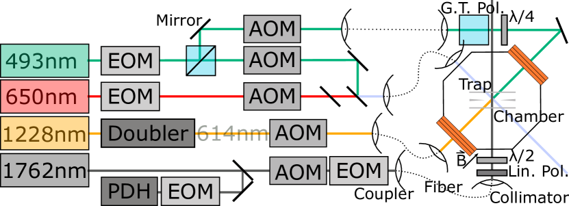
Figure E1: Detailed illustration of the optical setup used in this work. G.T. Pol. and Lin. Pol. denotes Glan-Thompson polarizer and linear polarizer respectively. $\lambda/2$ and $\lambda/4$ denote half waveplate and quarter waveplate respectively.

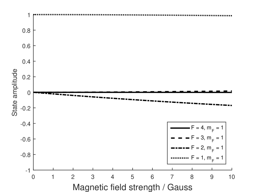
(a) $\tilde{F}=1,m_{\tilde{F}}=1$

(b) $\tilde{F}=1,m_{\tilde{F}}=0$

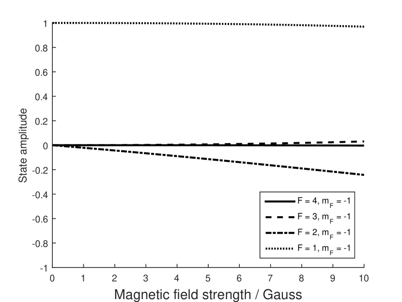
(c) $\tilde{F}=1,m_{\tilde{F}}=-1$

(d) $\tilde{F}=2,m_{\tilde{F}}=2$

(e) $\tilde{F}=2,m_{\tilde{F}}=1$

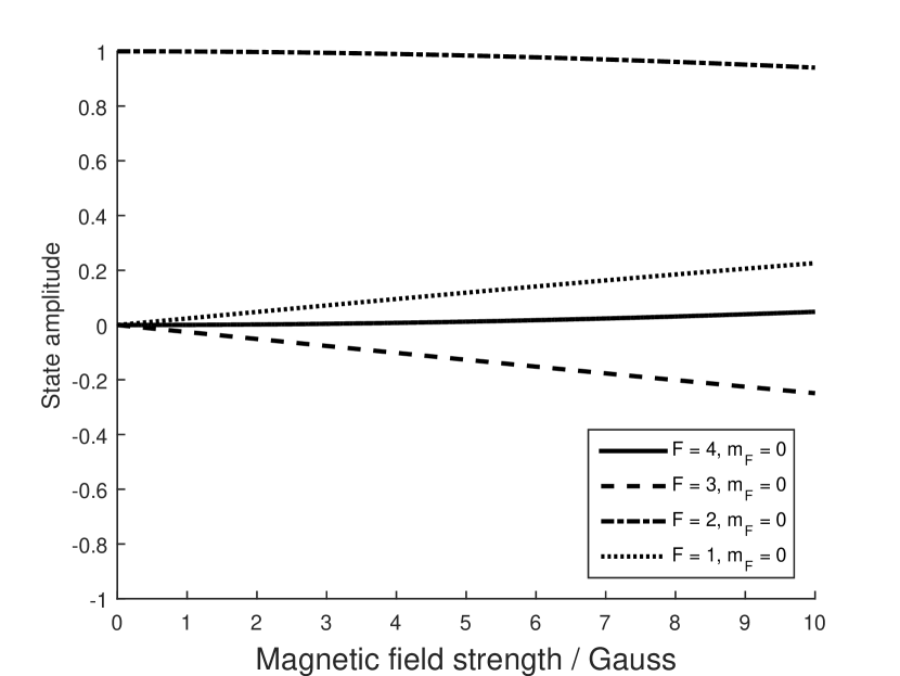
(f) $\tilde{F}=2,m_{\tilde{F}}=0$

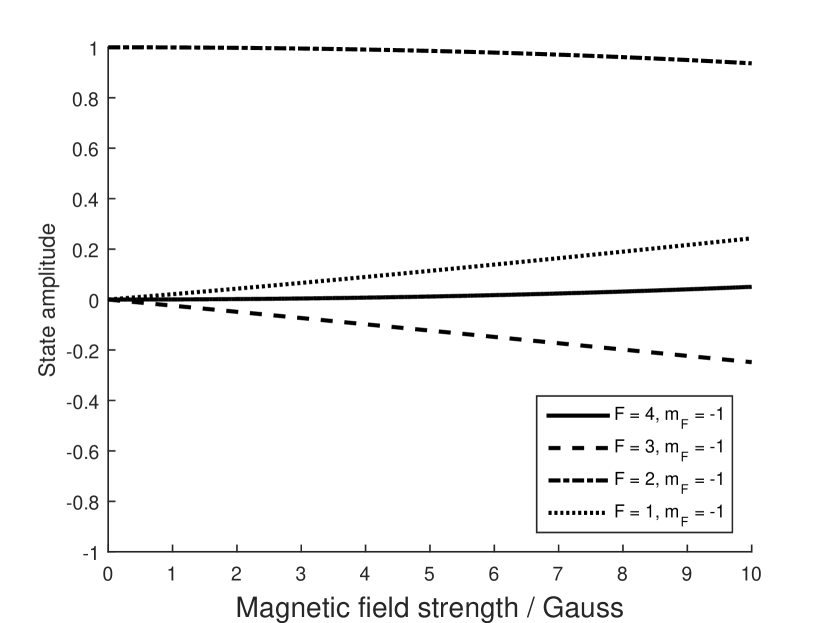
(g) $\tilde{F}=2,m_{\tilde{F}}=-1$

(h) $\tilde{F}=2,m_{\tilde{F}}=-2$

Figure E2: Numerical estimations of the ^137Ba^+ $\tilde{F}=1$ and $\tilde{F}=2$ energy eigenstates in the $5D_{5/2}$ level, expressed in the $\lvert F,m_{F}\rangle$ basis.

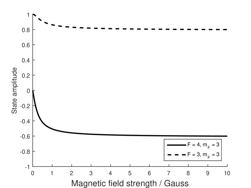
(a) $\tilde{F}=3,m_{\tilde{F}}=3$

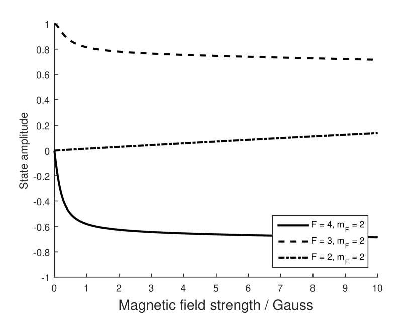
(b) $\tilde{F}=3,m_{\tilde{F}}=2$

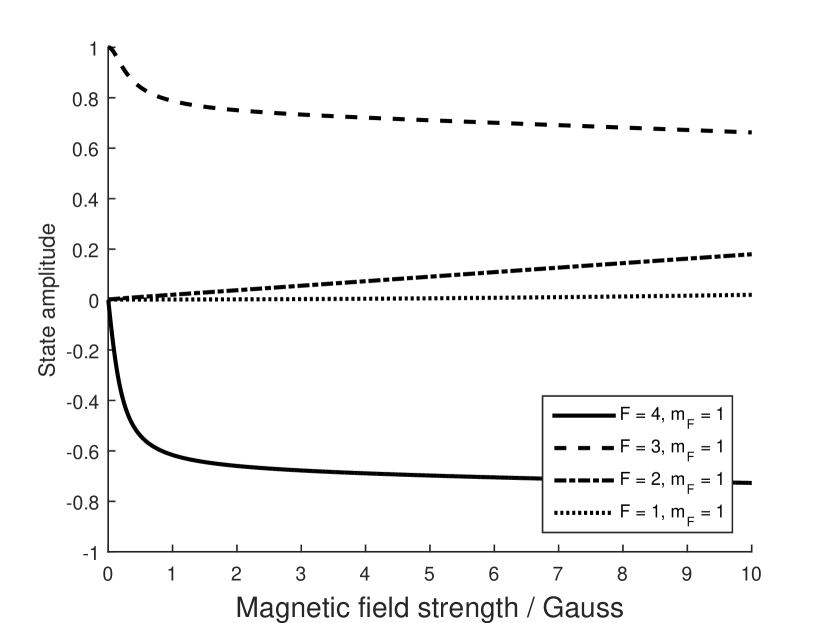
(c) $\tilde{F}=3,m_{\tilde{F}}=1$

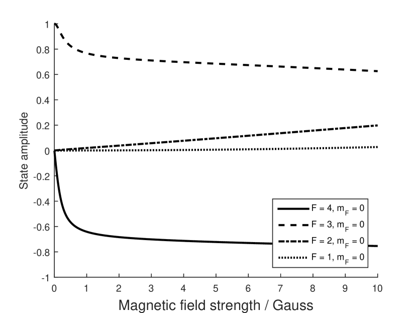
(d) $\tilde{F}=3,m_{\tilde{F}}=0$

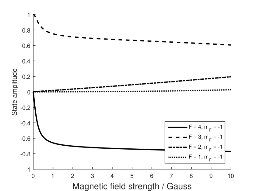
(e) $\tilde{F}=3,m_{\tilde{F}}=-1$

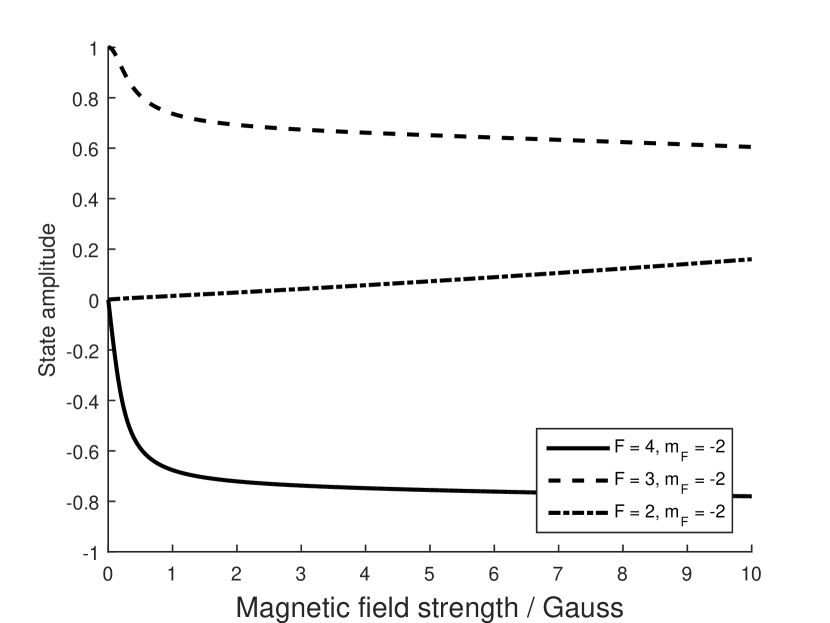
(f) $\tilde{F}=3,m_{\tilde{F}}=-2$

(g) $\tilde{F}=3,m_{\tilde{F}}=-3$

Figure E3: Numerical estimations of the ^137Ba^+ $\tilde{F}=3$ energy eigenstates in the $5D_{5/2}$ level, expressed in the $\lvert F,m_{F}\rangle$ basis.

(a) $\tilde{F}=4,m_{\tilde{F}}=4$

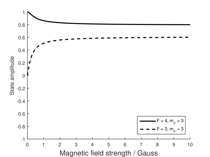
(b) $\tilde{F}=4,m_{\tilde{F}}=3$

(c) $\tilde{F}=4,m_{\tilde{F}}=2$

(d) $\tilde{F}=4,m_{\tilde{F}}=1$

(e) $\tilde{F}=4,m_{\tilde{F}}=0$

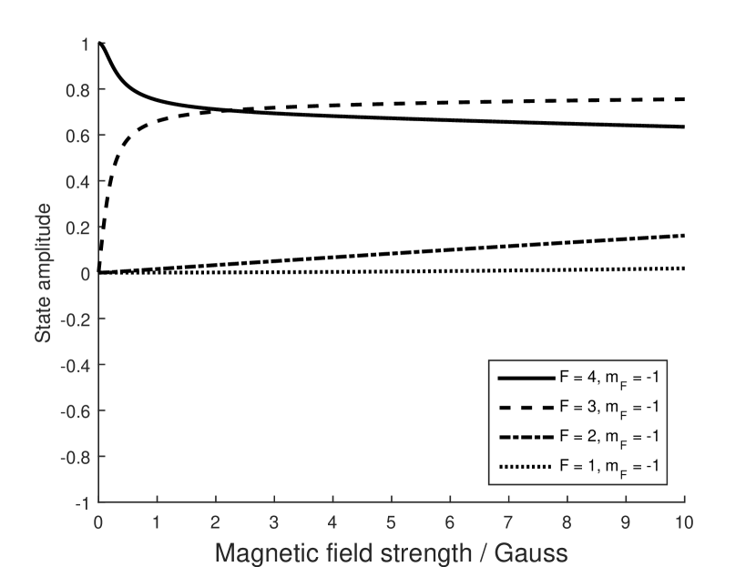
(f) $\tilde{F}=4,m_{\tilde{F}}=-1$

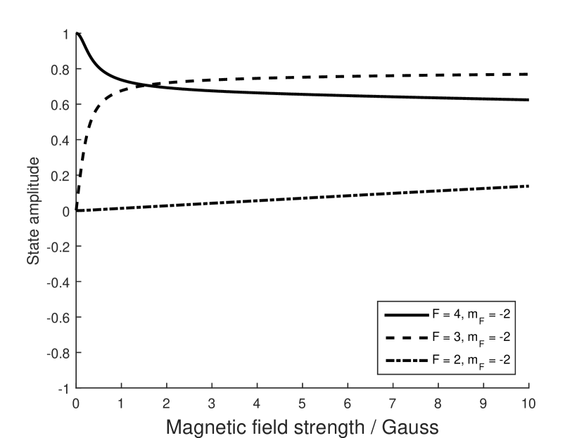
(g) $\tilde{F}=4,m_{\tilde{F}}=-2$

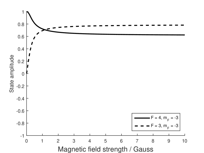
(h) $\tilde{F}=4,m_{\tilde{F}}=-3$

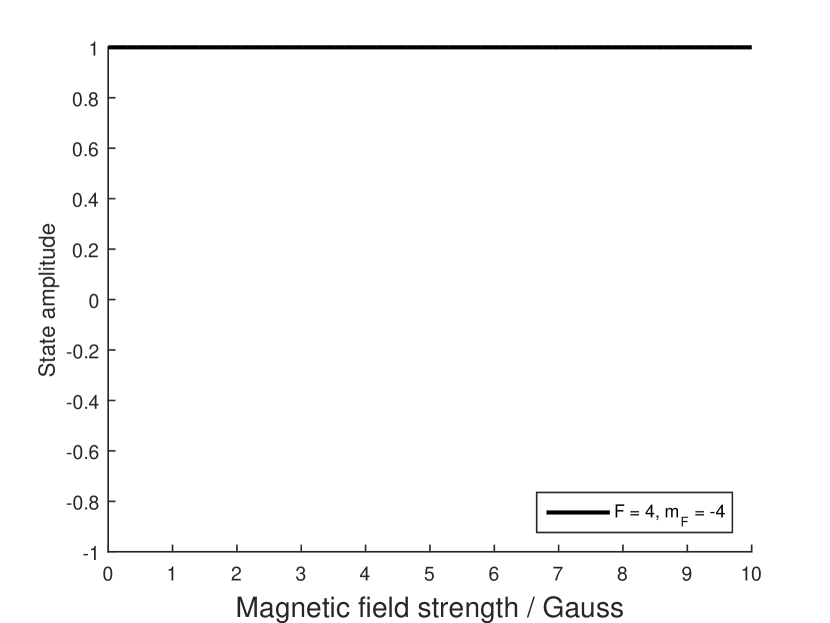
(i) $\tilde{F}=4,m_{\tilde{F}}=-4$

Figure E4: Numerical estimations of the ^137Ba^+ $\tilde{F}=4$ energy eigenstates in the $5D_{5/2}$ level, expressed in the $\lvert F,m_{F}\rangle$ basis.

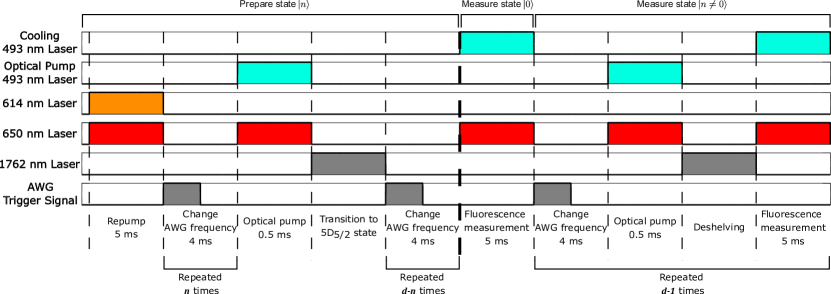
Figure E5: Pulse sequence for one SPAM experiment for a prepared $\lvert n\rangle$ state of a $d$-dimensional qudit demonstrated in this work. The first five rows denote the on/off states of the laser beams as described in text. The last row denotes an electrical signal sent to the AWG to trigger the switch to the next waveform, effectively changing the frequency of the 1762 laser. The time axis is not drawn to scale. The pulse sequences to the left and right of the bold dashed line are the state preparation and state measurement processes respectively. A list of $d$ individual frequencies corresponding to the transitions for each encoded state in a $d$-dimensional qudit is set in the AWG, and frequency switching is achieved by the AWG trigger signal. For state $\lvert 0\rangle$, the AWG frequency is set to a frequency that is off-resonant to any of the $6S_{1/2}\leftrightarrow 5D_{5/2}$ transitions. The optical pumping step in the measurement process is technically unnecessary for the measurement procedure described in the main text. It is present in this work for investigating another method of determining a measured state, which we have found to be less robust than what is described in the main text (see Supplementary Information).

$5D_{5/2}$ state	$6S_{1/2}$ state
	$\tilde{F}=1$			$\tilde{F}=2$
	$m_{\tilde{F}}=-1$	$m_{\tilde{F}}=0$	$m_{\tilde{F}}=1$	$m_{\tilde{F}}=-2$	$m_{\tilde{F}}=-1$	$m_{\tilde{F}}=0$	$m_{\tilde{F}}=1$	$m_{\tilde{F}}=2$
$\tilde{F}=1,m_{\tilde{F}}=1$	0.2139	0.1121	0.0569	0	0.0532	0.0462	0.0388	0.0226
$\tilde{F}=1,m_{\tilde{F}}=0$	0.1540	0.1535	0.0982	0.0689	0.0145	0.0149	0.0289	0.0386*
$\tilde{F}=1,m_{\tilde{F}}=-1$	0.1114	0.1390	0.1679	0.0537	0.0504	0.0327	0.0200	0
$\tilde{F}=2,m_{\tilde{F}}=2$	0	0.1948	0.0988	0	0	0.1010	0.0838	0.0581*
$\tilde{F}=2,m_{\tilde{F}}=1$	0.1049	0.1211	0.1437	0	0.1112	0.0080	0.0571	0.0724*
$\tilde{F}=2,m_{\tilde{F}}=0$	0.1287	0.0579	0.1487	0.0796	0.0683	0.0678	0.0083	0.0727*
$\tilde{F}=2,m_{\tilde{F}}=-1$	0.1562	0.0312	0.1540	0.1009	0.0028	0.0548	0.0782	0
$\tilde{F}=2,m_{\tilde{F}}=-2$	0.1382	0.1634	0	0.1046	0.0813	0.0551	0	0
$\tilde{F}=3,m_{\tilde{F}}=3$	0	0	0.1352	0	0	0	0.2309	0.0036
$\tilde{F}=3,m_{\tilde{F}}=2$	0	0.0493	0.1054	0	0	0.1813	0.1359	0.0312*
$\tilde{F}=3,m_{\tilde{F}}=1$	0.0127	0.0622	0.0965	0	0.1145	0.1777	0.0690	0.0371*
$\tilde{F}=3,m_{\tilde{F}}=0$	0.0232	0.0807	0.0709	0.0543	0.1584	0.1544	0.0043	0.0324*
$\tilde{F}=3,m_{\tilde{F}}=-1$	0.0426	0.0819	0.0516	0.1016	0.1952	0.0756	0.0326	0
$\tilde{F}=3,m_{\tilde{F}}=-2$	0.0630	0.0843	0	0.1749	0.1545	0.0052	0	0
$\tilde{F}=3,m_{\tilde{F}}=-3$	0.1058	0	0	0.2189	0.0561	0	0	0
$\tilde{F}=4,m_{\tilde{F}}=4$	0	0	0	0	0	0	0	0.2676*
$\tilde{F}=4,m_{\tilde{F}}=3$	0	0	0.1015	0	0	0	0.0636	0.2189*
$\tilde{F}=4,m_{\tilde{F}}=2$	0	0.0503	0.0952	0	0	0.0011	0.1285	0.1943*
$\tilde{F}=4,m_{\tilde{F}}=1$	0.0176	0.0694	0.0945	0	0.0200	0.0472	0.1805	0.1298*
$\tilde{F}=4,m_{\tilde{F}}=0$	0.0330	0.0933	0.0721	0.0169	0.0049	0.1161	0.1703	0.0806*
$\tilde{F}=4,m_{\tilde{F}}=-1$	0.0593	0.0949	0.0532	0.0241	0.0385	0.1617	0.1450	0
$\tilde{F}=4,m_{\tilde{F}}=-2$	0.0831	0.0963	0	0.0243	0.1070	0.1996	0	0
$\tilde{F}=4,m_{\tilde{F}}=-3$	0.1323	0	0	0.0037	0.2326	0	0	0
$\tilde{F}=4,m_{\tilde{F}}=-4$	0	0	0	0.2676	0	0	0	0

Table E1: Relative transition strength factors $\langle\tilde{F}_{S},m_{\tilde{F},S};k=2,q=m_{\tilde{F},D}-m_{\tilde{F},S}\lvert\tilde{F}_{D},m_{\tilde{F},D}\rangle$ for $6S_{1/2}\leftrightarrow 5D_{5/2}$ transitions with $\phi=\qty{45}{}$ and $\gamma=\qty{58}{}$ at a magnetic field strength of $\qty{8.35}{G}$. Values higher than $0.03$ are in bold texts. The value of 0.03 is determined by empirically observing that the transitions weaker than this have large errors due to decoherence from the SPAM experiments in this work, which is also a value that is approximately an order of magnitude lower than the strongest transitions. *Transitions used in this work.

Prepared state	Measured state
	$\lvert 0\rangle$	$\lvert 1\rangle$	$\lvert 2\rangle$	$\lvert 3\rangle$	$\lvert 4\rangle$	$\lvert 5\rangle$	$\lvert 6\rangle$	$\lvert 7\rangle$	$\lvert 8\rangle$	$\lvert 9\rangle$	$\lvert 10\rangle$	$\lvert 11\rangle$	$\lvert 12\rangle$
$\lvert 0\rangle$	0.999	0.001	0	0	0	0	0	0	0	0	0	0	0
$\lvert 1\rangle$	0.061	0.939	0	0	0	0	0	0	0	0	0	0	0
$\lvert 2\rangle$	0.038	0.001	0.958	0.001	0	0	0.002	0	0	0	0	0	0
$\lvert 3\rangle$	0.029	0.001	0	0.970	0	0	0	0	0	0	0	0	0
$\lvert 4\rangle$	0.045	0	0	0	0.953	0	0	0	0	0	0	0	0
$\lvert 5\rangle$	0.087	0.001	0	0	0	0.911	0	0	0.001	0	0	0	0
$\lvert 6\rangle$	0.318	0.001	0.003	0.003	0.003	0.001	0.662	0.003	0.001	0.001	0	0.004	0.001
$\lvert 7\rangle$	0.061	0	0.002	0	0	0.001	0.004	0.932	0	0	0	0	0
$\lvert 8\rangle$	0.076	0	0	0.001	0	0	0.002	0	0.920	0	0	0.001	0
$\lvert 9\rangle$	0.145	0.002	0	0.003	0.001	0.005	0.003	0.002	0.001	0.829	0.007	0	0.001
$\lvert 10\rangle$	0.029	0.003	0.002	0	0.001	0.003	0.003	0.002	0	0.002	0.952	0	0.002
$\lvert 11\rangle$	0.039	0.002	0.003	0.001	0.001	0.001	0.001	0.004	0	0.004	0	0.942	0.001
$\lvert 12\rangle$	0.044	0.001	0	0	0	0	0	0	0	0.001	0	0	0.954

Table E2: Post-selected measurement probability of each prepared state from SPAM experiments used to plot Fig. 3(c). See Extended Data Table E3 for the raw measurement probabilities.

Prepared state	Measured state
	$\lvert 0\rangle$	$\lvert 1\rangle$	$\lvert 2\rangle$	$\lvert 3\rangle$	$\lvert 4\rangle$	$\lvert 5\rangle$	$\lvert 6\rangle$	$\lvert 7\rangle$	$\lvert 8\rangle$	$\lvert 9\rangle$	$\lvert 10\rangle$	$\lvert 11\rangle$	$\lvert 12\rangle$	Null
$\lvert 0\rangle$	0.999	0.001	0	0	0	0	0	0	0	0	0	0	0	0
$\lvert 1\rangle$	0.059	0.911	0	0	0	0	0	0	0	0	0	0	0	0.030
$\lvert 2\rangle$	0.037	0.001	0.941	0.001	0	0	0.002	0	0	0	0	0	0	0.018
$\lvert 3\rangle$	0.029	0.001	0	0.960	0	0	0	0	0	0	0	0	0	0.010
$\lvert 4\rangle$	0.044	0	0	0	0.926	0	0	0	0.002	0	0	0	0	0.028
$\lvert 5\rangle$	0.080	0.001	0	0	0	0.841	0	0	0	0.001	0	0	0	0.077
$\lvert 6\rangle$	0.252	0.001	0.002	0.002	0.002	0.001	0.525	0.002	0.001	0.001	0	0.003	0.001	0.207
$\lvert 7\rangle$	0.058	0	0.002	0	0	0.001	0.004	0.887	0	0	0	0	0	0.048
$\lvert 8\rangle$	0.071	0	0	0.001	0	0	0.002	0	0.861	0	0	0.001	0	0.064
$\lvert 9\rangle$	0.126	0.002	0	0.003	0.001	0.004	0.003	0.002	0.001	0.722	0.006	0	0.001	0.129
$\lvert 10\rangle$	0.027	0.003	0.002	0	0.001	0.003	0.003	0.002	0	0.002	0.897	0	0.002	0.058
$\lvert 11\rangle$	0.037	0.002	0.003	0.001	0.001	0.001	0.001	0.004	0	0.004	0	0.897	0.001	0.049
$\lvert 12\rangle$	0.043	0.001	0	0	0	0	0	0	0	0.001	0	0	0.929	0.026

Table E3: Raw measurement probability of each prepared state from SPAM experiments. The sample size is $1000$. Null indicates that all fluorescence readouts during the measurement procedure are dark and no valid computational state output is obtained.

Computational state	Atomic State	SPAM error	Relative magnetic field sensitivity /   G^-1	$\pi$-pulse time, $\tau_{\pi}$ /	Estimated single transition error
$\lvert 0\rangle$	$\lvert 6S_{1/2},\tilde{F}=2,m_{\tilde{F}}=2\rangle$	$0.001$	NA	NA	NA
$\lvert 1\rangle$	$\lvert 5D_{5/2},\tilde{F}=4,m_{\tilde{F}}=4\rangle$	$0.061$	$2.7992$	$37.2$	$0.075$
$\lvert 2\rangle$	$\lvert 5D_{5/2},\tilde{F}=4,m_{\tilde{F}}=3\rangle$	$0.042$	$1.1202$	$29.7$	$0.016$
$\lvert 3\rangle$	$\lvert 5D_{5/2},\tilde{F}=4,m_{\tilde{F}}=2\rangle$	$0.030$	$-0.3554$	$37.5$	$0.023$
$\lvert 4\rangle$	$\lvert 5D_{5/2},\tilde{F}=4,m_{\tilde{F}}=1\rangle$	$0.047$	$-1.7009$	$54.9$	$0.030$
$\lvert 5\rangle$	$\lvert 5D_{5/2},\tilde{F}=4,m_{\tilde{F}}=0\rangle$	$0.09$	$-2.9234$	$63.0$	$0.07$
$\lvert 6\rangle$	$\lvert 5D_{5/2},\tilde{F}=3,m_{\tilde{F}}=2\rangle$	$0.34$	$1.7050$	$204.8$	$0.23$
$\lvert 7\rangle$	$\lvert 5D_{5/2},\tilde{F}=3,m_{\tilde{F}}=1\rangle$	$0.068$	$0.5718$	$188.3$	$0.050$
$\lvert 8\rangle$	$\lvert 5D_{5/2},\tilde{F}=3,m_{\tilde{F}}=0\rangle$	$0.080$	$-0.5672$	$151.2$	$0.049$
$\lvert 9\rangle$	$\lvert 5D_{5/2},\tilde{F}=2,m_{\tilde{F}}=2\rangle$	$0.17$	$2.0094$	$104.5$	$0.11$
$\lvert 10\rangle$	$\lvert 5D_{5/2},\tilde{F}=2,m_{\tilde{F}}=1\rangle$	$0.047$	$0.3026$	$87.3$	$0.030$
$\lvert 11\rangle$	$\lvert 5D_{5/2},\tilde{F}=2,m_{\tilde{F}}=0\rangle$	$0.058$	$-1.3707$	$64.1$	$0.026$
$\lvert 12\rangle$	$\lvert 5D_{5/2},\tilde{F}=1,m_{\tilde{F}}=0\rangle$	$0.046$	$-0.7373$	$105.4$	$0.054$
NA	$\lvert 5D_{5/2},\tilde{F}=1,m_{\tilde{F}}=1\rangle$	NA	$1.9462$	$215$	$0.31$
NA	$\lvert 5D_{5/2},\tilde{F}=3,m_{\tilde{F}}=3\rangle$	NA	$2.7988$	$\sim 2000$*	NA

Table E4: Table summarizing the encoded states and their corresponding physical atomic states, parameters relevant to the SPAM experiments and post-selected SPAM errors. See Supplementary Information for how the single transition errors are estimated. *This value is estimated from relative transition strengths using Table E1, and not measured empirically.

Acknowledgements

We thank Yvette de Sereville for assisting with preliminary calibrations, and we thank Nicholas Zutt and Noah Greenberg for reviewing the manuscript. This research was supported, in part, by the Natural Sciences and Engineering Research Council of Canada (NSERC), RGPIN-2018-05253 and the Canada First Research Excellence Fund (CFREF) (Transformative Quantum Technologies), CFREF-2015-00011. C.S. is also supported by a Canada Research Chair.

Author contributions statement

P.J.L., B.W. and C.S. conceived the experiment(s), P.J.L. and B.W. conducted the experiment(s), P.J.L., B.W. and C.S. analyzed the results. All authors reviewed the manuscript.

Additional information

The authors report no competing interests in the submission of this article.

References

- [1] Ringbauer, M. et al. A universal qudit quantum processor with trapped ions. \JournalTitleNature Physics 18, 1053–1057, DOI: 10.1038/s41567-022-01658-0 (2022).
- [2] Campbell, E. T., Anwar, H. & Browne, D. E. Magic-state distillation in all prime dimensions using quantum Reed-Muller codes. \JournalTitlePhys. Rev. X 2, 041021, DOI: 10.1103/PhysRevX.2.041021 (2012).
- [3] Campbell, E. T. Enhanced fault-tolerant quantum computing in d-Level systems. \JournalTitlePhys. Rev. Lett. 113, 230501, DOI: 10.1103/PhysRevLett.113.230501 (2014).
- [4] Andrist, R. S., Wootton, J. R. & Katzgraber, H. G. Error thresholds for Abelian quantum double models: Increasing the bit-flip stability of topological quantum memory. \JournalTitlePhys. Rev. A 91, 042331, DOI: 10.1103/PhysRevA.91.042331 (2015).
- [5] Hutter, A., Loss, D. & Wootton, J. R. Improved hdrg decoders for qudit and non-abelian quantum error correction. \JournalTitleNew Journal of Physics 17, 035017, DOI: 10.1088/1367-2630/17/3/035017 (2015).
- [6] Watson, F. H. E., Anwar, H. & Browne, D. E. Fast fault-tolerant decoder for qubit and qudit surface codes. \JournalTitlePhys. Rev. A 92, 032309, DOI: 10.1103/PhysRevA.92.032309 (2015).
- [7] Senko, C. et al. Realization of a quantum integer-spin chain with controllable interactions. \JournalTitlePhys. Rev. X 5, 021026, DOI: 10.1103/PhysRevX.5.021026 (2015).
- [8] et al., B. A. Engineering an effective three-spin hamiltonian in trapped-ion systems for applications in quantum simulation. \JournalTitleQuantum Sci. Technol. 7 034001 DOI: 10.1088/2058-9565/ac5f5b (2022).
- [9] Lanyon, B. P. et al. Simplifying quantum logic using higher-dimensional Hilbert spaces. \JournalTitleNature Phys. 5, 134–140, DOI: 10.1038/nphys1150 (2008).
- [10] Ralph, T. C., Resch, K. J. & Gilchrist, A. Efficient Toffoli gates using qudits. \JournalTitlePhys. Rev. A 75, 022313, DOI: 10.1103/PhysRevA.75.022313 (2007).
- [11] Ladd, T. D. et al. Quantum computers. \JournalTitleNature 464, 45–53, DOI: 10.1038/nature08812 (2010).
- [12] Bruzewicz, C. D., Chiaverini, J., McConnell, R. & Sage, J. M. Trapped-ion quantum computing: Progress and challenges. \JournalTitleApplied Physics Reviews 6, 021314, DOI: 10.1063/1.5088164 (2019). https://doi.org/10.1063/1.5088164.
- [13] Gaebler, J. P. et al. High-fidelity universal gate set for ion qubits. \JournalTitlePhys. Rev. Lett. 117, 060505, DOI: 10.1103/PhysRevLett.117.060505 (2016).
- [14] Philips, S. G. J. et al. Universal control of a six-qubit quantum processor in silicon. \JournalTitleNature 609, 919–924, DOI: 10.1038/s41586-022-05117-x (2022).
- [15] Kielpinski, D., Monroe, C. & Wineland, D. J. Architecture for a large-scale ion-trap quantum computer. \JournalTitleNature 417, 709–711, DOI: 10.1038/nature00784 (2002).
- [16] Monroe, C. et al. Large-scale modular quantum-computer architecture with atomic memory and photonic interconnects. \JournalTitlePhys. Rev. A 89, 022317, DOI: 10.1103/PhysRevA.89.022317 (2014).
- [17] Smith, A. et al. Quantum control in the cs ground manifold using radio-frequency and microwave magnetic fields. \JournalTitlePhys. Rev. Lett. 111, 170502, DOI: 10.1103/PhysRevLett.111.170502 (2013).
- [18] Leupold, F. M. et al. Sustained state-independent quantum contextual correlations from a single ion. \JournalTitlePhys. Rev. Lett. 120, 180401, DOI: 10.1103/PhysRevLett.120.180401 (2018).
- [19] Malinowski, M. et al. Probing the limits of correlations in an indivisible quantum system. \JournalTitlePhys. Rev. A 98, 050102, DOI: 10.1103/PhysRevA.98.050102 (2018).
- [20] Hrmo, P. et al. Native qudit entanglement in a trapped ion quantum processor. \JournalTitleNature Communications 14, 2242, DOI: 10.1038/s41467-023-37375-2 (2023).
- [21] Madej, A. A. & Sankey, J. D. Quantum jumps and the single trapped barium ion: Determination of collisional quenching rates for the 5 level. \JournalTitlePhys. Rev. A 41, 2621–2630, DOI: 10.1103/PhysRevA.41.2621 (1990).
- [22] Silverans, R. E., Borghs, G., De Bisschop, P. & Van Hove, M. Hyperfine structure of the 5d states in the alkaline-earth ba ion by fast-ion-beam laser-rf spectroscopy. \JournalTitlePhys. Rev. A 33, 2117–2120, DOI: 10.1103/PhysRevA.33.2117 (1986).
- [23] Berkeland, D. J. & Boshier, M. G. Destabilization of dark states and optical spectroscopy in zeeman-degenerate atomic systems. \JournalTitlePhys. Rev. A 65, 033413, DOI: 10.1103/PhysRevA.65.033413 (2002).
- [24] Qudit 13level spam scripts and data. https://doi.org/10.5281/zenodo.8000676 (2023).
- [25] Ball, H. & Biercuk, M. J. Walsh-synthesized noise filters for quantum logic. \JournalTitleEPJ Quantum Technology 2, 11, DOI: 10.1140/epjqt/s40507-015-0022-4 (2015).
- [26] Day, M. L., Low, P. J., White, B., Islam, R. & Senko, C. Limits on atomic qubit control from laser noise. \JournalTitlenpj Quantum Information 8, 72, DOI: 10.1038/s41534-022-00586-4 (2022).
- [27] An, F. A. et al. High fidelity state preparation and measurement of ion hyperfine qubits with . \JournalTitlePhys. Rev. Lett. 129, 130501, DOI: 10.1103/PhysRevLett.129.130501 (2022).
- [28] Ruster, T. et al. A long-lived zeeman trapped-ion qubit. \JournalTitleApplied Physics B 122, 254, DOI: 10.1007/s00340-016-6527-4 (2016).
- [29] Hu, H., Xie, Y. & chao Zhang et al., M. Compensation of low-frequency noise induced by power line in trapped-ion system. \JournalTitlePREPRINT (Version 1) available at Research Square DOI: 10.21203/rs.3.rs-1608974/v1 (2022).
- [30] Low, P. J., White, B. M., Cox, A. A., Day, M. L. & Senko, C. Practical trapped-ion protocols for universal qudit-based quantum computing. \JournalTitlePhys. Rev. Res. 2, 033128, DOI: 10.1103/PhysRevResearch.2.033128 (2020).
- [31] Blatt, R. & Werth, G. Precision determination of the ground-state hyperfine splitting in using the ion-storage technique. \JournalTitlePhys. Rev. A 25, 1476–1482, DOI: 10.1103/PhysRevA.25.1476 (1982).
- [32] Roos, C. Controlling the quantum state of trapped ions. PhD dissertation, University of Innsbruck (2000). Available at https://www.quantumoptics.at/images/publications/dissertation/roos-diss.pdf.
- [33] Bramman, B. Measuring Trapped Ion Qudits. MSc thesis, University of Waterloo (2019). Available at https://uwspace.uwaterloo.ca/handle/10012/15165.