Impact of Bending Stiffness on Ground-state Conformations for Semiflexible Polymers

Abstract

Many variants of RNA, DNA, even proteins can be considered semiflexible polymers, where bending stiffness, as a type of energetic penalty, competes with attractive van der Waals forces in structure formation processes. Here, we systematically investigate the effect of the bending stiffness on ground-state conformations of a generic coarse-grained model for semiflexible polymers. This model possesses multiple transition barriers. Therefore, we employ advanced generalized-ensemble Monte Carlo methods to search for the lowest-energy conformations. As the formation of distinct versatile ground-state conformations including compact globules, rod-like bundles and toroids strongly depends on the strength of the bending restraint, we also performed a detailed analysis of contact and distance maps.

I Introduction

Biomolecules form distinct structures that allow them to perform specific functions in the physiological environment. Understanding the effects of different properties of these conformations is crucial in many fields, such as disease studies Sagis2004 and drug design drug2020 . With the recent development of computational resources and algorithms, computer simulations have become one of the most powerful tools for studies of macromolecular structures. However, atomistic or quantum level modeling is still limited by the computational power needed to properly describe complex electron distributions in the system, not to mention the thousands of “force field” parameters to be tuned in semiclassical models quantum2019 ; Atomic2011 ; Bachmann2014Book . Moreover, such models are so specific that their results usually lack generality. Thus, coarse-grained polymer models have been widely used in recent years. Focusing on few main features, while other less relevant degrees of freedom are considered averaged out, provides a more general view at generic structural properties of polymers.

Semiflexible polymer models play an important role as they allow for studies of various classes of biopolymers daniel2013 ; Janke2015 ; Chen2018 ; Majumder21 ; Shirts2022 , for which the bending stiffness is known to be one of the key factors to be reckoned with in structure formation processes. Bending restraints help DNA strands fold in an organized way enabling efficient translation and transcription processes DNApacking . RNA stiffness affects self-assembly of virus particles RNAstiff2018 . In addition, protein stiffness has been found to be an important aspect in enzymatic catalysis processes, where proteins increase stiffness to enhance efficiency ProteinStiff2019 .

The well-known Kratky-Porod or worm-like chain (WLC) model WLC has frequently been used in studies of basic structural and dynamic properties of semiflexible polymers. However, lack of self-interactions in this model prevents structural transitions. In this paper, we systematically study the competition between attractive interactions, which usually are caused by hydrophobic van der Waals effects in solvent, and the impact of the bending stiffness for ground-state conformations of a coarse-grained model for semiflexible polymers by means of advanced Monte Carlo (MC) simulations.

Our study helps identify the conditions which allow semiflexible polymers to form distinct geometric structures closely knitted to their biological function. For example, sufficient bending strength of the polymer chain is necessary for the formation of toroidal shapes. Such conformations are relevant for stable DNA-protein complexes bustamante1 ; kulic1 . Also, DNA spooled into virus capsids tends to form toroidal structures, which support both optimal accommodation of DNA in a tight environment and the fast release due to the tension built up inside the capsid linse1 ; cb1 .

The paper is organized as follows: Semiflexible polymer model and simulation methods are introduced in Sec. II. Results of energetic and structural analyses of lowest-energy conformations are discussed in Sec. III. The summary in Sec. IV concludes the paper.

II Model and Methods

Table 1: Lowest-energy conformations and corresponding energy values obtained from simulations for the selected values of the bending stiffness ranging from $\kappa=0$ (fully flexible) to $\kappa=19$.

II.1 Coarse-grained model for semiflexible polymers

In a generic coarse-grained model for linear homopolymers, the monomers are identical and connected by elastic bonds. Three energetic contributions are considered in the model used in our study: bonded interactions, non-bonded interactions and energetic penalty due to bending stiffness. The interaction between non-bonded monomers, which depends on the monomer-monomer distance $r$,

$$V_{\mathrm{NB}}(r)=\begin{cases}V_{\mathrm{LJ}}(r)-V_{\mathrm{shift}},&r<r_{c},\\ 0,&\text{otherwise,}\end{cases}$$ (1)

is governed by the standard 12-6 Lennard-Jones (LJ) potential

$$V_{\mathrm{LJ}}(r)=4\epsilon_{\mathrm{LJ}}\left[\left(\dfrac{\sigma}{r}\right)^{12}-\left(\dfrac{\sigma}{r}\right)^{6}\right].$$ (2)

The energy scale is fixed by $\epsilon_{\mathrm{LJ}}$. The potential minimum is located at $r_{0}=2^{1/6}\sigma$, where $\sigma$ is the van der Waals radius. A cutoff at $r_{c}=2.5\sigma$ is applied to reduce computational cost and the potential is shifted by a constant $V_{\mathrm{shift}}\equiv V_{\mathrm{LJ}}(r_{c})$ to avoid a discontinuity.

The bond elasticity between adjacent monomers is described by the combination of Lennard-Jones and finitely extensible nonlinear elastic (FENE) potentials Milchev2001 ; Kremer1990 ; Bird1987 , with the minimum located at $r_{0}$:

$$V_{\mathrm{B}}(r)=-\frac{1}{2}KR^{2}\mathrm{ln}\left[1-\left(\frac{r-r_{0}}{R}\right)^{2}\right]+V_{\mathrm{LJ}}(r)-V_{\mathrm{shift}}.$$ (3)

Here, the standard values $R=(3/7)r_{0}$ and $K=(98/5)\epsilon_{\mathrm{LJ}}r_{0}^{2}$ are used Qi2014 . Due to bond rigidity, the fluctuations of the bond length $r$ are limited to the range $[r_{0}-R,r_{0}+R]$.

To model the impact of chain rigidity, a bending potential is introduced. The energetic penalty accounts for the deviation of the bond angle $\theta$ from the reference angle $\theta_{0}$ between neighboring bonds:

$$V_{\mathrm{bend}}(\theta)=\kappa\left[1-\cos(\theta-\theta_{0})\right],$$ (4)

where $\kappa$ is the bending stiffness parameter. In this study we set $\theta_{0}=0$.

Eventually, the total energy of a polymer chain with conformation $\bm{X}=\left(\bm{r}_{1},...,\bm{r}_{N}\right)$ is given by

$$E(\bm{X})=\sum_{i>j+1}V_{\mathrm{NB}}(r_{i,j})+\sum_{i}V_{\mathrm{B}}(r_{i,i+1})+\sum_{l}V_{\mathrm{bend}}(\theta_{l}),$$ (5)

where $r_{i,j}=|\bm{r}_{i}-\bm{r}_{j}|$ represents the distance between monomers at positions $\bm{r}_{i}$ and $\bm{r}_{j}$.

The length scale $r_{0}$, the energy scale $\epsilon_{\mathrm{LJ}}$, as well as the Boltzmann constant $k_{\mathrm{B}}$ are set to unity in our simulations. The polymer chain consists of $N=55$ monomers aierken20 .

II.2 Stochastic Sampling Methods

The model we have studied has a complex hyperphase diagram that exhibits a multitude of structural phases. Crossing the transition lines separating these phases in the search for ground-state conformations is a challenging task. Advanced generalized-ensemble Monte Carlo (MC) techniques have been developed to cover the entire energy range of a system, including the lowest-energy states. In this study, we primarily used the replica-exchange Monte Carlo method (parallel tempering) Swendsen1986 ; Geyer1991 ; Hukushima1996_Japan ; Hukushima1996 ; Earl2005 and an extended two-dimensional version of it Majumder21 with advanced MC update strategies.

In each parallel tempering simulation thread $k$, Metropolis Monte Carlo simulations are performed. The Metropolis acceptance probability that satisfies detailed balance is generally written as:

$$a(\bm{X}\to\bm{X}^{\prime})=\mathrm{min}\left(\sigma(\bm{X},\bm{X}^{\prime})\omega(\bm{X},\bm{X}^{\prime}),1\right),$$ (6)

where $\omega(\bm{X},\bm{X}^{\prime})=\exp\left(-(E(\bm{X}^{\prime})-E(\bm{X}))/k_{\mathrm{B}}T_{k}\right)$ is the ratio of microstate probabilities at temperature $T_{k}$, and $\sigma(\bm{X},\bm{X^{\prime}})=s\left(\bm{X^{\prime}\to X}\right)/s\left(\bm{X\to X^{\prime}}\right)$ is the ratio of forward and backward selection probabilities for specific updates. Replicas with the total energy $E_{k}$ and $E_{k+1}$ are exchanged between adjacent threads $k$ and $k+1$ with the standard exchange acceptance probability:

$$P=\mathrm{min}\left(\exp\left[\left(\beta_{k}-\beta_{k+1}\right)\left(E_{k}-E_{k+1}\right)\right],1\right),$$ (7)

where $\beta_{k}=(k_{\mathrm{B}}T_{k})^{-1}$ and $\beta_{k+1}=(k_{\mathrm{B}}T_{k+1})^{-1}$ are the corresponding inverse thermal energies. Displacement moves with adjusted box sizes for different temperatures were used to achieve about 50% acceptance rate. A combination of bond-exchange moves Schnabel2011 , crankshaft moves Austin2018 , and rotational pivot updates helped to improve the sampling efficiency.

In order to expand the replica exchange simulation space, the total energy of the system was decoupled,

$$E(\bm{X})=E_{0}(\bm{X})+\kappa E_{1}(\bm{X}),$$ (8)

where $E_{0}(\bm{X})=\sum_{i>j+1}V_{\mathrm{NB}}(r_{i,j})+\sum_{i}V_{\mathrm{B}}(r_{i,i+1})$ and $E_{1}(\bm{X})=\sum_{l}\left[1-\cos(\theta_{l}-\theta_{0})\right]$. After every $1500$ to $3000$ sweeps (a sweep consists of $N=55$ MC updates), replicas at neighboring threads $(T_{k},\kappa_{k})$ and $(T_{k+1},\kappa_{k+1})$ were proposed to be exchanged according to the probability Majumder21 :

$$P_{\mathrm{ext}}=\mathrm{min}\left(\exp\left[(\Delta\beta\Delta E_{0})+\Delta(\beta\kappa)\Delta E_{1}\right],1\right).$$ (9)

Here $\Delta\beta=\beta_{k}-\beta_{k+1}$ and $\Delta(\beta\kappa)=\beta_{k}\kappa_{k}-\beta_{k+1}\kappa_{k+1}$.

In selected cases, optimization methods such as Wang-Landau WL ; nonflatWL , simulated annealing SA and Energy Landscape Paving ELP were also employed to validate results obtained from the replica-exchange simulations.

III Energetic and Geometric Analysis of Putative Ground-state Conformations

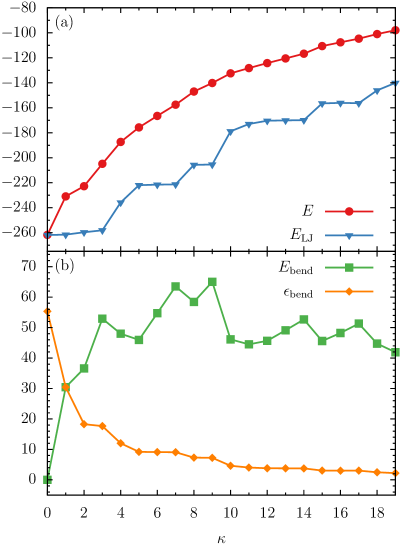
Figure 1: (a) Total energy $E$ and Lennard-Jones contribution $E_{\mathrm{LJ}}$ of ground-state conformations. (b) Total bending energy $E_{\mathrm{bend}}$ and renormalized bending contributions $\epsilon_{\mathrm{bend}}=E_{\mathrm{bend}}/\kappa$ for the entire array of $\kappa$ parameter values simulated.

In this section, we perform a detailed analysis of the different energy contributions governing ground-state conformations of semiflexible polymers and discuss geometric properties based on the gyration tensor. Eventually, we introduce monomer-distance and monomer-contact maps to investigate internal structural patterns.

III.0.1 Energy Contributions

Putative ground-state conformations and their energies obtained from simulations for different choices of the bending stiffness $\kappa$ are listed in Tab. 1. By increasing the bending stiffness $\kappa$, the semiflexible polymer folds into different classes of structures: compact globules ($\kappa<5$), rod-like bundles ($5\leq\kappa\leq 9$), as well as toroids ($\kappa>9$).

In order to better understand the crossover from one structure type to another, we first investigate the separate contributions from LJ and bending potentials to the total ground-state energies. Since bond lengths are at almost optimal distances ($\approx r_{0}$), the bonded potential $V_{\mathrm{FENE}}$ can be ignored in the following analysis. The main competition is between

$$E_{\mathrm{LJ}}=\sum_{i>j}\left(V_{\mathrm{LJ}}(r_{i,j})-V_{\mathrm{shift}}\right),$$ (10)

including contributions from bonded monomers, and the bending energy

$$E_{\mathrm{bend}}=\sum_{l}V_{\mathrm{bend}}(\theta_{l}).$$ (11)

We also introduce the renormalized contribution from the bending potential

$$\epsilon_{\mathrm{bend}}=E_{\mathrm{bend}}/\kappa$$ (12)

for studying the relative impact of bending on these conformations.

The energies $E$, $E_{\mathrm{LJ}}$, bending energy $E_{\mathrm{bend}}$, and renormalized bending quantity $\epsilon_{\mathrm{bend}}$ are plotted for all ground-state conformations in Fig. 1. Not surprisingly, the total energy $E$ increases as the bending stiffness $\kappa$ increases. Similarly, $E_{\mathrm{LJ}}$ also increases with increased bending stiffness $\kappa$, but rather step-wise. Combining these trends with the corresponding structures, it can be concluded that each major global change in ground-state conformations with increased bending stiffness leads to the reduced attraction between monomers (increase in $E_{\mathrm{LJ}}$). Whereas the bending energy $E_{\mathrm{bend}}$ does not exhibit a specific trend, the renormalized bending energy $\epsilon_{\mathrm{bend}}$ decreases step-wise as well for increased bending stiffness $\kappa$, as shown in Fig. 1(b). It is more interesting, though, to see there are clear alterations of $E_{\mathrm{LJ}}$ and $\epsilon_{\mathrm{bend}}$ within the same structure type (compact globules, rod-like bundles, or toroids).

In certain $\kappa$ intervals (e.g., $3<\kappa<5$ and $9<\kappa<10$), a rapid increase in $E_{\mathrm{LJ}}$ correlates with a decrease in $\epsilon_{\mathrm{bend}}$, which seems to be counter-intuitive. However, these are the regions, in which the structural type of the ground state changes significantly. This means a loss of energetically favorable contacts between monomers is not primarily caused by a higher bending penalty, but rather the global rearrangement of monomers.

For $\kappa=0,1$ and $2$, the overall attraction $E_{\mathrm{LJ}}$ does not change much, in contrast to $\epsilon_{\mathrm{bend}}$, suggesting that the polymer chain is able to accommodate the bending penalty without affecting energetically favorable monomer-monomer contacts.

Even though the energetic analysis provides more information about the competition between different energetic terms, conclusions about the structural behavior are still qualitative. Therefore, a more detailed structural analysis is performed in the following.

III.0.2 Gyration Tensor Analysis

In order to provide a quantitative description of the structural features, we calculated the gyration tensor $S$ for the ground-state conformations with components

$$S_{\alpha,\beta}=\frac{1}{N}\sum_{i=1}^{N}\left(r_{\alpha}^{(i)}-r_{\alpha}^{\mathrm{CM}}\right)\left(r_{\beta}^{(i)}-r_{\beta}^{\mathrm{CM}}\right),$$ (13)

where $\alpha,\beta\in\left\{x,y,z\right\}$ and $\bm{r}^{\mathrm{CM}}=\frac{1}{N}\sum_{j=1}^{N}\bm{r}_{j}$ is the center of mass of the polymer. After diagonalization, $S$ can be written as

$$S_{\mathrm{D}}=\begin{pmatrix}\lambda^{2}_{x}&0&0\\ 0&\lambda^{2}_{y}&0\\ 0&0&\lambda^{2}_{z}\end{pmatrix},$$ (14)

where the eigenvalues are principal moments and ordered as $\lambda_{x}^{2}\leq\lambda_{y}^{2}\leq\lambda_{z}^{2}$. These moments describe the effective extension of the polymer chain in the principal axial directions. Thus, different invariant shape parameters can be derived from combinations of these moments. Most commonly used for polymers, the square radius of gyration $R^{2}_{\mathrm{gyr}}$ is obtained from the summation of the eigenvalues:

$$R^{2}_{\mathrm{gyr}}=\lambda^{2}_{x}+\lambda^{2}_{y}+\lambda^{2}_{z}.$$ (15)

The radius of gyration describes the overall effective size of a polymer conformation. In addition, another invariant shape parameter we employed is the relative shape anisotropy $A$, which is defined as

$$A=\frac{3}{2}\frac{\lambda^{4}_{x}+\lambda^{4}_{y}+\lambda^{4}_{z}}{\left(\lambda^{2}_{x}+\lambda^{2}_{y}+\lambda^{2}_{z}\right)^{2}}-\frac{1}{2}.$$ (16)

It is a normalized parameter, the value of which is limited to the interval $A\in[0,1]$, where $A=0$ is associated with spherically symmetric polymer chains ($\lambda_{x}=\lambda_{y}=\lambda_{z}$), and $A=1$ is the limit for the perfectly linear straight chain ($\lambda_{x}=\lambda_{y}=0,\lambda_{z}>0$). Other than these two limits, $A=1/4$ refers to perfectly planar conformations ($\lambda_{x}=0,0<\lambda_{y}=\lambda_{z}$). Square principal components $\lambda_{x}^{2},\lambda_{y}^{2},\lambda_{z}^{2}$, square radius of gyration $R^{2}_{\mathrm{gyr}}$, and the relative shape anisotropy $A$ of ground-state conformations are plotted in Fig. 2 as functions of $\kappa$.

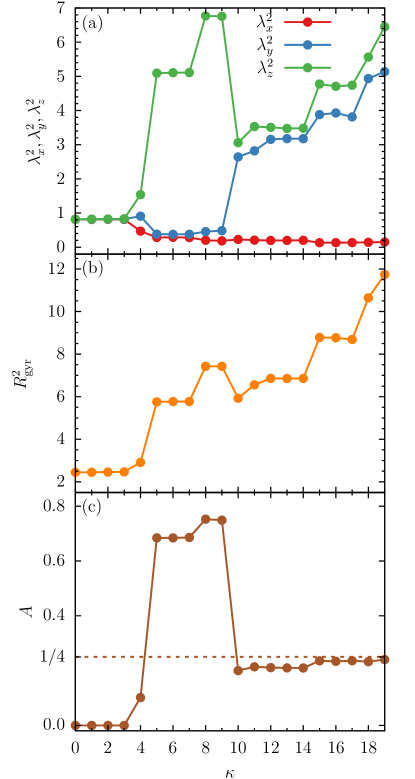
Figure 2: (a) Square principal moments $\lambda_{x}^{2},\lambda_{y}^{2},\lambda_{z}^{2}$ from the diagonalized gyration tensor $S$, (b) square radius of gyration $R^{2}_{\mathrm{gyr}}$, (c) and relative shape anisotropy $A$ for ground-state conformations on a large array of $\kappa$ values.

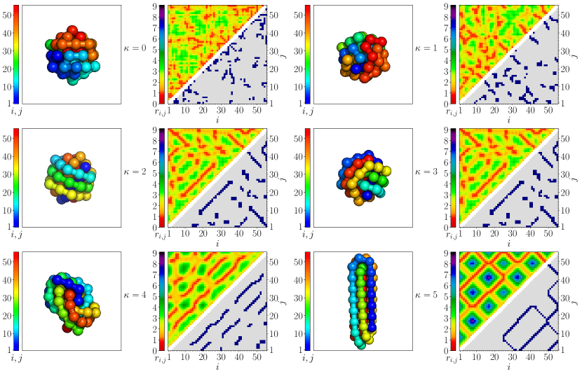
Figure 3: Representations of ground-state conformations (left panel) and their contact maps (right) for $\kappa\leq 5$. The upper triangle contains the monomer distance map, where the distance $r_{i,j}$ of monomers $i$ and $j$ is colored. The contact map is shown in the lower triangle. Monomers $i$ and $j$ are in contact if $r_{i,j}<1.2$.

Starting with $\kappa=0,1,2$ and $3$, the three principal moments of the corresponding lowest-energy conformations are small and nearly equal. These are the most compact conformations we found (see Tab. 1). For these structures, $A<10^{-3}$. Furthermore, for $\kappa<4$, lowest-energy conformations of semiflexible polymers possess an icosahedral-like arrangement of monomers, similar to that of the purely flexible chain ($\kappa=0$).

For $\kappa=4$, the increased bending stiffness already forces conformations to stretch out noticeably. This is reflected by the imbalance of the principal moments. Consequently, $A$ is nonzero and the overall size of the conformations becomes larger as $R^{2}_{\mathrm{gyr}}$ suggests.

If the bending stiffness is increased to $\kappa=5,6$ and $7$, rod-like structures with $7$ bundles are formed to minimize the total energy. One principal moment increases dramatically while the other two moments decrease. As a result, $R^{2}_{\mathrm{gyr}}$ reaches a higher level, but remains almost constant in this $\kappa$ range. The relative shape anisotropy climbs to $A\approx 0.69$, indicating that the shape straightens out further.

The number of bundles reduces to six for $\kappa=8$ and $9$, resulting in longer rod-like structures. Both $R^{2}_{\mathrm{gyr}}$ and $A$ increase further, the change of which is not visually obvious in Tab. 1, though.

With the bending energy even more dominant for $10\leq\kappa\leq 14$, the appearance of conformations changes significantly. Toroidal structures with up to $4$ windings are energetically more favored than rod-like bundles. Instead of forming a few sharp turns to accommodate the bending penalty as in the bundled conformations, the polymer chain now takes on a rather dense toroidal shape. Successive bending angles are comparatively small. In this case, the two largest principal moments converge to an intermediate value. As a consequence of the more compact structures, $R^{2}_{\mathrm{gyr}}$ decreases with increased bending stiffness. The asphericity $A$ drops below the characteristic limit $1/4$, reflecting the planar symmetry of the toroidal structures.

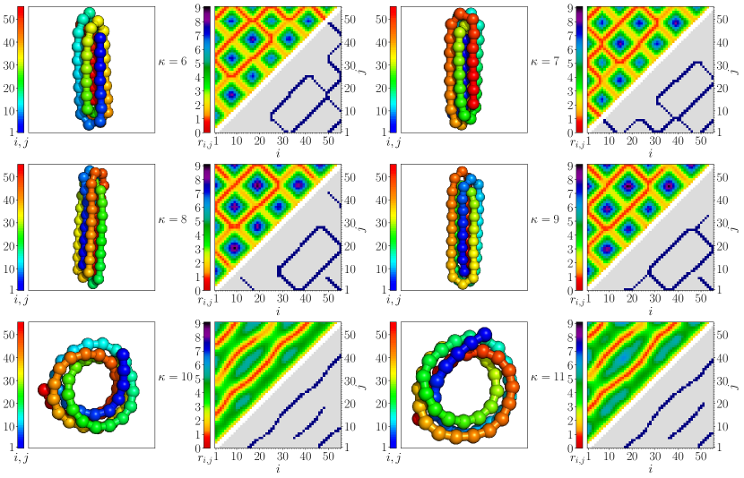
Figure 4: Same as Fig. 3, but for $6\leq\kappa\leq 11$.

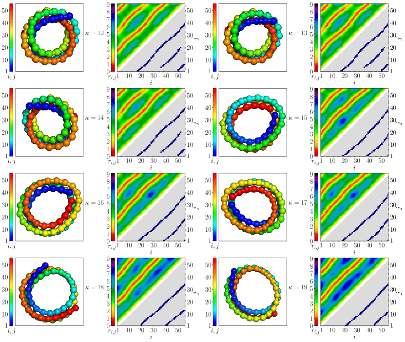
Figure 5: Same as Fig. 3, but for $\kappa\geq 11$.

It becomes more difficult for the polymer in the ground state to maintain the same small bending angles for increased bending stiffness values $\kappa=15,16$ and $17$. As a result, whereas the smaller bending angles still cause similar toroidal structures as in the previously discussed case, the radius of the toroids increases and fewer windings are present. Therefore, two main principal moments increase, as well as $R^{2}_{\mathrm{gyr}}$. Meanwhile, the relative shape anisotropy $A$ approaches $1/4$. Fewer windings reduce the overall thickness in the normal direction of the toroidal conformations. As can be seen from the conformations in Tab. 1, these structures are stabilized by the attraction of close end monomers.

However, for $\kappa>17$, the attraction of two end monomers is not sufficient to sustain the structure. Thus, expanding the toroid becomes an advantageous option to offset strong bending penalties. The toroidal structure is stretched out, which is clearly seen in Tab. 1 for $\kappa=18$ and $19$. The radius of the toroid keeps getting larger, so does $R^{2}_{\mathrm{gyr}}$. We find that $A$ keeps converging to the planar symmetry limit of $1/4$.

It is expected that increasing the bending stiffness further ultimately leads to a loop-like ground state and eventually to an extended chain, in which case no energetic contacts that could maintain the internal structural symmetries are present anymore.

III.0.3 Contact Map Analysis

Even though the previous gyration tensor analysis yields a reasonable quantitative description of the overall structural properties of the ground-state conformations, it does not provide insight into internal structures. Therefore, we now perform a more detailed analysis by means of monomer distance maps and contact maps.

To find the relative monomer positions, we measured the monomer distance $r_{i,j}$ between monomers $i$ and $j$ for all monomer pairs. Furthermore, we consider nonbonded monomer pairs with distances $r_{i,j}<1.2$ to be in contact. The limit, which is close to the minimum distance $r_{0}$ of the Lennard-Jones potential, allows to distinguish unique contact features of conformations while avoiding counting nonnearest-neighbor contacts. In the figures, we colored the monomers from one end to the other to visualize the chain orientation.

The combined results for $\kappa\leq 5$ are shown in Fig. 3. For $\kappa=0$ (flexible polymer), the structure is icosahedral, and the maps do not exhibit particularly remarkable structural features. Without the energetic penalty from bending, maximizing the number of nearest neighbors is the optimal way to gain energetic benefit. For $\kappa=1$, the introduced small bond angle restraint already starts affecting the monomer positions. In the contact map, short anti-diagonal streaks start appearing, which indicate the existence of a U-turn like segment with two strands in contact. Interestingly, we find similar conformations for $\kappa=2$ and $\kappa=3$, as confirmed by similar distance and contact maps. There are fewer, but longer anti-diagonal strands, located in the interior of the compact structure. The formation of new streaks parallel to the diagonal is associated with the helical wrapping of monomers, which is visible in the colored representations. As for $\kappa=4$, the ground-state conformation is the compromise of two tendencies. The bending stiffness neither is weak, as for $\kappa=3$ the semiflexible polymer is still able to maintain a spherical compact structure with more turns, nor is it particularly strong as for $\kappa=5$, where the polymer forms a rod-like bundle structure. Therefore, the lowest-energy conformations shown in Fig. 3 contain only helical turns trying to minimize the size, as indicated by several diagonal streaks in the contact map. For $\kappa=5$, the polymer mediates the bending penalty by allowing only a few sharp turns between the rods. For the $7$-bundle structure, the randomness completely disappears in both distance and contact maps. The blue square areas in the distance map mark the separation of monomer groups belonging to the two ends of a bundle. Furthermore, the diagonal streaks indicate the contact of two parallel bundles while the turns of the chain form anti-diagonal streaks. It is also worth mentioning that in this case the two end monomers are located on opposite sides.

The results for $6\leq\kappa\leq 11$ are shown in Fig. 4. Similar to $\kappa=5$, the polymer still forms a $7$-bundle rod-like structure for $\kappa=6$ and $\kappa=7$. The anti-diagonal symmetry in maps for $\kappa=6$ and $\kappa=7$ is only a consequence of opposite indexing of monomers. For $\kappa=8$ and $\kappa=9$, the increased bending stiffness leads to a decrease in the number of sharp turns from $7$ to $6$, where the two end monomers are now located on the same side. The relative positions of monomers are almost identical for $\kappa=8$ and $\kappa=9$ as seen in their distance maps. However, the difference in contact maps is caused by the way the straight rods following the sharp turns are aligned. For $\kappa=8$, four monomers (the orange turn in the colored presentation in Fig. 4 for $\kappa=8$) form the sharp turn. This allows the rods to align closer compared to the $\kappa=9$ case, where only $3$ monomers are located in the turn that holds two parallel rods (blue shades). For $\kappa=10,11$, the optimal way to pack monomers is by toroidal wrapping. Thus, the contact maps exhibit only three diagonal streaks.

Results for $\kappa\geq 11$ are shown in Fig. 5. Contact maps for $\kappa=12,13$ and $14$ still feature three diagonal streaks. However, for $\kappa=15,16$, and $17$, the increased bending stiffness causes a larger radius of the toroidal structure and the two end monomers are stabilized by Lennard-Jones attraction. Thus, the number of parallel diagonals reduces to two and the attraction of two end monomers is marked in the corners of the maps. Finally, for polymers with even larger bending stiffness, i.e., $\kappa=18$ and $\kappa=19$, the contact between the two end monomers breaks and the whole structure stretches out even more. As a result, the distance map for $\kappa=19$ contains extended sections of increased monomer distances. At the same time, the contact map still shows two streaks slightly shifted to the right, indicating a reduction in the number of contacts.

IV Summary

In this study, we have examined the effect of bending stiffness on ground-state conformations of semiflexible polymers by using a coarse-grained model. In order to obtain estimates of the ground-state energies, we employed an extended version of parallel tempering Monte Carlo and verified our results by means of global optimization algorithms. We find that the semiflexible polymer folds into compact globules for relatively small bending stiffness, rod-like bundles for intermediate bending strengths, as well as toroids for sufficiently large bending restraints. Eventually, we performed energetic and structural analyses to study the impact of the bending stiffness on the formation of ground-state structures.

We decomposed the energy contributions to gain more insight into the competition between attractive van der Waals forces and the bending restraint. The total energy of ground-state conformations increases smoothly with increased bending stiffness, but not the attraction and bending potentials. Interestingly, renormalizing the bending energy reveals that local bending effects of ground-state conformations actually reduce for increased bending stiffness.

The structural analysis by means of gyration tensor and invariant shape parameters provided a general picture regarding the size and shape changes of conformations under different bending restraints. In a further step, studying distance maps and contact maps exposed details of internal structure ordering and helped distinguish conformations, especially for small values of the bending stiffness, where the gyration tensor analysis has been inconclusive. Contact map analysis also caught slight differences, where different structure types are almost degenerate.

In conclusion, the bending stiffness significantly influences the formation of low-energy structures for semiflexible polymers. Varying the bending stiffness parameter in our model results in shapes like compact globules, rod-like bundles, and toroids with abundant internal arrangements. Semiflexible polymer structures remain stable within a certain range of bending strengths, which makes them obvious candidates for functional macromolecules. Monomer-monomer attraction provides stability and bending stiffness adaptability to allow semiflexible polymers to form distinct structures under diverse physiological conditions ab23 .

Data Availability Statement

The data that support the findings of this study are available from the corresponding author upon reasonable request.

References

- (1) L. M. C. Sagis, C. Veerman, and E. van der Linden, Langmuir 20, 924 (2004).
- (2) L. David, A. Thakkar, R. Mercado, and O. Engkvist, J. Cheminformatics 12, 56 (2020).
- (3) G. Macetti and A. Genoni, J. Phys. Chem. A 123, 9420 (2019).
- (4) M. Vendruscolo and C. M. Dobson, Current Biology 21, R68 (2011).
- (5) M. Bachmann, Thermodynamics and Statistical Mechanics of Macromolecular Systems (Cambridge University Press, Cambridge, 2014).
- (6) D. T. Seaton, S. Schnabel, D. P. Landau, and M. Bachmann, Phys. Rev. Lett. 110, 028103 (2013).
- (7) J. Zierenberg and W. Janke, Europhys. Lett. 109, 28002 (2015).
- (8) J. Wu, C. Cheng, G. Liu, P. Zhang, and T. Chen, J. Chem. Phys. 148, 184901 (2018).
- (9) S. Majumder, M. Marenz, S. Paul, and W. Janke, Macromolecules 54, 5321 (2021).
- (10) C. C. Walker, T. L. Fobe, and M. R. Shirts, Macromolecules 55, 8419 (2022).
- (11) H. G. Garcia, P. Grayson, L. Han, M. Inamdar, J. Kondev, P. C. Nelson, R. Phillips, J. Widom, and P. A. Wiggins, Biopolymers 85, 115 (2007).
- (12) S. Li, G. Erdemci-Tandogan, P. van der Schoot, and R. Zandi, J. Phys. : Condens. Matter. 30, 044002 (2018).
- (13) J. P. Richard, J. Am. Chem. Soc. 141, 3320 (2019).
- (14) O. Kratky and G. Porod, J. Colloid Sci. 4, 35 (1949).
- (15) M. Hegner, S. B. Smith, and C. Bustamante, Proc. Nat. Acad. Soc. 96, 10109 (1999).
- (16) I. M. Kulić and H. Schiessel, Phys. Rev. Lett. 92, 228101 (2004).
- (17) D. G. Angelescu and P. Linse, Phys. Rev. E 75, 051905 (2007).
- (18) Q. Cao and M. Bachmann, Phys. Rev. E 90, 060601(R) (2014).
- (19) D. Aierken and M. Bachmann, Polymers 12, 3013 (2020).
- (20) R. H. Swendsen and J.-S. Wang, Phys. Rev. Lett. 57, 2607 (1986).
- (21) C. J. Geyer, Computing Science and Statistics: Proceedings of the 23rd Symposium on the Interface, edited by E. M. Keramidas (Interface Foundation, Fairfax Station VA, 1991), 156.
- (22) K. Hukushima and K. Nemoto, J. Phys. Soc. Jpn. 65, 1604 (1996).
- (23) K. Hukushima, H. Takayama, and K. Nemoto, Int. J. Mod. Phys. C 07, 337 (1996).
- (24) D. J. Earl and M. W. Deem, Phys. Chem. Chem. Phys. 7, 3910 (2005).
- (25) S. Schnabel, W. Janke, and M. Bachmann, J. Comput. Phys. 230, 4454 (2011).
- (26) K. S. Austin, M. Marenz, and W. Janke, Comput. Phys. Commun. 224, 222 (2018).
- (27) A. Milchev, A. Bhattacharya, and K. Binder, Macromolecules 34, 1881 (2001).
- (28) K. Kremer and G. S. Grest, J. Chem. Phys. 92, 5057 (1990).
- (29) R. B. Bird, C. F. Curtiss, R. C. Armstrong, and O. Hassager, Dynamics of Polymeric Liquids, 2nd edition (Wiley, New York, 1987).
- (30) K. Qi and M. Bachmann, J. Chem. Phys. 141, 074101 (2014).
- (31) F. Wang and D. P. Landau, Phys. Rev. Lett. 86, 2050 (2001).
- (32) S. Schnabel and W. Janke, Comput. Phys. Commun. 267, 108071 (2021).
- (33) S. Kirkpatrick, C. D. Gelatt, and M. P. Vecchi, Science 220, 671 (1983).
- (34) U. H. E. Hansmann and L. T. Wille, Phys. Rev. Lett. 88, 068105 (2002).
- (35) D. Aierken and M. Bachmann, Phys. Rev. E 107, L032501 (2023).