Improving Accelerated Federated Learning with Compression and Importance Sampling

Abstract

Federated Learning is a collaborative training framework that leverages heterogeneous data distributed across a vast number of clients. Since it is practically infeasible to request and process all clients during the aggregation step, partial participation must be supported. In this setting, the communication between the server and clients poses a major bottleneck. To reduce communication loads, there are two main approaches: compression and local steps. Recent work by Mishchenko et al. (2022) introduced the new ProxSkip method, which achieves an accelerated rate using the local steps technique. Follow-up works successfully combined local steps acceleration with partial participation (Grudzień et al., 2023; Condat et al., 2023) and gradient compression (Condat et al., 2022). In this paper, we finally present a complete method for Federated Learning that incorporates all necessary ingredients: Local Training, Compression, and Partial Participation. We obtain state-of-the-art convergence guarantees in the considered setting. Moreover, we analyze the general sampling framework for partial participation and derive an importance sampling scheme, which leads to even better performance. We experimentally demonstrate the advantages of the proposed method in practice.

1 Introduction

Federated Learning (FL) (Konečný et al., 2016; McMahan and Ramage, 2017) is a distributed machine learning paradigm that allows multiple devices or clients to collaboratively train a shared model without transferring their raw data to a central server. In traditional machine learning, data is typically gathered and stored in a central location for training a model. However, in Federated Learning, each client trains a local model using its own data and shares only the updated model parameters with a central server or aggregator. The server then aggregates the updates from all clients to create a new global model, which is then sent back to each client to repeat the process (McMahan et al., 2016).

This approach has gained significant attention due to its ability to address the challenges of training machine learning models on decentralized and sensitive data McMahan et al. (2017). Federated Learning enables clients to preserve their privacy and security by keeping their data local and not sharing it with the central server. This approach also reduces the need for large-scale data transfers, thereby minimizing communication costs and latency (Li et al., 2020a).

Federated Learning poses several challenges such as data heterogeneity, communication constraints, and ensuring the privacy and security of the data (Kairouz et al., 2021). Researchers in this field have developed novel optimization algorithms to address these challenges and to enable efficient aggregation of the model updates from multiple clients (Wang et al., 2021b). Federated Learning has been successfully applied to various applications, including healthcare (Vepakomma et al., 2018), finance (Long et al., 2020), and Internet of Things (IoT) devices (Khan et al., 2021).

This work considers the standard formulation of Federated Learning as a finite sum minimization problem:

$$\min_{x\in\mathbb{R}^{d}}\left[f(x)\coloneqq\frac{1}{M}\sum_{m=1}^{M}f_{m}(x)\right]$$ (1)

where $M$ is the number of clients/devices. Each function $f_{m}(x)=\mathbb{E}_{\xi\sim\mathcal{D}_{m}}\left[l(x,\xi)\right]$ represents the average loss, calculated via the loss function $l$, of the model parameterized by $x\in\mathbb{R}^{d}$ over the training data $\mathcal{D}_{m}$ stored by client $m\in\left[M\right]\coloneqq\left\{1,\ldots,M\right\}.$

1.1 Federated Averaging

The method known as Federated Averaging (FedAvg), proposed by McMahan et al. (2017), is a widely used technique that specifically addresses the challenges of practical federated environments while solving problem 1. FedAvg is based on Gradient Descent (GD), but applies four modifications: Client Sampling (CS), Data Sampling (DS), Local Training (LT), Communication Compression (CC).

The FedAvg training process occurs over several communication rounds. At the start of each round $t$, a subset or cohort $S^{t}\subset[M]$ of clients with a size of $C^{t}=|S^{t}|$ is selected to participate in that round’s training. The aggregating server then sends the current model version, $x^{t}$, to all clients $m\in S^{t}$. Each client $m\in S^{t}$ performs $K$ iterations of SGD on its local loss function, $f_{m}$, using minibatches $\mathcal{B}_{m}^{k,t}\subseteq\mathcal{D}_{m}\text{ of size }b_{m}=\left|\mathcal{B}_{m}^{k,t}\right|\text{ for }k=0,\ldots,K-1$ initialized with $x^{t}$. Afterward, all participating clients compress their updated models and send these compressed updates to the server to aggregate into a new model version, $x^{t+1}$. The entire process is then repeated. This generalized scheme is described in Grudzień et al. (2023).

Each of the four FedAvg modifications, Client Sampling (CS), Data Sampling (DS), Local Training (LT), and Communication Compression can be independently turned on or off, or used in various combinations. For instance, if $C^{t}=M$ for all rounds, then all clients take part in every round, resulting in the deactivation of CS. Similarly, when $b_{m}=|D_{m}|$ for each client $m\in[M]$, every client employs all their data to compute the local gradient estimator needed for SGD, which leads to the deactivation of DS. Additionally, when $K$ is set to $1$, each participating client performs only one SGD step, causing LT to be turned off. Lastly, If the compression operator is set to the identity, then each client transmits complete updates, resulting in compression being turned off. If all four modifications are disabled, FedAvg becomes equivalent to vanilla gradient descent (GD).

1.2 Data Sampling

The seminal works discussed earlier illustrate the practical benefits of the novel approach, i.e., FedAvg method, but they lack theoretical analysis and associated guarantees. Given that FedAvg comprises four distinct components, it is expedient to analyze these techniques in isolation to achieve a deeper comprehension of each of them.

Due to the close association of unbiased data sampling techniques with the stochastic approximation literature dating back to the works of Robbins and Monro (1951); Nemirovsky and Yudin (1983); Nemirovski et al. (2009); Bottou et al. (2018), it is not unexpected that CS is comparatively well comprehended. For instance, Gower et al. (2019) have scrutinized variations of SGD that back almost any unbiased CS mechanism in the smooth strongly convex area, while Khaled and Richtárik (2020) have analyzed those in the smooth nonconvex region. Furthermore, Tyurin et al. (2022a) have proposed and studied oracle-optimal versions of SGD that support almost any unbiased CS and DS mechanisms in the smooth nonconvex region, drawing upon the previous works of Li et al. (2021), Fang et al. (2018), and Nguyen et al. (2017a, b). The CS with variance reduction techniques is widely analyzed by Gorbunov et al. (2020).

1.3 Client Sampling

As distributed learning gained popularity, researchers began to examine Client Sampling strategies for improving communication efficiency (Wu and Wang, 2022) and ensuring robustness and security during aggregation (So et al., 2021). Empirical studies of Client Sampling strategies can be found in the literature, such as Fraboni et al. (2021); Charles et al. (2021); Huang et al. (2022). Optimal Client Sampling strategies under various conditions have been theoretically analyzed in works such as Wang et al. (2022) and Chen et al. (2022). The cyclic patterns of client participation are studied in Malinovsky et al. (2023); Cho et al. (2023). While Client Sampling shares similarities with data sampling, it also has distinct characteristics that need to be taken into account.

1.4 Communication Compression

Communication Compression is a valuable component in distributed optimization, as it allows each client to transmit a compressed or quantized version of its update, $\Delta^{t}_{m}$, instead of the entire update vector. This can lead to significant bandwidth savings by reducing the number of bits transmitted over the network. Various operators have been proposed for compressing update vectors, such as stochastic quantization (Alistarh et al., 2017), random sparsification (Wangni et al., 2017; Stich et al., 2018), and alternative methods (Tang et al., 2019).

The utilization of unbiased compressors can decrease the amount of bits that clients transmit per round. However, it can also cause an increase in the variance of the stochastic gradients, which leads to a slower overall convergence (Khirirat et al., 2018; Stich, 2020). To address this issue, Mishchenko et al. (2019) proposed DIANA, an algorithm that uses control iterates to diminish the variance resulting from gradient compression with unbiased compression operators. This approach guarantees fast convergence. DIANA has been examined and extended in various scenarios (Horváth et al., 2019; Safaryan et al., 2021; Wang et al., 2021a; Kovalev et al., 2021; Li et al., 2020d) and is a valuable tool for utilizing gradient compression.

The article presents the application of compression techniques in Federated Learning, as discussed in Basu et al. (2019); Reisizadeh et al. (2020); Haddadpour et al. (2021). The mechanism of compressing iterates is studied in Khaled and Richtárik (2019); Chraibi et al. (2019). Additionally, Malinovsky and Richtárik (2022) and Sadiev et al. (2022b) investigate the application of compression with random reshuffling in Federated Learning.

1.5 Five Generations of Local Training

Local Training (LT) is a crucial aspect of Federated Learning (FL) models, where each participating client performs multiple local optimization steps before synchronization of parameters. In the smooth strongly convex regime, we will provide a concise overview of the theoretical advancements made in understanding LT. Malinovsky et al. (2022b) categorized LT methods into five generations - heuristic, homogeneous, sublinear, linear, and accelerated - each progressively enhancing the previous one in significant ways.

1st (heuristic) generation of LT methods. Although the ideas behind LT were previously utilized in various machine learning fields Povey et al. (2015); Moritz et al. (2016), it gained significant attention as a communication acceleration technique following seminal paper introducing the FedAvg algorithm (McMahan et al., 2017). However, their work, along with previous research, lacked any theoretical justification. As a result, LT-based heuristics dominated the field’s initial development until the FedAvg paper and lacked any theoretical guarantees.

2nd (homogeneous) generation of LT methods )The second generation of LT methods offers guarantees, but their analysis relies on various data homogeneity assumptions. These assumptions include bounded gradients, which require $\left\|\nabla f_{m}(x)\right\|\leq c$ for all $m\in[M]$ and $x\in\mathbb{R}^{d}$ (Li et al., 2020c), or bounded gradient dissimilarity, i.e., requiring $\frac{1}{M}\sum_{m=1}^{M}\left\|\nabla f_{m}(x)\right\|^{2}\leq c\|\nabla f(x)\|^{2}\text{ for all }x\in\mathbb{R}^{d}$ (Haddadpour and Mahdavi, 2019). The reasoning behind such assumptions is that in the extreme case when all local functions are identical, running GD independently and in parallel on all clients without any communication or averaging would make GD communication-efficient. Based on this, as we increase heterogeneity, taking multiple local steps should still be beneficial as long as the number of steps is limited. However, using bounded dissimilarity assumptions is highly problematic as they are not met even in some of the simplest function classes, such as strongly convex quadratics (Khaled et al., 2019a, b). Furthermore, due to the highly heterogeneous and non-i.i.d nature of real-world federated learning datasets, relying on strong assumptions like data/gradient homogeneity for analyzing LT methods is both mathematically dubious and practically insignificant. Several authors have analyzed various LT methods under such assumptions and obtained rates (Yu et al., 2019; Li et al., 2019, 2020b)

3rd (sublinear) generation of LT methods. The third generation LT theory successfully eliminated the need for data homogeneity assumptions, as demonstrated by Khaled et al. (2019a, b). However, subsequent studies by Woodworth et al. (2020b) and Glasgow et al. (2022) showed that LocalGD with DS (LocalSGD) has communication complexity that is no better than minibatch SGD in the heterogeneous data setting. Furthermore, Malinovsky et al. (2020) analyzed LT methods for general fixed point problems and Koloskova et al. (2020) studied decentralized accepts of Local Training. While removing the need for data homogeneity assumptions was a significant advancement, the results were rather pessimistic, indicating that LT-enhanced GD, or LocalGD, has a sublinear convergence rate, which is inferior to vanilla GD’s linear convergence rate (Woodworth et al., 2020a). The effect of server-side stepsizes is analyzed in Malinovsky et al. (2022a); Charles and Konečnỳ (2020)

4th (linear) generation of LT methods. The focus of the fourth generation of LT methods was to develop linearly converging versions of LT algorithms by addressing the problem of client drift, which was identified as the reason behind the previous generation’s subpar performance compared to GD. The first method to successfully mitigate client drift and achieve a linear convergence rate was Scaffold, as proposed by Karimireddy et al. (2020). Other approaches to achieve the same effect were later introduced by Gorbunov et al. (2021) and Mitra et al. (2021). While obtaining a linear rate under standard assumptions was a significant achievement, these methods still have a slightly higher communication complexity than vanilla GD and at best equal to that of GD.

5th (accelerated) generation of LT methods. Mishchenko et al. (2022) have recently introduced the ProxSkip method, which represents a new and simple approach to Local Training that results in provable communication acceleration in the smooth strongly convex regime, even when dealing with heterogeneous data. Specifically, in cases where each $f_{m}$ is $L$-smooth and $\mu$-strongly convex, ProxSkip can solve 1 in $\mathcal{O}(\sqrt{L/\mu}\log 1/\varepsilon)$ communication rounds, a significant improvement over the $\mathcal{O}(L/\mu\log 1/\varepsilon)$ complexity of GD. This accelerated communication complexity has been shown to be optimal by Scaman et al. (2019). Mishchenko et al. (2022) have also introduced several extensions to ProxSkip, including a flexible data sampling framework and decentralized version. As a result of these developments, other new methods that can achieve communication acceleration using Local Training are proposed.

The initial sequel article by Malinovsky et al. (2022b) presents a broad variance reduction structure for the ProxSkip approach. In addition, Condat and Richtárik (2022) applies the ProxSkip methodology to complex splitting schemes that involve the sum of three operators in a forward-backward setting. Besides,Sadiev et al. (2022a) and Maranjyan et al. (2022) improve the computational complexity of the ProxSkip method while maintaining its accelerated communication acceleration.Condat et al. (2023) introduces accelerated Local Training methods that allow Client Sampling based on the ProxSkip method, and Grudzień et al. (2023) provide an accelerated method with Client Sampling based on RandProx method with primal and dual updates. However, these methods are limited as they only work with a uniform distribution of clients. CompressedScaffnew (Condat et al., 2022) is the first LT method to achieve accelerated communication complexity while utilizing compression of updates. However, it works only with permutation-based compressors (Szlendak et al., 2022), and it is not compatible with a broad range of unbiased compressors. Permutation-based compressors demand synchronization of compression patterns during the aggregation stage, which is not feasible for Federated Learning settings due to privacy aspects.

2 Contributions

Our work is based on the observation that none of the 5th generation Local Training (LT) methods currently support both Client Sampling (CS) and Communication Compression (CC). This raises the question of whether it is possible to design a method that can benefit from communication acceleration via LT while also supporting CS and utilizing Communication Compression techniques.

At this point, we are prepared to summarize the crucial observations and contributions made in our work.

• To the best of our knowledge, we provide the first LT method that successfully combines communication acceleration through local steps, Client Sampling techniques, and Communication Compression for a wide range of unbiased compressors. Our proposed algorithm for distributed optimization and federated learning is the first of its kind to utilize both strategies in combination, resulting in a doubly accelerated rate. Our method based on method 5GCS (Grudzień et al., 2023) benefits from the two acceleration mechanisms provided by Local Training and compression in the Client Sampling regime, exhibiting improved dependency on the condition number of the functions and the dimension of the model, respectively.

• In this paper, we investigate a comprehensive Client Sampling framework based on the work of  Tyurin et al. (2022b), which we then apply to the 5GCS method proposed by Grudzień et al. (2023). This approach enables us to analyze a wide range of Client Sampling techniques, including both sampling with and without replacement and it recovers previous results for uniform distribution. The framework also allows us to determine optimal probabilities, which results in improved communication.

3 Preliminaries

3.1 Method’s description

This section provides a description of the proposed methods in this paper. Specifically, we consider two algorithms (Algorithm 1 and Algorithm 2), both of which share the same core idea. At the beginning of the training process, we initialize several parameters, including the starting point $x^{0}$, the dual (control) iterates $u^{0}_{1},\ldots,u^{0}_{M}$, the primal (server-side) stepsize, and $M$ dual (local) stepsizes. Additionally, we choose a sampling scheme $\mathbf{S}$ for Algorithm 1 or a type of compressor $\mathcal{Q}$ for Algorithm 2. Once all parameters are set, we commence the iteration cycle.

At the start of each communication round, we sample a cohort (subset) of clients according to a particular scheme. The server then computes the intermediate model $\hat{x}^{t}$ and sends this point to each client in the cohort. Once each client receives the model $\hat{x}^{t}$, the worker uses it as a starting point for solving the local sub-problem defined in Equation 4. After approximately solving the local sub-problem, each client computes the gradient of the local function at the approximate solution $\nabla F_{m}(y^{K,t}_{m})$ and, based on this information, each client forms and sends an update to the server, either with or without compression. The server then aggregates the received information from workers and updates the global model $x^{t+1}$ and additional variables if necessary. This process repeats until convergence.

3.2 Assumptions

We begin by adopting the standard assumption in convex optimization (Nesterov, 2004).

Assumption 1.

The functions $f_{m}$ are $L_{m}$-smooth and $\mu_{m}$-strongly convex for all $m\in\left\{1,...,M\right\}.$

All of our theoretical results will rely on this standard assumption in convex optimization. To recap, a continuously differentiable function $\phi:\mathbb{R}^{d}\rightarrow\mathbb{R}$ is $L$-smooth if $\phi(x)-\phi(y)-\langle\nabla\phi(y),x-y\rangle\leq\frac{L}{2}\|x-y\|^{2}$ for all $x,y\in\mathbb{R}^{d}$, and $\mu$-strongly convex if $\phi(x)-\phi(y)-\langle\nabla\phi(y),x-y\rangle\geq\frac{\mu}{2}\|x-y\|^{2}$ for all $x,y\in\mathbb{R}^{d}$, $\overline{L}=\frac{1}{M}\sum_{m=1}^{M}L_{m}$ and $L_{\max}=\max_{m}L_{m}$.

Our method employs the same reformulation of problem 1 as it is used in Grudzień et al. (2023), which we will now describe. Let $H:\mathbb{R}^{d}\rightarrow\mathbb{R}^{Md}$ be the linear operator that maps $x\in\mathbb{R}^{d}$ to the vector $(x,\ldots,x)\in\mathbb{R}^{Md}$ consisting of $M$ copies of $x$. First, note that $F_{m}(x):=\frac{1}{M}\left(f_{m}(x)-\frac{\mu_{m}}{2}\|x\|^{2}\right)$ is convex and $L_{F,m}$-smooth, where $L_{F,m}:=\frac{1}{M}(L_{m}-\mu_{m})$. Furthermore, we define $F:\mathbb{R}^{Md}\rightarrow\mathbb{R}$ as $F\left(x_{1},\ldots,x_{M}\right):=\sum_{m=1}^{M}F_{m}\left(x_{m}\right)$.

Having introduced the necessary notation, we state the following formulation in the lifted space, which is equivalent to the initial problem 1:

$$x^{\star}=\underset{x\in\mathbb{R}^{d}}{\arg\min}\left[f(x):=F(Hx)+\frac{\mu}{2}\|x\|^{2}\right],$$ (2)

where $\mu=\frac{1}{M}\sum_{m=1}^{M}\mu_{m}$.

The dual problem to 2 has the following form:

$$u^{\star}=\underset{u\in\mathbb{R}^{Md}}{\arg\max}\left(\frac{1}{2\mu}\left\|\sum_{m=1}^{M}u_{m}\right\|^{2}+\sum_{m=1}^{M}F_{m}^{*}\left(u_{m}\right)\right),$$ (3)

where $F_{m}^{*}$ is the Fenchel conjugate of $F_{m}$, defined by $F_{m}^{*}(y):=\sup_{x\in\mathbb{R}^{d}}\left\{\langle x,y\rangle-F_{m}(x)\right\}$. Under Assumption 1 , the primal and dual problems have unique optimal solutions $x^{\star}$ and $u^{\star}$, respectively.

Next, we consider the tool of analyzing sampling schemes, which is Weighted AB Inequality from Tyurin et al. (2022b). Let $\Delta^{M}:=\left\{\left(p_{1},\ldots,p_{M}\right)\in\mathbb{R}^{M}\mid p_{1},\ldots,p_{M}\geq 0,\sum_{m=1}^{M}p_{m}=1\right\}$ be the standard simplex and $(\Omega,\mathcal{F},\mathbf{P})$ a probability space.

Assumption 2.

(Weighted AB Inequality). Consider the random mapping $\mathbf{S}:\left\{1,\ldots,M\right\}\times\Omega\rightarrow\left\{1,\ldots,M\right\}$, which we call “sampling”. For each sampling we consider the random mapping that we call estimator $S:\mathbb{R}^{d}\times\ldots\times\mathbb{R}^{d}\times\Omega\to\mathbb{R}^{d}$, such that $\mathbb{E}\!\left[S(a_{1},\ldots,a_{M};\psi)\right]=\frac{1}{M}\sum_{m=1}^{M}a_{m}$ for all $a_{1},\ldots,a_{M}\in\mathbb{R}^{d}$. Assume that there exist $A,B\geq 0$ and weights $(w_{1},\ldots,w_{M})\in\Delta^{M}$ such that

$$\mathbb{E}\!\left[\left\|S(a_{1},\ldots,a_{M};\psi)-\frac{1}{M}\sum_{m=1}^{M}a_{m}\right\|^{2}\right]\leq\frac{A}{M^{2}}\sum_{m=1}^{M}\frac{\left\|a_{m}\right\|^{2}}{w_{m}}-B\left\|\frac{1}{M}\sum_{m=1}^{M}a_{m}\right\|^{2},\forall a_{m}\in\mathbb{R}^{d}.$$

Furthermore, it is necessary to specify the number of local steps to solve sub-problem 4. To maintain the generality and arbitrariness of local solvers, we use an inequality that ensures the accuracy of the approximate solutions of local sub-problems is sufficient. It should be noted that the assumption below covers a broad range of optimization methods, including all linearly convergent algorithms.

Assumption 3.

(Local Training). Let $\left\{\mathcal{A}_{1},\ldots,\mathcal{A}_{M}\right\}$ be any Local Training (LT) subroutines for minimizing functions $\left\{\psi_{1}^{t},\ldots,\psi_{M}^{t}\right\}$ defined in 4, capable of finding points $\left\{y_{1}^{K,t},\ldots,y_{M}^{K,t}\right\}$ in $K$ steps, from the starting point $y_{m}^{0,t}=\hat{x}^{t}$ for all $m\in\{1,\ldots,M\}$, which satisfy the inequality

$$\sum_{m=1}^{M}\frac{4}{{\tau}_{m}^{2}}\frac{\mu_{m}L^{2}_{F_{m}}}{3M}\left\|y_{m}^{K,t}-y_{m}^{\star,t}\right\|^{2}+\sum_{m=1}^{M}\frac{L_{F_{m}}}{{\tau}_{m}^{2}}\left\|\nabla\psi^{t}_{m}(y_{m}^{K,t})\right\|^{2}\leq\sum_{m=1}^{M}\frac{\mu_{m}}{6M}\left\|\hat{x}^{t}-y_{m}^{\star,t}\right\|^{2},$$

where $y_{m}^{\star,t}$ is the unique minimizer of $\psi_{m}^{t}$, and ${\tau}_{m}\geq\frac{8\mu_{m}}{3{M}}$.

Finally, we need to specify the class of compression operators. We consider the class of unbiased compressors with conic variance (Condat and Richtárik, 2021).

Assumption 4.

(Unbiased compressor). A randomized mapping $\mathcal{Q}:\mathbb{R}^{d}\rightarrow\mathbb{R}^{d}$ is an unbiased compression operator $\left(\mathcal{Q}\in\mathbb{U}(\omega)\right.$ for brevity) if for some $\omega\geq 0$ and $\forall x\in\mathbb{R}^{d}$

$$\mathbb{E}\mathcal{Q}(x)=x,\text{ (Unbiasedness) }\quad\mathbb{E}\|\mathcal{Q}(x)-x\|^{2}\leq\omega\|x\|^{2}\text{ (Conic variance) }.$$

4 Communication Compression

In this section we provide convergence guarantees for the Algorithm 1 (5GCS-CC), which is the version that combines Local Training, Client Sampling and Communication Compression.

Theorem 4.1.

Let Assumption 1 hold. Consider Algorithm 1 (5GCS-CC) with the LT solvers $\mathcal{A}_{m}$ satisfying Assumption 3 and compression operators $\mathcal{Q}_{m}$ satisfying Assumption 4. Let $\tau=\tau_{m}$ for all $m\in\left\{1,\ldots,M\right\}$ and $\frac{1}{{\tau}}-{\gamma}({M}+\omega\frac{{M}}{{C}})\geq\frac{4}{{\tau}^{2}}\frac{\mu}{3{M}}$, for example: ${\tau}\geq\frac{8\mu}{3{M}}$ and ${\gamma}=\frac{1}{2{\tau}\left({M}+\omega\frac{{M}}{{C}}\right)}$. Then for the Lyapunov function

$$\Psi^{t}\coloneqq\frac{1}{{\gamma}}\left\|x^{t}-x^{\star}\right\|^{2}+\frac{{M}}{{C}}\left(\omega+1\right)\left(\frac{1}{{\tau}}+\frac{1}{L_{F,\max}}\right)\sum_{m=1}^{M}\left\|u^{t}_{m}-u_{m}^{\star}\right\|^{2},$$

the iterates satisfy $\mathbb{E}\!\left[\Psi^{T}\right]\leq(1-\rho)^{T}\Psi^{0},$ where $\rho\coloneqq\min\left\{\frac{{\gamma}\mu}{1+{\gamma}\mu},\frac{C}{M(1+\omega)}\frac{{\tau}}{(L_{F,{\max}}+{\tau})}\right\}<1.$

Next, we derive the communication complexity for Algorithm 1 (5GCS-CC).

Corollary 4.2.

Choose any $0<\varepsilon<1$ and ${\tau}=\frac{8}{3}\sqrt{\mu L_{\max}\left(\frac{\omega+1}{{C}}\right)\frac{1}{{M}\left(1+\frac{\omega}{{C}}\right)}}$ and ${\gamma}=\frac{1}{2{\tau}{M}\left(1+\frac{\omega}{{C}}\right)}$. In order to guarantee $\mathbb{E}\!\left[\Psi^{T}\right]\leq\varepsilon\Psi^{0}$, it suffices to take

$$T\geq{\mathcal{O}}\left(\left(\frac{{M}}{{C}}\left(\omega+1\right)+\left(\sqrt{\frac{\omega}{{C}}}+1\right)\sqrt{\left(\omega+1\right)\frac{{M}}{{C}}\frac{L}{\mu}}\right)\log\frac{1}{\varepsilon}\right)$$

communication rounds.

Note, if no compression is used ($\omega=0$) we recover the rate of 5GCS: $\mathcal{O}\left(\left(\nicefrac{{M}}{{C}}+\sqrt{\nicefrac{{ML}}{{C\mu}}}\right)\log\frac{1}{\varepsilon}\right)$.

5 General Client Sampling

Algorithm 1 5GCS-CC

1:  Input: initial primal iterates $x^{0}\in\mathbb{R}^{d}$; initial dual iterates $u_{1}^{0},\dots,u_{{M}}^{0}\in\mathbb{R}^{d}$; primal stepsize ${\gamma}>0$; dual stepsize ${\tau}>0$; cohort size ${C}\in\{1,\dots,{M}\}$

2:  Initialization: $v^{0}\coloneqq\sum_{m=1}^{M}u_{m}^{0}$ $\diamond$ The server initiates $v^{0}$ as the sum of the initial dual iterates

3:  for communication round $t=0,1,\ldots$ do

4:     Choose a cohort $S^{t}\subset\{1,\ldots,{M}\}$ of clients of cardinality ${C}$, uniformly at random $\diamond$ CS step

5:     Compute $\hat{x}^{t}=\frac{1}{1+{\gamma}\mu}\left(x^{t}-{\gamma}v^{t}\right)$ and broadcast it to the clients in the cohort

6:     for $m\in S^{t}$ do

7:        Find $y_{m}^{K,t}$ as the final point after $K$ iterations of some local optimization algorithm $\mathcal{A}_{m}$, initiated with $y_{m}^{0}=\hat{x}^{t}$, for solving the optimization problem $\diamond$ Client $m$ performs $K$ LT steps

$$y_{m}^{K,t}\approx\operatorname*{arg\,min}\limits_{y\in\mathbb{R}^{d}}\left\{\psi^{t}_{m}(y)\coloneqq F_{m}(y)+\frac{{\tau}_{m}}{2}\left\|y-\left(\hat{x}^{t}+\frac{1}{{\tau}_{m}}u_{m}^{t}\right)\right\|^{2}\right\}$$ (4)

8:        Compute $\bar{u}_{m}^{t+1}=\nabla F_{m}(y_{m}^{K,t})$

9:        $u_{m}^{t+1}=u_{m}^{t}+\tfrac{1}{1+\omega}\tfrac{{C}}{{M}}Q_{m}\left(\bar{u}_{m}^{t+1}-u_{m}^{t}\right)$

10:        Send $Q_{m}\left(\bar{u}^{t+1}_{m}-u_{m}^{t}\right)$ to the server. $\diamond$ Server updates $u_{m}^{t+1}$

11:     end for

12:     

13:     for $m\in\{1,\ldots,{M}\}\backslash S^{t}$ do

14:        $u_{m}^{t+1}\coloneqq u_{m}^{t}$ $\diamond$ Non-participating clients do nothing

15:     end for

16:     $v^{t+1}\coloneqq v^{t}+\frac{1}{1+\omega}\frac{C}{M}\sum_{m=1}^{M}\mathcal{Q}_{m}\left(\bar{u}^{t+1}_{m}-u_{m}^{t}\right)$ $\diamond$ The server keeps $v^{t+1}$ as the sum of the dual iterates

17:     $x^{t+1}\coloneqq\hat{x}^{t}-{\gamma}\frac{{M}}{{C}}\left(1+\omega\right)(v^{t+1}-v^{t})$ $\diamond$ The server updates the primal iterate

18:  end for

In this section we analyze Algorithm 2 (5GCS-AB). First, we introduce a general result for all sampling schemes that can satisfy Assumption 2

Theorem 5.1.

Let Assumption 1 hold. Consider Algorithm 2 with sampling scheme $\mathbf{S}$ satisfying Assumption 2 and LT solvers $\mathcal{A}_{m}$ satisfying Assumption 3. Let the inequality hold $\frac{1}{{\tau}_{m}}-\left({\gamma}\left(1-B\right){M}+{\gamma}\frac{A}{w_{m}}\right)\geq\frac{4}{{\tau}_{m}^{2}}\frac{\mu_{m}}{3M}$, e.g. ${\tau}_{m}\geq\frac{8\mu_{m}}{3{M}}$ and ${\gamma}\leq\frac{1}{2{\tau}_{m}\left(\left(1-B\right){M}+\frac{A}{w_{m}}\right)}$. Then for the Lyapunov function

$$\Psi^{t}\coloneqq\frac{1}{{\gamma}}\left\|x^{t}-x^{\star}\right\|^{2}+\sum_{m=1}^{M}\left(1+q_{m}\right)\left(\frac{1}{{\tau}_{m}}+\frac{1}{L_{F_{m}}}\right)\left\|u_{m}^{t}-u_{m}^{\star}\right\|^{2},$$

the iterates of the method satisfy

$$\mathbb{E}\!\left[\Psi^{t+1}\right]\leq\max\left\{\frac{1}{1+{\gamma}\mu},\max_{m}\left[\frac{L_{F_{m}}+\frac{q_{m}}{1+q_{m}}{\tau}_{m}}{L_{F_{m}}+{\tau}_{m}}\right]\right\}\mathbb{E}\!\left[\Psi^{t}\right],$$

where $q_{m}=\frac{1}{\widehat{p}_{m}}-1$ and $\widehat{p}_{m}$ is probability that $m$-th client is participating.

The obtained result is contingent upon the constants $A$ and $B$, as well as the weights $w_{m}$ specified in Assumption 2. Furthermore, the rate of the algorithm is influenced by $\widehat{p}_{m}$, which represents the probability of the $m$-th client participating. This probability is dependent on the chosen sampling scheme $\mathbf{S}$ and needs to be derived separately for each specific case. In main part of the work we consider two important examples: Multisampling and Independent Sampling.

5.1 Sampling with Replacement (Multisampling)

Let $\underline{p}=\left(p_{1},p_{2},\ldots,p_{M}\right)$ be probabilities summing up to 1 and let $\chi_{m}$ be the random variable equal to $m$ with probability $p_{m}$. Fix a cohort size $C\in\{1,2,\ldots,M\}$ and let $\chi_{1},\chi_{2},\ldots,\chi_{C}$ be independent copies of $\chi$. Define the gradient estimator via

$$S\left(a_{1},\ldots,a_{n},\psi,\underline{p}\right):=\frac{1}{C}\sum_{m=1}^{C}\frac{a_{\chi_{m}}}{Mp_{\chi_{m}}}$$ (5)

By utilizing this sampling scheme and its corresponding estimator, we gain the flexibility to assign arbitrary probabilities for client participation while also fixing the cohort size. However, it is important to note that under this sampling scheme, certain clients may appear multiple times within the cohort.

Lemma 5.2.

The Multisampling with estimator 5 satisfies the Assumption 2 with $A=B=\frac{1}{C}$ and $w_{m}=p_{m}$.

Algorithm 2 5GCS-AB

1:  Input: initial primal iterate $x^{0}\in\mathbb{R}^{d}$; initial dual iterates $u_{1}^{0},\dots,u_{{M}}^{0}\in\mathbb{R}^{d}$; primal stepsize ${\gamma}>0$; dual stepsizes ${\tau}_{m}>0$; $\omega\in\mathcal{D}_{M}$

2:  Initialization: $v^{0}\coloneqq\sum_{m=1}^{M}u_{m}^{0}$ $\diamond$ The server initiates $v^{0}$ as the sum of the initial dual iterates

3:  for communication round $t=0,1,\ldots$ do

4:     Sample a cohort $S^{t}\subset\{1,\ldots,{M}\}$ of clients according to sampling scheme $\mathbf{S}$

5:     Compute $\hat{x}^{t}=\frac{1}{1+{\gamma}\mu}\left(x^{t}-{\gamma}v^{t}\right)$ and broadcast it to the clients in the cohort

6:     for $m\in S^{t}$ do

7:        Find $y_{m}^{K,t}$ as the final point after $K$ iterations of some local optimization algorithm $\mathcal{A}_{m}$, initiated with $y_{m}^{0}=\hat{x}^{t}$, for solving the optimization problem $\diamond$ Client $m$ performs $K$ LT steps

$$y_{m}^{K,t}\approx\operatorname*{arg\,min}\limits_{y\in\mathbb{R}^{d}}\left\{\psi^{t}_{m}(y)\coloneqq F_{m}(y)+\frac{{\tau}_{m}}{2}\left\|y-\left(\hat{x}^{t}+\frac{1}{{\tau}_{m}}u_{m}^{t}\right)\right\|^{2}\right\}$$ (6)

8:        Compute $\bar{u}_{m}^{t+1}=\nabla F_{m}(y_{m}^{K,t})$

9:        Update $u_{m}^{t+1}=\bar{u}_{m}^{t+1}.$

10:     end for

11:     for $m\in\{1,\ldots,{M}\}\setminus S^{t}$ do

12:        Update $u_{m}^{t+1}=u_{m}^{t}.$

13:     end for

14:     $x^{t+1}\coloneqq\hat{x}^{t}-{\gamma}{M}\cdot S({u}_{1}^{t+1}-u^{t}_{1},\ldots,{u}_{M}^{t+1}-u^{t}_{M};\omega)$ $\diamond$ The server updates the primal iterate

15:     

16:     $v^{t+1}=\sum_{m=1}^{{M}}u_{m}^{t+1}$

17:  end for

Now we are ready to formulate the theorem.

Theorem 5.3.

Let Assumption 1 hold. Consider Algorithm 2 (5GCS-AB) with Multisampling and estimator 5 satisfying Assumption 2 and LT solvers $\mathcal{A}_{m}$ satisfying Assumption 3. Let the inequality hold $\frac{1}{{\tau}_{m}}-\left({\gamma}\left(1-\frac{1}{{C}}\right){M}+{\gamma}\frac{1}{{C}p_{m}}\right)\geq\frac{4}{{\tau}_{m}^{2}}\frac{\mu_{m}}{3{M}}$ , e.g. ${\tau}_{m}\geq\frac{8\mu_{m}}{3{M}}$ and ${\gamma}\leq\frac{1}{2{\tau}_{m}\left(\left(1-\frac{1}{{C}}\right){M}+\frac{1}{{C}p_{m}}\right)}$. Then for the Lyapunov function

$$\Psi^{t}\coloneqq\frac{1}{{\gamma}}\left\|x^{t}-x^{\star}\right\|^{2}+\sum_{m=1}^{M}\frac{1}{\widehat{p}_{m}}\left(\frac{1}{{\tau}_{m}}+\frac{1}{L_{F_{m}}}\right)\left\|u_{m}^{t}-u_{m}^{\star}\right\|^{2},$$

the iterates of the method satisfy

$$\mathbb{E}\!\left[\Psi^{t+1}\right]\leq\max\left\{\frac{1}{1+{\gamma}\mu},\max_{m}\left[\frac{L_{F_{m}}+\left(1-\widehat{p}_{m}\right){\tau}_{m}}{L_{F_{m}}+{\tau}_{m}}\right\}\right]\mathbb{E}\!\left[\Psi^{t}\right],$$

where $\widehat{p}_{m}=1-\left(1-p_{m}\right)^{C}$ is probability that $m$-th client is participating.

Regrettably, it does not appear to be feasible to obtain a closed-form solution for the optimal probabilities and stepsizes when $C>1$. Nevertheless, we were able to identify a specific set of parameters for a special case where $C=1$. Furthermore, even in this particular case, the solution is not exact. However, based on the Brouwer fixed-point theorem (Brouwer, 1911), a solution for $p_{m}$ and $\tau_{m}$ in Corollary 5.4 exists.

Corollary 5.4.

Suppose ${C}=1$. Choose any $0<\varepsilon<1$ and $p_{m}=\frac{\sqrt{L_{F,m}+{\tau}_{m}}}{\sum_{m=1}^{M}\sqrt{L_{F,m}+{\tau}_{m}}}$, and ${\tau}_{m}=\frac{8}{3}\sqrt{\overline{L}\mu{M}}p_{m}$. In order to guarantee $\mathbb{E}\!\left[\Psi^{T}\right]\leq\varepsilon\Psi^{0}$, it suffices to take

$$T\geq\max\left\{1+\frac{16}{3}\sqrt{\frac{\overline{L}{M}}{\mu}},\frac{3}{8}\sqrt{\frac{\overline{L}{M}}{\mu}}+{M}\right\}\log\frac{1}{\varepsilon}$$

communication rounds.

To address the challenge posed by the inexact solution, we have also included the exact formulas for the parameters. While this set of parameters may not offer the optimal complexity, it can still be valuable in certain cases.

Corollary 5.5.

Suppose $C=1$. Choose any $0<\varepsilon<1$ and $p_{m}=\frac{\sqrt{\frac{L_{m}}{{M}}}}{\sum_{m=1}^{M}\sqrt{\frac{L_{m}}{{M}}}}$, and ${\tau}_{m}=\frac{8}{3}\sqrt{\overline{L}\mu{M}}p_{m}$. In order to guarantee $\mathbb{E}\!\left[\Psi^{T}\right]\leq\varepsilon\Psi^{0}$, it suffices to take

$$T\geq\max\left\{1+\frac{16}{3}\sqrt{\frac{\overline{L}{M}}{\mu}},\frac{3}{8}\sqrt{\frac{\overline{L}{M}}{\mu}}+\frac{\sum_{m=1}^{M}\sqrt{L_{m}}}{\sqrt{L_{\min}}}\right\}\log\frac{1}{\varepsilon}$$

communication rounds. Note that $L_{\min}=\min_{m}L_{m}$.

5.2 Sampling without Replacement (Independent Sampling)

In the previous example, the server had the ability to control the cohort size and assign probabilities for client participation. However, in practical settings, the server lacks control over these probabilities due to various technical conditions such as internet connections, battery charge, workload, and others. Additionally, each client operates independently of the others. Considering these factors, we adopt the Independent Sampling approach. Let us formally define such a scheme. To do so, we introduce the concept of independent and identically distributed (i.i.d.) random variables:

$$\chi_{m}=\begin{cases}1&\text{with probability }p_{m}\\ 0&\text{with probability }1-p_{m},\end{cases}$$

for all $m\in[M]$, also take $S^{t}\coloneqq\left\{m\in[M]|\chi_{m}=1\right\}$ and $\underline{p}=\left(p_{1},\ldots,p_{M}\right)$ . The corresponding estimator for this sampling has the following form:

$$S(a_{1},\ldots,a_{M},\psi,\underline{p})\coloneqq\frac{1}{{M}}\sum_{m\in S}\frac{a_{m}}{p_{m}},$$ (7)

The described sampling scheme with its estimator is called the Independence Sampling. Specifically, it is essential to consider the probability that all clients communicate, denoted as $\Pi_{m=1}^{M}p_{m}$, as well as the probability that no client participates, denoted as $\Pi_{m=1}^{M}(1-p_{m})$. It is important to note that $\sum_{m=1}^{M}p_{m}$ is not necessarily equal to $1$ in general. Furthermore, the cohort size is not fixed but rather random, with the expected cohort size denoted as $\mathbb{E}\!\left[S^{t}\right]=\sum_{m=1}^{M}p_{m}$.

Lemma 5.6.

The Independent Sampling with estimator 7 satisfies the Assumption 2 with $A=\frac{1}{\sum_{m}^{M}\frac{p_{m}}{1-p_{m}}}$, $B=0$ and $w_{m}=\frac{\frac{p_{m}}{1-p_{m}}}{\sum_{m=1}^{M}\frac{p_{m}}{1-p_{m}}}$.

Now we are ready to formulate the convergence guarantees and derive communication complexity.

Theorem 5.7.

Consider Algorithm 2 with Independent Sampling with estimator 7 satisfying Assumption 2 and LT solver satisfying Assumption 3. Let the inequality hold $\frac{1}{{\tau}_{m}}-\left({\gamma}{M}+{\gamma}\frac{1-p_{m}}{p_{m}}\right)\geq\frac{4}{{\tau}_{m}^{2}}\frac{\mu_{m}}{3M}$, e.g. ${\tau}_{m}\geq\frac{8\mu_{m}}{3{M}}$ and ${\gamma}\leq\frac{1}{2{\tau}_{m}\left({M}+\frac{1-p_{m}}{p_{m}}\right)}$. Then for the Lyapunov function

$$\Psi^{t}\coloneqq\frac{1}{{\gamma}}\left\|x^{t+1}-x^{\star}\right\|^{2}+\sum_{m=1}^{M}\frac{1}{p_{m}}\left(\frac{1}{{\tau}_{m}}+\frac{1}{L_{F_{m}}}\right)\left\|u_{m}^{t+1}-u_{m}^{\star}\right\|^{2},$$

the iterates of the method satisfy

$$\mathbb{E}\!\left[\Psi^{t+1}\right]\leq\max\left\{\frac{1}{1+{\gamma}\mu},\max_{m}\left[\frac{L_{F_{m}}+\left(1-p_{m}\right){\tau}_{m}}{L_{F_{m}}+{\tau}_{m}}\right]\right\}\mathbb{E}\!\left[\Psi^{t}\right],$$

where $p_{m}$ is probability that $m$-th client is participating.

Corollary 5.8.

Choose any $0<\varepsilon<1$ and $p_{m}$ can be estimated but not set, then set ${\tau}_{m}=\frac{8}{3}\sqrt{\frac{\bar{L}\mu}{M\sum_{m=1}^{M}p_{m}}}$ and ${\gamma}=\frac{1}{2{\tau}_{m}\left({M}+\frac{1-p_{m}}{p_{m}}\right)}$. In order to guarantee $\mathbb{E}\!\left[\Psi^{T}\right]\leq\varepsilon\Psi^{0}$, it suffices to take

$$T\geq\max\left\{1+\frac{16}{3}\sqrt{\frac{\overline{L}{M}}{\mu\sum_{m=1}^{M}p_{m}}}\left(1+\frac{1-p_{m}}{{M}p_{m}}\right),\max_{m}\left[\frac{3L_{F_{m}}}{8p_{m}}\sqrt{\frac{{M}\sum_{m=1}^{M}p_{m}}{\overline{L}\mu}}+\frac{1}{p_{m}}\right]\right\}\log\frac{1}{\varepsilon}$$

communication rounds.

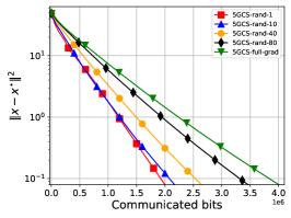
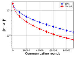
(a)	(b)

Figure 1: (a) Performance of Algorithm 1 (5GCS-CC) with different levels of sparsification $k$. (b) Comparison of Algorithm 2 (5GCS-AB) with uniform sampling and Multisampling in case of $C=1$.

5.3 Uniform Sampling

In this section we show that previous result of  Grudzień et al. (2023) can be covered by our framework. This means we fully generalize previous convergence guarantees. In this case we utilize uniform sampling without replacement.

Theorem 5.9.

Consider Algorithm 2 with uniform sampling scheme satisfying 2 and LT solver satisfying Assumption 3. Let the inequality hold $\frac{1}{{\tau}_{m}}-{\gamma}{M}\geq\frac{4}{{\tau}_{m}^{2}}\frac{\mu}{3M}$, e.g. ${\tau}_{m}\geq\frac{8\mu}{3{M}}$ and ${\gamma}\leq\frac{1}{2{\tau}_{m}{M}}$. Then for the Lyapunov function

$$\Psi^{t}\coloneqq\frac{1}{{\gamma}}\left\|x^{t+1}-x^{\star}\right\|^{2}+\sum_{m=1}^{M}\frac{{M}}{{C}}\left(\frac{1}{{\tau}_{m}}+\frac{1}{L_{F_{m}}}\right)\left\|u_{m}^{t+1}-u_{m}^{\star}\right\|^{2},$$

the iterates of the method satisfy

$$\mathbb{E}\!\left[\Psi^{t+1}\right]\leq\max\left\{\frac{1}{1+{\gamma}\mu},\max_{m}\left[\frac{L_{F_{m}}+\frac{{M}-{C}}{{M}}{\tau}_{m}}{L_{F_{m}}+{\tau}_{m}}\right]\right\}\mathbb{E}\!\left[\Psi^{t}\right].$$

Corollary 5.10.

Suppose that $L_{m}=L,\forall m\in\left\{1,\ldots,{M}\right\}$. Choose any $0<\varepsilon<1$ and ${\gamma}=\frac{3}{16}\sqrt{\frac{{C}}{L\mu{M}}}$ and ${\tau}_{m}=\frac{8}{3}\sqrt{\frac{L\mu}{{M}{C}}}$. In order to guarantee $\mathbb{E}\!\left[\Psi^{T}\right]\leq\varepsilon\Psi^{0}$, it suffices to take

$$T \geq \max\left\{1+\frac{16}{3}\sqrt{\frac{{M}}{{C}}\frac{L}{\mu}},\frac{{M}}{{C}}+\frac{3}{8}\sqrt{\frac{{M}}{{C}}\frac{L}{\mu}}\right\}\log\frac{1}{\varepsilon}$$

$$= {\mathcal{O}}\left(\left(\frac{{M}}{{C}}+\sqrt{\frac{{M}}{{C}}\frac{L}{\mu}}\right)\log\frac{1}{\varepsilon}\right)$$

communication rounds.

6 Experiments

This study primarily focuses on analyzing the fundamental algorithmic and theoretical aspects of a particular class of algorithms, rather than conducting extensive large-scale experiments. While we acknowledge the importance of such experiments, they fall outside the scope of this work. Instead, we provide illustrative examples and validate our findings through the application of logistic regression to a practical problem setting.

We are considering $\ell_{2}$-regularized logistic regression, which is a mathematical model used for classification tasks. The objective function, denoted as $f(x)$, is defined as follows:

$$f(x)=\frac{1}{MN}\sum_{m=1}^{M}\sum_{i=1}^{N}\log\left(1+e^{-b_{m,i}a_{m,i}^{\top}x}\right)+\frac{\lambda}{2}\|x\|^{2}.$$

In this equation, $a_{m,i}\in\mathbb{R}^{d}$ and $b_{m,i}\in\{-1,+1\}$ represent the data samples and labels, respectively. The variables $M$ and $N$ correspond to the number of clients and the number of data points per client, respectively. The term $\lambda$ is a regularization parameter, and in accordance with Condat et al. (2023), we set $\lambda$, such that we have $\kappa=10^{4}$.

To illustrate our experimental results, we have chosen to focus on a specific case using the "a1a" dataset from the LibSVM library (Chang and Lin, 2011). We have $d=119$, $M=107$ and $N=15$ for this dataset.

For the experiments involving communication compression, we utilized the Rand-$k$ compressor (Mishchenko et al., 2019) with various parameters for sparsification and theoretical stepsizes for the method. Based on the plotted results, it is evident that the optimal choice is achieved when setting $k=1$ and the method without communication compression shows the worst performance. We calculate the number of communicated floats by all clients.

In the experiments conducted to evaluate the Multisampling strategy, we employed the exact version of the parameters outlined in Corollary 5.5. Additionally, we applied a re-scaling procedure to modify the distribution of $L_{m}$ in order to reduce its uniformity. The resulting values were approximately $L_{\min}\approx 1.48$ and $L_{\max}\approx 2\cdot 10^{4}$.

The observed results indicate that the exact solution of determining probabilities and stepsizes., despite not being optimal, outperformed the version with uniform sampling.

Supplementary Materials

Appendix A Basic Inequalities

A.1 Young’s inequalities

For all $x,y\in\mathbb{R}^{d}$ and all $a>0$, we have

$$\langle x,y\rangle\leq\frac{a\left\|x\right\|^{2}}{2}+\frac{\left\|y\right\|^{2}}{2a},$$ (8)

$$\left\|x+y\right\|^{2}\leq 2\left\|x\right\|^{2}+2\left\|y\right\|^{2},$$ (9)

$$\frac{1}{2}\left\|x\right\|^{2}-\left\|y\right\|^{2}\leq\left\|x+y\right\|^{2}.$$ (10)

A.2 Variance decomposition

For a random vector $\mathrm{X}\in\mathbb{R}^{d}$ (with finite second moment) and any $c\in\mathbb{R}^{d}$, the variance of $X$ can be decomposed as

$$\mathbb{E}\!\left[\left\|\mathrm{X}-\mathbb{E}\!\left[\mathrm{X}\right]\right\|^{2}\right]=\mathbb{E}\!\left[\left\|\mathrm{X}-c\right\|^{2}\right]-\left\|\mathbb{E}\!\left[\mathrm{X}\right]-c\right\|^{2}.$$ (11)

A.3 Conic compression variance

An unbiased randomized mapping ${\mathcal{C}}:\mathbb{R}^{d}\to\mathbb{R}^{d}$ has conic variance if there exists $\omega\geq 0$ such that

$$\mathbb{E}\!\left[\left\|\mathcal{C}(x)-x\right\|^{2}\right]\leq\omega\left\|x\right\|^{2}$$ (12)

for all $x\in\mathbb{R}^{d}.$

A.4 Convexity and $L$-smoothness

Suppose $\phi\colon\mathbb{R}^{d}\to\mathbb{R}$ is $L$-smooth and convex. Then

$$\frac{1}{L}\left\|\nabla\phi(x)-\nabla\phi(y)\right\|^{2}\leq\langle\nabla\phi(x)-\nabla\phi(y),x-y\rangle$$ (13)

for all $x,y\in\mathbb{R}^{d}$.

A.5 Dual Problem and Saddle-Point Reformulation

Then the saddle function reformulation of $\left(\ref{lifted_form}\right)$ is:

$$\mathrm{Find}\ (x^{\star},(u_{m}^{\star})_{m=1}^{M})\in\arg\min_{x\in\mathbb{R}^{d}}\max_{u\in\mathbb{R}^{{M}d}}\,\left(\frac{\mu}{2}\left\|x\right\|^{2}+\sum_{m=1}^{M}\left\langle x,u_{m}\right\rangle-\sum_{m=1}^{M}F_{m}^{*}(u_{m})\right).$$ (14)

To ensure well-posedness of these problems, we need to assume that there exists $x^{\star}\in\mathbb{R}^{d}$ s.t.:

$$0=\mu x^{\star}+\sum_{m=1}^{{M}}\nabla F_{m}(x^{\star}).$$ (15)

Which is equivalent to $\left(\ref{lifted_form}\right)$, having a solution, which it does (unique in fact) as each $f_{m}$ is $\mu$-strongly convex. By first order optimality condition $x^{\star}$ and $u^{\star}$ that are solution to $\left(\ref{saddlenew}\right)$, satisfy:

$$\left\{\begin{array}[]{l}0=\mu x^{\star}+\sum_{m=1}^{M}u_{m}^{\star}\\ {{H}}x^{\star}\in\partial F^{*}(u^{\star})\end{array}\right..$$ (16)

Where the latter in $\left(\ref{fooc}\right)$ is equivalent to:

$$\nabla F({{H}}x^{\star})=u^{\star}.$$ (17)

Throughout, this section we will denote by $\mathcal{F}_{t}$ for all $t\geq 0$ the $\sigma$-algebra generated by the collection of $\left(\mathbb{R}^{d}\times\mathbb{R}^{d{M}}\right)$-valued random variables $\left(x^{0},u^{0}\right),\dots,\left(x^{t},u^{t}\right).$

Appendix B Proof of Theorem 5.1

Theorem.

Let Assumption 1 hold. Consider Algorithm 2 with sampling scheme $\mathbf{S}$ satisfying Assumption 2 and LT solvers $\mathcal{A}_{m}$ satisfying Assumption 3. Let the inequality hold $\frac{1}{{\tau}_{m}}-\left({\gamma}\left(1-B\right){M}+{\gamma}\frac{A}{w_{m}}\right)\geq\frac{4}{{\tau}_{m}^{2}}\frac{\mu_{m}}{3M}$, e.g. ${\tau}_{m}\geq\frac{8\mu_{m}}{3{M}}$ and ${\gamma}\leq\frac{1}{2{\tau}_{m}\left(\left(1-B\right){M}+\frac{A}{w_{m}}\right)}$. Then for the Lyapunov function

$$\Psi^{t}\coloneqq\frac{1}{{\gamma}}\left\|x^{t}-x^{\star}\right\|^{2}+\sum_{m=1}^{M}\left(1+q_{m}\right)\left(\frac{1}{{\tau}_{m}}+\frac{1}{L_{F_{m}}}\right)\left\|u_{m}^{t}-u_{m}^{\star}\right\|^{2},$$

the iterates of the method satisfy

$$\mathbb{E}\!\left[\Psi^{t+1}\right]\leq\max\left\{\frac{1}{1+{\gamma}\mu},\max_{m}\left[\frac{L_{F_{m}}+\frac{q_{m}}{1+q_{m}}{\tau}_{m}}{L_{F_{m}}+{\tau}_{m}}\right]\right\}\mathbb{E}\!\left[\Psi^{t}\right],$$

where $q_{m}=\frac{1}{\widehat{p}_{m}}-1$ and $\widehat{p}_{m}$ is probability that $m$-th client is participating.

Proof.

We start from using variance decomposition 11 and Proposition 1 from [Condat and Richtárik, 2021], we obtain

$$\mathbb{E}\!\left[\left\|x^{t+1}-x^{\star}\right\|^{2}\;|\;\mathcal{F}_{t}\right] \overset{(\ref{vardec})}{=} \left\|\mathbb{E}\!\left[x^{t+1}\;|\;\mathcal{F}_{t}\right]-x^{\star}\right\|^{2}+\mathbb{E}\!\left[\left\|x^{t+1}-\mathbb{E}\!\left[x^{t+1}\;|\;\mathcal{F}_{t}\right]\right\|^{2}\;|\;\mathcal{F}_{t}\right]$$ (18)

$$\overset{(\ref{weighted})}{=} \underbrace{\left\|\hat{x}^{t}-x^{\star}-{\gamma}{{H}}^{\top}\left(\bar{u}^{t+1}-u^{t}\right)\right\|^{2}}_{X}-{\gamma}^{2}B\left\|{{H}}^{\top}(\bar{u}^{t+1}-u^{t})\right\|^{2}$$

$$+{\gamma}^{2}\sum_{m=1}^{{M}}\frac{A}{w_{m}}\left\|\bar{u}_{m}^{t+1}-u_{m}^{t}\right\|^{2}.$$

Moreover, using $\left(\ref{fooc}\right)$ and the definition of $\hat{x}^{t}$, we have

$$(1+{\gamma}\mu)\hat{x}^{t}=x^{t}-{\gamma}{{H}}^{\top}u^{t},$$ (19)

$$(1+{\gamma}\mu)x^{\star}=x^{\star}-{\gamma}{{H}}^{\top}u^{\star}.$$ (20)

Using $\left(\ref{opt13}\right)$ and $\left(\ref{opt23}\right)$ we obtain

$$X = \left\|\hat{x}^{t}-x^{\star}\right\|^{2}+{\gamma}^{2}\left\|{{H}}^{\top}\left(\bar{u}^{t+1}-u^{t}\right)\right\|^{2}-2{\gamma}\left\langle\hat{x}^{t}-x^{\star},{{H}}^{\top}\left(\bar{u}^{t+1}-u^{t}\right)\right\rangle$$ (21)

$$\leq (1+{\gamma}\mu)\left\|\hat{x}^{t}-x^{\star}\right\|^{2}+{\gamma}^{2}\left\|{{H}}^{\top}\left(\bar{u}^{t+1}-u^{t}\right)\right\|^{2}$$

$$-2{\gamma}\left\langle\hat{x}^{t}-x^{\star},{{H}}^{\top}\left(\bar{u}^{t+1}-u^{\star}\right)\right\rangle+2{\gamma}\left\langle\hat{x}^{t}-x^{\star},{{H}}^{\top}\left(u^{t}-u^{\star}\right)\right\rangle$$

$$\overset{(\ref{opt13})+(\ref{opt23})}{=} \left\langle x^{t}-x^{\star}-{\gamma}{{H}}^{\top}\left(u^{t}-u^{\star}\right),\hat{x}^{t}-x^{\star}\right\rangle+{\gamma}^{2}\left\|{{H}}^{\top}\left(\bar{u}^{t+1}-u^{t}\right)\right\|^{2}$$

$$-2{\gamma}\left\langle\hat{x}^{t}-x^{\star},{{H}}^{\top}\left(\bar{u}^{t+1}-u^{\star}\right)\right\rangle+\left\langle\hat{x}^{t}-x^{\star},2{\gamma}{{H}}^{\top}\left(u^{t}-u^{\star}\right)\right\rangle$$

$$= \left\langle x^{t}-x^{\star}+{\gamma}{{H}}^{\top}\left(u^{t}-u^{\star}\right),\hat{x}^{t}-x^{\star}\right\rangle+{\gamma}^{2}\left\|{{H}}^{\top}\left(\bar{u}^{t+1}-u^{t}\right)\right\|^{2}$$

$$-2{\gamma}\left\langle\hat{x}^{t}-x^{\star},{{H}}^{\top}\left(\bar{u}^{t+1}-u^{\star}\right)\right\rangle$$

$$\overset{(\ref{opt13})+(\ref{opt23})}{=} \frac{1}{1+{\gamma}\mu}\left\langle x^{t}-x^{\star}+{\gamma}{{H}}^{\top}\left(u^{t}-u^{\star}\right),x^{t}-x^{\star}-{\gamma}{{H}}^{\top}\left(u^{t}-u^{\star}\right)\right\rangle$$

$$+{\gamma}^{2}\left\|{{H}}^{\top}\left(\bar{u}^{t+1}-u^{t}\right)\right\|^{2}-2{\gamma}\left\langle\hat{x}^{t}-x^{\star},{{H}}^{\top}\left(\bar{u}^{t+1}-u^{\star}\right)\right\rangle$$

$$= \frac{1}{1+{\gamma}\mu}\left\|x^{t}-x^{\star}\right\|^{2}-\frac{{\gamma}^{2}}{1+{\gamma}\mu}\left\|{{H}}^{\top}\left(u^{t}-u^{\star}\right)\right\|^{2}$$

$$+{\gamma}^{2}\left\|{{H}}^{\top}\left(\bar{u}^{t+1}-u^{t}\right)\right\|^{2}-2{\gamma}\left\langle\hat{x}^{t}-x^{\star},{{H}}^{\top}\left(\bar{u}^{t+1}-u^{\star}\right)\right\rangle.$$

Combining $\left(\ref{x102}\right)$ and $\left(\ref{long31}\right)$

$$\mathbb{E}\!\left[\left\|x^{t+1}-x^{\star}\right\|^{2}\;|\;\mathcal{F}_{t}\right] \leq \frac{1}{1+{\gamma}\mu}\left\|x^{t}-x^{\star}\right\|^{2}-\frac{{\gamma}^{2}}{1+{\gamma}\mu}\left\|{{H}}^{\top}(u^{t}-u^{\star})\right\|^{2}$$

$$+{\gamma}^{2}(1-B)\left\|{{H}}^{\top}(\bar{u}^{t+1}-u^{t})\right\|^{2}$$

$$-2{\gamma}\left\langle\hat{x}^{t}-x^{\star},{{H}}^{\top}(\bar{u}^{t+1}-u^{\star})\right\rangle$$

$$+{\gamma}^{2}\sum_{m=1}^{{M}}\frac{A}{w_{m}}\left\|\bar{u}_{m}^{t+1}-u_{m}^{t}\right\|^{2}-\frac{{\gamma}\mu}{{M}}\left\|{{H}}\hat{x}^{t}-{{H}}x^{\star}\right\|^{2}.$$

Let $\widehat{p}=\left(\widehat{p}_{1},\ldots,\widehat{p}_{M}\right)$. The update for $u$ may be written as

$$u_{m}^{t+1}=u_{m}^{t}+\widehat{p}_{m}\frac{1}{\widehat{p}_{m}}Bernoulli(\bar{u}_{m}^{t+1}-u^{t}_{m},\widehat{p}_{m}),$$

where $\widehat{p}_{m}$ is the probability that client $m$ participates in the iteration. Firstly note that the update for $u_{m}^{t+1}$ can be written as:

$$u_{m}^{t+1}=u_{m}^{t}+\widehat{p}_{m}\widetilde{\mathcal{R}}_{m}(\bar{u}_{m}^{t+1}-u^{t}_{m},\widehat{p}_{m}),$$

i.e we have a relation of $\frac{1}{1+q_{m}}=\widehat{p}_{m}$ , which obviously makes sense, since the independent, unbiased bernoulli compressor with probability $p_{m}$ has conic variance $q_{m}=\frac{1}{\widehat{p}_{m}}-1$. This leads to

$$u_{m}^{t+1}=u_{m}^{t}+\frac{1}{1+q_{m}}\widetilde{\mathcal{R}}_{m}(\bar{u}_{m}^{t+1}-u^{t}_{m},q_{m}).$$

Using such form, we get

$$\mathbb{E}\!\left[\left\|u_{m}^{t+1}-u_{m}^{\star}\right\|^{2}\;|\;\mathcal{F}_{t}\right] \overset{(\ref{vardec})+(\ref{cvar})}{\leq} \left\|u_{m}^{t}-u_{m}^{\star}+\frac{1}{1+q_{m}}\left(\bar{u}_{m}^{t+1}-u_{m}^{t}\right)\right\|^{2}$$ (22)

$$+\frac{q_{m}}{(1+q_{m})^{2}}\left\|\bar{u}_{m}^{t+1}-u_{m}^{t}\right\|^{2}$$

$$= \frac{q_{m}^{2}}{(1+q_{m})^{2}}\left\|u_{m}^{t}-u_{m}^{\star}\right\|^{2}+\frac{1}{(1+q_{m})^{2}}\left\|\bar{u}_{m}^{t+1}-u_{m}^{\star}\right\|^{2}$$

$$+\frac{2q_{m}}{(1+q_{m})^{2}}\left\langle u_{m}^{t}-u_{m}^{\star},\bar{u}_{m}^{t+1}-u_{m}^{\star}\right\rangle$$

$$+\frac{q_{m}}{(1+q_{m})^{2}}\left\|\bar{u}_{m}^{t+1}-u_{m}^{\star}\right\|^{2}+\frac{q_{m}}{(1+q_{m})^{2}}\left\|u_{m}^{t}-u_{m}^{\star}\right\|^{2}$$

$$-\frac{2q_{m}}{(1+q_{m})^{2}}\left\langle u_{m}^{t}-u_{m}^{\star},\bar{u}_{m}^{t+1}-u_{m}^{\star}\right\rangle$$

$$\leq \frac{1}{1+q_{m}}\left\|\bar{u}_{m}^{t+1}-u_{m}^{\star}\right\|^{2}+\frac{q_{m}}{1+q_{m}}\left\|u_{m}^{t}-u_{m}^{\star}\right\|^{2}.$$

Let us consider the first term in $\left(\ref{newubound2}\right)$:

$$\left\|\bar{u}_{m}^{t+1}-u_{m}^{\star}\right\|^{2} = \left\|(u_{m}^{t}-u_{m}^{\star})+(\bar{u}_{m}^{t+1}-u_{m}^{t})\right\|^{2}$$

$$= \left\|u_{m}^{t}-u_{m}^{\star}\right\|^{2}+\left\|\bar{u}_{m}^{t+1}-u_{m}^{t}\right\|^{2}+2\left\langle u_{m}^{t}-u_{m}^{\star},\bar{u}_{m}^{t+1}-u_{m}^{t}\right\rangle$$

$$= \left\|u_{m}^{t}-u_{m}^{\star}\right\|^{2}+2\left\langle\bar{u}_{m}^{t+1}-u_{m}^{\star},\bar{u}_{m}^{t+1}-u_{m}^{t}\right\rangle-\left\|\bar{u}_{m}^{t+1}-u_{m}^{t}\right\|^{2}.$$

Combining terms together we get

$$\mathbb{E}\!\left[\left\|u_{m}^{t+1}-u_{m}^{\star}\right\|^{2}\;|\;\mathcal{F}_{t}\right] \leq\left\|u_{m}^{t}-u_{m}^{\star}\right\|^{2}$$

$$+\frac{1}{1+q_{m}}\left(2\left\langle\bar{u}_{m}^{t+1}-u_{m}^{\star},\bar{u}_{m}^{t+1}-u_{m}^{t}\right\rangle-\left\|\bar{u}_{m}^{t+1}-u_{m}^{t}\right\|^{2}\right).$$

Finally, we obtain

$$\frac{1}{{\gamma}}\mathbb{E}\!\left[\left\|x^{t+1}-x^{\star}\right\|^{2}\;|\;\mathcal{F}_{t}\right] + \sum_{m=1}^{M}\frac{1+q_{m}}{{\tau}_{m}}\mathbb{E}\!\left[\left\|u_{m}^{t+1}-u_{m}^{\star}\right\|^{2}\;|\;\mathcal{F}_{t}\right]$$

$$\leq \frac{1}{{\gamma}\left(1+{\gamma}\mu\right)}\left\|x^{t}-x^{\star}\right\|^{2}-\frac{{\gamma}}{1+{\gamma}\mu}\left\|{{H}}^{\top}(u^{t}-u^{\star})\right\|^{2}$$

$$+{\gamma}(1-B)\left\|{{H}}^{\top}(\bar{u}^{t+1}-u^{t})\right\|^{2}$$

$$+{\gamma}\sum_{m=1}^{{M}}\frac{A}{w_{m}}\left\|\bar{u}_{m}^{t+1}-u_{m}^{t}\right\|^{2}-\frac{\mu}{{M}}\left\|{{H}}\hat{x}^{t}-{{H}}x^{\star}\right\|^{2}$$

$$+\frac{1+q_{m}}{{\tau}_{m}}\left\|u_{m}^{t}-u_{m}^{\star}\right\|^{2}-2\sum_{m=1}^{M}\left\langle\hat{x}^{t}-x^{\star},\bar{u}_{m}^{t+1}-u_{m}^{\star}\right\rangle$$

$$+\frac{1}{{\tau}_{m}}\left(2\left\langle\bar{u}_{m}^{t+1}-u_{m}^{\star},\bar{u}_{m}^{t+1}-u_{m}^{t}\right\rangle-\left\|\bar{u}_{m}^{t+1}-u_{m}^{t}\right\|^{2}\right).$$

Ignoring $-\frac{{\gamma}}{1+{\gamma}\mu}\left\|{{H}}^{\top}(u^{t}-u^{\star})\right\|^{2}$ and noting

$$-\left\langle\hat{x}^{t}-x^{\star},\bar{u}_{m}^{t+1}-u_{m}^{\star}\right\rangle+\frac{1}{{\tau}_{m}}\left\langle\bar{u}_{m}^{t+1}-u_{m}^{\star},\bar{u}_{m}^{t+1}-u_{m}^{t}\right\rangle$$

$$=-\left\langle y_{m}^{K,t}-x^{\star},\bar{u}_{m}^{t+1}-u_{m}^{\star}\right\rangle+\frac{1}{{\tau}_{m}}\left\langle\nabla\psi^{t}_{m}(y_{m}^{K,t}),\bar{u}_{m}^{t+1}-u_{m}^{\star}\right\rangle$$

$$\overset{(\ref{yi1})+(\ref{strmono})}{\leq}-\frac{1}{L_{F_{m}}}\left\|\bar{u}_{m}^{t+1}-u_{m}^{\star}\right\|^{2}+\frac{a_{m}}{2{\tau}_{m}}\left\|\nabla\psi^{t}_{m}(y_{m}^{K,t})\right\|^{2}+\frac{1}{2a_{m}{\tau}_{m}}\left\|\bar{u}_{m}^{t+1}-u_{m}^{\star}\right\|^{2}$$

$$=-\left(\frac{1}{L_{F_{m}}}-\frac{1}{2a_{m}{\tau}_{m}}\right)\left\|\bar{u}_{m}^{t+1}-u_{m}^{\star}\right\|^{2}+\frac{a_{m}}{2{\tau}_{m}}\left\|\nabla\psi^{t}_{m}(y_{m}^{K,t})\right\|^{2}$$

$$\overset{(\ref{newubound2})}{\leq}-\left(\frac{1}{L_{F_{m}}}-\frac{1}{2a_{m}{\tau}_{m}}\right)\left(\left(1+q_{m}\right)\mathbb{E}\!\left[\left\|u_{m}^{t+1}-u_{m}^{\star}\right\|^{2}\;|\;\mathcal{F}_{t}\right]-q_{m}\left\|u_{m}^{t}-u_{m}^{\star}\right\|^{2}\right)$$

$$+\frac{a_{m}}{2{\tau}_{m}}\left\|\nabla\psi^{t}_{m}(y_{m}^{K,t})\right\|^{2},$$

we get

$$\frac{1}{{\gamma}}\mathbb{E}\!\left[\left\|x^{t+1}-x^{\star}\right\|^{2}\;|\;\mathcal{F}_{t}\right] + \sum_{m=1}^{M}\left(1+q_{m}\right)\left(\frac{1}{{\tau}_{m}}+\frac{1}{L_{F_{m}}}\right)\mathbb{E}\!\left[\left\|u_{m}^{t+1}-u_{m}^{\star}\right\|^{2}\;|\;\mathcal{F}_{t}\right]$$

$$\leq \frac{1}{{\gamma}\left(1+{\gamma}\mu\right)}\left\|x^{t}-x^{\star}\right\|^{2}$$

$$+ \sum_{m=1}^{M}\left(1+q_{m}\right)\left(\frac{1}{{\tau}_{m}}+\frac{q_{m}}{1+q_{m}}\frac{1}{L_{F_{m}}}\right)\left\|u_{m}^{t}-u_{m}^{\star}\right\|^{2}$$

$$+\sum_{m=1}^{M}\left({\gamma}\left(1-B\right){M}+{\gamma}\frac{A}{w_{m}}-\frac{1}{{\tau}_{m}}\right)\left\|\bar{u}_{m}^{t+1}-u_{m}^{t}\right\|^{2}$$

$$+\sum_{m=1}^{M}\frac{L_{F_{m}}}{{\tau}_{m}^{2}}\left\|\nabla\psi^{t}_{m}(y_{m}^{K,t})\right\|^{2}-\sum_{m=1}^{M}\mu v_{m}\left\|\hat{x}^{t}-x^{\star}\right\|^{2}.$$

Where we made the choice $a_{m}=\frac{L_{F_{m}}}{\tau_{m}}$ and $\sum_{m=1}^{M}v_{m}\leq 1$, positive real numbers, e.g. $\frac{\mu_{m}}{\sum_{m=1}^{M}\mu_{m}}$. Using Young’s inequality we have

$$-\frac{\mu v_{m}}{3}\left\|\hat{x}^{t}-y_{m}^{\star,t}+y_{m}^{\star,t}-x^{\star}\right\|^{2}\overset{(\ref{yi3})}{\leq}\frac{\mu v_{m}}{3}\left\|y_{m}^{\star,t}-x^{\star}\right\|^{2}-\frac{\mu v_{m}}{6}\left\|\hat{x}^{t}-y_{m}^{\star,t}\right\|^{2}.$$

Noting the fact that $y_{m}^{\star,t}=\hat{x}^{t}-\frac{1}{{\tau}_{m}}(\hat{u}_{m}^{t+1}-u_{m}^{t})$, we have

$$\frac{\mu v_{m}}{3}\left\|y_{m}^{\star,t}-x^{\star}\right\|^{2}\overset{(\ref{yi2})}{\leq}2\frac{\mu v_{m}}{3}\left\|\hat{x}^{t}-x^{\star}\right\|^{2}+\frac{2}{{\tau}_{m}^{2}}\frac{\mu v_{m}}{3}\left\|\hat{u}_{m}^{t+1}-u_{m}^{t}\right\|^{2}.$$

Combining those inequalities we get

$$\frac{1}{{\gamma}}\mathbb{E}\!\left[\left\|x^{t+1}-x^{\star}\right\|^{2}\;|\;\mathcal{F}_{t}\right] + \sum_{m=1}^{M}\left(1+q_{m}\right)\left(\frac{1}{{\tau}_{m}}+\frac{1}{L_{F_{m}}}\right)\mathbb{E}\!\left[\left\|u_{m}^{t+1}-u_{m}^{\star}\right\|^{2}\;|\;\mathcal{F}_{t}\right]$$

$$\leq \frac{1}{{\gamma}\left(1+{\gamma}\mu\right)}\left\|x^{t}-x^{\star}\right\|^{2}$$

$$+\sum_{m=1}^{M}\left(1+q_{m}\right)\left(\frac{1}{{\tau}_{m}}+\frac{q_{m}}{1+q_{m}}\frac{1}{L_{F_{m}}}\right)\left\|u_{m}^{t}-u_{m}^{\star}\right\|^{2}$$

$$+\sum_{m=1}^{M}\frac{2}{{\tau}_{m}^{2}}\frac{\mu v_{m}}{3}\left\|\hat{u}_{m}^{t+1}-u_{m}^{t}\right\|^{2}$$

$$-\sum_{m=1}^{M}\left(\frac{1}{{\tau}_{m}}-\left({\gamma}\left(1-B\right){M}+{\gamma}\frac{A}{w_{m}}\right)\right)\left\|\bar{u}_{m}^{t+1}-u_{m}^{t}\right\|^{2}$$

$$+\sum_{m=1}^{M}\frac{L_{F_{m}}}{{\tau}_{m}^{2}}\left\|\nabla\psi^{t}_{m}(y_{m}^{K,t})\right\|^{2}-\sum_{m=1}^{M}\frac{\mu v_{m}}{6}\left\|\hat{x}^{t}-y_{m}^{\star,t}\right\|^{2}.$$

Assuming ${\gamma}$ and ${\tau}_{m}$ can be chosen so that $\frac{1}{{\tau}_{m}}-\left({\gamma}\left(1-B\right){M}+{\gamma}\frac{A}{w_{m}}\right)\geq\frac{4}{{\tau}_{m}^{2}}\frac{\mu v_{m}}{3}$ we obtain

$$\frac{1}{{\gamma}}\mathbb{E}\!\left[\left\|x^{t+1}-x^{\star}\right\|^{2}\;|\;\mathcal{F}_{t}\right] + \sum_{m=1}^{M}\left(1+q_{m}\right)\left(\frac{1}{{\tau}_{m}}+\frac{1}{L_{F_{m}}}\right)\mathbb{E}\!\left[\left\|u_{m}^{t+1}-u_{m}^{\star}\right\|^{2}\;|\;\mathcal{F}_{t}\right]$$

$$\leq \frac{1}{{\gamma}\left(1+{\gamma}\mu\right)}\left\|x^{t}-x^{\star}\right\|^{2}$$

$$+\sum_{m=1}^{M}\left(1+q_{m}\right)\left(\frac{1}{{\tau}_{m}}+\frac{q_{m}}{1+q_{m}}\frac{1}{L_{F_{m}}}\right)\left\|u_{m}^{t}-u_{m}^{\star}\right\|^{2}$$

$$+\sum_{m=1}^{M}\frac{4}{{\tau}_{m}^{2}}\frac{\mu v_{m}L_{F_{m}}^{2}}{3}\left\|y_{m}^{K,t}-y_{m}^{\star,t}\right\|^{2}$$

$$+\sum_{m=1}^{M}\frac{L_{F_{m}}}{{\tau}_{m}^{2}}\left\|\nabla\psi^{t}_{m}(y_{m}^{K,t})\right\|^{2}-\sum_{m=1}^{M}\frac{\mu v_{m}}{6}\left\|\hat{x}^{t}-y_{m}^{\star,t}\right\|^{2}.$$

The point $y^{K,t}$ is supposed to satisfy Assumption 3:

$$\sum_{m=1}^{M}\frac{4}{{\tau}_{m}^{2}}\frac{\mu v_{m}L^{2}_{F_{m}}}{3}\left\|y_{m}^{K,t}-y_{m}^{\star,t}\right\|^{2}+\sum_{m=1}^{M}\frac{L_{F_{m}}}{{\tau}_{m}^{2}}\left\|\nabla\psi^{t}_{m}(y_{m}^{K,t})\right\|^{2}\leq\sum_{m=1}^{M}\frac{\mu v_{m}}{6}\left\|\hat{x}^{t}-y_{m}^{\star,t}\right\|^{2}.$$

Thus

$$\frac{1}{{\gamma}}\mathbb{E}\!\left[\left\|x^{t+1}-x^{\star}\right\|^{2}\;|\;\mathcal{F}_{t}\right] + \sum_{m=1}^{M}\left(1+q_{m}\right)\left(\frac{1}{{\tau}_{m}}+\frac{1}{L_{F_{m}}}\right)\mathbb{E}\!\left[\left\|u_{m}^{t+1}-u_{m}^{\star}\right\|^{2}\;|\;\mathcal{F}_{t}\right]$$

$$\leq \frac{1}{{\gamma}\left(1+{\gamma}\mu\right)}\left\|x^{t}-x^{\star}\right\|^{2}$$

$$+\sum_{m=1}^{M}\left(1+q_{m}\right)\left(\frac{1}{{\tau}_{m}}+\frac{q_{m}}{1+q_{m}}\frac{1}{L_{F_{m}}}\right)\left\|u_{m}^{t}-u_{m}^{\star}\right\|^{2}.$$

By taking the expectation on both sides we get

$$\mathbb{E}\!\left[\Psi^{t+1}\right]\leq\max\left\{\frac{1}{1+{\gamma}\mu},\frac{L_{F_{m}}+\frac{q_{m}}{1+q_{m}}{\tau}_{m}}{L_{F_{m}}+{\tau}_{m}}\right\}\mathbb{E}\!\left[\Psi^{t}\right],$$

which finishes the proof. ∎

Appendix C Multisampling (Sampling with Replacement)

C.1 Proof of Lemma 5.2

Lemma.

The Multisampling with estimator 5 satisfies the Assumption 2 with $A=B=\frac{1}{C}$ and $w_{m}=p_{m}$.

Proof.

The proof is presented in Tyurin et al. [2022a]. Let us provide it for completeness.

Let us fix ${C}>0$. For all $m\in[{C}]$, we define i.i.d. random variables

$$\mathcal{X}_{m}=\begin{cases}1&\text{with probability }p_{1}\\ 2&\text{with probability }p_{2}\\ &\cdot\\ &\cdot\\ &\cdot\\ {M}&\text{with probability }p_{M},\end{cases}$$

where $\underline{p}=\left(p_{1},\ldots,p_{M}\right)\in\Delta^{M}$(simple simplex). A sampling

$$S(a_{1},\ldots,a_{M};\underline{p})\coloneqq\frac{1}{{C}}\sum_{m=1}^{{C}}\frac{a_{\mathcal{X}_{m}}}{{M}p_{\mathcal{X}_{m}}}$$

is called the Importance sampling.

Let us establish inequality for Assumption 2:

$$\mathbb{E}\!\left[\left\|\frac{1}{{C}}\sum_{m=1}^{{C}}\frac{a_{\mathcal{X}_{m}}}{{M}p_{\mathcal{X}_{m}}}-\frac{1}{{M}}\sum_{m=1}^{{M}}a_{m}\right\|^{2}\right]=\frac{1}{{C}^{2}}\sum_{m=1}^{{C}}\mathbb{E}\!\left[\left\|\frac{a_{\mathcal{X}_{m}}}{{M}p_{\mathcal{X}_{m}}}-\frac{1}{{M}}\sum_{m=1}^{{M}}a_{m}\right\|^{2}\right]$$

$$+\frac{1}{{C}^{2}}\sum_{m\neq m^{\prime}}\mathbb{E}\!\left[\left\langle\frac{a_{\mathcal{X}_{m}}}{{M}p_{\mathcal{X}_{m}}}-\frac{1}{{M}}\sum_{m=1}^{{M}}a_{m},\frac{a_{\mathcal{X}_{m}^{\prime}}}{{M}p_{\mathcal{X}_{m}^{\prime}}}-\frac{1}{{M}}\sum_{m=1}^{{M}}a_{m}\right\rangle\right].$$

By utilizing the independence and unbiasedness of the random variables, the final term becomes zero, resulting in:

$$\mathbb{E}\!\left[\left\|\frac{1}{{C}}\sum_{m=1}^{{C}}\frac{a_{\mathcal{X}_{m}}}{{M}p_{\mathcal{X}_{m}}}-\frac{1}{{M}}\sum_{m=1}^{{M}}a_{m}\right\|^{2}\right] = \frac{1}{{C}^{2}}\sum_{m=1}^{{C}}\mathbb{E}\!\left[\left\|\frac{a_{\mathcal{X}_{m}}}{{M}p_{\mathcal{X}_{m}}}-\frac{1}{{M}}\sum_{m=1}^{{M}}a_{m}\right\|^{2}\right]$$

$$= \frac{1}{{C}^{2}}\sum_{m=1}^{{C}}\mathbb{E}\!\left[\left\|\frac{a_{\mathcal{X}_{m}}}{{M}p_{\mathcal{X}_{m}}}\right\|^{2}\right]-\frac{1}{{C}}\left\|\frac{1}{{M}}\sum_{m=1}^{{M}}a_{m}\right\|^{2}$$

$$= \frac{1}{{C}}\sum_{m=1}^{{M}}p_{m}\left\|\frac{a_{m}}{{M}p_{m}}\right\|^{2}-\frac{1}{{C}}\left\|\frac{1}{{M}}\sum_{m=1}^{{M}}a_{m}\right\|^{2}$$

$$= \frac{1}{{C}}\left(\frac{1}{{M}}\sum_{m=1}^{{M}}\frac{1}{{M}p_{m}}\left\|a_{m}\right\|^{2}-\left\|\frac{1}{{M}}\sum_{m=1}^{{M}}a_{m}\right\|^{2}\right).$$

Thus we have $A=B=\frac{1}{{C}}$. ∎

C.2 Proof of Theorem 5.3

Theorem.

Let Assumption 1 hold. Consider Algorithm 2 (5GCS-AB) with Multisampling and estimator 5 satisfying Assumption 2 and LT solvers $\mathcal{A}_{m}$ satisfying Assumption 3. Let the inequality hold $\frac{1}{{\tau}_{m}}-\left({\gamma}\left(1-\frac{1}{{C}}\right){M}+{\gamma}\frac{1}{{C}p_{m}}\right)\geq\frac{4}{{\tau}_{m}^{2}}\frac{\mu_{m}}{3{M}}$ , e.g. ${\tau}_{m}\geq\frac{8\mu_{m}}{3{M}}$ and ${\gamma}\leq\frac{1}{2{\tau}_{m}\left(\left(1-\frac{1}{{C}}\right){M}+\frac{1}{{C}p_{m}}\right)}$. Then for the Lyapunov function

$$\Psi^{t}\coloneqq\frac{1}{{\gamma}}\left\|x^{t}-x^{\star}\right\|^{2}+\sum_{m=1}^{M}\frac{1}{\widehat{p}_{m}}\left(\frac{1}{{\tau}_{m}}+\frac{1}{L_{F_{m}}}\right)\left\|u_{m}^{t}-u_{m}^{\star}\right\|^{2},$$

the iterates of the method satisfy

$$\mathbb{E}\!\left[\Psi^{t+1}\right]\leq\max\left\{\frac{1}{1+{\gamma}\mu},\max_{m}\left[\frac{L_{F_{m}}+\left(1-\widehat{p}_{m}\right){\tau}_{m}}{L_{F_{m}}+{\tau}_{m}}\right\}\right]\mathbb{E}\!\left[\Psi^{t}\right],$$

where $\widehat{p}_{m}=1-\left(1-p_{m}\right)^{C}$ is probability that $m$-th client is participating.

Proof.

We start from theorem 5.1:

$$\mathbb{E}\!\left[\Psi^{t+1}\right]\leq\max\left\{\frac{1}{1+{\gamma}\mu},\frac{L_{F_{m}}+\frac{q_{m}}{1+q_{m}}{\tau}_{m}}{L_{F_{m}}+{\tau}_{m}}\right\}\mathbb{E}\!\left[\Psi^{t}\right].$$

For Multisampling the probability of $m$-th client participating is $\widehat{p}_{m}=1-\left(1-p_{m}\right)^{C}$ and we have relation $\widehat{p}_{m}=\frac{1}{1+q_{m}}$. Plugging $q_{m}=\frac{1}{\widehat{p}_{m}}-1$ into recursion gives us

$$\mathbb{E}\!\left[\Psi^{t+1}\right]\leq\max\left\{\frac{1}{1+{\gamma}\mu},\max_{m}\left[\frac{L_{F_{m}}+\left(1-\widehat{p}_{m}\right){\tau}_{m}}{L_{F_{m}}+{\tau}_{m}}\right\}\right]\mathbb{E}\!\left[\Psi^{t}\right].$$

Also using Lemma 5.2 we have $A=B=\frac{1}{C}$ and $w=p_{m}$. Plugging such constants to inequality for $\gamma$ and $\tau_{m}$ leads to $\frac{1}{{\tau}_{m}}-\left({\gamma}\left(1-\frac{1}{{C}}\right){M}+{\gamma}\frac{1}{{C}p_{m}}\right)\geq\frac{4}{{\tau}_{m}^{2}}\frac{\mu_{m}}{3{M}}$ , e.g. ${\tau}_{m}\geq\frac{8\mu_{m}}{3{M}}$ and ${\gamma}\leq\frac{1}{2{\tau}_{m}\left(\left(1-\frac{1}{{C}}\right){M}+\frac{1}{{C}p_{m}}\right)}$. ∎

C.3 Proof of Corollary 5.4

Corollary.

Suppose ${C}=1$. Choose any $0<\varepsilon<1$ and $p_{m}=\frac{\sqrt{L_{F,m}+{\tau}_{m}}}{\sum_{m=1}^{M}\sqrt{L_{F,m}+{\tau}_{m}}}$, and ${\tau}_{m}=\frac{8}{3}\sqrt{\overline{L}\mu{M}}p_{m}$. In order to guarantee $\mathbb{E}\!\left[\Psi^{T}\right]\leq\varepsilon\Psi^{0}$, it suffices to take

$$T\geq\max\left\{1+\frac{16}{3}\sqrt{\frac{\overline{L}{M}}{\mu}},\frac{3}{8}\sqrt{\frac{\overline{L}{M}}{\mu}}+{M}\right\}\log\frac{1}{\varepsilon}$$

communication rounds.

Proof.

We set parameters as $p_{m}=\frac{\sqrt{L_{F_{m}}+{\tau}_{m}}}{\sum_{m=1}^{M}\sqrt{L_{F_{m}}+{\tau}_{m}}}$, and ${\tau}_{m}=\frac{8}{3}\sqrt{\overline{L}\mu{M}}p_{m}$. Let us derive the communication complexity:

$$T \geq\max\left\{1+\frac{16}{3}\sqrt{\frac{\overline{L}{M}}{\mu}},\frac{3}{8}\sqrt{\frac{\overline{L}{M}}{\mu}}+{M}\right\}\log\frac{1}{\varepsilon}$$

$$\geq\max\left\{1+\frac{16}{3}\sqrt{\frac{\overline{L}{M}}{\mu}},\frac{3}{8}\frac{{M}\overline{L}+{M}\frac{8}{3}\sqrt{\overline{L}\mu{M}}}{\sqrt{\overline{L}\mu{M}}}\right\}\log\frac{1}{\varepsilon}$$

$$\geq\max\left\{1+\frac{16}{3}\sqrt{\frac{\overline{L}{M}}{\mu}},\frac{3}{8}\frac{\left(\sum_{m=1}^{M}\sqrt{L_{F_{m}+{\tau}_{m}}}\right)^{2}}{\sqrt{\overline{L}\mu{M}}}\right\}\log\frac{1}{\varepsilon}$$

$$\geq\max\left\{1+\frac{16}{3}\sqrt{\frac{\overline{L}{M}}{\mu}},\max_{m}\left(\frac{3}{8}\frac{\left(\sum_{m=1}^{M}\sqrt{L_{F_{m}+{\tau}_{m}}}\right)^{2}}{\left(L_{F_{m}}+{\tau}_{m}\right)\sqrt{\overline{L}\mu{M}}}\left(L_{F_{m}}+{\tau}_{m}\right)\right)\right\}\log\frac{1}{\varepsilon}.$$

Unrolling the recursion from Theorem 5.3 we get

$$\mathbb{E}\!\left[\Psi^{T}\right]\leq\left(\max\left\{\frac{1}{1+{\gamma}\mu},\max_{m}\left[\frac{L_{F_{m}}+\left(1-\widehat{p}_{m}\right){\tau}_{m}}{L_{F_{m}}+{\tau}_{m}}\right\}\right]\right)^{T}\Psi^{0}.$$ (23)

Using Lemma from Malinovsky et al. [2021] for recursion (Appendix B), we can state that derived $T$ is sufficient to guarantee 23.

C.4 Proof of Corollary 5.5

Corollary.

Suppose $C=1$. Choose any $0<\varepsilon<1$ and $p_{m}=\frac{\sqrt{\frac{L_{m}}{{M}}}}{\sum_{m=1}^{M}\sqrt{\frac{L_{m}}{{M}}}}$, and ${\tau}_{m}=\frac{8}{3}\sqrt{\overline{L}\mu{M}}p_{m}$. In order to guarantee $\mathbb{E}\!\left[\Psi^{T}\right]\leq\varepsilon\Psi^{0}$, it suffices to take

$$T\geq\max\left\{1+\frac{16}{3}\sqrt{\frac{\overline{L}{M}}{\mu}},\frac{3}{8}\sqrt{\frac{\overline{L}{M}}{\mu}}+\frac{\sum_{m=1}^{M}\sqrt{L_{m}}}{\sqrt{L_{\min}}}\right\}\log\frac{1}{\varepsilon}$$

communication rounds. Note that $L_{\min}=\min_{m}L_{m}$.

We set parameters as $p_{m}=\frac{\sqrt{\frac{L_{m}}{{M}}}}{\sum_{m=1}^{M}\sqrt{\frac{L_{m}}{{M}}}}$, and ${\tau}_{m}=\frac{8}{3}\sqrt{\overline{L}\mu{M}}p_{m}$. Let us derive the communication complexity. Since $\left(\sum_{m=1}^{M}\sqrt{\frac{L_{m}}{{M}}}\right)^{2}\leq{M}\overline{L}$ we have

$$T \geq\max\left\{1+\frac{16}{3}\sqrt{\frac{\overline{L}{M}}{\mu}},\frac{3}{8}\sqrt{\frac{\overline{L}{M}}{\mu}}+\frac{\sum_{m=1}^{M}\sqrt{L_{m}}}{\sqrt{L_{\min}}}\right\}\log\frac{1}{\varepsilon}$$

$$\geq\max\left\{1+\frac{16}{3}\sqrt{\frac{\overline{L}{M}}{\mu}},\frac{3}{8}\frac{\left(\sum_{m=1}^{M}\sqrt{\frac{L_{m}}{{M}}}\right)^{2}}{\sqrt{\overline{L}\mu{M}}}+\frac{\sum_{m=1}^{M}\sqrt{\frac{L_{m}}{{M}}}}{\sqrt{\frac{L_{\min}}{{M}}}}\right\}\log\frac{1}{\varepsilon}$$

$$\geq\max\left\{1+\frac{16}{3}\sqrt{\frac{\overline{L}{M}}{\mu}},\max_{m}\left(\frac{3}{8}\frac{\left(\sum_{m=1}^{M}\sqrt{\frac{L_{m}}{{M}}}\right)^{2}}{\frac{L_{m}}{{M}}\sqrt{L^{+}\mu{M}}}\frac{L_{m}-\mu_{m}}{{M}}+\frac{\sum_{m=1}^{M}\sqrt{\frac{L_{m}}{{M}}}}{\sqrt{\frac{L_{m}}{{M}}}}\right)\right\}\log\frac{1}{\varepsilon}$$

$$\geq\max\left\{1+\frac{1}{{\gamma}\mu},\max_{m}\left(\frac{1}{\widehat{p}_{m}}\left(\frac{L_{F_{m}}}{{\tau}_{m}}+1\right)\right)\right\}\log\frac{1}{\varepsilon}$$

$$\geq\max\left\{1+\frac{1}{{\gamma}\mu},\max_{m}\left(\left(1+q_{m}\right)\left(\frac{L_{F_{m}}}{{\tau}_{m}}+1\right)\right)\right\}\log\frac{1}{\varepsilon}.$$

Unrolling the recursion from Theorem 5.3 we get

$$\mathbb{E}\!\left[\Psi^{T}\right]\leq\left(\max\left\{\frac{1}{1+{\gamma}\mu},\max_{m}\left[\frac{L_{F_{m}}+\left(1-\widehat{p}_{m}\right){\tau}_{m}}{L_{F_{m}}+{\tau}_{m}}\right\}\right]\right)^{T}\Psi^{0}.$$ (24)

Using Lemma from Malinovsky et al. [2021] for recursion (Appendix B), we can state that derived $T$ is sufficient to guarantee 24. ∎

Appendix D Independent Sampling (Sampling without Replacement)

D.1 Proof of Lemma 5.6

Lemma.

The Independent Sampling with estimator 7 satisfies the Assumption 2 with $A=\frac{1}{\sum_{m}^{M}\frac{p_{m}}{1-p_{m}}}$, $B=0$ and $w_{m}=\frac{\frac{p_{m}}{1-p_{m}}}{\sum_{m=1}^{M}\frac{p_{m}}{1-p_{m}}}$.

Proof.

The proof is presented in Tyurin et al. [2022a]. Let us provide it for completeness.

Let us define i.i.d. random variables

$$\chi_{m}=\begin{cases}1&\text{with probability }p_{m}\\ 0&\text{with probability }1-p_{m},\end{cases}$$

for all $m\in[M]$, also take $S^{t}\coloneqq\left\{m\in[M]|\chi_{m}=1\right\}$ and $\underline{p}=\left(p_{1},\ldots,p_{M}\right)$ . The corresponding estimator for this sampling has the following form:

$$S(a_{1},\ldots,a_{M},\psi,\underline{p})\coloneqq\frac{1}{{M}}\sum_{m\in S}\frac{a_{m}}{p_{m}}.$$ (25)

We get

$$\mathrm{E}\left[\left\|\frac{1}{M}\sum_{m\in S}\frac{a_{m}}{p_{m}}-\frac{1}{M}\sum_{m=1}^{M}a_{m}\right\|^{2}\right] =\mathrm{E}\left[\left\|\frac{1}{M}\sum_{m=1}^{M}\frac{1}{p_{m}}\chi_{m}a_{m}\right\|^{2}\right]-\left\|\frac{1}{M}\sum_{m=1}^{M}a_{m}\right\|^{2}$$

$$=\sum_{m=1}^{M}\frac{\mathrm{E}\left[\chi_{m}\right]}{M^{2}p_{m}^{2}}\left\|a_{m}\right\|^{2}+\sum_{m\neq k}\frac{\mathrm{E}\left[\chi_{m}\right]\mathrm{E}\left[\chi_{k}\right]}{M^{2}p_{m}p_{k}}\left\langle a_{m},a_{k}\right\rangle$$

$$-\left\|\frac{1}{M}\sum_{m=1}^{M}a_{m}\right\|^{2}$$

$$=\sum_{m=1}^{M}\frac{1}{M^{2}p_{m}}\left\|a_{m}\right\|^{2}+\frac{1}{M^{2}}\left(\left\|\sum_{m=1}^{M}a_{m}\right\|^{2}-\sum_{m=1}^{M}\left\|a_{m}\right\|^{2}\right)$$

$$-\left\|\frac{1}{M}\sum_{m=1}^{M}a_{m}\right\|^{2}$$

$$=\frac{1}{M^{2}}\sum_{m=1}^{M}\left(\frac{1}{p_{m}}-1\right)\left\|a_{m}\right\|^{2}.$$

Thus we have $A=\frac{1}{\sum_{m=1}^{M}\frac{p_{m}}{1-p_{m}}},B=0$ and $w_{m}=\frac{\frac{p_{n}}{1-p_{m}}}{\sum_{m=1}^{M}\frac{p_{m}}{1-p_{m}}}$ for all $m\in[M]$. ∎

D.2 Proof of Theorem 5.7

Theorem.

Consider Algorithm 2 with Independent Sampling with estimator 7 satisfying Assumption 2 and LT solver satisfying Assumption 3. Let the inequality hold $\frac{1}{{\tau}_{m}}-\left({\gamma}{M}+{\gamma}\frac{1-p_{m}}{p_{m}}\right)\geq\frac{4}{{\tau}_{m}^{2}}\frac{\mu_{m}}{3M}$, e.g. ${\tau}_{m}\geq\frac{8\mu_{m}}{3{M}}$ and ${\gamma}\leq\frac{1}{2{\tau}_{m}\left({M}+\frac{1-p_{m}}{p_{m}}\right)}$. Then for the Lyapunov function

$$\Psi^{t}\coloneqq\frac{1}{{\gamma}}\left\|x^{t+1}-x^{\star}\right\|^{2}+\sum_{m=1}^{M}\frac{1}{p_{m}}\left(\frac{1}{{\tau}_{m}}+\frac{1}{L_{F_{m}}}\right)\left\|u_{m}^{t+1}-u_{m}^{\star}\right\|^{2},$$

the iterates of the method satisfy

$$\mathbb{E}\!\left[\Psi^{t+1}\right]\leq\max\left\{\frac{1}{1+{\gamma}\mu},\max_{m}\left[\frac{L_{F_{m}}+\left(1-p_{m}\right){\tau}_{m}}{L_{F_{m}}+{\tau}_{m}}\right]\right\}\mathbb{E}\!\left[\Psi^{t}\right],$$

where $p_{m}$ is probability that $m$-th client is participating.

Proof.

Using Lemma 5.6 we have $A=\frac{1}{\sum_{m=1}^{M}\frac{p_{m}}{1-p_{m}}},B=0$ and $w_{m}=\frac{\frac{p_{n}}{1-p_{m}}}{\sum_{m=1}^{M}\frac{p_{m}}{1-p_{m}}}$ for all $m\in[M]$. Using Theorem 5.1 and we plug this constants into

$$\mathbb{E}\!\left[\Psi^{t+1}\right]\leq\max\left\{\frac{1}{1+{\gamma}\mu},\frac{L_{F_{m}}+\frac{q_{m}}{1+q_{m}}{\tau}_{m}}{L_{F_{m}}+{\tau}_{m}}\right\}\mathbb{E}\!\left[\Psi^{t}\right],$$

and we obtain

$$\mathbb{E}\!\left[\Psi^{t+1}\right]\leq\max\left\{\frac{1}{1+{\gamma}\mu},\max_{m}\left[\frac{L_{F_{m}}+\left(1-p_{m}\right){\tau}_{m}}{L_{F_{m}}+{\tau}_{m}}\right]\right\}\mathbb{E}\!\left[\Psi^{t}\right].$$

∎

D.3 Proof of Corollary 5.8

Corollary D.1.

Choose any $0<\varepsilon<1$ and $p_{m}$ can be estimated but not set, then set ${\tau}_{m}=\frac{8}{3}\sqrt{\frac{\bar{L}\mu}{M\sum_{m=1}^{M}p_{m}}}$ and ${\gamma}=\frac{1}{2{\tau}_{m}\left({M}+\frac{1-p_{m}}{p_{m}}\right)}$. In order to guarantee $\mathbb{E}\!\left[\Psi^{T}\right]\leq\varepsilon\Psi^{0}$, it suffices to take

$$T\geq\max\left\{1+\frac{16}{3}\sqrt{\frac{\overline{L}{M}}{\mu\sum_{m=1}^{M}p_{m}}}\left(1+\frac{1}{{M}}\frac{1-p_{m}}{p_{m}}\right),\max_{m}\left[\frac{3}{8}\frac{L_{F_{m}}}{p_{m}}\sqrt{\frac{{M}\sum_{m=1}^{M}p_{m}}{\overline{L}\mu}}+\frac{1}{p_{m}}\right]\right\}\log\frac{1}{\varepsilon}$$

communication rounds.

Proof.

First note that ${\tau}_{m}=\frac{8}{3}\sqrt{\frac{\overline{L}\mu}{M\sum_{m=1}^{M}p_{m}}}\geq\frac{8\mu}{3{M}}$ and ${\gamma}=\frac{3}{16}\sqrt{\frac{M\sum_{m=1}^{M}p_{m}}{\overline{L}\mu}}\frac{1}{\left({M}+\frac{1-p_{m}}{p_{m}}\right)}\leq\frac{1}{2{\tau}_{m}\left({M}+\frac{1-p_{m}}{p_{m}}\right)}$, thus the stepsizes choices satisfy $\frac{1}{{\tau}_{m}}-\left({\gamma}{M}+{\gamma}\frac{1-p_{m}}{p_{m}}\right)\geq\frac{4}{{\tau}_{m}^{2}}\frac{\mu_{m}}{3M}$. Now we get the contraction constant from Theorem 5.8 to be equal to:

$$1-\rho=\max\left\{1-\frac{{\gamma}\mu}{1+{\gamma}\mu},\max_{m}\left[1-\frac{p_{m}{\tau}_{m}}{L_{F_{m}}+{\tau}_{m}}\right]\right\}.$$

Let us derive the complexity:

$$T \geq\max\left\{1+\frac{16}{3}\sqrt{\frac{\overline{L}{M}}{\mu\sum_{m=1}^{M}p_{m}}}\left(1+\frac{1-p_{m}}{{M}p_{m}}\right),\max_{m}\left[\frac{3}{8}\frac{L_{F_{m}}}{p_{m}}\sqrt{\frac{{M}\sum_{m=1}^{M}p_{m}}{\overline{L}\mu}}+\frac{1}{p_{m}}\right]\right\}\log\frac{1}{\varepsilon}$$

$$\geq\max\left\{1+\frac{1}{{\gamma}\mu},\max_{m}\left[\frac{L_{F_{m}}+{\tau}_{m}}{p_{m}{\tau}_{m}}\right]\right\}\log\frac{1}{\varepsilon}.$$

∎

Remark. Note a very important special case, where $L_{m}=L$ and so $\overline{L}=L$ and $L_{F_{m}}=\frac{1}{M}(L-\mu)\leq L/M$. Choose $p_{m}$, so that $\sum_{m=1}^{M}p_{m}=C$ (expected cohort size), then the above simplifies to

$$T=\max\left\{\max_{m}\left[1+\frac{16}{3}\sqrt{\frac{L{M}}{\mu C}}\left(1+\frac{1}{{M}}\frac{1-p_{m}}{p_{m}}\right)\right],\max_{m}\left[\frac{3}{8}\frac{1}{p_{m}}\sqrt{\frac{L{C}}{M\mu}}+\frac{1}{p_{m}}\right]\right\}\log\frac{1}{\varepsilon}.$$

Additionally specifying that $p_{m}=\frac{C}{M}$ gives

$$T \geq\max\left\{1+\frac{16}{3}\sqrt{\frac{L{M}}{\mu C}}\left(1+\frac{1}{{M}}\frac{M-C}{C}\right),\frac{3}{8}\sqrt{\frac{L{M}}{C\mu}}+\frac{M}{C}\right\}\log\frac{1}{\varepsilon}$$

$$=\mathcal{O}\left(\left(\frac{{M}}{{C}}+\sqrt{\frac{M}{C}\frac{L}{\mu}}\right)\log\frac{1}{\varepsilon}\right).$$

D.4 Tau-Nice sampling

In this section we show that previous result of  Grudzień et al. [2023] can be covered by our framework. This means we fully generalize previous convergence guarantees.

Theorem D.2.

Consider Algorithm 2 with uniform sampling scheme satisfying 2 and LT solver satisfying Assumption 3. Let the inequality hold $\frac{1}{{\tau}_{m}}-{\gamma}{M}\geq\frac{4}{{\tau}_{m}^{2}}\frac{\mu}{3M}$, e.g. ${\tau}_{m}\geq\frac{8\mu}{3{M}}$ and ${\gamma}\leq\frac{1}{2{\tau}_{m}{M}}$. Then for the Lyapunov function

$$\Psi^{t}\coloneqq\frac{1}{{\gamma}}\left\|x^{t+1}-x^{\star}\right\|^{2}+\sum_{m=1}^{M}\frac{{M}}{{C}}\left(\frac{1}{{\tau}_{m}}+\frac{1}{L_{F_{m}}}\right)\left\|u_{m}^{t+1}-u_{m}^{\star}\right\|^{2},$$

the iterates of the method satisfy

$$\mathbb{E}\!\left[\Psi^{t+1}\right]\leq\max\left\{\frac{1}{1+{\gamma}\mu},\max_{m}\left[\frac{L_{F_{m}}+\frac{{M}-{C}}{{M}}{\tau}_{m}}{L_{F_{m}}+{\tau}_{m}}\right]\right\}\mathbb{E}\!\left[\Psi^{t}\right].$$

Corollary D.3.

Suppose that $L_{m}=L,\forall m\in\left\{1,\ldots,{M}\right\}$. Choose any $0<\varepsilon<1$ and ${\gamma}=\frac{3}{16}\sqrt{\frac{{C}}{L\mu{M}}}$ and ${\tau}_{m}=\frac{8}{3}\sqrt{\frac{L\mu}{{M}{C}}}$. In order to guarantee $\mathbb{E}\!\left[\Psi^{T}\right]\leq\varepsilon\Psi^{0}$, it suffices to take

$$T \geq \max\left\{1+\frac{16}{3}\sqrt{\frac{{M}}{{C}}\frac{L}{\mu}},\frac{{M}}{{C}}+\frac{3}{8}\sqrt{\frac{{M}}{{C}}\frac{L}{\mu}}\right\}\log\frac{1}{\varepsilon}$$

$$= {\mathcal{O}}\left(\left(\frac{{M}}{{C}}+\sqrt{\frac{{M}}{{C}}\frac{L}{\mu}}\right)\log\frac{1}{\varepsilon}\right)$$

communication rounds.

D.5 Proof of Corollary D.3

Proof.

First note that ${\tau}_{m}={\tau}=\frac{8}{3}\sqrt{\frac{L\mu}{{M}{C}}}\geq\frac{8\mu}{3{M}}$ and ${\gamma}=\frac{3}{16}\sqrt{\frac{{C}}{L\mu{M}}}\geq\frac{1}{2{\tau}_{m}{M}}$, thus the stepsizes choices satisfy $\frac{1}{{\tau}_{m}}-{\gamma}{M}\geq\frac{4}{{\tau}_{m}^{2}}\frac{\mu}{3M}$. Now we get the contraction constant from Theorem D.2 to be equal to:

$$1-\rho=\mathcal{O}\left(\max\left\{1-\frac{{\gamma}\mu}{1+{\gamma}\mu},1-\frac{\frac{{C}}{{M}}{\tau}}{L_{F_{m}}+{\tau}}\right\}\right).$$

This gives a rate of

$$T =\max\left\{1+\frac{1}{{\gamma}\mu},\frac{{M}}{{C}}\frac{L/M+{\tau}}{{\tau}}\right\}\log\frac{1}{\varepsilon}$$

$$=\max\left\{1+\frac{16}{3}\sqrt{\frac{L{M}}{\mu{C}}},\frac{{M}}{{C}}+\frac{3}{8}\sqrt{\frac{L{M}}{\mu{C}}}\right\}\log\frac{1}{\varepsilon}$$

$$=\mathcal{O}\left(\left(\frac{{M}}{{C}}+\sqrt{\frac{L{M}}{\mu{C}}}\right)\log\frac{1}{\varepsilon}\right).$$

∎

Appendix E Analysis of 5GCS-CC

E.1 Proof of Theorem 4.1

In this section we will provide the proof for general version of 5GCS algorithm, which is Algorithm 3. This method is inexact version of RandProx presented in Condat and Richtárik [2022].

We need to formulate an assumption similar to Assumption 2.

Algorithm 3 inexact-RandProx

1:  Input: initial primal iterates $x^{0}\in\mathbb{R}^{d}$; initial dual iterates $u_{1}^{0},\dots,u_{{M}}^{0}\in\mathbb{R}^{d}$; primal stepsize ${\gamma}>0$; dual stepsize ${\tau}>0$

2:  Initialization: $v^{0}\coloneqq\sum_{m=1}^{M}u_{m}^{0}$ $\diamond$ The server initiates $v^{0}$ as the sum of the initial dual iterates

3:  for communication round $t=0,1,\ldots$ do

4:     Compute $\hat{x}^{t}=\frac{1}{1+{\gamma}\mu}\left(x^{t}-{\gamma}v^{t}\right)$ and broadcast it to the clients

5:     Find $y^{K,t}$ as the final point after $K$ iterations of some local optimization algorithm $\mathcal{A}$, initiated with $y^{0}={{H}}\hat{x}^{t}$, for solving the optimization problem

$$y^{K,t}\approx\operatorname*{arg\,min}\limits_{y\in\mathbb{R}^{d{M}}}\left\{\psi^{t}(y)\coloneqq F(y)+\frac{{\tau}}{2}\left\|y-\left({{H}}\hat{x}^{t}+\frac{1}{{\tau}}u^{t}\right)\right\|^{2}\right\}$$ (26)

6:     Compute $\bar{u}^{t+1}=\nabla F(y^{K,t})$ and send $\widetilde{\mathcal{R}}^{t}\left(\bar{u}^{t+1}-u^{t}\right)$ to the server

7:     $u^{t+1}=u^{t}+\tfrac{1}{1+\omega}\widetilde{\mathcal{R}}^{t}\left(\bar{u}^{t+1}-u^{t}\right)$

8:     $v^{t+1}\coloneqq\sum_{m=1}^{{M}}u_{m}^{t+1}$ $\diamond$ The server maintains $v^{t+1}$ as the sum of the dual iterates

9:     $x^{t+1}\coloneqq\hat{x}^{t}-{\gamma}\left(1+\omega\right)(v^{t+1}-v^{t})$ $\diamond$ The server updates the primal iterate

10:  end for

Assumption 5.

(AB Inequality). Let $\widetilde{\mathcal{R}}:\mathbb{R}^{dM}\rightarrow\mathbb{R}^{dM}$, be an unbiased random operator which satisfies:

$$\mathbb{E}\!\left[\left\|{{H}}^{\top}\left(\widetilde{\mathcal{R}}(v)-v\right)\right\|^{2}\right]\leq A\sum_{m=1}^{{M}}\left\|v_{m}\right\|^{2}-B\left\|\sum_{m=1}^{{M}}v_{m}\right\|^{2},$$ (27)

for some $A,B>0$, where $v=\left(v_{1},\dots,v_{M}\right)^{\top}$ and $v_{m}\in\mathbb{R}^{d}$ for $m\in\left\{1,\dots,{M}\right\}$.

Theorem E.1.

Consider Algorithm 3 (Inexact-RandProx) with the LT solver satisfying Assumption 3. Let $\frac{1}{{\tau}}-({\gamma}(1-B){M}+{\gamma}A))\geq\frac{4}{{\tau}^{2}}\frac{\mu}{3{M}}$, e.g. ${\tau}\geq\frac{8\mu}{3{M}}$ and ${\gamma}=\frac{1}{2{\tau}\left({M}+A-{M}B\right)}$. Then for the Lyapunov function

$$\Psi^{t}\coloneqq\frac{1}{{\gamma}}\left\|x^{t}-x^{\star}\right\|^{2}+(1+\omega)\left(\frac{1}{{\tau}}+\frac{1}{L_{F}}\right)\left\|u^{t}-u^{\star}\right\|^{2},$$

the iterates of the method satisfy $\mathbb{E}\!\left[\Psi^{T}\right]\leq(1-\rho)^{T}\Psi^{0},$ where $\rho\coloneqq\min\left\{\frac{{\gamma}\mu}{1+{\gamma}\mu},\frac{1}{1+\omega}\frac{{\tau}}{(L_{F}+{\tau})}\right\}<1.$

Proof.

Noting that updates for $u^{t+1}$ and $x^{t+1}$ can be written as

$$u^{t+1}\coloneqq u^{t}+\tfrac{1}{1+\omega}\widetilde{\mathcal{R}}^{t}\left(\bar{u}^{t+1}-u^{t}\right),$$ (28)

$$x^{t+1}=\hat{x}^{t}-{\gamma}\left(\omega+1\right){{H}}^{\top}\left(u^{t+1}-u^{t}\right),$$ (29)

where $\widetilde{\mathcal{R}}^{t}$ is any random operator, which satisfies conic variance (in this case it is not compression parameter) and Assumption 5 and $\bar{u}^{t+1}=\nabla F(y^{K,t})$. Then using variance decomposition and proposition 1 from Condat and Richtárik [2021] we obtain

$$\mathbb{E}\!\left[\left\|x^{t+1}-x^{\star}\right\|^{2}\;|\;\mathcal{F}_{t}\right] \overset{(\ref{vardec})}{=} \left\|\mathbb{E}\!\left[x^{t+1}\;|\;\mathcal{F}_{t}\right]-x^{\star}\right\|^{2}+\mathbb{E}\!\left[\left\|x^{t+1}-\mathbb{E}\!\left[x^{t+1}\;|\;\mathcal{F}_{t}\right]\right\|^{2}\;|\;\mathcal{F}_{t}\right]$$ (30)

$$\overset{(\ref{xupdate35})+(\ref{weighted})}{=} \underbrace{\left\|\hat{x}^{t}-x^{\star}-{\gamma}{{H}}^{\top}(\bar{u}^{t+1}-u^{t})\right\|^{2}}_{X}+{\gamma}^{2}A\left\|\bar{u}^{t+1}-u^{t}\right\|^{2}$$

$$-{\gamma}^{2}B\left\|{{H}}^{\top}(\bar{u}^{t+1}-u^{t})\right\|^{2}.$$

Moreover, using $\left(\ref{fooc}\right)$ and the definition of $\hat{x}^{t}$, we have

$$(1+{\gamma}\mu)\hat{x}^{t}=x^{t}-{\gamma}{{H}}^{\top}u^{t},$$ (31)

$$(1+{\gamma}\mu)x^{\star}=x^{\star}-{\gamma}{{H}}^{\top}u^{\star}.$$ (32)

Using $\left(\ref{opt1}\right)$ and $\left(\ref{opt2}\right)$ we obtain

$$X = \left\|\hat{x}^{t}-x^{\star}-{\gamma}{{H}}^{\top}(\bar{u}^{t+1}-u^{t})\right\|^{2}$$

$$= \left\|\hat{x}^{t}-x^{\star}\right\|^{2}+{\gamma}^{2}\left\|{{H}}^{\top}(\bar{u}^{t+1}-u^{t})\right\|^{2}$$

$$-2{\gamma}\left\langle\hat{x}^{t}-x^{\star},{{H}}^{\top}(\bar{u}^{t+1}-u^{t})\right\rangle$$

$$= (1+{\gamma}\mu)\left\|\hat{x}^{t}-x^{\star}\right\|^{2}+{\gamma}^{2}\left\|{{H}}^{\top}(\bar{u}^{t+1}-u^{t})\right\|^{2}$$

$$-2{\gamma}\left\langle\hat{x}^{t}-x^{\star},{{H}}^{\top}(\bar{u}^{t+1}-u^{\star})\right\rangle+2{\gamma}\left\langle\hat{x}^{t}-x^{\star},{{H}}^{\top}(u^{t}-u^{\star})\right\rangle$$

$$-{\gamma}\mu\left\|\hat{x}^{t}-x^{\star}\right\|^{2}$$

$$\overset{(\ref{opt1})+(\ref{opt2})}{=} \left\langle x^{t}-x^{\star}-{\gamma}{{H}}^{\top}(u^{t}-u^{\star}),\hat{x}^{t}-x^{\star}\right\rangle+{\gamma}^{2}\left\|{{H}}^{\top}(\bar{u}^{t+1}-u^{t})\right\|^{2}$$

$$-2{\gamma}\left\langle\hat{x}^{t}-x^{\star},{{H}}^{\top}(\bar{u}^{t+1}-u^{\star})\right\rangle+\left\langle\hat{x}^{t}-x^{\star},2{\gamma}{{H}}^{\top}(u^{t}-u^{\star})\right\rangle$$

$$-{\gamma}\mu\left\|\hat{x}^{t}-x^{\star}\right\|^{2}.$$

It leads to

$$X = \left\langle x^{t}-x^{\star}+{\gamma}{{H}}^{\top}(u^{t}-u^{\star}),\hat{x}^{t}-x^{\star}\right\rangle$$ (33)

$$+{\gamma}^{2}\left\|{{H}}^{\top}(\bar{u}^{t+1}-u^{t})\right\|^{2}-2{\gamma}\left\langle\hat{x}^{t}-x^{\star},{{H}}^{\top}(\bar{u}^{t+1}-u^{\star})\right\rangle$$

$$-{\gamma}\mu\left\|\hat{x}^{t}-x^{\star}\right\|^{2}$$

$$\overset{(\ref{opt1})+(\ref{opt2})}{=} \frac{1}{1+{\gamma}\mu}\left\langle x^{t}-x^{\star}+{\gamma}{{H}}^{\top}(u^{t}-u^{\star}),x^{t}-x^{\star}-{\gamma}{{H}}^{\top}(u^{t}-u^{\star})\right\rangle$$

$$+{\gamma}^{2}\left\|{{H}}^{\top}(\bar{u}^{t+1}-u^{t})\right\|^{2}-2{\gamma}\left\langle\hat{x}^{t}-x^{\star},{{H}}^{\top}(\bar{u}^{t+1}-u^{\star})\right\rangle$$

$$-{\gamma}\mu\left\|\hat{x}^{t}-x^{\star}\right\|^{2}$$

$$= \frac{1}{1+{\gamma}\mu}\left\|x^{t}-x^{\star}\right\|^{2}-\frac{{\gamma}^{2}}{1+{\gamma}\mu}\left\|{{H}}^{\top}(u^{t}-u^{\star})\right\|^{2}$$

$$+{\gamma}^{2}\left\|{{H}}^{\top}(\bar{u}^{t+1}-u^{t})\right\|^{2}-2{\gamma}\left\langle\hat{x}^{t}-x^{\star},{{H}}^{\top}(\bar{u}^{t+1}-u^{\star})\right\rangle$$

$$-{\gamma}\mu\left\|\hat{x}^{t}-x^{\star}\right\|^{2}.$$

Combining $\left(\ref{eq:starting_eq3.5}\right)$ and $\left(\ref{eq:long3.5}\right)$ we have

$$\mathbb{E}\!\left[\left\|x^{t+1}-x^{\star}\right\|^{2}\;|\;\mathcal{F}_{t}\right] \leq \frac{1}{1+{\gamma}\mu}\left\|x^{t}-x^{\star}\right\|^{2}-\frac{{\gamma}^{2}}{1+{\gamma}\mu}\left\|{{H}}^{\top}(u^{t}-u^{\star})\right\|^{2}$$

$$+{\gamma}^{2}(1-B)\left\|{{H}}^{\top}(\bar{u}^{t+1}-u^{t})\right\|^{2}-2{\gamma}\left\langle\hat{x}^{t}-x^{\star},{{H}}^{\top}(\bar{u}^{t+1}-u^{\star})\right\rangle$$

$$+{\gamma}^{2}A\left\|\bar{u}^{t+1}-u^{t}\right\|^{2}-\frac{{\gamma}\mu}{{M}}\left\|{{H}}\hat{x}^{t}-{{H}}x^{\star}\right\|^{2}.$$

Note that we can have the update rule for $u$ as:

$$u^{t+1}\coloneqq u^{t}+\tfrac{1}{1+\omega}\widetilde{\mathcal{R}}^{t}\left(\bar{u}^{t+1}-u^{t}\right).$$

Using conic variance formula $\left(\ref{cvar}\right)$ of $\widetilde{\mathcal{R}}^{t}$ we obtain

$$\mathbb{E}\!\left[\left\|u^{t+1}-u^{\star}\right\|^{2}\;|\;\mathcal{F}_{t}\right] \overset{(\ref{vardec})+(\ref{cvar})}{\leq}\left\|u^{t}-u^{\star}+\frac{1}{1+\omega}\left(\bar{u}^{t+1}-u^{t}\right)\right\|^{2}+\frac{\omega}{(1+\omega)^{2}}\left\|\bar{u}^{t+1}-u^{t}\right\|^{2}$$

$$=\frac{\omega^{2}}{(1+\omega)^{2}}\left\|u^{t}-u^{\star}\right\|^{2}+\frac{1}{(1+\omega)^{2}}\left\|\bar{u}^{t+1}-u^{\star}\right\|^{2}$$

$$+\frac{2\omega}{(1+\omega)^{2}}\left\langle u^{t}-u^{\star},\bar{u}^{t+1}-u^{\star}\right\rangle+\frac{\omega}{(1+\omega)^{2}}\left\|\bar{u}^{t+1}-u^{\star}\right\|^{2}$$

$$+\frac{\omega}{(1+\omega)^{2}}\left\|u^{t}-u^{\star}\right\|^{2}-\frac{2\omega}{(1+\omega)^{2}}\left\langle u^{t}-u^{\star},\bar{u}^{t+1}-u^{\star}\right\rangle$$

$$=\frac{1}{1+\omega}\left\|\bar{u}^{t+1}-u^{\star}\right\|^{2}+\frac{\omega}{1+\omega}\left\|u^{t}-u^{\star}\right\|^{2}.$$ (34)

Let us consider the first term in $\left(\ref{expu}\right)$:

$$\left\|\bar{u}^{t+1}-u^{\star}\right\|^{2} = \left\|(u^{t}-u^{\star})+(\bar{u}^{t+1}-u^{t})\right\|^{2}$$

$$= \left\|u^{t}-u^{\star}\right\|^{2}+\left\|\bar{u}^{t+1}-u^{t}\right\|^{2}+2\left\langle u^{t}-u^{\star},\bar{u}^{t+1}-u^{t}\right\rangle$$

$$= \left\|u^{t}-u^{\star}\right\|^{2}+2\left\langle\bar{u}^{t+1}-u^{\star},\bar{u}^{t+1}-u^{t}\right\rangle-\left\|\bar{u}^{t+1}-u^{t}\right\|^{2}.$$

Combining terms together we get

$$\mathbb{E}\!\left[\left\|u^{t+1}-u^{\star}\right\|^{2}\;|\;\mathcal{F}_{t}\right]\leq\left\|u^{t}-u^{\star}\right\|^{2}+\frac{1}{1+\omega}\left(2\left\langle\bar{u}^{t+1}-u^{\star},\bar{u}^{t+1}-u^{t}\right\rangle-\left\|\bar{u}^{t+1}-u^{t}\right\|^{2}\right).$$

Finally, we obtain

$$\frac{1}{{\gamma}}\mathbb{E}\!\left[\left\|x^{t+1}-x^{\star}\right\|^{2}\;|\;\mathcal{F}_{t}\right] + \frac{1+\omega}{{\tau}}\mathbb{E}\!\left[\left\|u^{t+1}-u^{\star}\right\|^{2}\;|\;\mathcal{F}_{t}\right]$$

$$\leq \frac{1}{{\gamma}(1+{\gamma}\mu)}\left\|x^{t}-x^{\star}\right\|^{2}-\frac{{\gamma}}{1+{\gamma}\mu}\left\|{{H}}^{\top}(u^{t}-u^{\star})\right\|^{2}$$

$$+{\gamma}(1-B)\left\|{{H}}^{\top}(\bar{u}^{t+1}-u^{t})\right\|^{2}$$

$$+{\gamma}A\left\|\bar{u}^{t+1}-u^{t}\right\|^{2}-\frac{\mu}{{M}}\left\|{{H}}\hat{x}^{t}-{{H}}x^{\star}\right\|^{2}$$

$$+\frac{1+\omega}{{\tau}}\left\|u^{t}-u^{\star}\right\|^{2}-2\left\langle\hat{x}^{t}-x^{\star},{{H}}^{\top}(\bar{u}^{t+1}-u^{\star})\right\rangle$$

$$+\frac{1}{{\tau}}\left(2\left\langle\bar{u}^{t+1}-u^{\star},\bar{u}^{t+1}-u^{t}\right\rangle-\left\|\bar{u}^{t+1}-u^{t}\right\|^{2}\right).$$

Ignoring $-\frac{{\gamma}}{1+{\gamma}\mu}\left\|{{H}}^{\top}(u^{t}-u^{\star})\right\|^{2}$ and noting

$$-\left\langle\hat{x}^{t}-x^{\star},{{H}}^{\top}(\bar{u}^{t+1}-u^{\star})\right\rangle+\frac{1}{{\tau}}\left\langle\bar{u}^{t+1}-u^{\star},\bar{u}^{t+1}-u^{t}\right\rangle$$

$$=-\left\langle y^{K,t}-{{H}}x^{\star},\bar{u}^{t+1}-u^{\star}\right\rangle+\frac{1}{{\tau}}\left\langle\nabla\psi^{t}(y^{K,t}),\bar{u}^{t+1}-u^{\star}\right\rangle$$

$$\overset{(\ref{yi1})+(\ref{strmono})}{\leq}-\frac{1}{L_{F}}\left\|\bar{u}^{t+1}-u^{\star}\right\|^{2}+\frac{a}{2{\tau}}\left\|\nabla\psi^{t}(y^{K,t})\right\|^{2}+\frac{1}{2a{\tau}}\left\|\bar{u}^{t+1}-u^{\star}\right\|^{2}$$

$$=-\left(\frac{1}{L_{F}}-\frac{1}{2a{\tau}}\right)\left\|\bar{u}^{t+1}-u^{\star}\right\|^{2}+\frac{a}{2{\tau}}\left\|\nabla\psi^{t}(y^{K,t})\right\|^{2}$$

$$\overset{(\ref{expu})}{\leq}-\left(\frac{1}{L_{F}}-\frac{1}{2a{\tau}}\right)\left((1+\omega)\mathbb{E}\!\left[\left\|u^{t+1}-u^{\star}\right\|^{2}\;|\;\mathcal{F}_{t}\right]-\omega\left\|u^{t}-u^{\star}\right\|^{2}\right)$$

$$+\frac{a}{2{\tau}}\left\|\nabla\psi^{t}(y^{K,t})\right\|^{2},$$

we get

$$\frac{1}{{\gamma}}\mathbb{E}\!\left[\left\|x^{t+1}-x^{\star}\right\|^{2}\;|\;\mathcal{F}_{t}\right] + \left(1+\omega\right)\left(\frac{1}{{\tau}}+\frac{1}{L_{F}}\right)\mathbb{E}\!\left[\left\|u^{t+1}-u^{\star}\right\|^{2}\;|\;\mathcal{F}_{t}\right]$$

$$\leq \frac{1}{{\gamma}(1+{\gamma}\mu)}\left\|x^{t}-x^{\star}\right\|^{2}$$

$$+\left(1+\omega\right)\left(\frac{1}{{\tau}}+\frac{\omega}{1+\omega}\frac{1}{L_{F}}\right)\left\|u^{t}-u^{\star}\right\|^{2}$$

$$+\left({\gamma}\left(1-B\right){M}+{\gamma}A-\frac{1}{{\tau}}\right)\left\|\bar{u}^{t+1}-u^{t}\right\|^{2}$$

$$+\frac{L_{F}}{{\tau}^{2}}\left\|\nabla\psi^{t}(y^{K,t})\right\|^{2}-\frac{\mu}{{M}}\left\|{{H}}\hat{x}^{t}-{{H}}x^{\star}\right\|^{2}.$$

Where we made the choice $a=\frac{L_{F}}{\tau}$. Using Young’s inequality we have

$$-\frac{\mu}{3{M}}\left\|{{H}}\hat{x}^{t}-y^{\star,t}+y^{\star,t}-{{H}}x^{\star}\right\|^{2}\overset{(\ref{yi3})}{\leq}\frac{\mu}{3{M}}\left\|y^{\star,t}-{{H}}x^{\star}\right\|^{2}-\frac{\mu}{6{M}}\left\|{{H}}\hat{x}^{t}-y^{\star,t}\right\|^{2}.$$

Noting the fact that $y^{\star,t}={{H}}\hat{x}^{t}-\frac{1}{{\tau}}(\hat{u}^{t+1}-u^{t})$, we have

$$\frac{\mu}{3{M}}\left\|y^{\star,t}-{{H}}x^{\star}\right\|^{2}\overset{(\ref{yi2})}{\leq}2\frac{\mu}{3{M}}\left\|{{H}}\hat{x}^{t}-{{H}}x^{\star}\right\|^{2}+\frac{2}{{\tau}^{2}}\frac{\mu}{3{M}}\left\|\hat{u}^{t+1}-u^{t}\right\|^{2}.$$

Combining those inequalities we get

$$\frac{1}{{\gamma}}\mathbb{E}\!\left[\left\|x^{t+1}-x^{\star}\right\|^{2}\;|\;\mathcal{F}_{t}\right] + \left(1+\omega\right)\left(\frac{1}{{\tau}}+\frac{1}{L_{F}}\right)\mathbb{E}\!\left[\left\|u^{t+1}-u^{\star}\right\|^{2}\;|\;\mathcal{F}_{t}\right]$$

$$\leq \frac{1}{{\gamma}(1+{\gamma}\mu)}\left\|x^{t}-x^{\star}\right\|^{2}$$

$$+\left(1+\omega\right)\left(\frac{1}{{\tau}}+\frac{\omega}{1+\omega}\frac{1}{L_{F}}\right)\left\|u^{t}-u^{\star}\right\|^{2}$$

$$+\frac{2}{{\tau}^{2}}\frac{\mu}{3{M}}\left\|\hat{u}^{t+1}-u^{t}\right\|^{2}$$

$$-\left(\frac{1}{{\tau}}-\left({\gamma}\left(1-B\right){M}+{\gamma}A\right)\right)\left\|\bar{u}^{t+1}-u^{t}\right\|^{2}$$

$$+\frac{L_{F}}{{\tau}^{2}}\left\|\nabla\psi^{t}(y^{K,t})\right\|^{2}-\frac{\mu}{6{M}}\left\|{{H}}\hat{x}^{t}-y^{\star,t}\right\|^{2}.$$

Assuming ${\gamma}$ and ${\tau}$ can be chosen so that $\frac{1}{{\tau}}-({\gamma}(1-B){M}+{\gamma}A))\geq\frac{4}{{\tau}^{2}}\frac{\mu}{3{M}}$ we obtain

$$\frac{1}{{\gamma}}\mathbb{E}\!\left[\left\|x^{t+1}-x^{\star}\right\|^{2}\;|\;\mathcal{F}_{t}\right] + \left(1+\omega\right)\left(\frac{1}{{\tau}}+\frac{1}{L_{F}}\right)\mathbb{E}\!\left[\left\|u^{t+1}-u^{\star}\right\|^{2}\;|\;\mathcal{F}_{t}\right]$$

$$\leq \frac{1}{{\gamma}(1+{\gamma}\mu)}\left\|x^{t}-x^{\star}\right\|^{2}$$

$$+\left(1+\omega\right)\left(\frac{1}{{\tau}}+\frac{\omega}{1+\omega}\frac{1}{L_{F}}\right)\left\|u^{t}-u^{\star}\right\|^{2}$$

$$+\frac{4}{{\tau}^{2}}\frac{\mu L_{F}^{2}}{3{M}}\left\|y^{K,t}-y^{\star,t}\right\|^{2}+\frac{L_{F}}{{\tau}^{2}}\left\|\nabla\psi^{t}(y^{K,t})\right\|^{2}$$

$$-\frac{\mu}{6{M}}\left\|{{H}}\hat{x}^{t}-y^{\star,t}\right\|^{2}.$$

The point $y^{K,t}$ is assumed to satisfy Assumption3:

$$\frac{4}{{\tau}^{2}}\frac{\mu L_{F}^{2}}{3{M}}\left\|y^{K,t}-y^{\star,t}\right\|^{2}+\frac{L_{F}}{{\tau}^{2}}\left\|\nabla\psi^{t}(y^{K,t})\right\|^{2}\leq\frac{\mu}{6{M}}\left\|{{H}}\hat{x}^{t}-y^{\star,t}\right\|^{2}.$$

Thus

$$\frac{1}{{\gamma}}\mathbb{E}\!\left[\left\|x^{t+1}-x^{\star}\right\|^{2}\;|\;\mathcal{F}_{t}\right] + \left(1+\omega\right)\left(\frac{1}{{\tau}}+\frac{1}{L_{F}}\right)\mathbb{E}\!\left[\left\|u^{t+1}-u^{\star}\right\|^{2}\;|\;\mathcal{F}_{t}\right]$$

$$\leq \frac{1}{{\gamma}(1+{\gamma}\mu)}\left\|x^{t}-x^{\star}\right\|^{2}$$

$$+\left(1+\omega\right)\left(\frac{1}{{\tau}}+\frac{\omega}{1+\omega}\frac{1}{L_{F}}\right)\left\|u^{t}-u^{\star}\right\|^{2}.$$

By taking the expectation on both sides we get

$$\mathbb{E}\!\left[\Psi^{t+1}\right]\leq\max\left\{\frac{1}{1+{\gamma}\mu},\frac{L_{F}+\frac{\omega}{1+\omega}{\tau}}{L_{F}+{\tau}}\right\}\mathbb{E}\!\left[\Psi^{t}\right],$$

which finishes the proof. The requirement for stepsizes becomes:

$$\frac{1}{{\tau}}-{\gamma}({M}+A-{M}B)\geq\frac{4}{{\tau}^{2}}\frac{\mu}{3{M}}.$$

This inequality can be satisfied. Firstly note that for any $\widetilde{\mathcal{R}}$ we need to have $A\geq{M}B$. Then as long as ${\tau}\geq\frac{8\mu}{3{M}}$ we can set ${\gamma}$ to satisfy ${\gamma}=\frac{1}{2{\tau}\left({M}+A-{M}B\right)}$. ∎

Given this inequality we can formulate a following convergence theorem for Algorithm 1, which is practically just a corollary to the Theorem E.1.

Theorem.

Consider Algorithm 1 (5GCS-CC) with the LT solver satisfying Assumption 3. Let $\frac{1}{{\tau}}-{\gamma}({M}+\omega\frac{{M}}{{C}})\geq\frac{4}{{\tau}^{2}}\frac{\mu}{3{M}}$, e.g. ${\tau}\geq\frac{8\mu}{3{M}}$ and ${\gamma}=\frac{1}{2{\tau}\left({M}+\omega\frac{{M}}{{C}}\right)}$. Then for the Lyapunov function

$$\Psi^{t}\coloneqq\frac{1}{{\gamma}}\left\|x^{t}-x^{\star}\right\|^{2}+\frac{{M}}{{C}}\left(\omega+1\right)\left(\frac{1}{{\tau}}+\frac{1}{L_{F}}\right)\left\|u^{t}-u^{\star}\right\|^{2},$$

the iterates satisfy $\mathbb{E}\!\left[\Psi^{T}\right]\leq(1-\rho)^{T}\Psi^{0},$ with $\rho\coloneqq\min\left\{\frac{{\gamma}\mu}{1+{\gamma}\mu},\frac{C}{M(1+\omega)}\frac{{\tau}}{(L_{F}+{\tau})}\right\}<1.$

Corollary.

Choose any $0<\varepsilon<1$ and ${\tau}=\frac{8}{3}\sqrt{L\mu\left(\frac{\omega+1}{{C}}\right)\frac{1}{\left({M}+\frac{{M}}{{C}}\omega\right)}}$ and ${\gamma}=\frac{1}{2{\tau}\left({M}+\omega\frac{{M}}{{C}}\right)}$. In order to guarantee $\mathbb{E}\!\left[\Psi^{T}\right]\leq\varepsilon\Psi^{0}$, it suffices to take

$$T\geq{\mathcal{O}}\left(\left(\frac{{M}}{{C}}\left(\omega+1\right)+\left(\sqrt{\frac{\omega}{{C}}}+1\right)\sqrt{\left(\omega+1\right)\frac{{M}}{{C}}\frac{L}{\mu}}\right)\log\frac{1}{\varepsilon}\right)$$

communication rounds.

E.2 Proof of Corollary 4.2

Proof.

First note that ${\tau}=\frac{8}{3}\sqrt{L\mu\left(\frac{\omega+1}{{C}}\right)\frac{1}{\left({M}+\frac{{M}}{{C}}\omega\right)}}\geq\frac{8\mu}{3{M}}$ and ${\gamma}=\frac{3}{16}\sqrt{\frac{1}{L\mu}\left(\frac{{C}}{\omega+1}\right)\frac{1}{\left({M}+\frac{{M}}{{C}}\omega\right)}}\geq\frac{1}{2{\tau}\left({M}+\omega\frac{{M}}{{C}}\right)}$, thus the stepsizes choices satisfy $\frac{1}{{\tau}}-{\gamma}({M}+\omega\frac{{M}}{{C}})\geq\frac{4}{{\tau}^{2}}\frac{\mu}{3{M}}$. Now we get the contraction constant from Theorem 4.1 to be equal to:

$$1-\rho=\max\left\{1-\frac{{\gamma}\mu}{1+{\gamma}\mu},1-\frac{C}{M}\frac{1}{\omega+1}\frac{{\tau}}{L_{F}+{\tau}}\right\}.$$

This gives us a communication complexity, let us define $\lambda=\frac{M}{C}(\omega+1):$

$$T ={\mathcal{O}}\left(\left(\frac{{M}}{{C}}\left(\omega+1\right)+\left(\sqrt{\frac{\omega}{{C}}}+1\right)\sqrt{\left(\omega+1\right)\frac{{M}}{{C}}\frac{L}{\mu}}\right)\log\frac{1}{\varepsilon}\right)$$

$$\geq\max\left\{1+\frac{16}{3}\left(\sqrt{\frac{\omega}{{C}}}+1\right)\sqrt{\left(\omega+1\right)\frac{{M}}{{C}}\frac{L}{\mu}},\lambda+\frac{3}{8}\left(\sqrt{\frac{\omega}{{C}}}+1\right)\sqrt{\left(\omega+1\right)\frac{{M}}{{C}}\frac{L}{\mu}}\right\}\log\frac{1}{\varepsilon}$$

$$=\max\left\{1+\frac{16}{3}\sqrt{\frac{L}{\mu}\frac{\omega+1}{C}\left({M}+\frac{{M}\omega}{{C}}\right)},\lambda\left(1+\frac{L}{M}\frac{3}{8}\sqrt{\frac{1}{L\mu}\frac{M(C+\omega)}{\omega+1}}\right)\right\}\log\frac{1}{\varepsilon}$$

$$\geq\max\left\{1+\frac{1}{{\gamma}\mu},\left(\omega+1\right)\frac{M}{C}\frac{L/M+{\tau}}{{\tau}}\right\}\log\frac{1}{\varepsilon}.$$

∎

References

• Alistarh et al. (2017) Dan Alistarh, Demjan Grubic, Jerry Li, Ryota Tomioka, and Milan Vojnovic. QSGD: Communication-efficient SGD via gradient quantization and encoding. In Advances in Neural Information Processing Systems, pages 1709–1720, 2017.
• Basu et al. (2019) Debraj Basu, Deepesh Data, Can Karakus, and Suhas Diggavi. Qsparse-local-SGD: Distributed SGD with quantization, sparsification and local computations. Advances in Neural Information Processing Systems, 32, 2019.
• Bottou et al. (2018) Léon Bottou, Frank E Curtis, and Jorge Nocedal. Optimization methods for large-scale machine learning. SIAM review, 60(2):223–311, 2018.
• Brouwer (1911) L. E. J. Brouwer. Über abbildung von mannigfaltigkeiten. Mathematische Annalen, 71(1):97–115, 1911. doi: 10.1007/BF01456931. URL https://doi.org/10.1007/BF01456931.
• Chang and Lin (2011) Chih-Chung Chang and Chih-Jen Lin. LibSVM: A library for support vector machines. ACM Transactions on Intelligent Systems and Technology (TIST), 2(3):27, 2011.
• Charles and Konečnỳ (2020) Zachary Charles and Jakub Konečnỳ. On the outsized importance of learning rates in local update methods. arXiv preprint arXiv:2007.00878, 2020.
• Charles et al. (2021) Zachary Charles, Zachary Garrett, Zhouyuan Huo, Sergei Shmulyian, and Virginia Smith. On large-cohort training for federated learning. Advances in neural information processing systems, 34:20461–20475, 2021.
• Chen et al. (2022) Wenlin Chen, Samuel Horváth, and Peter Richtárik. Optimal client sampling for federated learning. Transactions on Machine Learning Research, 2022.
• Cho et al. (2023) Yae Jee Cho, Pranay Sharma, Gauri Joshi, Zheng Xu, Satyen Kale, and Tong Zhang. On the convergence of federated averaging with cyclic client participation. arXiv preprint arXiv:2302.03109, 2023.
• Chraibi et al. (2019) Sélim Chraibi, Ahmed Khaled, Dmitry Kovalev, Adil Salim, Peter Richtárik, and Martin Takáč. Distributed fixed point methods with compressed iterates. arXiv preprint arXiv:1912.09925, 2019.
• Condat and Richtárik (2021) Laurent Condat and Peter Richtárik. Murana: A generic framework for stochastic variance-reduced optimization. arXiv preprint arXiv:2106.03056, 2021.
• Condat and Richtárik (2022) Laurent Condat and Peter Richtárik. RandProx: Primal-dual optimization algorithms with randomized proximal updates. arXiv preprint arXiv:2207.12891, 2022.
• Condat et al. (2022) Laurent Condat, Ivan Agarsky, and Peter Richtárik. Provably doubly accelerated federated learning: The first theoretically successful combination of local training and compressed communication. arXiv preprint arXiv:2210.13277, 2022.
• Condat et al. (2023) Laurent Condat, Grigory Malinovsky, and Peter Richtárik. Tamuna: Accelerated federated learning with local training and partial participation. arXiv preprint arXiv:2302.09832, 2023.
• Fang et al. (2018) Cong Fang, Chris Junchi Li, Zhouchen Lin, and Tong Zhang. SPIDER: Near-optimal non-convex optimization via stochastic path integrated differential estimator. In 31st Conference on Neural Information Processing Systems (NeurIPS), 2018.
• Fraboni et al. (2021) Yann Fraboni, Richard Vidal, Laetitia Kameni, and Marco Lorenzi. Clustered sampling: Low-variance and improved representativity for clients selection in federated learning. In International Conference on Machine Learning, pages 3407–3416. PMLR, 2021.
• Glasgow et al. (2022) Margalit R Glasgow, Honglin Yuan, and Tengyu Ma. Sharp bounds for federated averaging (local SGD) and continuous perspective. In International Conference on Artificial Intelligence and Statistics, pages 9050–9090. PMLR, 2022.
• Gorbunov et al. (2020) Eduard Gorbunov, Filip Hanzely, and Peter Richtárik. A unified theory of SGD: Variance reduction, sampling, quantization and coordinate descent. In The 23rd International Conference on Artificial Intelligence and Statistics, 2020.
• Gorbunov et al. (2021) Eduard Gorbunov, Filip Hanzely, and Peter Richtárik. Local SGD: unified theory and new efficient methods. In 24th International Conference on Artificial Intelligence and Statistics (AISTATS), 2021.
• Gower et al. (2019) Robert Mansel Gower, Nicolas Loizou, Xun Qian, Alibek Sailanbayev, Egor Shulgin, and Peter Richtárik. Sgd: General analysis and improved rates. In International Conference on Machine Learning, pages 5200–5209. PMLR, 2019.
• Grudzień et al. (2023) Michał Grudzień, Grigory Malinovsky, and Peter Richtárik. Can 5th generation local training methods support client sampling? yes! In International Conference on Artificial Intelligence and Statistics, pages 1055–1092. PMLR, 2023.
• Haddadpour and Mahdavi (2019) Farzin Haddadpour and Mehrdad Mahdavi. On the convergence of local descent methods in federated learning. arXiv preprint arXiv:1910.14425, 2019.
• Haddadpour et al. (2021) Farzin Haddadpour, Mohammad Mahdi Kamani, Aryan Mokhtari, and Mehrdad Mahdavi. Federated learning with compression: Unified analysis and sharp guarantees. In International Conference on Artificial Intelligence and Statistics, pages 2350–2358. PMLR, 2021.
• Horváth et al. (2019) Samuel Horváth, Dmitry Kovalev, Konstantin Mishchenko, Sebastian Stich, and Peter Richtárik. Stochastic distributed learning with gradient quantization and variance reduction. arXiv preprint arXiv:1904.05115, 2019.
• Huang et al. (2022) Tiansheng Huang, Weiwei Lin, Li Shen, Keqin Li, and Albert Y Zomaya. Stochastic client selection for federated learning with volatile clients. IEEE Internet of Things Journal, 9(20):20055–20070, 2022.
• Kairouz et al. (2021) Peter Kairouz, H Brendan McMahan, Brendan Avent, Aurélien Bellet, Mehdi Bennis, Arjun Nitin Bhagoji, Kallista Bonawitz, Zachary Charles, Graham Cormode, Rachel Cummings, et al. Advances and open problems in federated learning. Foundations and Trends® in Machine Learning, 14(1–2):1–210, 2021.
• Karimireddy et al. (2020) Sai Karimireddy, Satyen Kale, Mehryar Mohri, Sashank Reddi, Sebastian Stich, and Ananda Suresh. SCAFFOLD: Stochastic controlled averaging for on-device federated learning. In 39th International Conference on Machine Learning (ICML), 2020.
• Khaled and Richtárik (2019) Ahmed Khaled and Peter Richtárik. Gradient descent with compressed iterates. In NeurIPS Workshop on Federated Learning for Data Privacy and Confidentiality, 2019.
• Khaled and Richtárik (2020) Ahmed Khaled and Peter Richtárik. Better theory for SGD in the nonconvex world. arXiv preprint arXiv:2002.03329, 2020.
• Khaled et al. (2019a) Ahmed Khaled, Konstantin Mishchenko, and Peter Richtárik. First analysis of local GD on heterogeneous data. In NeurIPS Workshop on Federated Learning for Data Privacy and Confidentiality, pages 1–11, 2019a.
• Khaled et al. (2019b) Ahmed Khaled, Konstantin Mishchenko, and Peter Richtárik. Better communication complexity for local SGD. In NeurIPS Workshop on Federated Learning for Data Privacy and Confidentiality, pages 1–11, 2019b.
• Khan et al. (2021) Latif U Khan, Walid Saad, Zhu Han, Ekram Hossain, and Choong Seon Hong. Federated learning for internet of things: Recent advances, taxonomy, and open challenges. IEEE Communications Surveys & Tutorials, 23(3):1759–1799, 2021.
• Khirirat et al. (2018) Sarit Khirirat, Hamid Reza Feyzmahdavian, and Mikael Johansson. Distributed learning with compressed gradients. arXiv preprint arXiv:1806.06573, 2018.
• Koloskova et al. (2020) Anastasia Koloskova, Nicolas Loizou, Sadra Boreiri, Martin Jaggi, and Sebastian Stich. A unified theory of decentralized SGD with changing topology and local updates. In International Conference on Machine Learning, pages 5381–5393. PMLR, 2020.
• Konečný et al. (2016) Jakub Konečný, H. Brendan McMahan, Felix Yu, Peter Richtárik, Ananda Theertha Suresh, and Dave Bacon. Federated learning: strategies for improving communication efficiency. In NIPS Private Multi-Party Machine Learning Workshop, 2016.
• Kovalev et al. (2021) Dmitry Kovalev, Anastasia Koloskova, Martin Jaggi, Peter Richtárik, and Sebastian Stich. A linearly convergent algorithm for decentralized optimization: Sending less bits for free! In 24th International Conference on Artificial Intelligence and Statistics (AISTATS), 2021.
• Li et al. (2020a) Tian Li, Anit Kumar Sahu, Ameet Talwalkar, and Virginia Smith. Federated learning: Challenges, methods, and future directions. IEEE signal processing magazine, 37(3):50–60, 2020a.
• Li et al. (2019) Xiang Li, Wenhao Yang, Shusen Wang, and Zhihua Zhang. Communication-efficient local decentralized SGD methods. arXiv preprint arXiv:1910.09126, 2019.
• Li et al. (2020b) Xiang Li, Kaixuan Huang, Wenhao Yang, Shusen Wang, and Zhihua Zhang. On the convergence of FedAvg on non-IID data. In International Conference on Learning Representations (ICLR), 2020b.
• Li et al. (2020c) Xiang Li, Kaixuan Huang, Wenhao Yang, Shusen Wang, and Zhihua Zhang. On the convergence of FedAvg on non-IID data. In International Conference on Learning Representations, 2020c.
• Li et al. (2020d) Zhize Li, Dmitry Kovalev, Xun Qian, and Peter Richtárik. Acceleration for compressed gradient descent in distributed and federated optimization. In International Conference on Machine Learning, 2020d.
• Li et al. (2021) Zhize Li, Hongyan Bao, Xiangliang Zhang, and Peter Richtárik. Page: A simple and optimal probabilistic gradient estimator for nonconvex optimization. In International Conference on Machine Learning (ICML), 2021. arXiv:2008.10898.
• Long et al. (2020) Guodong Long, Yue Tan, Jing Jiang, and Chengqi Zhang. Federated learning for open banking. In Federated Learning: Privacy and Incentive, pages 240–254. Springer, 2020.
• Malinovsky and Richtárik (2022) Grigory Malinovsky and Peter Richtárik. Federated random reshuffling with compression and variance reduction. arXiv preprint arXiv:2205.03914, 2022.
• Malinovsky et al. (2020) Grigory Malinovsky, Dmitry Kovalev, Elnur Gasanov, Laurent Condat, and Peter Richtárik. From local SGD to local fixed point methods for federated learning. In International Conference on Machine Learning, 2020.
• Malinovsky et al. (2021) Grigory Malinovsky, Alibek Sailanbayev, and Peter Richtárik. Random reshuffling with variance reduction: New analysis and better rates. arXiv preprint arXiv:2104.09342, 2021.
• Malinovsky et al. (2022a) Grigory Malinovsky, Konstantin Mishchenko, and Peter Richtárik. Server-side stepsizes and sampling without replacement provably help in federated optimization. arXiv preprint arXiv:2201.11066, 2022a.
• Malinovsky et al. (2022b) Grigory Malinovsky, Kai Yi, and Peter Richtárik. Variance reduced ProxSkip: Algorithm, theory and application to federated learning. In Neural Information Processing Systems (NeurIPS), 2022b.
• Malinovsky et al. (2023) Grigory Malinovsky, Samuel Horváth, Konstantin Burlachenko, and Peter Richtárik. Federated learning with regularized client participation. arXiv preprint arXiv:2302.03662, 2023.
• Maranjyan et al. (2022) Artavazd Maranjyan, Mher Safaryan, and Peter Richtárik. Gradskip: Communication-accelerated local gradient methods with better computational complexity. arXiv preprint arXiv:2210.16402, 2022.
• McMahan and Ramage (2017) Brendan McMahan and Daniel Ramage. Federated learning: Collaborative machine learning without centralized training data. GoogleAIBlog, April 2017.
• McMahan et al. (2016) Brendan McMahan, Eider Moore, Daniel Ramage, and Blaise Agüera y Arcas. Federated learning of deep networks using model averaging. arXiv preprint arXiv:1602.05629, 2016.
• McMahan et al. (2017) H Brendan McMahan, Eider Moore, Daniel Ramage, Seth Hampson, and Blaise Agüera y Arcas. Communication-efficient learning of deep networks from decentralized data. In Proceedings of the 20th International Conference on Artificial Intelligence and Statistics (AISTATS), 2017.
• Mishchenko et al. (2019) Konstantin Mishchenko, Eduard Gorbunov, Martin Takáč, and Peter Richtárik. Distributed learning with compressed gradient differences. arXiv preprint arXiv:1901.09269, 2019.
• Mishchenko et al. (2022) Konstantin Mishchenko, Grigory Malinovsky, Sebastian Stich, and Peter Richtárik. ProxSkip: Yes! Local gradient steps provably lead to communication acceleration! Finally! In 39th International Conference on Machine Learning (ICML), 2022.
• Mitra et al. (2021) Aritra Mitra, Rayana Jaafar, George Pappas, and Hamed Hassani. Linear convergence in federated learning: Tackling client heterogeneity and sparse gradients. In 35th Conference on Neural Information Processing Systems (NeurIPS), 2021.
• Moritz et al. (2016) Philipp Moritz, Robert Nishihara, Ion Stoica, and Michael I. Jordan. SparkNet: Training deep networks in Spark. In International Conference on Learning Representations (ICLR), 2016.
• Nemirovski et al. (2009) A. Nemirovski, A. Juditsky, G. Lan, and A. Shapiro. Robust stochastic approximation approach to stochastic programming. SIAM Journal on Optimization, 19(4):1574–1609, 2009. doi: 10.1137/070704277. URL https://doi.org/10.1137/070704277.
• Nemirovsky and Yudin (1983) Arkadi Nemirovsky and David B. Yudin. Problem complexity and method efficiency in optimization. Wiley, New York, 1983.
• Nesterov (2004) Yurii Nesterov. Introductory lectures on convex optimization: a basic course (Applied Optimization). Kluwer Academic Publishers, 2004.
• Nguyen et al. (2017a) Lam Nguyen, Jie Liu, Katya Scheinberg, and Martin Takáč. SARAH: A novel method for machine learning problems using stochastic recursive gradient. In The 34th International Conference on Machine Learning, 2017a.
• Nguyen et al. (2017b) Lam M Nguyen, Jie Liu, Katya Scheinberg, and Martin Takáč. Stochastic recursive gradient algorithm for nonconvex optimization. arXiv:1705.07261, 2017b.
• Povey et al. (2015) Daniel Povey, Xiaohui Zhang, and Sanjeev Khudanpur. Parallel training of DNNs with natural gradient and parameter averaging. In ICLR Workshop, 2015.
• Reisizadeh et al. (2020) Amirhossein Reisizadeh, Aryan Mokhtari, Hamed Hassani, Ali Jadbabaie, and Ramtin Pedarsani. Fedpaq: A communication-efficient federated learning method with periodic averaging and quantization. In International Conference on Artificial Intelligence and Statistics, pages 2021–2031. PMLR, 2020.
• Robbins and Monro (1951) Herbert Robbins and Sutton Monro. A stochastic approximation method. Annals of Mathematical Statistics, 22:400–407, 1951.
• Sadiev et al. (2022a) Abdurakhmon Sadiev, Dmitry Kovalev, and Peter Richtárik. Communication acceleration of local gradient methods via an accelerated primal-dual algorithm with inexact prox. In Neural Information Processing Systems (NeurIPS), 2022a.
• Sadiev et al. (2022b) Abdurakhmon Sadiev, Grigory Malinovsky, Eduard Gorbunov, Igor Sokolov, Ahmed Khaled, Konstantin Burlachenko, and Peter Richtárik. Federated optimization algorithms with random reshuffling and gradient compression. arXiv preprint arXiv:2206.07021, 2022b.
• Safaryan et al. (2021) Mher Safaryan, Filip Hanzely, and Peter Richtárik. Smoothness matrices beat smoothness constants: better communication compression techniques for distributed optimization. In ICLR Workshop: Distributed and Private Machine Learning, 2021.
• Scaman et al. (2019) Kevin Scaman, Francis Bach, Sébastien Bubeck, Yin Lee, and Laurent Massoulié. Optimal convergence rates for convex distributed optimization in networks. Journal of Machine Learning Research, 20:1–31, 2019.
• So et al. (2021) Jinhyun So, Ramy E Ali, Basak Guler, Jiantao Jiao, and Salman Avestimehr. Securing secure aggregation: Mitigating multi-round privacy leakage in federated learning. arXiv preprint arXiv:2106.03328, 2021.
• Stich et al. (2018) S. U. Stich, J.-B. Cordonnier, and M. Jaggi. Sparsified SGD with memory. In Advances in Neural Information Processing Systems, 2018.
• Stich (2020) Sebastian U Stich. On communication compression for distributed optimization on heterogeneous data. arXiv preprint arXiv:2009.02388, 2020.
• Szlendak et al. (2022) Rafał Szlendak, Alexander Tyurin, and Peter Richtárik. Permutation compressors for provably faster distributed nonconvex optimization. In 10th International Conference on Learning Representations, 2022.
• Tang et al. (2019) Hanlin Tang, Chen Yu, Xiangru Lian, Tong Zhang, and Ji Liu. Doublesqueeze: Parallel stochastic gradient descent with double-pass error-compensated compression. In Kamalika Chaudhuri and Ruslan Salakhutdinov, editors, Proceedings of the 36th International Conference on Machine Learning, volume 97 of Proceedings of Machine Learning Research, pages 6155–6165, Long Beach, California, USA, 09–15 Jun 2019. PMLR. URL http://proceedings.mlr.press/v97/tang19d.html.
• Tyurin et al. (2022a) Alexander Tyurin, Lukang Sun, Konstantin Burlachenko, and Peter Richtárik. Sharper rates and flexible framework for nonconvex SGD with client and data sampling. arXiv preprint arXiv:2206.02275, 2022a.
• Tyurin et al. (2022b) Alexander Tyurin, Lukang Sun, Konstantin Burlachenko, and Peter Richtárik. Sharper rates and flexible framework for nonconvex SGD with client and data sampling. arXiv preprint arXiv:2206.02275, 2022b.
• Vepakomma et al. (2018) Praneeth Vepakomma, Otkrist Gupta, Tristan Swedish, and Ramesh Raskar. Split learning for health: distributed deep learning without sharing raw patient data. arXiv preprint arXiv:1812.00564, 2018.
• Wang et al. (2021a) Bokun Wang, Mher Safaryan, and Peter Richtárik. Smoothness-aware quantization techniques. arXiv preprint arXiv:2106.03524, 2021a.
• Wang et al. (2021b) Jianyu Wang, Zachary Charles, Zheng Xu, Gauri Joshi, H. Brendan McMahan, Blaise Aguera y Arcas, Maruan Al-Shedivat, Galen Andrew, Salman Avestimehr, Katharine Daly, Deepesh Data, Suhas Diggavi, Hubert Eichner, Advait Gadhikar, Zachary Garrett, Antonious M. Girgis, Filip Hanzely, Andrew Hard, Chaoyang He, Samuel Horváth, Zhouyuan Huo, Alex Ingerman, Martin Jaggi, Tara Javidi, Peter Kairouz, Satyen Kale, Sai Praneeth Karimireddy, Jakub Konečný, Sanmi Koyejo, Tian Li, Luyang Liu, Mehryar Mohri, Hang Qi, Sashank J. Reddi, Peter Richtárik, Karan Singhal, Virginia Smith, Mahdi Soltanolkotabi, Weikang Song, Ananda Theertha Suresh, Sebastian U. Stich, Ameet Talwalkar, Hongyi Wang, Blake worth, Shanshan Wu, Felix X. Yu, Honglin Yuan, Manzil Zaheer, Mi Zhang, Tong Zhang, Chunxiang Zheng, Chen Zhu, and Wennan Zhu. A field guide to federated optimization. arXiv preprint arXiv:2107.06917, 2021b.
• Wang et al. (2022) Lin Wang, YongXin Guo, Tao Lin, and Xiaoying Tang. Client selection in nonconvex federated learning: Improved convergence analysis for optimal unbiased sampling strategy. arXiv preprint arXiv:2205.13925, 2022.
• Wangni et al. (2017) Jianqiao Wangni, Jialei Wang, Ji Liu, and Tong Zhang. Gradient sparsification for communication-efficient distributed optimization. arXiv preprint arXiv:1710.09854, 2017.
• Woodworth et al. (2020a) Blake Woodworth, Kumar Kshitij Patel, Sebastian U. Stich, Zhen Dai, Brian Bullins, H. Brendan McMahan, Ohad Shamir, and Nathan Srebro. Is local SGD better than minibatch SGD? arXiv preprint arXiv:2002.07839, 2020a.
• Woodworth et al. (2020b) Blake E Woodworth, Kumar Kshitij Patel, and Nati Srebro. Minibatch vs local SGD for heterogeneous distributed learning. Advances in Neural Information Processing Systems, 33:6281–6292, 2020b.
• Wu and Wang (2022) Hongda Wu and Ping Wang. Node selection toward faster convergence for federated learning on non-iid data. IEEE Transactions on Network Science and Engineering, 9(5):3099–3111, 2022.
• Yu et al. (2019) Hao Yu, Rong Jin, and Sen Yang. On the linear speedup analysis of communication efficient momentum SGD for distributed non-convex optimization. In International Conference on Machine Learning (ICML), 2019.