How to really measure operator gradients in ADAPT-VQE

Abstract

ADAPT-VQE is one of the leading VQE algorithms which circumvents the choice-of-ansatz conundrum by iteratively growing compact and arbitrarily accurate problem-tailored ansätze. However, for hardware-efficient operator pools, the gradient-measurement step of the algorithm requires the estimation of $\mathcal{O}(N^{8})$ observables, which may represent a bottleneck for relevant system sizes on real devices. We present an efficient strategy for measuring the pool gradients based on simultaneously measuring commuting observables. We argue that our approach is relatively robust to shot-noise effects, and show that measuring the pool gradients is in fact only $\mathcal{O}(N)$ times as expensive as a naive VQE iteration. Our proposed measurement strategy significantly ameliorates the measurement overhead of ADAPT-VQE and brings us one step closer to practical implementations on real devices.

I Introduction

The Variational Quantum Eigensolver (VQE) has recently garnered significant attention in the field of quantum simulation, as one of the most promising algorithms for attaining useful quantum advantage on noisy intermediate-scale quantum (NISQ) devices. It is a hybrid quantum-classical algorithm designed to find the ground state and lowest eigenvalue of a given Hamiltonian based on the variational principle of quantum mechanics [1]. In the VQE, an upfront-chosen parametrized guess wavefunction (ansatz) is prepared on the quantum processor, the expectation value of the Hamiltonian with respect to the ansatz is measured, and using some optimization scheme running on a classical machine the parameters are updated until a preset convergence criterion is met. Since the quantum processor is only used for state preparation and energy measurement, the deep evolution circuits required for other eigenvalue-finding algorithms [2] are avoided, albeit at the expense of additional state preparations. We note that much of the theory of VQE has been extended to cost functions other than the energy [3], target states besides the ground [4], and problems beyond quantum simulation [5].

Paramount to the success of a VQE experiment is the choice of ansatz, which should be expressive enough so that it gives a reasonable upper bound for the ground state energy, sufficiently compact so that it can be successfully prepared on a NISQ device, and have a parameter landscape conducive to classical optimization. To this day, most proposed ansätze are roughly divided into two families: the hardware-efficient, and the chemically-inspired ones. The former are relatively easy to implement on quantum devices as they consist of layers of single qubit rotations and native entangling gates [6]. However their structure is completely agnostic to the problem at hand, and to ensure expressivity they reach regions of the Hilbert space that lie beyond the solution. As a result, they are often plagued by barren plateaus: exponentially flat neighborhoods of the cost function landscape that hinder classical optimization [7]. The latter, on the other hand, consist of circuits implementing unitary transformations inspired from classical computational chemistry with prototypical example the Unitary Coupled-Cluster (UCC) ansatz, and are known to converge reliably in simulations [8]. Nonetheless, such ansätze are prepared by relatively deep circuits, and the performance of their low Trotter order approximations has been shown to be sensitive to the Trotterization ordering [9].

More recently, Grimsley et al. introduced the Adaptive Derivative-Assembled Problem-Tailored ansatz (ADAPT)-VQE algorithm which circumvents the choice-of-ansatz conundrum by iteratively growing problem-specific ansätze on the fly [10]. Starting from some initial state, e.g. the Hartree-Fock solution and a user-defined operator pool, a parametrized unitary is appended to the ansatz in each iteration, followed by ordinary VQE. Assuming that the VQE subroutine terminates at a point with vanishing gradients (ideally a minimum), the gradient of the energy with respect to the variational parameter of each candidate operator from the pool is measured, and the operator with the largest gradient magnitude is added to the ansatz. The iterative procedure is repeated until the pool gradient norm falls below a chosen threshold, thus yielding in principle arbitrarily accurate ansätze. Furthermore, since a high-gradient operator is added to the guess in each iteration, the VQE procedure avoids barren plateaus and is resistant to high-energy traps [11]. However, the well-optimizable and NISQ-friendly ansätze come with significant measurement overhead associated with measuring the gradient of every pool operator in each ADAPT iteration. For electronic Hamiltonians with $\mathcal{O}(N^{4})$ terms and certain hardware-efficient operator pools whose size grows as $\mathcal{O}(N^{4})$, evaluating the pool gradient requires measuring $\mathcal{O}(N^{8})$ observables where $N$ is the number of qubits.

The success of ADAPT-VQE in silico has prompted several theoretical efforts to ameliorate the steep scaling of the gradient-measurement step of the algorithm. In Refs. [12, 13], it was shown that pools with as few as $2N-2$ carefully chosen operators can be complete: ADAPT can arrive at any final state in the Hilbert space if sufficiently many unitaries are added to the ansatz. Although such pools require measuring only $\mathcal{O}(N^{5})$ observables, how their use affects the depth of the final ansatz and which $2N-2$ operators constitute an optimal minimal complete pool (MCP) are still open questions. Liu et al. [14] introduced a gradient estimation scheme based on the approximate reconstruction of the three-body reduced density matrix (3-RDM) that avoids the measurement overhead altogether but results in longer ansätze, as well as a strategy for pre-screening pool operators which reduces the number of gradients to be measured in each iteration with a smaller trade-off in ansatz accuracy. In the same vein, Nykänen et al. recently introduced the Adaptive Informationally complete (IC) generalised Measurements (AIM)-ADAPT-VQE algorithm [15] in which IC POVM data acquired for cost function estimation is reused to estimate the pool gradients. Although the results for the single 8-qubit system studied are promising, whether the algorithm scales to relevant system sizes is uncertain, especially considering that IC-POVMs in general consist of $4^{N}$ operators to be sampled. Lastly, Majland and coworkers recently claimed that it is possible to estimate the operator pool gradients classically, by replacing the wavefunction with a distribution of Slater Determinants obtained from measurements in the computational basis [16]. Since their heuristic gradient expression essentially replaces quantum amplitudes with frequencies discarding all phase information, it is not expected to be accurate for any but the most weakly correlated systems.

The aforementioned studies either restrict the pool sizes or employ approximations for the estimation of the pool operator gradients instead of measuring them directly, trading off ansatz compactness for measurement economy at various degrees. But is it possible to reduce the state preparation cost of ADAPT-VQE in a provably scalable manner without making hardware-efficiency and accuracy discounts?

In this work we present a way to arrange the $\mathcal{O}(N^{8})$ required pool gradient observables into only $\mathcal{O}(N^{5})$ mutually commuting sets and by taking advantage of the simultaneous measurement of commuting observables dramatically decrease the number of state preparations required for the task. Additionally, we show that our proposed grouping strategy automatically takes into account the importance of each observable of interest, and naturally offers a way to optimally allot state preparations to the different sets under certain assumptions. Lastly, we show that measuring the gradient of the entire pool is more expensive than a single VQE iteration by merely a linear factor. We expect that our approach will play a key role in implementing ADAPT-VQE on real devices for problems beyond toy examples.

The paper is organized as follows. In Sec. II we briefly review the ADAPT-VQE algorithm and hardware-efficient pools. Our main results are given in Sec. III, where we present a gradient measurement strategy for hardware-efficient pools that requires at most a linear measurement overhead compared to standard VQEs. Sec. III further shows that this strategy is naturally robust to shot noise. Secs. IV and V contain further discussion of the results and conclusions.

II ADAPT-VQE details

II.1 Algorithm workflow

Although (akin to ordinary VQE) ADAPT is quite versatile [17, 18], in this section we present it with the objective of finding the lowest eigenvalue of a given Hamiltonian, i.e. with cost function $E=\langle H\rangle$. The user begins by defining an operator pool $\mathcal{A}=\{A_{i}\}$, a collection of antihermitian generators whose parametrized exponentials will constitute the ansatz. In addition, a reference state $\left|\Psi_{0}\right\rangle$ is chosen, usually the Hartree-Fock (HF) ground state for chemical problems. The user also provides the Pauli decomposition of the problem Hamiltonian, through, e.g., the Jordan-Wigner (JW) fermion-to-qubit mapping [19]. The algorithm proceeds as follows:

1. On the quantum device, prepare the current ansatz. Measure the energy gradient $\frac{\partial E}{\partial\theta_{i}}\rvert_{\theta_{i}=0}$ with respect to the variational parameter $\theta_{i}$ of candidate pool operator $A_{i}$. Repeat step 1 for every pool operator.

2. If the pool gradient norm (sum of squared gradients) is below a predetermined threshold, ADAPT-VQE has converged and the algorithm terminates. Otherwise proceed to step 3.

3. Add the operator with the largest gradient norm to the ansatz, with its variational parameter set to zero.

4. Perform ordinary VQE to update all ansatz parameters.

5. Repeat steps 1 – 4 until convergence.

We note that adding a pool operator does not drain the pool: a single operator can be added to the ansatz multiple times, though not in consecutive iterations. In the $k$-th iteration, the ansatz has the form:

$$\left|\Psi_{k}\right\rangle=e^{\theta_{k}A_{k}}...e^{\theta_{1}A_{1}}\left|\Psi_{0}\right\rangle,$$ (1)

and the energy gradient with respect to the variational parameter of candidate operator $A_{i}$, $\theta_{i}$ in the $(k+1)$-th iteration, using the antihermiticity of the pool operators becomes

$$\frac{\partial E}{\partial\theta_{i}}\bigg{|}_{\theta_{i}=0} =\left[\frac{\partial}{\partial\theta_{i}}\left\langle\Psi^{(k)}\right|e^{-\theta_{i}A_{i}}He^{\theta_{i}A_{i}}\left|\Psi^{(k)}\right\rangle\right]\bigg{|}_{\theta_{i}=0}$$

$$=\left\langle\Psi^{(k)}\right|[H,A_{i}]\left|\Psi^{(k)}\right\rangle,$$ (2)

noting for clarity that in Eq. (1) the operator subscripts denote the order in which they were appended to the ansatz, whereas in Eq. (II.1) the subscript $i$ denotes a specific operator arranged in no particular order in the pool.

II.2 Operator Pools

Of special interest to the quantum simulation community, is the electronic Hamiltonian which in second quantization can be written as

$$H=\sum_{p,q}h^{p}_{q}a_{p}^{\dagger}a_{q}+\frac{1}{2}\sum_{p,q,r,s}h^{pq}_{sr}a_{p}^{\dagger}a_{q}^{\dagger}a_{r}a_{s},$$ (3)

where $h^{p}_{q}$ and $h^{pq}_{sr}$ are one- and two-electron integrals respectively. In the original implementation of ADAPT-VQE, molecular Hamiltonians as in Eq. (3) were studied, using as pool operators UCC-type antihermitian sums of single and double fermionic excitation operators $\hat{T}_{ij}=a_{i}^{\dagger}a_{j}-a_{j}^{\dagger}a_{i}$ and $\hat{T}_{ijkl}=a_{i}^{\dagger}a_{j}^{\dagger}a_{k}a_{l}-a_{l}^{\dagger}a_{k}^{\dagger}a_{j}a_{i}$, significantly outperforming the trotterized UCCSD ansatz in both accuracy and compactness [10]. Under the JW transform, which we use in the remainder of this work, for $i<j<k<l$ these operators become

$$\hat{T}_{ij} =\frac{i}{2}(X_{i}Y_{j}-Y_{i}X_{j})\prod_{p=i+1}^{j-1}Z_{p},$$ (4)

and

$$\hat{T}_{ijkl} =\frac{i}{8}(X_{i}Y_{j}X_{k}X_{l}+Y_{i}X_{j}X_{k}X_{l}+Y_{i}Y_{j}Y_{k}X_{l}$$

$$+Y_{i}Y_{j}X_{k}Y_{l}-X_{i}X_{j}Y_{k}X_{l}-X_{i}X_{j}X_{k}Y_{l}$$

$$-Y_{i}X_{j}Y_{k}Y_{l}-X_{i}Y_{j}Y_{k}Y_{l})\prod_{p=i+1}^{j-1}Z_{p}\prod_{p=k+1}^{l-1}Z_{p}.$$ (5)

It is evident, however, that the rotations these generate translate into circuits with many entangling gates and act on $\mathcal{O}(N)$ qubits each. In order to avoid the cumbersome circuits associated with fermionic pools, Tang et al. introduced qubit-ADAPT-VQE [12], in which the sums in Eqs. (4) and (5) are broken up into individual terms, the trailing Pauli $Z$ strings are removed, and the resulting low Pauli weight operators are added to the pool instead. These are, up to index permutations: $iY_{i}X_{j}$, $iY_{i}X_{j}X_{k}X_{l}$, $iX_{i}Y_{j}Y_{k}Y_{l}$. Qubit-ADAPT-VQE achieves a significant decrease in the number of CNOT gates required for ansatz preparation compared to fermionic ADAPT-VQE, at the expense of additional iterations and variational parameters. Shortly after, the Qubit-Excitation Based (QEB-)ADAPT-VQE was developed [20], in which the pool operators are single and double “qubit excitations” (QE) which are equivalent to only omitting the Z strings in Eqs. (4) and (5). In conjunction with the efficient circuits introduced in the same work, the QE pool yields ansätze with at least as few CNOT gates as qubit-ADAPT, in significantly fewer iterations.

Lastly, we mention in passing a pool of $2N-2$ operators introduced and shown to be complete in Ref. [12]. The pool (known as the $\textbf{G}=\{G_{j}\}_{N}$ pool) consists of all $N-1$ $iY_{k}Z_{k+1}$ operators as well as $N-1$ $iY_{k}$ operators on all but the first qubit. Although not chemically-inspired, it was successfully tested on random Hamiltonians of up to 5 qubits. Besides its small size, the low Pauli weights and nearest-neighbor structure of its operators make it an extremely hardware-efficient choice.

It can be easily shown using the fermionic anticommutation relations, that commutators $[a^{\dagger}_{p}a^{\dagger}_{q}a_{r}a_{s},a^{\dagger}_{i}a^{\dagger}_{j}a_{k}a_{l}]$ vanish for $\{i,j,k,l\}\cap\{p,q,r,s\}=\varnothing$, and can be written in terms of 2- and 3-RDM elements otherwise [14], which implies that the gradients of fermionic pools with up to double excitation operators can be measured in $\mathcal{O}(N^{6})$ time. The same is not true, however, for the other three pools; in particular, qubit (and QE) pool operators can couple to fermionic Hamiltonian terms even when they do not share indices, and evaluating their gradients requires measuring $\mathcal{O}(N^{8})$ observables. However, the success of these pools in producing accurate ansätze, while cutting down on the number of quantum operations [12, 20] and circuit depths [21] makes them prime candidates for use on NISQ devices, and reducing the runtime and measurement cost of ADAPT-VQE with such pools is crucial.

III Gradient Measurement

The gradient measurement step of the algorithm entails the estimation of $\langle[H,A_{i}]\rangle$ for every operator $A_{i}$ in pool $\mathcal{A}$ where $H$ can be written as a weighted sum of Pauli strings, and without loss of generality we take $A_{i}$ to be individual Pauli strings, perhaps with multiplicative phases absorbed:

$$[H,A_{i}]=\bigg{[}\sum_{j}h_{j}H_{j},A_{i}\bigg{]}$$ (6)

$$=\sum_{j}h_{j}[H_{j},A_{i}]=\sum_{j}c_{ij}C_{ij},$$

where $h_{j}$, $c_{ij}$ (which either vanish or are proportional to $h_{j}$) are complex coefficients and $H_{j}$, $A_{i}$, and $C_{ij}$ are Pauli strings. The naive way to estimate the pool gradients would be to loop over $i$: evaluate $\sum_{j}c_{ij}C_{ij}$ and measure the expectation values of observables $C_{ij}$ for each pool operator sequentially. A somewhat more sophisticated approach aimed at reducing the number of state preparations required for the task would be to generate the list of all $C_{ij}$ with nonvanishing $c_{ij}$, use one of the many available heuristics [22, 23, 24] to group the resulting terms into sets of mutually commuting observables, and for each such set perform a rotation into a shared eigenbasis [25, 23, 24, 26] followed by measurement. The problem of arranging observables into mutually commuting sets is often mapped to a graph-coloring problem, where the graph vertices are the observables to be measured, and edges connect pairwise commuting observables: minimizing then the number or mutually commuting sets is equivalent to solving the minimum-clique-cover problem. Because of the non-transitive nature of commutativity, finding the optimal solution is in general NP-hard, and to the best of our knowledge all approximate algorithms lack performance guarantees and have complexities $\mathcal{O}(Nt^{2})$ or higher where $t$ is the number of Pauli observables. Applied to our task at hand where $t\sim N^{8}$, this would imply a formidable $\mathcal{O}(N^{17})$ classical preprocessing overhead. In this work, we give a recipe for collecting the commutators of all pool operators with a single Hamiltonian term, into $\mathcal{O}(1)$ and $\mathcal{O}(N)$ sets for certain hardware-efficient pools. That is, instead of grouping together commutators of many Hamiltonian terms with a single pool operator, we group together the commutators of single Hamiltonian terms with many pool operators.

III.1 The commutators of a set of commuting Pauli words with any one Pauli word commute

Our aim is to find an efficient partitioning of the commutators of many pool operators and many Hamiltonian terms, assuming that we have a decomposition of both as sums of Pauli words. As usual, by Pauli words (also known as Pauli strings) we mean tensor products of Pauli matrices (including the identity), i.e. $A=a_{1}\otimes a_{2}\otimes...$ where $a_{i}\in\{I,X,Y,Z\}$, and to avoid notational clutter we omit identities and the tensor product symbol and add qubit indices everywhere else, e.g. $X_{2}Y_{3}$ acting on the Hilbert space of 4 qubits should be read as $I\otimes X\otimes Y\otimes I$. Now consider the commutator of two commutators, $[[P,S_{i}],[P,S_{j}]]$ for Pauli words $P$, $S_{i}$, and $S_{j}$. If either of the inner commutators vanish, the outer one vanishes trivially. Considering only non-vanishing inner commutators and using the fact that Pauli words that do not commute anticommute, we have

$$[[P,S_{i}],[P,S_{j}]]=4[PS_{i},PS_{j}]=4(-S_{i}PPS_{j}+S_{j}PPS_{i})$$

$$=4[S_{j},S_{i}].$$

This implies that $[[P,S_{i}],[P,S_{j}]]$ vanishes if $S_{i}$ and $S_{j}$ commute, and by extension, the commutators $[P,S_{k}]$ of all elements $S_{k}$ of mutually commuting set $\mathcal{S}$ with any Pauli word $P$ commute. Since all commutators revolve around $P$, from this point onward we call $P$ the pivot of the set. Since we are interested in measuring the commutators of the Hamiltonian and each pool operator, we have the freedom to choose the pivots to be operators from our pool, or the individual terms in the Hamiltonian.

III.2 Hamiltonian terms can be partitioned into $\mathcal{O}(N^{3})$ mutually commuting sets.

Perhaps the most obvious way to put the result of III.1 to use is to form commuting sets of Hamiltonian terms and measure the gradient of each pool operator sequentially. In the JW mapping, Hamiltonian two-body terms (whose number dominates for large $N$) take the form

$$a_{p}^{\dagger}a_{q}^{\dagger}a_{r}a_{s}+a_{s}^{\dagger}a_{r}^{\dagger}a_{q}a_{p}\longrightarrow\frac{1}{8}(Y_{p}Y_{q}X_{r}X_{s}$$

$$+X_{p}X_{q}Y_{r}Y_{s}-X_{p}X_{q}X_{r}X_{s}-Y_{p}X_{q}Y_{r}X_{s}$$

$$-X_{p}Y_{q}Y_{r}X_{s}-Y_{p}X_{q}X_{r}Y_{s}-X_{p}Y_{q}X_{r}Y_{s}$$

$$-Y_{p}Y_{q}Y_{r}Y_{s})\prod_{t=s+1}^{r-1}Z_{t}\prod_{u=q+1}^{p-1}Z_{u}$$ (7)

for $p>q>r>s$, where it can be easily seen that the 8 sub-terms commute. Furthermore, it is easy to show using the fermionic anticommutation relations that $[a_{p}^{\dagger}a_{q}^{\dagger}a_{r}a_{s},a_{i}^{\dagger}a_{j}^{\dagger}a_{k}a_{l}]=0$ when the two two-body terms share no indices, i.e. $\{i,j,k,l\}\cap\{p,q,r,s\}=\varnothing$. It is empirically known that for chemical Hamiltonians, using graph-coloring approaches to arrange the $\mathcal{O}(N^{4})$ terms into commuting sets yields $\mathcal{O}(N^{3})$ commuting sets [25], and it was more recently shown [27] that for $N$ divisible by 4, a partitioning of the two-body terms into at most ${N-1\choose 3}\sim N^{3}$ sets of disjoint-index terms always exists, by invoking Baranyai’s theorem: $N$ vertices (qubit/spin-orbital indices) of a hypergraph can be partitioned into size-4 subsets (the 4 distinct indices in a two-body term) in ${N\choose 4}\frac{4}{N}$ ways such that each 4-element subset appears in one of the partitions exactly once [28]. The number of sets can in general be reduced to less than ${N\choose 4}\frac{4}{N}$, since not all 4-index combinations will appear in the Hamiltonian, and not all Hamiltonian terms will couple to the operator whose gradient we wish to measure; only about half. Thus, resorting to one of the previously proposed heuristic algorithms [23, 29, 22] is desirable. In any case, the $\mathcal{O}(N^{3})$ asymptotic scaling of the number of commuting sets seems inescapable, and measuring the qubit pool gradients in this fashion would imply measuring the expectation values of observables arranged in $\mathcal{O}(N^{7})$ sets in order to measure the gradients of the entire pool. This counting follows from the results of the previous subsection, where $S_{i}$ and $S_{j}$ correspond to operators in one of the ${\cal O}(N^{3})$ sets of commuting Hamiltonian terms, and the pivot $P$ is one of the ${\cal O}(N^{4})$ operators in the qubit pool.

III.3 Hardware-efficient pool operators can be partitioned into $2N$ or fewer mutually commuting sets

In this subsection, we show that grouping qubit pool operators instead of Hamiltonian operators leads to only ${\cal O}(N^{5})$ gradient measurements instead of ${\cal O}(N^{7})$. The lack of $Z$ Paulis and the constant Pauli weights of qubit pool operators prompt us to move away from the usual heuristics used for Hamiltonian term grouping and find a deterministic way to arrange them into commuting sets. For any four distinct qubit indices $i,j,k,l$, the double-like qubit pool operators (which dominate in number for larger systems) are $iY_{i}X_{j}X_{k}X_{l}$ and $iX_{i}Y_{j}Y_{k}Y_{l}$, for all permutations of the qubit indices which give 8 distinct operators. To differentiate the two types of operators we will refer to them as $YXXX$ and $XYYY$ operators for brevity. It is easy to see, as in the case of the 8 subterms in Eq. (III.2), that each of these operators fails to commute with every other on an even number of qubits, therefore all 8 commute. However, due to the non-transitive nature of commutation, combining pool operators in this way prevents alternative ways in which they can be grouped; for example combining $iY_{i}X_{j}X_{k}X_{l}$ with $iX_{i}X_{j}X_{k}Y_{l}$, makes $iY_{i}X_{j}X_{k}X_{l+1}$ ineligible for addition to the set. This implies that in each commuting set we would have at most $8\frac{N}{4}$ pool operators (for $N$ divisible by 4), and the number of sets would once again scale as $\mathcal{O}(N^{3})$. Can we do better by using qubit-wise commutation? Since the $YXXX$ operators have one $Y$ Pauli and 3 $X$ each, one obvious way to arrange them into $N$ qubit-wise commuting sets would be to keep the index of the $Y$ Pauli fixed in each set and allow the $X$ indices to vary freely. In each set, we will call the fixed index the anchor. That is, we form a set $\{iY_{1}X_{j}X_{k}X_{l}\}$ with anchor qubit 1, another one $\{iY_{2}X_{j}X_{k}X_{l}\}$ with anchor qubit 2, etc. Similarly partitioning the $XYYY$ operators (anchored on the $X$ indices) implies that we can arrange all $\mathcal{O}(N^{4})$ double-like qubit operators as well as their commutators with a single pivot Pauli string (from the Hamiltonian) into only $2N$ commuting sets. This is illustrated in Fig. 1. Since the number of Hamiltonian terms scales as $\mathcal{O}(N^{4})$, we can arrange all observables required for the evaluation of the commutators of the Hamiltonian with all $\mathcal{O}(N^{4})$ qubit operators into only $\mathcal{O}(N^{5})$ commuting sets. The single-like operators can be readily accommodated into the double-like sets: e.g., the $iY_{1}X_{2}$ operator can enter both the $YXXX$ set anchored or qubit 1 and the $XYYY$ set anchored on qubit 2. Taking sums of the qubit pool gradients gives us the qubit excitation pool gradients.

The structure of the G pool operators allows a partitioning into just 2 sets: the first set has all $Y$s on odd indices and the second one on only even. That is, the first set is $\{iY_{1}Z_{2},iY_{3},iY_{3}Z_{4},...,iY_{N-1},iY_{N-1}Z_{N}\}$ and the second one $\{iY_{2}Z_{3},iY_{2},iY_{4}Z_{5},...,iY_{N-2}Z_{N-1},iY_{N}\}$ assuming even $N$.

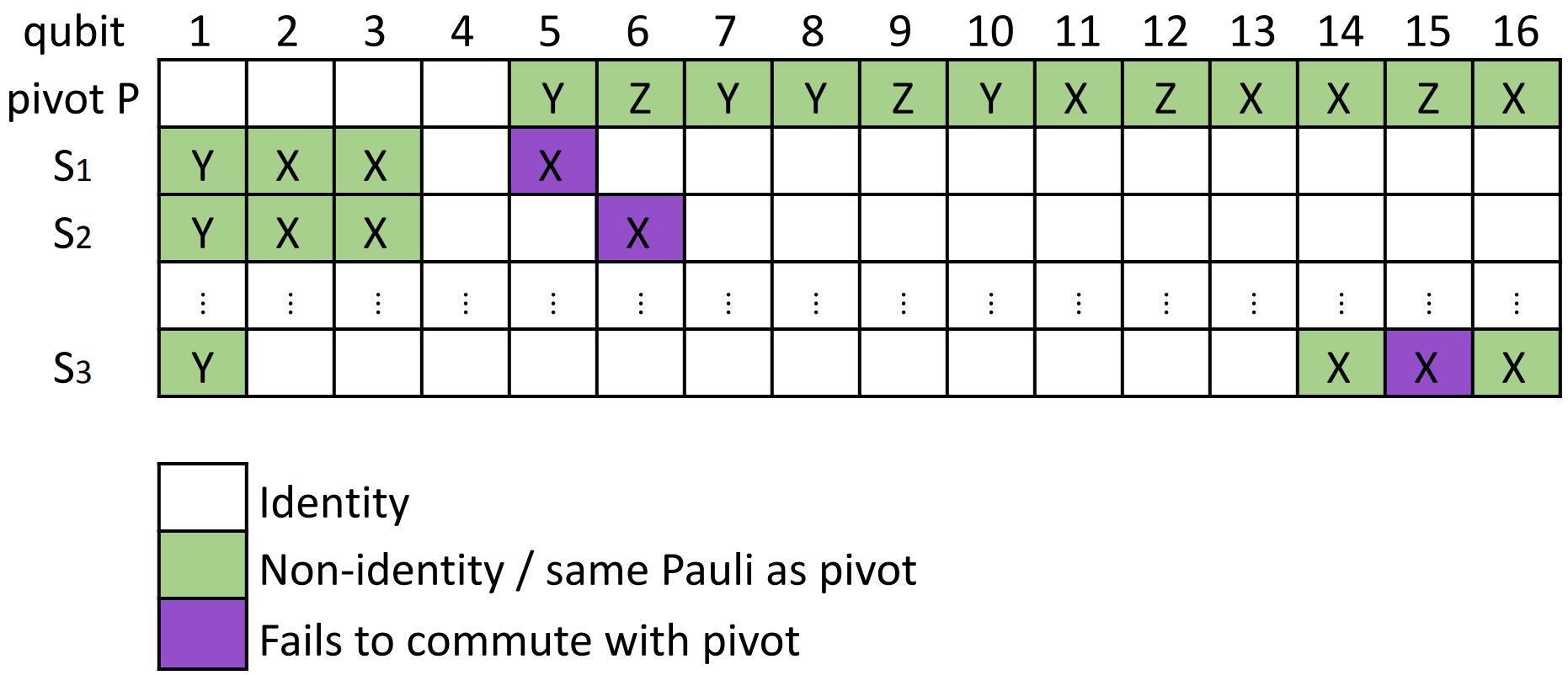
Figure 1: A subset of the $\{iY_{1}X_{j}X_{k}X_{l}\}$ set with anchor qubit 1, for an example pivot with non-identities on qubits $5-16$.

III.4 Shot-noise robustness

In subsections III.2 and III.3 we saw that it is possible to arrange the commutator of the Hamiltonian and any one pool operator into $\mathcal{O}(N^{3})$ commuting sets, and that of any one Hamiltonian term and all qubit pool operators into only $2N$ commuting sets. However, solely the number of commuting sets is not enough to determine the number of state preparations required for the task. Are there any other advantages in measuring the pool gradients term-by-term of the Hamiltonian, instead of operator-by-operator of the pool?

The error $\varepsilon$ in the estimate of the gradient of operator $A_{i}$ is given by:

$$\varepsilon^{2}=\textrm{Var}(\langle[H,A_{i}]\rangle)=\sum_{j}\lvert c_{ij}\rvert^{2}\frac{\textrm{Var}(C_{ij})}{s_{ij}},$$ (8)

where $s_{ij}$ is the number of independent samples of observable $C_{ij}$, assuming an appreciable number of terms in the sum, such that the central limit theorem can be invoked. We can then minimize $\varepsilon^{2}$ under total shot budget $S_{i}=\sum_{j}s_{ij}$ by defining the Lagrangian

$$\mathcal{L}=\sum_{j}\lvert c_{ij}\rvert^{2}\frac{\textrm{Var}(C_{ij})}{s_{ij}}+\lambda\bigg{(}S_{i}-\sum_{j}s_{ij}\bigg{)}.$$ (9)

We find

$$s_{ij}=\frac{\lvert c_{ij}\rvert\sqrt{\textrm{Var}(C_{ij})}}{\sqrt{\lambda}},$$ (10)

with

$$\frac{1}{\sqrt{\lambda}}=\frac{\sum_{k}\lvert c_{ik}\rvert\sqrt{\textrm{Var}(C_{ik})}}{\varepsilon^{2}}.$$ (11)

Setting all variances to their upper bound, we see that allotting each observable a number of samples directly proportional to its absolute weight is optimal:

$$s_{ij}=\frac{\lvert c_{ij}\rvert}{\varepsilon^{2}}\bigg{(}\sum_{k}\lvert c_{ik}\rvert\bigg{)}=\lvert c_{ij}\rvert\frac{\sqrt{S_{i}}}{\varepsilon}.$$ (12)

In particular, using Eq. (12), the fact that for nonvanishing commutators $\lvert c_{ij}\rvert=2\lvert h_{j}\rvert$, and that all pool operators can be arranged into $2N$ qubit-wise commuting sets, a worst-case shot estimate for the measurement of the expectation value of the commutator of Hamiltonian term $h_{j}H_{j}$ and all $\mathcal{O}(N^{4})$ pool operators is then

$$\bar{s}_{j}=\frac{(2N)2\lvert h_{j}\rvert\sum_{k}2\lvert h_{k}\rvert}{\varepsilon^{2}},$$ (13)

and for the entire Hamiltonian we have

$$\bar{S}_{H}=\sum_{j}\bar{s}_{j}=8N\frac{(\sum_{k}\lvert h_{k}\rvert)^{2}}{\varepsilon^{2}},$$ (14)

which implies that measuring all gradients to precision $\varepsilon$ is at worst $8N$ times as expensive as a naive VQE iteration. Realistically, about half of the terms in the sum in Eq. (12) are expected to vanish for each operator on average, and the observable variances can be estimated on the fly.

Another factor that can impact shot counts is whether or not commutators with coefficients of similar magnitude are grouped together. Consider the case where we group together Hamiltonian terms into mutually commuting sets:

$$[H,A_{i}]=\sum_{g}^{\gamma_{i}}G_{ig}=\sum_{g}^{\gamma_{i}}\sum_{j}^{\zeta_{ig}}c_{igj}C_{igj},$$ (15)

where $\gamma_{i}$ is the number of commuting sets of Hamiltonian terms, and $\zeta_{ig}$ is the number of operators in set $g$. Performing a similar minimization as before, we obtain for the expected number of state preparations for the measurement of a single gradient:

$$\bar{s}_{i}=\frac{\bigg{(}\sum_{g}^{\gamma_{i}}\sqrt{\sum_{j}^{\zeta_{ig}}\lvert c_{igj}\rvert^{2}}\bigg{)}^{2}}{\varepsilon^{2}}.$$ (16)

We see that dividing large-coefficient operators into many sets instead of combining them in few is suboptimal, from Eq. (16) and the properties of the square root. To wit:

$$\sqrt{1^{2}+2^{2}}+\sqrt{1^{2}+2^{2}}>\sqrt{1^{2}+1^{2}}+\sqrt{2^{2}+2^{2}}.$$

Thus, we should prioritize grouping large-coefficient observables together, so that shots are not squandered over-measuring unimportant terms. Although here we focused on grouping Hamiltonian terms for concreteness, the result holds more generally for various grouping strategies. In the case of our proposed strategy of grouping gradient commutators according to mutually commuting sets of pool operators, where for nonvanishing commutators $\lvert c_{ij}\rvert\propto\lvert h_{j}\rvert$, we see that this requirement is saturated: All commutators in each set have identical coefficients. We note that although we simultaneously measure commutators, each of the observables in a simultaneously measured set enters a different sum (the different operator gradients). That is, the terms in each sum are sampled from different state preparations, and our independent sampling argument, Eqs. (8)-(11), is still valid.

Not only does the proposed grouping of the gradient observables result in significantly fewer commuting sets, but it does so in a manner conscious of measurement statistics. For these reasons, we expect our Hamiltonian term-by-term partitioning to be resilient to finite sampling error and impactful in terms of shot economy, especially considering that molecular Hamiltonian coefficients typically span at least 10 orders of magnitude even for small molecules, as shown in Fig. 2. We note that the heuristic algorithms for combining Hamiltonian terms into commuting sets for energy measurement purposes in Refs. [23], and [29] prioritize combining large-coefficient observables with very promising results.

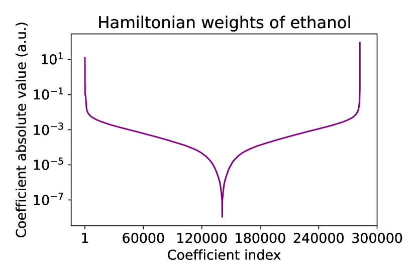
Figure 2: JW-mapped Hamiltonian coefficient absolute values for 42 spin-orbital (and qubit) ethanol in the STO-3G basis set. The left half of the curve corresponds to the positive coefficients, and the right half to the negative ones. Spanning roughly ten orders of magnitude is typical even for small molecular systems.

IV Discussion

In this work, we proposed a strategy for the efficient measurement of the gradients of certain hardware-friendly operator pools in ADAPT-VQE. It is based on the fact that the elements of any (arbitrarily large) set of mutually commuting operators share a common eigenbasis in which they can be simultaneously measured. However, the commuting commutators do not commute qubit-wise in general, which implies that their shared eigenbasis is an entangled one. Rotating it into the $Z$-basis in which the physical measurement is to be performed requires performing entangling gates. The problem of finding the unitary that implements the rotation has been studied by many others in the past [23, 24, 26, 25] and we do not attempt yet another circuit construction here. Thankfully, methods that yield circuits with at most $\mathcal{O}(\frac{N^{2}}{logN})$ entangling gates exist [30, 31], thus the significant decrease in circuit depth such pools afford is expected to far outweigh the modest increase in the total number of CNOT gates from simultaneous measurement [20, 12, 21].

In the shot-noise analysis in III.4, we assumed that we want to estimate each gradient within error $\varepsilon$, which determines the expected number of state preparations. However, determining what $\varepsilon$ should be, how a looser accuracy threshold affects the final ansatz, and how it should vary with the system size will require large-scale simulations on a variety of systems, and will be the objective of future work, along with investigating how other hyperparameters affect the performance of the algorithm.

V Conclusions

Arranging $\mathcal{O}(N^{4})$ observables in $\mathcal{O}(N)$ sets.

We introduced a method for collecting $\mathcal{O}(N^{4})$ Pauli observables of interest into $\mathcal{O}(N)$ mutually commuting sets by proving that the commutators of a set of commuting Pauli words with any other one Pauli word mutually commute. Unlike heuristic methods for grouping commuting Pauli observables that often involve generating the commutation graph, our strategy is more constructive: which terms will be grouped with which can be determined by inspection, before the list of observables of interest is even generated.

Shot-noise resistant.

We argued that our proposed strategy automatically considers shot-noise effects, since by design all observables in any single set have the same coefficients in the quantities of interest (the gradients), and each set can be allotted an optimal number of state preparations according to its importance.

$\mathcal{O}(N)$ times as expensive as naive VQE.

Using worst-case estimates, we show that the number of shots required to measure the pool gradients to error $\varepsilon$ is at most $8N$ times as expensive as naively measuring the expectation value of the Hamiltonian up to the same error.

Our approach can significantly reduce the state preparation overhead of ADAPT-VQE, and we expect it to find use in implementations of ADAPT-VQE on NISQ devices.

VI acknowledgments

We thank Yanzhu Chen for helpful discussions. S.E.E. and P.G.A. were supported by the U.S. Department of Energy, Office of Science, National Quantum Information Science Research Centers, Co-design Center for Quantum Advantage (C2QA) under contract number DE-SC0012704. E.B. and N.J.M. acknowledge support from Award No. DE-SC0019199.

References

- Peruzzo et al. [2014] A. Peruzzo, J. McClean, P. Shadbolt, M.-H. Yung, X.-Q. Zhou, P. J. Love, A. Aspuru-Guzik, and J. L. O’Brien, A variational eigenvalue solver on a photonic quantum processor, Nature Communications 5, 4213 (2014).
- Kitaev [1995] A. Y. Kitaev, Quantum measurements and the abelian stabilizer problem (1995), arXiv:quant-ph/9511026 [quant-ph] .
- Zhang et al. [2020] D.-B. Zhang, Z.-H. Yuan, and T. Yin, Variational quantum eigensolvers by variance minimization (2020), arXiv:2006.15781 [quant-ph] .
- Ryabinkin et al. [2019] I. G. Ryabinkin, S. N. Genin, and A. F. Izmaylov, Constrained variational quantum eigensolver: Quantum computer search engine in the fock space, Journal of Chemical Theory and Computation 15, 249 (2019).
- Farhi et al. [2014] E. Farhi, J. Goldstone, and S. Gutmann, A quantum approximate optimization algorithm (2014), arXiv:1411.4028 [quant-ph] .
- Kandala et al. [2017] A. Kandala, A. Mezzacapo, K. Temme, M. Takita, M. Brink, J. M. Chow, and J. M. Gambetta, Hardware-efficient variational quantum eigensolver for small molecules and quantum magnets, Nature 549, 242 (2017).
- Holmes et al. [2022] Z. Holmes, K. Sharma, M. Cerezo, and P. J. Coles, Connecting ansatz expressibility to gradient magnitudes and barren plateaus (2022), arXiv:2101.02138 [quant-ph] .
- Anand et al. [2022] A. Anand, P. Schleich, S. Alperin-Lea, P. W. K. Jensen, S. Sim, M. Díaz-Tinoco, J. S. Kottmann, M. Degroote, A. F. Izmaylov, and A. Aspuru-Guzik, A quantum computing view on unitary coupled cluster theory, Chem. Soc. Rev. 51, 1659 (2022).
- Grimsley et al. [2020] H. R. Grimsley, D. Claudino, S. E. Economou, E. Barnes, and N. J. Mayhall, Is the trotterized uccsd ansatz chemically well-defined?, Journal of Chemical Theory and Computation 16, 1 (2020).
- Grimsley et al. [2019] H. R. Grimsley, S. E. Economou, E. Barnes, and N. J. Mayhall, An adaptive variational algorithm for exact molecular simulations on a quantum computer, Nature Communications 10, 3007 (2019).
- Grimsley et al. [2023] H. R. Grimsley, G. S. Barron, E. Barnes, S. E. Economou, and N. J. Mayhall, Adaptive, problem-tailored variational quantum eigensolver mitigates rough parameter landscapes and barren plateaus, npj Quantum Information 9, 19 (2023).
- Tang et al. [2021] H. L. Tang, V. Shkolnikov, G. S. Barron, H. R. Grimsley, N. J. Mayhall, E. Barnes, and S. E. Economou, Qubit-adapt-vqe: An adaptive algorithm for constructing hardware-efficient ansätze on a quantum processor, PRX Quantum 2, 020310 (2021).
- Shkolnikov et al. [2021] V. O. Shkolnikov, N. J. Mayhall, S. E. Economou, and E. Barnes, Avoiding symmetry roadblocks and minimizing the measurement overhead of adaptive variational quantum eigensolvers (2021), arXiv:2109.05340 [quant-ph] .
- Liu et al. [2021] J. Liu, Z. Li, and J. Yang, An efficient adaptive variational quantum solver of the Schrödinger equation based on reduced density matrices, The Journal of Chemical Physics 154, 10.1063/5.0054822 (2021), 244112, https://pubs.aip.org/aip/jcp/article-pdf/doi/10.1063/5.0054822/15965352/244112_1_online.pdf .
- Nykänen et al. [2022] A. Nykänen, M. A. C. Rossi, E.-M. Borrelli, S. Maniscalco, and G. García-Pérez, Mitigating the measurement overhead of adapt-vqe with optimised informationally complete generalised measurements (2022), arXiv:2212.09719 [quant-ph] .
- Majland et al. [2023] M. Majland, P. Ettenhuber, and N. T. Zinner, Fermionic adaptive sampling theory for variational quantum eigensolvers (2023), arXiv:2303.07417 [quant-ph] .
- Warren et al. [2022] A. Warren, L. Zhu, N. J. Mayhall, E. Barnes, and S. E. Economou, Adaptive variational algorithms for quantum gibbs state preparation (2022), arXiv:2203.12757 [quant-ph] .
- Zhang et al. [2021] F. Zhang, N. Gomes, Y. Yao, P. P. Orth, and T. Iadecola, Adaptive variational quantum eigensolvers for highly excited states, Phys. Rev. B 104, 075159 (2021).
- Seeley et al. [2012] J. T. Seeley, M. J. Richard, and P. J. Love, The Bravyi-Kitaev transformation for quantum computation of electronic structure, The Journal of Chemical Physics 137, 10.1063/1.4768229 (2012), 224109, https://pubs.aip.org/aip/jcp/article-pdf/doi/10.1063/1.4768229/13999577/224109_1_online.pdf .
- Yordanov et al. [2021] Y. S. Yordanov, V. Armaos, C. H. W. Barnes, and D. R. M. Arvidsson-Shukur, Qubit-excitation-based adaptive variational quantum eigensolver, Communications Physics 4, 228 (2021).
- Anastasiou et al. [2022] P. G. Anastasiou, Y. Chen, N. J. Mayhall, E. Barnes, and S. E. Economou, Tetris-adapt-vqe: An adaptive algorithm that yields shallower, denser circuit ansätze (2022), arXiv:2209.10562 [quant-ph] .
- Verteletskyi et al. [2020] V. Verteletskyi, T.-C. Yen, and A. F. Izmaylov, Measurement optimization in the variational quantum eigensolver using a minimum clique cover, The Journal of Chemical Physics 152, 124114 (2020).
- Crawford et al. [2021] O. Crawford, B. v. Straaten, D. Wang, T. Parks, E. Campbell, and S. Brierley, Efficient quantum measurement of Pauli operators in the presence of finite sampling error, Quantum 5, 385 (2021).
- Gokhale et al. [2019] P. Gokhale, O. Angiuli, Y. Ding, K. Gui, T. Tomesh, M. Suchara, M. Martonosi, and F. T. Chong, Minimizing state preparations in variational quantum eigensolver by partitioning into commuting families (2019), arXiv:1907.13623 [quant-ph] .
- Yen et al. [2020] T.-C. Yen, V. Verteletskyi, and A. F. Izmaylov, Measuring all compatible operators in one series of single-qubit measurements using unitary transformations, Journal of Chemical Theory and Computation 16, 2400 (2020), pMID: 32150412, https://doi.org/10.1021/acs.jctc.0c00008 .
- van den Berg and Temme [2020] E. van den Berg and K. Temme, Circuit optimization of Hamiltonian simulation by simultaneous diagonalization of Pauli clusters, Quantum 4, 322 (2020).
- Gokhale et al. [2020] P. Gokhale, O. Angiuli, Y. Ding, K. Gui, T. Tomesh, M. Suchara, M. Martonosi, and F. T. Chong, measurement cost for variational quantum eigensolver on molecular hamiltonians, IEEE Transactions on Quantum Engineering 1, 1 (2020).
- Bailey and Stevens [2010] R. F. Bailey and B. Stevens, Hamiltonian decompositions of complete k-uniform hypergraphs, Discrete Mathematics 310, 3088 (2010), combinatorics 2008.
- Choi et al. [2022] S. Choi, T.-C. Yen, and A. F. Izmaylov, Improving quantum measurements by introducing “ghost” pauli products, Journal of Chemical Theory and Computation 18, 7394 (2022), pMID: 36332111, https://doi.org/10.1021/acs.jctc.2c00837 .
- Van den Nest et al. [2004] M. Van den Nest, J. Dehaene, and B. De Moor, Graphical description of the action of local clifford transformations on graph states, Phys. Rev. A 69, 022316 (2004).
- Patel et al. [2008] K. N. Patel, I. L. Markov, and J. P. Hayes, Optimal synthesis of linear reversible circuits, Quantum Info. Comput. 8, 282–294 (2008).