The emergence of relaxation-oscillator convection on Earth and Titan

Abstract

In relaxation-oscillator (RO) climate states, short-lived convective storms with torrential rainfall form and dissipate at regular, periodic intervals. RO states have been demonstrated in two- and three-dimensional simulations of radiative-convective equilibrium (RCE), and it has been argued that the existence of the RO state requires explicitly resolving moist convective processes. However, the exact nature and emergence mechanism of the RO state have yet to be determined. Here, we show that (1) RO states exist in single-column-model simulations of RCE with parameterized convection, and (2) the RO state can be understood as one that has no steady-state solutions of an analytical model of RCE. As with model simulations with resolved convection, these simpler, one-dimensional models of RCE clearly demonstrate RO states emerge at high surface temperatures and/or very moist atmospheres. Emergence occurs when atmospheric instability quantified by the convective available potential energy can no longer support the latent heat release of deep, entraining convective plumes. The proposed mechanism for RO emergence is general to all moist planetary atmospheres, is agnostic of the condensing component, and naturally leads to an understanding of Titan’s bursty methane weather.

1 Introduction

Earth’s tropics are characterized by a steady balance between heating by moist convection and radiative cooling, which is referred to as quasi-equilibrium (QE) convection. QE states exhibit continuous, deep convection and small, random fluctuations in clouds and precipitation about the mean. A new mode of convection with quasi-periodic oscillations was recently discovered for high surface temperatures in three-dimensional, cloud-resolving model simulations of radiative-convective equilibrium (3D-RCE; Seeley & Wordsworth, 2021a, henceforth SW21). In this new relaxation-oscillator (RO) mode of convection, storms erupt at regular intervals with vigorous, short-lived rainfall, separated by dry, cloud-free spells. Although the RO state is not a feature of the modern climate, significant time-variation in convective storms have been observed or simulated in a variety of planetary environments: from Jupiter (Sugiyama et al., 2014) and Saturn (Li & Ingersoll, 2015; Fischer et al., 2011) to Titan (Schaller et al., 2009; Turtle et al., 2011) and the hothouse Earth (SW21).

SW21 propose that the physical ingredients required for RO states are (i) realistic radiation, (ii) clouds, (iii) convection, and (iv) large-scale condensation and re-evaporation; they further speculate that RO states require model simulations with resolved convection, i.e., a model of 3D-RCE. These four ingredients, however, are not unique to 3D-RCE – all of them can be parameterized in simpler models of RCE. In this paper, we demonstrate the existence of RO states in a single-column model of RCE, i.e., 1D-RCE. We then develop a hypothesis for the emergence of RO states by exploring the limits of an even simpler, QE model of RCE, and test our hypothesis against our 1D-RCE simulations and the 3D-RCE simulations of SW21. To illustrate the flexibility of our approach, we test it against a completely different moist-convective system: methane on Titan.

2 Methods

We use a version of the ECHAM6 GCM in single-column mode that has been modified to allow water vapor to comprise a significant fraction of the atmospheric mass (Popp et al., 2015, henceforth P15) and the SVP of water to be multiplicatively altered (Spaulding-Astudillo & Mitchell, 2023). The single-column model has separate schemes for radiation, convection, and clouds. Shortwave and longwave radiation is resolved into 14 and 16 spectral bands by the Rapid Radiative Transfer Model for General Circulation Models (RRTMG - Iacono et al., 2008). All phases of water are prognostic and accounted for in the radiation calculation. As in P15, we use an exponential extrapolation of all molecular absorption coefficients in the longwave and the H2O self-broadened absorption coefficients in the shortwave for temperatures above which no data in the original model exists. The effect of pressure broadening by water vapor is neglected. Convection is represented by a bulk-plume scheme (Tiedtke, 1989; Giorgetta et al., 2013) that parameterizes turbulent entrainment and detrainment of air between updrafts, downdrafts, and the environment. Clouds are formed by a large-scale condensation and re-evaporation scheme (Sundqvist et al., 1989) as a function of the relative humidity of the environment.

In our minimal-recipe experiment, the insolation is set 10% higher than the present-day value and is temporally fixed (no diurnal or seasonal cycle). We set the column latitude to 38^∘N, where the globally-averaged insolation is the same as the local value. Clouds are the only source of time-varying planetary albedo. The atmosphere is composed only of nitrogen, oxygen, and water vapor. We use a time step of 60 s and run the simulations for approximately 200 years. The sea surface temperature (SST or $T_{s}$) of a 1 m mixed-layer ocean with an albedo of 0.07 is fixed at every time step through the use of an artificial surface heat sink. We use fixed $T_{s}$ and vary it in 1-5 K increments from 290 to 370 K.

3 Results

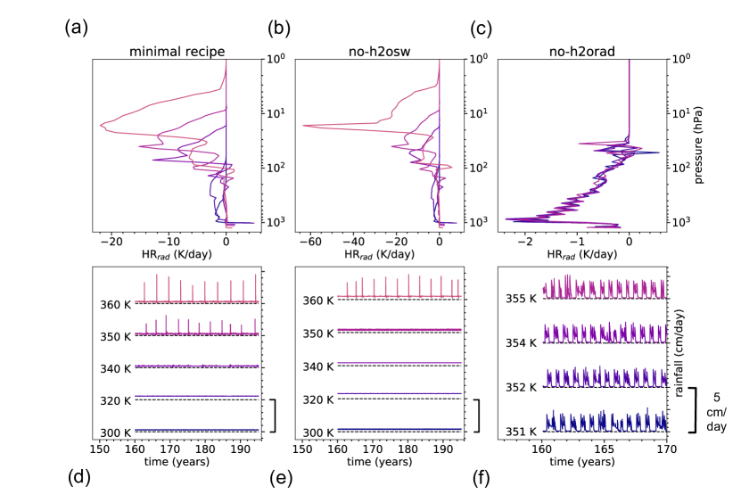
Figure 1: Displays (left to right) the minimal recipe, no-h2osw, and no-h2orad single column experiments with fixed SSTs between 300-360 K. The top row is net radiative temperature tendency in K/day. The bottom row is a time-series of rainfall rates in cm/day over a 30 year period. Rainfall rates at each SST are vertically offset by 5 cm/day and a zero rainfall contour is given for reference as a dashed black line.

3.1 Description of RO states

Figure 1d clearly shows that our single column, minimal-recipe simulations transition into RO states at a surface temperature around $T_{s}=350$ K. At cooler temperatures, precipitation is steady and continuous and hovers around a mean value of 2-6 mm/day; these simulations are in the QE regime. RO states exhibit large bursts of precipitation with intensities up to 5 cm/day that repeat every $O(100)$-$O(1000)$ days and that are relatively short-lived (10-30 days). Consistent with 2D (Sugiyama et al., 2014) and 3D (SW21) simulations of oscillatory climate states, 1D-RCE RO states cycle through 3 phases: a rapid convective phase (RCP), a slow cooling phase (SCP), and a triggering phase (TP).

In the RCP, deep convection rapidly heats and moistens the atmosphere above the boundary layer at $O(1)$-$O(10)$ K/day (Figure 2b). The storm generates a spike in rainfall resembling a delta function that is 10-20 times stronger than the mean background rate (Figure 2d). Strong warming disrupts cloud formation by reducing the column relative humidity, contributing to a sharp drop in vertically-integrated cloud water of 1-2 orders of magnitude (Figure 2a). Low-level temperature inversions in our warmest simulations are a clear source of convective inhibition that form during the RCP and are slowly eroded during the subsequent SCP; such inversions are common to the so-called moist greenhouse state (Wolf & Toon, 2015; Popp et al., 2015).

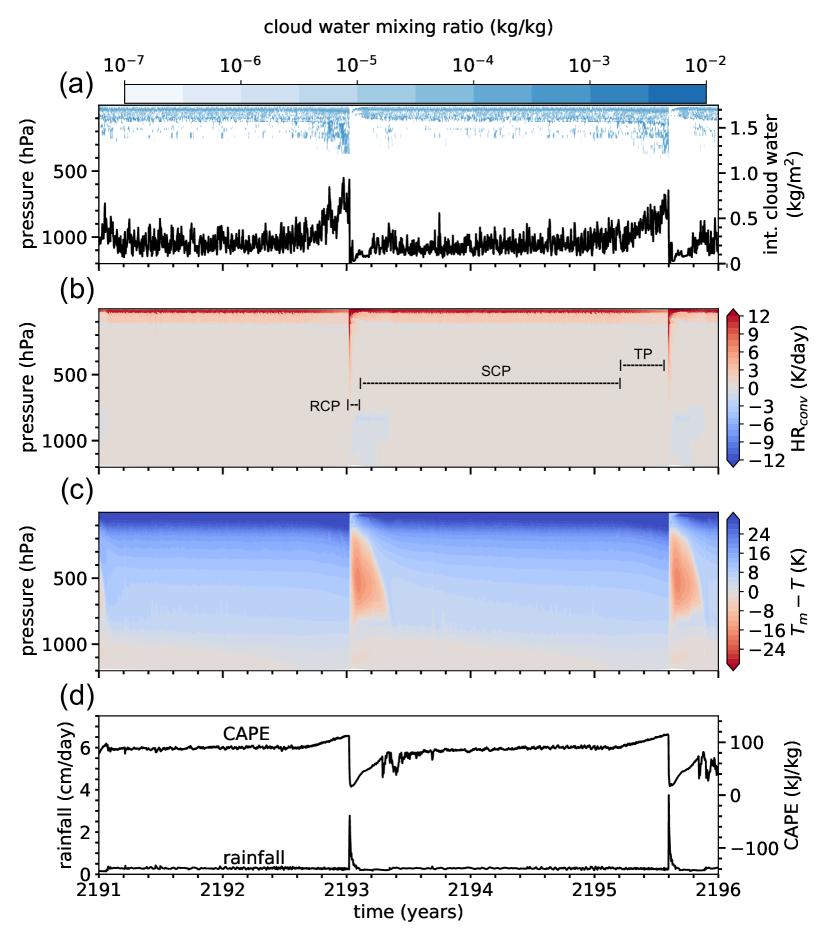
Figure 2: Time series of the minimal-recipe experiment over 5 years at $T_{s}=355$ K. Depicts (a) cloud water mixing ratio in color and vertically-integrated cloud water in black. (b) Temperature tendency from the convection scheme in K/day. (c) Difference in temperature between a parcel lifted from the surface along the moist pseudo-adiabat and the environment. This is a proxy for the atmospheric instability. (d) Rainfall rate and convective available potential energy (CAPE).

During the SCP, the atmosphere cools radiatively from its upper layers. The lower layers are water-dominated and thus are unable to cool directly to space because of their high infrared opacity. Top-of-atmosphere radiative cooling is communicated to the lower layers through the re-evaporation of precipitation; re-evaporation destablizes the atmosphere from the top down, building CAPE in the process (Figure 2c,d). The increase in CAPE is evident in a time series of the difference in temperature between the surface-defined moist pseudo-adiabat and the environment (Figure 2c). Total cloud cover steadily increases over the SCP (Figure 2a).

The TP begins when the troposphere is everywhere unstable with respect to surface-based, pseudo-adiabatic moist convection (Figure 2c). A striking feature of the TP is the rapid descent of the cloud base (Figure 2a), which has been observed in other numerical studies of oscillatory climate states (SW21, Sugiyama et al., 2014). Vertically-integrated cloud water quadruples during this period (Figure 2a), which could be related to the troposphere nearing saturation. Eventually, the built-up CAPE is released (Figure 2d) and the cycle repeats from the RCP.

The inhibitive cap that exists during the SCP is slowly eroded away by the TP (Figure 2c). Paradoxically, CAPE continues to grow during the TP with no apparent convective inhibition mechanism (Figure 2d). In fact, the TP typically represents over 25% of the quiescent period. This means that there is a significant delay between when the troposphere becomes globally unstable and when the next storm begins. This apparent paradox suggests that we have thus far overlooked an emergent constraint on deep convection, which we will return to in Section 3.3.

3.2 RO states occur in the absence of lower-tropospheric radiative heating

SW21 hypothesize that lower-tropospheric radiative heating (LTRH) that emerges in hot climate states is essential for the emergence of RO convection; LTRH is a consequence of strong shortwave absorption by water vapor. By enforcing LTRH in fixed SST 3D-CRM simulations, SW21 observed that RO states emerged at SSTs over 20 K less than their default experiment.

To test the LTRH hypothesis, we ran two separate mechanism-denial experiments in which we zero out the contribution of water vapor in the SW radiative calculation (“no-h2osw” experiment) and one in which it is zeroed out in the SW and LW radiative calculation (“no-h2orad” experiment). The lower troposphere remains opaque to infrared radiation in the no-h2osw experiment and consequently net cooling rates there remain close to zero (Figure 1b). In contrast, the whole troposphere radiatively cools in the no-h2orad experiment (Figure 1c). In both the no-h2osw and no-h2orad experiments, we found that RO-like states still occur (Figures 1e,f). From these mechanism-denial experiments, we conclude that the radiative effects of water vapor influence RO states, but they do not tell the whole story. We suspect that a previously-unrecognized constraint on convection produces the RO phenomenon over warm SSTs, which we now detail.

3.3 The mechanism for the emergence of RO states

The QE state is characterized by a steady balance between the generation of CAPE by radiation and its destruction by convection. The RO state is clearly not steady, however we posit that exploring the conditions in which a steady, QE state is valid can illuminate the mechanisms that lead to the transition from QE to RO convection. We carry this out quantitatively in Section 3.4, but first consider heuristically how the dynamics of RO convection would differ from the QE state. Essential to the QE state is the ability of radiative cooling to keep pace with the more rapid convective heating. In warm and/or humid conditions, however, the fast convective process releases an amount of latent energy that the slower radiation cannot keep pace with. The sudden release of this heat, $\langle r\rangle$, in convection would naturally stabilize the atmosphere and shut off convection until radiation can restore buoyancy. CAPE would necessarily be time-dependent, undergoing large oscillations bounded above by $\langle r\rangle$. In this picture, the RO state emerges when $\langle r\rangle$ exceeds the value of CAPE that would be present in the QE regime. Thus, a predictive model of RO emergence requires a plausible model of quasi-steady RCE.

Just such a steady-state model of QE convection has gained traction in recent years (Singh & O’Gorman, 2013; Romps, 2014, 2016; Seeley & Wordsworth, 2023). Romps (2016, henceforth R16) conceives of a saturated, convective plume interacting with a sub-saturated environment with which it has zero buoyancy – the so-called “zero-buoyancy model” (ZBM) – a condition that is supported by observations in the tropics and in cloud-resolving models simulations (see Section 3.4 for a derivation of the ZBM.). The ZBM predicts the steady value of CAPE that would be present in QE for a given surface temperature and a set of convective parameters. It’s important to note that the CAPE predicted by the ZBM represents a steady-state storage of buoyancy, not the rate of CAPE generation and destruction by radiation and convection. Furthermore, the ZBM predicts a maximum in CAPE at intermediate, warm surface temperatures, which are explored quantitatively in the following sections. Concurrently, increasing the SST would naturally increase water vapor, and we will show that the latent heat release by convection in the ZBM, $\langle r\rangle$, increases monotonically with surface temperature. Thus, $\langle r\rangle$ inevitably exceeds the steady value of CAPE above a certain SST; above this SST, the QE state is no longer viable. Our hypothesis is that the RO state is preferred in this SST regime.

In what follows, we calculate CAPE and $\langle r\rangle$ of the ZBM as a function of SST, and convective and thermodynamic parameters. We then test our hypothesis for the emergence of RO states by seeking the answers to the questions: (1) Under what conditions does $\langle r\rangle$ exceed CAPE in the ZBM?; and (2) Is the point of divergence between $\langle r\rangle$ and CAPE predictive of the emergence of RO states in simulations?

3.4 CAPE and $\langle r\rangle$ in an analytical model of an atmosphere in RCE

Parameter	Definition	Earth-like	Titan-like
$c_{p,d}$	Specific heat of dry air at constant pressure (Jkg-1K-1)	1004	1040
$R_{d}$	Specific gas constant of dry air (Jkg-1K-1)	287	290
$R_{v}$	Specific gas constant of the condensable (Jkg-1K-1)	462	518
$L$	Latent heat of vaporization of the condensable (Jkg-1)	$2.26\times 10^{6}$	$5.5\times 10^{5}$
$g$	Gravitational acceleration (ms-2)	9.81	1.35
$T_{trp}$	Tropopause temperature (K)	200	70
$p_{s,d}$	Partial pressure of dry air at the surface (Pa)	$10^{5}$	$1.42\times 10^{5}$

Table 1: Parameters used to evaluate the analytical QE model at Earth-like and Titan-like conditions. These are not necessarily the values used by ECHAM6 (Stevens et al., 2013) or the Titan Atmospheric Model (TAM - Lora et al., 2015).

The system of equations for the analytical QE model of RCE derived are presented below, to which we have contributed two innovations. First, we introduce an artificial multiplier on the saturation vapor pressure (SVP) of water, $\xi$, following Spaulding-Astudillo & Mitchell (2023) and McKinney et al. (2022).

$$e^{*}_{\xi}=\xi e^{*}$$ (1)

where $e^{*}_{\xi}$ and $e^{*}$ are the modified and true SVP of water, respectively. Moisture variables with a subscript of $\xi$ should be understood to have an implicit $\xi$-dependence. Second, and most importantly, we extend the analytical model to solve for $\langle r\rangle$. We refer the reader to Appendix A for the extended derivation.

Under the assumption that the convective mass flux, the relative humidity of the environment, and precipitation efficiency (PE - defined as the fraction of condensates generated in updrafts at each height that are not re-evaporated) are constant with height, the system of equations for an RCE atmosphere are

$$q^{*}_{\xi} = \frac{R_{a}}{R_{v}}\frac{e^{*}_{\xi}}{p},$$ (2)

$$-\gamma = \frac{g}{R_{a}T}-\frac{L\Gamma}{R_{v}T^{2}},$$ (3)

$$\varepsilon = \frac{\gamma a}{\textrm{PE}},$$ (4)

RH $$= \frac{1+a-\textrm{PE}}{1+a},$$ (5)

$$c_{z} = \frac{\gamma q^{*}_{\xi}}{1+a},\hskip 3.61371pt\textrm{and}$$ (6)

$$\Gamma = \frac{g}{c_{p,d}}\Big{[}\frac{1+a+q^{*}_{\xi}L/(R_{a}T)}{1+a+q^{*}_{\xi}L^{2}/(c_{p}R_{v}T^{2})}\Big{]}.$$ (7)

The thermodynamic constants and their units and values are given in Table 1 and are assumed to be constant with height. $q^{*}_{\xi}$ is saturation specific humidity ($kg_{h2o}$kg^-1), $\gamma$ is the water vapor lapse rate (kg_h2okg^-1m^-1), $\varepsilon$ is the fractional convective entrainment (m^-1), RH is the relative humidity, $c_{z}$ is the specific condensation per unit distance traveled by an entraining plume (kg_h2okg^-1m^-1), and $\Gamma$ is the temperature lapse rate (Km^-1). PE and $a$ are prescribed constants; by Equation 4, their ratio is a constant equal to $\gamma/\varepsilon$ ($\gamma$ and $\varepsilon$ both increase with height but do so in lock-step). $a$ controls the dilution of convective plumes by environmental air (for an extended discussion, see Seeley & Wordsworth, 2023). For undiluted convection ($a=0$) in a real atmosphere ($\xi=1$), $\Gamma$ equals the moist pseudo-adiabatic lapse rate, $\Gamma_{m}$. As $a$ increases, the tighter coupling between the plume and the environment forces $\Gamma$ apart from $\Gamma_{m}$, permitting more convective instability in steady-state. We calculate the instability in steady-state as

$$\textrm{CAPE}=\int_{z_{s}}^{z_{trp}}g\frac{T^{\prime}-T}{T}dz,$$ (8)

where $T$ is the environmental temperature and $T^{\prime}$ is the temperature of a parcel lifted moist pseudo-adiabatically from the surface ($z_{s}$) to the tropopause ($z_{trp}$). The net release of latent energy per unit mass of an entraining plume traveling from the surface to the tropopause is

$$\langle r\rangle=L\frac{\textrm{PE}}{1+a}\Big{(}q^{*}_{\xi}(T_{s})-q^{*}_{\xi}(T_{trp})\Big{)}.$$ (9)

Equation 9 clearly relates the moisture lost by a saturated plume during ascent, $q^{*}_{\xi}(T_{s})-q^{*}_{\xi}(T_{trp})$, to the details of turbulent mixing and evaporative microphysics, $\textrm{PE}/(1+a)$, and to the latent heat, $L$. Since $\langle r\rangle$ and CAPE share the same physical units (J kg^-1), we are equipped mathematically to compare their magnitudes in steady-state as a function of SST in Section 3.5. The sensitivity of CAPE and $\langle r\rangle$ to $\xi$ allow us to test the mechanism for the emergence of RO states in Section 3.6.

3.5 The physical relationship between CAPE and $\langle r\rangle$

How are $\langle r\rangle$ and CAPE related physically? CAPE (Equation 8) is proportional to the height-integrated temperature difference between an undiluted lifted parcel and its environment, $\Delta T$, which can be approximated following R16 as

$$\textrm{CAPE}\propto\int_{z_{s}}^{z_{trp}}\Delta Tdz\approx\int_{z_{s}}^{z_{trp}}\frac{\Delta h_{\xi}^{*}}{\beta}dz.$$ (10)

$\Delta h_{\xi}^{*}$ is the saturated moist static energy (MSE) difference between the two air masses at height $z$ and $\beta=c_{p,d}+L^{2}q^{*}_{\xi}/(R_{v}T^{2})$ is the atmospheric heat capacity at height $z$. $\beta^{-1}$ gives the fraction of the saturated MSE difference that is expressed as a temperature anomaly or, equivalently, as CAPE. $\Delta h_{\xi}^{*}$ can also be expressed as (R16)

$$\Delta h^{*}_{\xi}=\frac{a}{1+a}L\Big{(}q^{*}_{\xi}(z_{s})-q^{*}_{\xi}(z)\Big{)}.$$ (11)

This allows us to rewrite $\langle r\rangle$ (Equation 9) as

$$\langle r\rangle=\frac{\textrm{PE}}{a}\Delta h_{\xi}^{*}(z_{trp}).$$ (12)

The ratio $\textrm{PE}/a=\gamma/\varepsilon$ (a constant in this restricted model of RCE, but in practice varies in real atmospheres) is the fraction of the saturated MSE at a given height that is expressed as $\langle r\rangle$. Given Equations 10 and 12, it’s clear that CAPE and $\langle r\rangle$ are both closely related to $\Delta h_{\xi}^{*}$. At lower SSTs, both $\langle r\rangle$ and CAPE grow in proportion to $q_{\xi}^{*}$ by Equation 11. Unlike $\langle r\rangle$, however, CAPE peaks at intermediate SSTs because of its dependence on $1/\beta$, which decreases rapidly at high SSTs. CAPE begins this decrease with increasing SSTs where $\beta>2c_{p,d}$ at the tropopause (see Figure 9 from R16), or in other words where the effective heat capacity of the entire troposphere becomes moisture-dominated. Thus, the magnitude of CAPE is set by a competition between the increase in $\Delta h_{\xi}^{*}$ and decrease in $1/\beta$, the latter of which wins out in the warmest (Figure 3) and/or wettest (Figure 4) environments. Further increasing the SST beyond the peak in CAPE result in a smaller fraction of $\Delta h_{\xi}^{*}$ that is expressed as CAPE through $\Delta T$ and a constant fraction and therefore growing amount of $\Delta h_{\xi}^{*}$ that is expressed as $\langle r\rangle$. Any SSTs for which $\langle r\rangle>\textrm{CAPE}$ violate the steady-state assumption of the RCE model, inevitably pushing convection from the QE state into the RO state.

3.6 Testing the emergence mechanism for RO states

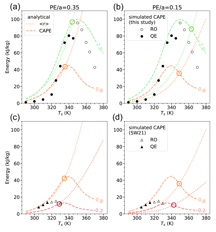
Figure 3: Analytical CAPE (dashed) and $\langle r\rangle$ (dotted) for an Earth-like atmosphere with PE/a ratios of (a,c) 0.35 and (b,d) 0.15. Values of $a$ ranging between 0.2 and 2.8 are denoted by in-line labels and specific line colors. Like-colored open circles are placed at the theoretical location of each QE-to-RO transition, i.e., where the dotted and dashed lines with the same value (color) of $a$ intersect. CAPE from our minimal-recipe simulations is given as black circles and CAPE from Seeley & Wordsworth (2021b) is given as black triangles. Filled circles/triangles denote QE states and open circles/triangles denote RO states.

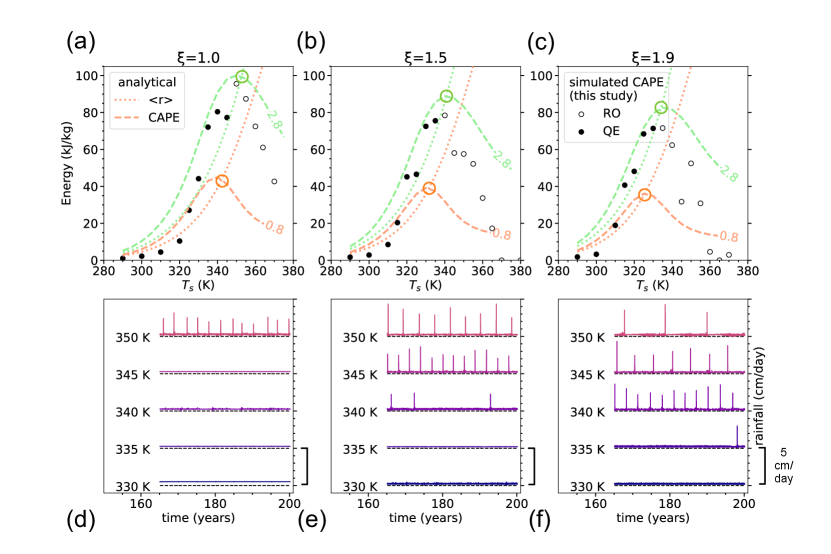
Figure 4: Sensitivity experiments for an Earth-like atmosphere with (a,d) $\xi=1$, (b,e) $\xi=1.5$, and (c,f) $\xi=1.9$. (a-c) Analytical CAPE (dashed) and $\langle r\rangle$ (dotted) with PE=25%. Values of $a$ ranging between 0.2 and 2.8 are denoted by in-line labels and specific line colors. Like-colored open circles are placed at the theoretical location of each QE-to-RO transition, i.e., where the dotted and dashed lines with the same value (color) of $a$ intersect. CAPE from our minimal-recipe simulations is given as black circles. Filled circles denote QE states and open circles denote RO states. (d-f) Time series of rainfall rate over a 30 year period for minimal-recipe simulations with fixed SSTs between 330-350 K. The profile from each simulation is vertically offset by 5 cm/day and a zero rainfall contour is given for reference as a dashed black line.

We first specify two convective parameters which are assumed to be constant with height: PE and $a$. PE is the fraction of condensates generated in ascending plumes that are re-evaporated in the environment. $a$ quantifies the dilution of plumes by the environment, and represents the combined effect of entrainment and re-evaporation. The quantity $\textrm{PE}/a$ may be estimated as the water vapor lapse rate, $\gamma$, divided by the convective entrainment rate, $\varepsilon$, over the troposphere. Typical values of $\varepsilon$ and $\gamma^{-1}$ in Earth’s atmosphere at 300 K are $0.5-2\times 10^{-3}$ km^-1 (Romps, 2010) and 2-8 km (R16). Taking intermediate values gives an expected value for Earth of $\textrm{PE}/a=0.25$. Figure 3 shows theoretical profiles of CAPE and $\langle r\rangle$ evaluated with the thermodynamic constants in Table 1 in the neighborhood of this $\textrm{PE}/a$ ratio. Reducing $\textrm{PE}/a$ (between columns in Figure 3) has no effect on CAPE because CAPE is a function of $a$ only.

Regardless of the convective parameter values, $\langle r\rangle$ inevitably exceeds CAPE at some SST, as shown in Section 3.5. The SST at which this first occurs can be found by identifying the intersection of the analytical profiles of CAPE (dashed lines) and $\langle r\rangle$ (dotted lines) that possess the same value (color) of $a$ (Figure 3). The CAPE from our 1D-RCE simulations is in rough agreement with the theoretical curve denoted by $a=2$ (not plotted); for the range of $\textrm{PE}/a$, the intersection between CAPE and $\langle r\rangle$ occurs at SSTs $\sim 340-350$K (Figures 3a,b), which is also the SSTs where our simulations transition to the RO state (Figure 1d).

Extrapolating to other values of PE and $a$, the analytical model of steady-state convection predicts that decreasing $a$ and/or increasing PE shifts the intersection of CAPE and $\langle r\rangle$ to lower SSTs. Decreasing $a$ brings the analytical model into closer agreement with the results of SW21 (Figures 3c,d), which had SSTs at emergence of RO states closer to 320K. A consistent interpretation is that the 3D-RCE simulations of SW21 have a lower value of $a$ and/or higher value of PE than our 1D-RCE simulations. Differences between models in, for instance, the tuning of evaporative microphysics would naturally lead to an offset with respect to the SST at which RO states emerge.

The convection and re-evaporation schemes in our 1D-RCE model were not designed in a way that facilitates sensitivity tests using $a$ or PE as independent control parameters. However, we introduce a multiplier on SVP (Spaulding-Astudillo & Mitchell, 2023) into the analytical model of R16 whereby increasing it accomplishes a similar effect as to increasing $\textrm{PE}/a$ (this part increases $\langle r\rangle$ – see Section 3.5) while simultaneously decreasing $a$ (this part decreases CAPE). The emergence temperature in our 1D-RCE simulations dropped from 350 K to 335 K for a doubling of $\xi$, in agreement with our analytical model (Figures 4a-c). Furthermore, the analytical QE model predicts a decrease in the peak CAPE and a shift to lower SSTs with increasing $\xi$, which is borne out by our numerical experiments (Figures 4a-c). As in the other parameter regime (Figure 3), $\langle r\rangle$ and CAPE both grow quasi-exponentially with increasing SSTs to a peak in CAPE, beyond which the latter falls off with increasing SSTs while $\langle r\rangle$ continues to grow. Thus, we find that our hypothesis that the emergence of RO states is sensitive to moisture concentration is supported by the quantitative agreement between the analytical model prediction and numerical sensitivity experiments with varying SVP.

4 Discussion

We conclude that relaxation-oscillator (RO) convection is an emergent phenomenon in sufficiently warm and/or wet atmospheres. We obtained this result in a 1D-RCE model with parameterized convection that clearly reproduces the RO states that develop in 3D-RCE with resolved convection (SW21). Switching off the radiative effects of water vapor in 1D-RCE, we demonstrated that lower-tropospheric radiative heating is non-essential for RO convection. Since RO states are clearly non-steady, we hypothesized that RO states should emerge in conditions where the energetics of moist convection violate steady-state quasi-equilibrium (QE). QE is violated when the latent energy released by deep, entraining convection ($\langle r\rangle$) exceeds the convective available potential energy (CAPE) in steady-state. The RO mode of convection is preferred in these conditions in two ways. First, the surface temperature of RO emergence in 1D- and 3D-RCE agrees with the prediction from an analytical QE model evaluated with Earth-like convective parameters. Second, doubling the SVP of water at all temperatures ($\xi=2$) causes the surface temperature of emergence to decrease by 10-15 K in 1D-RCE, once again in agreement with the analytical prediction. The agreement is reassuring, as the bulk plume equations of convection of the analytical model are based on the parameterized convection scheme in our 1D-RCE model (see Methods). The consistency of the QE-to-RO convective regime transition across the modeling hierarchy explored here lends confidence to the robustness of this transition, and the insights gained from the simpler end of the modeling hierarchy developed here illustrates their power in the exploration of the sensitivity of these states to model parameters rooted in the physical world.

We note three reported commonalities between this and other studies of oscillatory radiative-convective states in both nitrogen- and hydrogen-rich atmospheres (e.g., SW21 and Sugiyama et al., 2014): (1) the slow erosion of a stable layer during the quiescent, storm-free period (SCP) followed by the descent of the cloud base (TP), (2) a significant temporal delay between the development of global tropospheric instability (TP) and the start of the next storm (RCP), and (3) an abrupt end to each storm when CAPE drops to zero (e.g., Figure 2d). We speculate that (2) and (3) could be explained by the requirement that CAPE build well above its expected steady-state value in order to accommodate the energy released by deep convection, as represented by $\langle r\rangle$. CAPE builds in time until it reaches values near $\langle r\rangle$, at which point all of the CAPE would be converted to heat in a short period of time, and the CAPE would begin building again by the slower process of radiative cooling. In this sense and in analogy to an RO electric circuit, radiative cooling and virga act as the voltage source, CAPE acts as the capacitor, and $\langle r\rangle$ acts as the threshold device.

There are at least two major differences between simulated RO states in our single column model and those in a 3D-CRM (SW21). The first difference is the SST above which RO states emerge, which is 30 K higher in this study than in SW21. In Section 3.6, we hypothesized this difference is related to different model assumptions about the details of convective mixing and re-evaporation, and we demonstrated a case in which altering the SVP of water gave rise to 10-15 K differences in the SST of RO onset. The second difference is the recurrence interval (RI), or the typical duration of the quiescent period. In SW21, the RI is $O(1)$ day and here $O(100)$-$O(1000)$ days. Of course, the time-dependent behavior of the RO state is beyond the scope of our steady-state theory, and the simulations are telling us that the RO regime is where convection is non-steady. We might better understand the relevant time scales, peak precipitation rates, etc. of the RO state by deriving linearized non-steady forms of the bulk-plume equations that appear in Section 3.4. These timescales, for instance, could then be compared to historical observations of giant storms on solar system planets. We leave this to future work.

In our derivation of the R16 model, we made several approximations and omissions (virtual effects being one of them) that introduce error in the limit of a moisture-dominated atmosphere. Revisiting these assumptions is a necessary next step, but is beyond the scope of this paper. Consistent with a recent study (Seeley & Wordsworth, 2023), the CAPE in our numerical simulations peaks at intermediate SSTs and falls to zero in the limits of a dry atmosphere or a moisture-dominated atmosphere. In Section 3.5, we discussed the “shape of CAPE”, i.e., how the magnitude of CAPE changes with SST in the steady-state model (R16). Including virtual effects in Equation 8 causes the magnitude of the CAPE from our simulations to increase at each $T_{s}$ (up to 50% at the peak), but does not significantly change the location of the peak nor the qualitative shape of CAPE vs. SST (not shown). We chose to omit virtual effects in the CAPE calculation because it allows us to directly compare our simulations to the analytical QE model.

5 RO convection on Titan

While present-day Earth does not exhibit RO behavior, it is clear that episodic storms of potentially great magnitude occur on present-day Titan (Schneider et al., 2012; Turtle et al., 2011; Faulk et al., 2017; Rafkin et al., 2022; Charnay et al., 2015; Mitchell & Lora, 2016). A plausible assumption is that the physics of moist convection should be similar on Titan and Earth. Given what we know about Titan, is RO-like moist (methane) convection predicted by the analytical theory at Titan-like conditions (see Table 1)? Our theory of RO emergence requires the input parameters of our analytical model, which are difficult to estimate from the data, but insights can be gained by making reasonable estimates. We estimate the mean methane scale height from Equation 3, $\gamma^{-1}\approx 20$ km, which aligns with an earlier estimate (Lemmon et al., 2002). Following Griffith et al. (2000), we use an entrainment rate of $\varepsilon=0.1$ km^-1. Centering our search around the expected $\textrm{PE}/a$ value of 0.5, we look for analytical solutions for RCE on Titan (Figure 5). In most cases, the analytical model predicts that $\textrm{CAPE}<\langle r\rangle$ at the present day surface temperature of Titan of 90-95 K. Only present-day scenarios with $\textrm{PE}/a\leq 0.1$ favor QE over RO convection. These scenarios, however, imply a mean tropospheric relative humidity (RH) greater than 90%, which is inconsistent with observations of episodic rainstorms over Titan’s arid low latitudes (Turtle et al., 2011), the frequency of Titan’s storms (Battalio et al., 2022), and the paucity of global cloud cover (Griffith et al., 2000). Our theory thus predicts a transition from RO to QE behavior on Titan at high RH; just such a transition from discrete to continuous precipitation was found in 3D simulations of Titan by raising the prescribed background RH above 85% (Battalio et al., 2022).

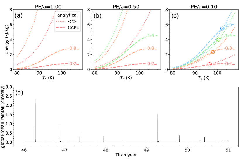
Figure 5: Analytical CAPE (dashed) and $\langle r\rangle$ (dotted) for a Titan-like atmosphere with a $\textrm{PE}/a$ ratio of (a) 1.0, (b) 0.5, and (c) 0.25. Values of $a$ ranging between 0.2 and 2.0 are given by the in-line labels and are associated with specific line colors. We place open circles at the locations of each QE-to-RO transition, i.e., where the dotted and dashed lines with the same value (color) of $a$ intersect. (d) Time series of global-mean rainfall rate in cm per Earth day over a period of 5 Titan years for TAM (Lora et al., 2015) aquaplanet simulations from Faulk et al. (2020).

Indeed, global aquaplanet simulations of Titan by Faulk et al. (2020) with the Titan Atmospheric Model (Lora et al., 2015) depicted in Figure 5d resemble the 1D (Figure 1d) and 3D (see Figure 1 from SW21) simulated RO states on Earth, where brief periods of intense rainfall give way to extended periods of little to no rain. The largest deluges are capable of driving fluvial erosion and sediment transport, and influence the distribution of alluvial fans on Titan’s surface (Faulk et al., 2017; Lewis-Merrill et al., 2022). The example of Titan highlights the many potential applications of our theory for RO states. For instance, intermittent storms could be examined as a driver of surface morphological evolution on different planets in the solar system that have or may once have had active volatile cycles. This is the focus of ongoing work. Thus we show our theory is (1) general to any moist planetary atmosphere and (2) agnostic of the condensing component, and because of this generality, it will find wide application across the solar system and beyond.

Titan’s episodic storms indicate RO-type convection, which may reflect the fact that methane volatility on Titan greatly exceeds water volatility on Earth today. Our exploration with the water volatility parameter, $\xi$, suggests the underlying cause of the QE-to-RO state transition is the amount of water vapor rather than the surface temperature, and the latter may just be a proxy for the former (Figures 3 and 4). But what is it about water volatility (abundance) that causes this transition? The behavior of CAPE, $\langle r\rangle$, and the onset of the RO state are closely related to the parameter $\beta$, which is an effective heat capacity that takes into account how SVP shifts with changes in temperature. The thermodynamic quantities that $\beta$ is comprised of – $c_{p}$, $R_{v}$, $L$, and $q^{*}$ – are easily estimated for any conceivable atmospheric composition with a condensable gas. It seems that with these few thermodynamic ingredients, it might be possible to erect a very general regime diagram in $\beta$ and the other convective parameters that could be used to classify all planetary atmospheres. Such a regime diagram could be tested (perhaps even calibrated) against moist convection throughout the solar system. If found to be predictive of the occurrence of QE- and RO-style convection, this convective regime diagram could be used to predict essentially any atmosphere one could concoct, and then tested against time-varying signals of moist convection on exoplanets that will soon be resolved by the James Webb Space Telescope. In taking this comparative approach, modifications to the analytical model may be required to generate solutions for atmospheres where the non-condensable background air is lighter than the condensable gases, which introduces competing latent and molecular weight effects on convection. We are carrying out this generalization in ongoing work.

Appendix A Derivation of the analytical QE model

The system of equations for the analytical QE model of RCE are derived below. We introduce an artificial multiplier on the saturation vapor pressure (SVP) of water, $\xi$, following Spaulding-Astudillo & Mitchell (2023) and McKinney et al. (2022).

$$e^{*}_{\xi}=\xi e^{*}$$ (A1)

where $e^{*}_{\xi}$ and $e^{*}$ are the modified and true SVP of water, respectively. Moisture variables with a subscript of $\xi$ should be understood to have an implicit $\xi$-dependence. The saturation specific humidity is

$$q^{*}_{\xi}=\frac{R_{a}}{R_{v}}\frac{e^{*}_{\xi}}{p},$$ (A2)

where $R_{a}$ is the specific gas constant of environmental air (everywhere assumed to be that of dry air) and $p$ is the total air pressure. Taking the vertical derivative of the natural log of $e^{*}_{\xi}$ (and using $\Gamma=-\partial_{z}T$), we obtain

$$\partial_{z}e^{*}_{\xi} =\partial_{T}e^{*}_{\xi}\partial_{z}T=-\frac{Le^{*}_{\xi}\Gamma}{R_{v}T^{2}},$$ (A3)

$$\partial_{z}\ln e^{*}_{\xi} =-\frac{L\Gamma}{R_{v}T^{2}}.$$

The vertical derivative of the natural log of $p$ is obtained from hydrostatic balance and the ideal gas law:

$$\partial_{z}\ln p=-\frac{g}{R_{a}T},$$ (A4)

where $g$ is gravity. Taking the vertical derivative of the natural log of $q^{*}_{\xi}$ and plugging in Equations A3 and A4, we obtain

$$\partial_{z}\ln q^{*}_{\xi} = \partial_{z}\ln e^{*}_{\xi}-\partial_{z}\ln p,$$ (A5)

$$= \frac{g}{R_{a}T}-\frac{L\Gamma}{R_{v}T^{2}}=-\gamma.$$

where $\gamma$ is the water vapor lapse rate. The tropospheric water budget is obtained from the bulk-plume equations for convection:

$$\partial_{z}M = e-d-c,\hskip 3.61371pt\textrm{where}\hskip 3.61371pte=\varepsilon M\hskip 3.61371pt\textrm{and}\hskip 3.61371ptd=\delta M,$$ (A6)

$$\partial_{z}(Mq^{*}_{\xi}) = eq_{\xi}-dq^{*}_{\xi}-c,\hskip 3.61371pt\textrm{and}$$ (A7)

$$-\partial_{z}(Mq_{\xi}) = dq_{\xi}^{*}-eq_{\xi}+\alpha c.$$ (A8)

$M$ is the convective mass flux (kg m^-2s^-1), $e$ and $d$ are the turbulent entrainment and detrainment rates (kg m^-3s^-1) in which $\varepsilon$ and $\delta$ are fractional mixing efficiencies (m^-1), and $c$ is the condensation rate (kg_h2om^-3s^-1). $\alpha$ is defined as the ratio of gross evaporation to gross condensation at each height, so the gross evaporation is $\alpha c/M$ and the condensation minus evaporation is $\textrm{PE}c/M$, where $\textrm{PE}=(1-\alpha)$ is the precipitation efficiency. We make the following assumptions. The condensates not re-evaporated at each level ($\textrm{PE}c/M$) are immediately removed from the convective plume. The gross condensation represents a small fraction of the total updraft mass ($\partial_{z}M>>c)$. Invoking the latter assumption in Equation A6 gives

$$\partial_{z}M = e-d$$ (A9)

$$= (\varepsilon-\delta)M.$$

Expanding Equation A7 with the chain-rule and solving for $\partial_{z}q^{*}_{\xi}$ (using Equation A9), we obtain

$$\partial_{z}q^{*}_{\xi}=\varepsilon(q_{\xi}-q^{*}_{\xi})-\frac{c}{M}.$$ (A10)

Doing the same to Equation A8 to find $\partial_{z}q$,

$$-\partial_{z}q_{\xi}=\delta(q^{*}_{\xi}-q_{\xi})+\alpha\frac{c}{M}.$$ (A11)

The relative humidity is $\textrm{RH}=q_{\xi}/q^{*}_{\xi}$. Rearranging for $q_{\xi}$,

$$q_{\xi}=\textrm{RH}q^{*}_{\xi},$$ (A12)

and taking the vertical derivative of both sides, we obtain

$$\partial_{z}q_{\xi}=q^{*}_{\xi}\partial_{z}\textrm{RH}+\textrm{RH}\partial_{z}q^{*}_{\xi}.$$ (A13)

We assume that vertical variations in RH are much smaller than those in specific humidity ($\partial_{z}\textrm{RH}<<\partial_{z}q^{*}_{\xi}$), as is generally the case in Earth’s troposphere. Invoking this assumption in Equation A13 gives

$$\partial_{z}q_{\xi}=\textrm{RH}\partial_{z}q^{*}_{\xi}.$$ (A14)

Using Equations A5, A12, and A14 to re-write Equations A7 and A8, we obtain

$$-\gamma q^{*}_{\xi} = \varepsilon(\textrm{RH}-1)q^{*}_{\xi}-\frac{c}{M}\hskip 3.61371pt\textrm{and}$$ (A15)

$$\textrm{RH}\gamma q^{*}_{\xi} = \delta(1-RH)q^{*}_{\xi}+\alpha\frac{c}{M}.$$ (A16)

To solve for RH, we substitute $\frac{c}{M}$ from Equation A15 into Equation A16.

$$\textrm{RH}=\frac{\delta+\alpha\gamma-\alpha\varepsilon}{\delta+\gamma-\alpha\varepsilon}$$ (A17)

To solve for $\frac{c}{M}$, we back-substitute Equation A17 into Equation A15.

$$c_{z}=\frac{c}{M}=\Big{(}\frac{\delta+\gamma-\varepsilon}{\delta+\gamma-\alpha\varepsilon}\Big{)}\gamma q^{*}_{\xi}.$$ (A18)

$c_{z}$ is the specific condensation per unit distance traveled by an entraining plume (kg_h2okg^-1m^-1). We invoke the zero-buoyancy assumption (ZBA - Singh & O’Gorman, 2013) to define the moist static energy (MSE) of the environment and the plume under the further assumption that virtual effects can be neglected.

$$h_{\xi} = c_{p}T+gz+Lq_{\xi}$$ (A19)

$$h^{*}_{\xi} = c_{p}T+gz+Lq^{*}_{\xi}$$ (A20)

The ZBA is that convective plumes are neutrally buoyant with respect to their environment. Strictly speaking, this means that their virtual temperatures are the same. When virtual effects are neglected, the plume and the environment possess the same temperature $T$ such that their MSEs differ only by the differences in their specific humidities. $c_{p}$ is the specific heat of the atmosphere (assumed to be dry air, $c_{p,d}$). Next, taking the vertical derivative of $h^{*}_{\xi}$ (and using $\Gamma=-\partial_{z}T$, $\partial_{z}q^{*}_{\xi}=-\gamma q^{*}_{\xi}$, and Equation A5),

$$\partial_{z}h^{*}_{\xi} = -c_{p}\Gamma+g-L\gamma q^{*}_{\xi}$$ (A21)

$$= g\Big{(}1+\frac{Lq^{*}_{\xi}}{R_{a}T}\Big{)}-\Gamma\Big{(}c_{p}+\frac{L^{2}q^{*}_{\xi}}{R_{v}T^{2}}\Big{)}$$

It follows from Equation A6 that the vertical change in MSE flux with height for an entraining plume is

$$\partial_{z}(Mh^{*}_{\xi})=(\varepsilon h_{\xi}-\delta h^{*}_{\xi})M.$$ (A22)

Using the chain rule to solve for $\partial_{z}h^{*}_{\xi}$ (and substituting Equations A9, A19, and A20):

$$\partial_{z}h^{*}_{\xi} = \varepsilon(h_{\xi}-h^{*}_{\xi})$$ (A23)

$$= \varepsilon(q_{\xi}-q^{*}_{\xi})L$$

$$= \varepsilon(\textrm{RH}-1)Lq^{*}_{\xi}.$$

By convention (R16, Seeley & Wordsworth, 2023), the “bulk-plume parameter” is defined:

$$a=\textrm{PE}\frac{\varepsilon}{\gamma}.$$ (A24)

We will assume that $M$, RH, and $\alpha$ are all constant with height. By these assumptions, $\varepsilon=\delta$ (Equation A9), $\varepsilon\propto\gamma$ (Equation A17), and $a$ is constant with height. Equation A24 can be re-arranged to solve for $\varepsilon$, while RH (Equation A17) and $c_{z}$ (Equation A18) simplify to

$$\varepsilon = \frac{\gamma a}{\textrm{PE}},$$ (A25)

$$RH = \frac{1+a-\textrm{PE}}{1+a},\hskip 3.61371pt\textrm{and}$$ (A26)

$$c_{z} = \frac{\gamma q^{*}_{\xi}}{1+a}.$$ (A27)

Substituting Equations A25 and A26 into Equation A23,

$$\partial_{z}h^{*}_{\xi}=-\frac{a}{1+a}\gamma Lq^{*}_{\xi}.$$ (A28)

Equating Equations A21 and A28 and solving for $\Gamma$,

$$\Gamma=\frac{g}{c_{p}}\Big{[}\frac{1+a+q^{*}_{\xi}L/(R_{a}T)}{1+a+q^{*}_{\xi}L^{2}/(c_{p}R_{v}T^{2})}\Big{]}.$$ (A29)

Equation A29 is the temperature lapse rate set by entraining convection. In a real atmosphere ($\xi=1$), Equation A29 reduces to Equation (18) in Seeley & Wordsworth (2023). Once again neglecting virtual effects, we quantify the atmospheric instability in steady-state as

$$\textrm{CAPE}=\int_{z_{s}}^{z_{trp}}g\frac{T^{\prime}-T}{T}dz,$$ (A30)

where $T$ is the environmental temperature and $T^{\prime}$ is the temperature of a parcel lifted moist pseudo-adiabatically from the surface ($z_{s}$) to the tropopause ($z_{trp}$). We obtain $T^{\prime}$ and $T$ by integrating the analytical model with $a=0$ and $a\geq 0$, respectively. Following R16, we assume an invariant tropopause temperature of 200 K over the range of SSTs considered here, as may be suggested by the fixed anvil temperature hypothesis (Hartmann & Larson, 2002). Note that when $\xi\neq 1$, the anvil temperature does not remain fixed and, in fact, decreases with increasing $\xi$ (e.g., see Figure 3d from Spaulding-Astudillo & Mitchell, 2023); however, our main results are not sensitive to the choice of tropopause temperature, so for simplicity we retain the aforementioned value of 200 K even when $\xi\neq 1$.

Finally, the net release of latent energy per unit mass of an entraining plume traveling from the surface to the tropopause is

$$\langle r\rangle = L\textrm{PE}\int_{z_{s}}^{z_{trp}}c_{z}dz$$ (A31)

$$= L\frac{\textrm{PE}}{1+a}\Big{(}q^{*}_{\xi}(T_{s})-q^{*}_{\xi}(T_{trp})\Big{)}.$$

Self-consistent solutions of CAPE and $\langle r\rangle$ as SSTs are varied require the ratio $\textrm{PE}/a=\gamma/\varepsilon$ to be constant. This is not strictly true in real atmospheres, but follows from the assumptions made in the derivation of the QE model.

References

- Battalio et al. (2022) Battalio, J. M., Lora, J. M., Rafkin, S., & Soto, A. 2022, Icarus, 373, 114623, doi: 10.1016/j.icarus.2021.114623
- Charnay et al. (2015) Charnay, B., Barth, E., Rafkin, S., et al. 2015, Nature Geoscience, 8, 362, doi: 10.1038/ngeo2406
- Faulk et al. (2020) Faulk, S. P., Lora, J. M., Mitchell, J. L., & Milly, P. C. D. 2020, Nature Astronomy, 4, 390, doi: 10.1038/s41550-019-0963-0
- Faulk et al. (2017) Faulk, S. P., Mitchell, J. L., Moon, S., & Lora, J. M. 2017, Nature Geoscience, 10, 827, doi: 10.1038/ngeo3043
- Fischer et al. (2011) Fischer, G., Kurth, W. S., Gurnett, D. A., et al. 2011, Nature, 475, 75, doi: 10.1038/nature10205
- Giorgetta et al. (2013) Giorgetta, M., Roeckner, E., Mauritsen, T., & Rast, S. 2013, Berichte zur Erdsystemforschung / Max-Planck-Institut für Meteorologie, 135
- Griffith et al. (2000) Griffith, C. A., Hall, J. L., & Geballe, T. R. 2000, Science, 290, 509, doi: 10.1126/science.290.5491.509
- Hartmann & Larson (2002) Hartmann, D. L., & Larson, K. 2002, Geophysical Research Letters, 29, 12, doi: 10.1029/2002GL015835
- Iacono et al. (2008) Iacono, M. J., Delamere, J. S., Mlawer, E. J., et al. 2008, Journal of Geophysical Research: Atmospheres, 113, doi: 10.1029/2008JD009944
- Lemmon et al. (2002) Lemmon, M. T., Smith, P. H., & Lorenz, R. D. 2002, Icarus, 160, 375, doi: 10.1006/icar.2002.6979
- Lewis-Merrill et al. (2022) Lewis-Merrill, R. A., Moon, S., Mitchell, J. L., & Lora, J. M. 2022, The Planetary Science Journal, 3, 223, doi: 10.3847/PSJ/ac8d09
- Li & Ingersoll (2015) Li, C., & Ingersoll, A. P. 2015, Nature Geoscience, 8, 398, doi: 10.1038/ngeo2405
- Lora et al. (2015) Lora, J. M., Lunine, J. I., & Russell, J. L. 2015, Icarus, 250, 516, doi: 10.1016/j.icarus.2014.12.030
- McKinney et al. (2022) McKinney, M. M., Mitchell, J., & Thomson, S. I. 2022, Journal of the Atmospheric Sciences, 79, 2813 , doi: 10.1175/JAS-D-21-0295.1
- Mitchell & Lora (2016) Mitchell, J. L., & Lora, J. M. 2016, Annual Review of Earth and Planetary Sciences, 44, 353, doi: 10.1146/annurev-earth-060115-012428
- Popp et al. (2015) Popp, M., Schmidt, H., & Marotzke, J. 2015, Journal of the Atmospheric Sciences, 72, 452, doi: 10.1175/JAS-D-13-047.1
- Rafkin et al. (2022) Rafkin, S. C., Lora, J. M., Soto, A., & Battalio, J. M. 2022, Icarus, 373, 114755, doi: 10.1016/j.icarus.2021.114755
- Romps (2010) Romps, D. M. 2010, Journal of the Atmospheric Sciences, 67, 1908 , doi: 10.1175/2010JAS3371.1
- Romps (2014) —. 2014, Journal of Climate, 27, 7432, doi: 10.1175/JCLI-D-14-00255.1
- Romps (2016) —. 2016, Journal of the Atmospheric Sciences, 73, 3719 , doi: 10.1175/JAS-D-15-0327.1
- Schaller et al. (2009) Schaller, E. L., Roe, H. G., Schneider, T., & Brown, M. E. 2009, Nature, 460, 873, doi: 10.1038/nature08193
- Schneider et al. (2012) Schneider, T., Graves, S. D. B., Schaller, E. L., & Brown, M. E. 2012, Nature, 481, 58, doi: 10.1038/nature10666
- Seeley & Wordsworth (2021a) Seeley, J. T., & Wordsworth, R. D. 2021a, Nature, 599, 74, doi: 10.1038/s41586-021-03919-z
- Seeley & Wordsworth (2021b) —. 2021b, Data and code for Seeley and Wordsworth (2021), ”Episodic deluges in simulated hothouse climates”, Zenodo, doi: 10.5281/zenodo.5636455
- Seeley & Wordsworth (2023) —. 2023, The Planetary Science Journal, 4, 34, doi: 10.3847/PSJ/acb0cb
- Singh & O’Gorman (2013) Singh, M. S., & O’Gorman, P. A. 2013, Geophysical Research Letters, 40, 4398, doi: 10.1002/grl.50796
- Spaulding-Astudillo & Mitchell (2023) Spaulding-Astudillo, F. E., & Mitchell, J. L. 2023, Journal of the Atmospheric Sciences, doi: 10.1175/JAS-D-22-0063.1
- Stevens et al. (2013) Stevens, B., Giorgetta, M., Esch, M., et al. 2013, Journal of Advances in Modeling Earth Systems, 5, 146, doi: 10.1002/jame.20015
- Sugiyama et al. (2014) Sugiyama, K., Nakajima, K., Odaka, M., Kuramoto, K., & Hayashi, Y.-Y. 2014, Icarus, 229, 71, doi: 10.1016/j.icarus.2013.10.016
- Sundqvist et al. (1989) Sundqvist, H., Berge, E., & Kristjánsson, J. E. 1989, Monthly Weather Review, 117, 1641, doi: 10.1175/1520-0493(1989)117<1641:CACPSW>2.0.CO;2
- Tiedtke (1989) Tiedtke, M. 1989, Monthly Weather Review, 117, 1779, doi: 10.1175/1520-0493(1989)117<1779:ACMFSF>2.0.CO;2
- Turtle et al. (2011) Turtle, E. P., Perry, J. E., Hayes, A. G., et al. 2011, Science, 331, 1414, doi: 10.1126/science.1201063
- Wolf & Toon (2015) Wolf, E. T., & Toon, O. B. 2015, Journal of Geophysical Research: Atmospheres, 120, 5775, doi: 10.1002/2015JD023302