Exploring a new approach to Hadronic Parity Violation from Lattice QCD

Abstract

The long-range, parity-odd nucleon interaction generated by single pion exchange is captured in the parity-odd pion-nucleon coupling $h^{1}_{\pi}$. Its calculation in lattice QCD requires the evaluation of 4-quark operator nucleon 3-point functions. We investigate a new numerical approach to compute $h^{1}_{\pi}$ based on nucleon matrix elements of parity-even 4-quark operators and related to the parity-violating electro-weak theory by PCAC and chiral perturbation theory. This study is performed with 2+1+1 dynamical flavors of twisted mass fermions at pion mass $m_{\pi}\approx 260\,\mathrm{MeV}$ in a lattice box of $L\approx 3\,\mathrm{fm}$ and with a lattice spacing of $a\approx 0.091\,\mathrm{fm}$. From a calculation excluding fermion loop diagrams we find a bare coupling of $h^{1}_{\pi}=8.08\,(98)\cdot 10^{-7}$.

I Introduction

Determining the effects of hadronic parity violation (HPV) in nucleon-nucleon interaction is a challenging task, both in experiment and theory. HPV amplitudes based on parity symmetry breaking are small deviations against a large QCD background. The long-range, single pion exchange interaction is captured at the hadronic level by the parity-violating Lagrangian of proton ($p$), neutron ($n$) and the pion triplet ($\vec{\pi}$)

$$\mathcal{L}^{w}_{\mathrm{PV}} =-\frac{h^{1}_{\pi}}{\sqrt{2}}\,\bar{N}\,\left(\vec{\tau}\times\vec{\pi}\right)^{3}=i\,h^{1}_{\pi}\,\left(n\bar{\,}p\,\pi^{-}-\bar{p}\,n\,\pi^{+}\right)\,,$$ (1)

which defines the coupling $h^{1}_{\pi}$.

It originates from flavor-conserving, neutral currents at the electro-weak scale and is a promising channel to study the parity-odd pion-nucleon coupling [1]. The first experimental determination [2] of the associated pion-nucleon coupling related to the $\Delta I=1$ effective electro-weak Lagrangian has recently sparked new interest in the theoretical Standard Model (SM) prediction of $h^{1}_{\pi}$.

The available theoretical estimates of $h^{1}_{\pi}$ from SM physics are predominantly based on effective field theory and model calculations, apart from one exploratory lattice calculation.

Starting point for model calculations was the scheme for describing parity-nonconserving nuclear forces from Desplanques, Donoghue, Holstein [3]. Continuing on that basis Dubovik and Zenkin found in Ref. [4] a best value estimate of $1.3\cdot 10^{-7}$. Ref. [5] extended the quark model picture to include the weak interaction effects from the $\Delta$ baryon and estimated $2.7\cdot 10^{-7}$. Kaiser and Meißner started investigations with a chiral soliton model [6, 7, 8], and Meißner and Weigelt used a three-flavor Skyrme model and calculated the coupling in the range $(0.8-1.3)\cdot 10^{-7}$ in Ref. [9]. A chiral quark-soliton model was used by Ref. [10] with an estimate of the coupling $0.874\cdot 10^{-7}$. Ref. [11] applied the operator product expansion to the nucleon 2-point function in an external pion field and based on QCD-sum rules found a value $3.4\cdot 10^{-7}$. Ref. [12] studied the parity-odd couplings in the nucleon-nucleon interaction with the $1/N_{c}$-expansion and esitmated for the $\sin^{2}(\theta_{w})/N_{c}$-suppressed $h^{1}_{\pi}$ a range $0.8\,(0.3)\cdot 10^{-7}$. de Vries et al. used chiral effective field theory in Ref. [13, 14] to compute the neutron capture on the proton process and matched to experimental data, resulting in an estimate $1.1\,(1.0)\cdot 10^{-6}$. The first attempt at an estimate from first principles of the strong interaction was carried out by Wasem in Ref. [15]. We come back to comparing our present work to this reference and only collect its final estimate here $1.099\,(0.505)\cdot 10^{-7}$. The significant experimental result by the NDPgamma collaboration in Ref. [2] of $2.6\,(1.2)\cdot 10^{-7}$ is another milestone in this timeline. The same experimental data was subsequently re-analyzed with chiral effective field theory in Ref. [16], which estimated the coupling at $2.7\,(1.8)\cdot 10^{-7}$. More recently, Ref. [17] used a factorization ansatz for the matrix element of the parity-violating electro-weak Hamiltonian, together with non-perturbative lattice QCD data for the nucleon quark charges to find an estimate of $3.06\,(1.72)\cdot 10^{-7}$.

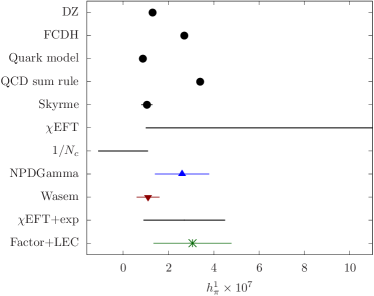
Figure 1: Collection of estimates of the nucleon-pion coupling $h^{1}_{\pi}$; extension of Fig. 4 in  [2] and Table I in  [1]. The labels match to references: DZ [4], FCDH [5], Quark model [10], QCD sum rule [11], Skyrme [9], $1/N_{c}$  [12], $\chi$EFT  [13], $\chi$EFT + exp [16], NPDGamma [2], LQCD [15], Factor+LEC [17]. The estimate for $\chi$EFT 2015 extends beyond the shown $h^{1}_{\pi}$ axis range $1.1\,(1.0)\cdot 10^{-6}$.

The above results are summarized in Fig. 1. We find this situation of scattered results highlights the need for systematic study and improved ab-initio theoretical determinations.

The aforementioned first ab-initio lattice QCD determination and the non-perturbative estimate of the nucleon matrix elements with the parity-violating (PV) effective Lagrangian has been presented in Ref. [15]. In this work the actual transition matrix elements $N\pi\overset{\mathcal{L}_{\mathrm{PV}}}{\longrightarrow}N$ for a transition of a nucleon-pion state to a nucleon state mediated by the $\Delta I=1$, parity-violating Lagrangian was considered. Though this calculation is pioneering, it is also exploratory in many regards as also discussed in detail in Refs. [18, 1]. Challenges are the rigorous treatment of the pion-nucleon state in finite volume and energy non-conservation between initial and finial state on the lattice, which were circumvented in Ref. [15]. Apart from this the calculation considered also only a certain quark flow diagram topology, arguing that the neglected diagrams are expected to have a contribution only within the statistical accuracy. Moreover, renormalization of the 4-quark operators was not included. Still, the obtained value on a coarse lattice with a heavier-than-physical pion $m_{\pi}\approx 390\,\mathrm{MeV}$ is consistent with the recent NPDGgamma experimental analysis.

An alternative theoretical ansatz has been put forward anew in Refs. [19, 1], by proposing a joint effort of chiral effective field theory ($\chi$EFT) and lattice QCD. Based on the PCAC relation the transition via the parity-violating interaction Lagrangian with a soft pion in the initial or final state is equivalent to a transition via a parity-conserving Lagrangian without a soft pion. Details on the relevant PCAC relation

$$\lim\limits_{p_{\pi}\to 0}\,\langle n\,\pi^{+}\,|\,\mathcal{L}^{w}_{\mathrm{PV}}(0)\,|\,p\rangle \approx-\frac{\sqrt{2}\,i}{F_{\pi}}\,\langle p\,|\,\mathcal{L}^{w}_{\mathrm{PC}}\,|p\rangle$$ (2)

are provided in Refs. [19, 1]. The PCAC relation Eq. (2) is, however, exact only in the limit of exact chiral symmetry. At non-zero pion mass it receives higher order corrections in $\chi$EFT. But these corrections can be argued to be numerically small [1], at the level of $\mathcal{O}\left({1\%}\right)$ at the physical pion mass, and can in principle also be calculated by studying the pion mass dependence with lattice QCD, based on known low-energy constants from meson and heavy-baryon chiral perturbation theory [19].

This alternative theoretical ansatz leads to a major simplification in the lattice computation: one now considers a transition amplitude between single nucleon states $N\overset{\mathcal{L}_{\mathrm{PC}}}{\longrightarrow}N$ with a parity-conserving (PC) Lagrangian, which from a numerical point of view is more straightforward to handle in a lattice calculation. In particular, the complication arising from the pion-nucleon state is absent since the matrix element is computed for single nucleon initial and final states.

In this work we investigate the computational concepts proposed in Ref. [1] in practice and propose a concrete numerical implementation to evaluate the nucleon 3-point functions with the 4-quark operator insertions of $\mathcal{L}_{\mathrm{PC}}$. Of course the ensuing Wick contractions still comprise fermion loop diagrams, which were neglected in the first work [18]. We will argue that these diagrams and the renormalization procedure are intricately linked: in the lattice calculation these particular fermion loop diagrams generate power-divergent mixing with lower-dimensional operators, and we add an initial discussion about such power divergent terms and our future strategy for renormalizing the 4-quark operators.

Preliminary results of this work have been reported in [20, 21].

II Operators and coupling

The matching between the parity-violating interaction in the electro-weak sector of the SM and the effective nucleon and pion degrees of freedom at energy scale $\Lambda_{\mathrm{QCD}}\sim m_{\mathrm{proton}}$ has been worked out in Ref. [22]. Here, we largely follow the notation of the recent Ref. [1]. The $\Delta I=1$, parity-conserving Lagrangian is given by

$$\mathcal{L}^{w}_{\mathrm{PC}} =-\frac{G_{F}}{\sqrt{2}}\,\frac{\sin^{2}\left(\theta_{w}\right)}{3}\,\sum\limits_{i}\,\left(C^{(1)}_{i}\,\theta^{(\ell)\prime}_{i}+S^{(1)}_{i}\,\theta^{(s)\prime}_{i}\right)\,,$$ (3)

$C^{(1)}$ and $S^{(1)}$ denote the Wilson coefficients obtained in 1-loop perturbation theory [22, 23].
The parity-even 4-quark operators $\theta^{(\ell)\prime}$ with only light quarks $\ell$ contributing and $\theta^{(s)\prime}$ with light and strange $s$ quarks contributing read

$$\theta^{(\ell)\prime}_{1} =\bar{q}_{a}\,\gamma_{\mu}\,\mathbb{1}\,q_{a}\,\bar{q}_{b}\,\gamma^{\mu}\,\tau^{3}\,q_{b}\,,$$

$$\theta^{(\ell)\prime}_{2} =\bar{q}_{a}\,\gamma_{\mu}\,\mathbb{1}\,q_{b}\,\bar{q}_{b}\,\gamma^{\mu}\,\tau^{3}\,q_{a}\,,$$

$$\theta^{(\ell)\prime}_{3} =\bar{q}_{a}\,\gamma_{\mu}\,\gamma_{5}\,\mathbb{1}\,q_{a}\,\bar{q}_{b}\,\gamma^{\mu}\gamma_{5}\,\tau^{3}\,q_{b}\,,$$

$$\theta^{(s)\prime}_{1} =\bar{s}_{a}\,\gamma_{\mu}\,s_{a}\,\bar{q}_{b}\,\gamma^{\mu}\,\tau^{3}\,q_{b}\,,$$

$$\theta^{(s)\prime}_{2} =\bar{s}_{a}\,\gamma_{\mu}\,s_{b}\,\bar{q}_{b}\,\gamma^{\mu}\,\tau^{3}\,q_{a}\,,$$

$$\theta^{(s)\prime}_{3} =\bar{s}_{a}\,\gamma_{\mu}\,\gamma_{5}\,s_{a}\,\bar{q}_{b}\,\gamma^{\mu}\gamma_{5}\,\tau^{3}\,q_{b}\,,$$

$$\theta^{(s)\prime}_{4} =\bar{s}_{a}\,\gamma_{\mu}\,\gamma_{5}\,s_{b}\,\bar{q}_{b}\,\gamma^{\mu}\gamma_{5}\,\tau^{3}\,q_{a}\,.$$ (4)

In the operator list Eq. (4) $q=(u,d)^{T}$ is the up and down quark doublet and $\tau^{3}$ is the third Pauli matrix, which gives the iso-vector combination $\bar{u}u-\bar{d}d$. As a perturbative addition to pure QCD, the interaction Lagrangian Eq. (3) induces a proton-neutron mass splitting $(\delta m_{N})_{4q}$ due to the 4-quark operators,

$$\left(\delta m_{N}\right)_{4q} =\frac{1}{m_{N}}\,\langle p\,|\,\mathcal{L}^{w}_{\mathrm{PC}}(0)\,|\,p\rangle=-\frac{1}{m_{N}}\,\langle n\,|\,\mathcal{L}^{w}_{\mathrm{PC}}(0)\,|\,n\rangle\,,$$ (5)

and with the PCAC relation the leading contribution to the coupling comes from the mass splitting

$$h^{1}_{\pi}\approx-\frac{1}{F_{\pi}}\,\frac{(\delta m_{N})_{4q}}{\sqrt{2}}\,,$$ (6)

where $F_{\pi}$ denotes the pion decay constant in the chiral limit.

In the following this work is mainly concerned with the lattice QCD estimate of the operator matrix elements $\langle N\,|\,\theta^{(f)}_{i}(0)\,|\,N\rangle$ for $f=\ell,\,s$ and $N$ the proton and neutron.

III 4-quark operator matrix elements from the lattice

To determine the nucleon matrix elements of the 4-quark operators in Eq. (4) we follow the Feynman-Hellmann-Theorem technique advocated for in Ref. [24]. The relevant correlation functions result from inserting the individual operators $\theta^{(f)\prime}_{i}(x)$ into the proton or neutron 2-point function, summed over all lattice sites $x$.

The nucleons are interpolated by the usual zero-momentum, positive parity proton and neutron 3-quark operators

$$N^{+}_{\alpha}(t) =P^{(+)}_{\alpha\alpha^{\prime}}\,\sum\limits_{\vec{y}}\,\epsilon_{abc}\,u_{a}(t,\vec{y})^{T}\,C\gamma_{5}\,d_{b}(t,\vec{y})\,\,u_{\alpha^{\prime}c}(t,\vec{y})$$

$$N^{0}_{\alpha}(t) =P^{(+)}_{\alpha\alpha^{\prime}}\,\sum\limits_{\vec{y}}\,\epsilon_{abc}\,d_{a}(t,\vec{y})^{T}\,C\gamma_{5}\,u_{b}(t,\vec{y})\,\,d_{\alpha^{\prime}c}(t,\vec{y})$$ (7)

with (positive) parity projector $P^{(+)}=\frac{1}{2}\,\left(\mathbb{1}+\gamma_{0}\right)$ and $C$ the charge conjugation matrix.

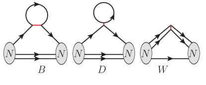
Figure 2: Quark flow diagrams from inserting 4-quark operators into the nucleon 2-point function. The red bar denotes the single-point vertex.

From these we construct the 2- and 3-point functions

$$C_{2pt}(t) =\mathrm{Tr}\left[\langle N(t+t_{i})\,\,\bar{N}(t_{i})\rangle\right]\,,$$ (8)

$$C_{3pt}(t) =\sum\limits_{x}\,\,\mathrm{Tr}\left[\langle N(t+t_{i})\,\,\theta^{(f)\prime}_{i}(x)\,\,\bar{N}(t_{i})\rangle\right]\,.$$ (9)

The different types of Wick contractions following from Eq. (9) are depicted in Fig. 2 in diagrammatic form. We distinguish three types of diagrams: those containing quark loops, denoted $B$ and $D$, and without a quark loop, denoted $W$. Note that the latter type is the only one included in the calculation of Ref. [18]. For the quark loop diagrams, we further make a technical distinction between type $D$, where the fermion loop is individually spin-color traced and type $B$, where it is not.

Quark-disconnected diagrams are neglected, since by virtue of the $\tau^{3}$ flavor structure of the operators in Eq. (4) such diagrams cancel in SU$(2)$ flavor symmetric QCD, which we work in.

We connect the 2- and 3-point functions in Eqs. (8), (9) to the nucleon matrix element by spectral decomposition and the Wigner-Eckart-Theorem

$$C_{2pt}(t) =\sum\limits_{\sigma}\,\mathrm{e}^{-m_{N}t}\frac{\mathrm{Tr}\left[\langle 0\,|\,N(0)\,|\,n,\sigma\rangle\,\langle n,\sigma\,|\,\bar{N}(0)\,|\,0\rangle\right]}{2m_{N}}$$

$$\qquad+\dots$$ (10)

$$C_{3pt}(t) =(t/a+1)\,\frac{\langle n\,|\,\,\theta^{(f)\prime}_{i}\,\,|\,n\rangle}{2m_{N}}\,\mathrm{e}^{-m_{N}t}$$ (11)

$$\times\sum\limits_{\sigma}\,\frac{\mathrm{Tr}\left[\langle 0\,|\,N(0)\,|\,n,\sigma\rangle\,\langle n,\sigma\,|\,\bar{N}(0)\,|\,0\rangle\right]}{2m_{N}}+\dots\,.$$

Here $|0\rangle$ denotes the QCD vacuum state , $|n,\sigma\rangle$ the nucleon ground state with zero 3-momentum and spin-1/2 component $\sigma$. In Eq. (11) we use the spin-independent matrix element

$$\langle n,\,\sigma\,|\,\,\theta^{(f)\prime}_{i}(0)\,\,|\,n,\,\sigma^{\prime}\rangle =\delta_{\sigma\,\sigma^{\prime}}\,\langle n\,|\,\,\theta^{(f)\prime}_{i}(0)\,\,|\,n\rangle\,,$$ (12)

for the Lorentz-scalar operator $\theta^{(f)\prime}_{i}$.

With ellipsis we denote excited state contributions as well as contributions from different time-orderings, which are at most of order $\mathcal{O}\left({t^{0}}\right)$. A detailed account of the application of the Feynman-Hellmann-Theorem (FHT) to the calculation of nucleon matrix elements can be found in Ref. [24].

According to FHT, in the vacuum $|\lambda\rangle$ including the perturbation $\lambda\,\mathcal{L}^{w}_{\mathrm{PC}}$ in the action we can determine the effective mass of the nucleon state for sufficiently large $t$ by

$$m_{\mathrm{eff}}^{(\lambda)}(t\,|\,\tau) =\frac{1}{\tau}\,\mathrm{arccosh}\left(\frac{C_{2pt}^{(\lambda)}(t+\tau)+C_{2pt}^{(\lambda)}(t-\tau)}{2\,C_{2pt}^{(\lambda)}(t)}\right)$$

$$=m_{\mathrm{eff}}(t\,|\,\tau)+\frac{\lambda}{2}\,(\delta m_{N})_{4q}+\mathcal{O}\left({\lambda^{2}}\right)\,,$$ (13)

up to excited state contamination, and $m_{\mathrm{eff}}$ as well as the matrix element for $(\delta m_{N})_{4q}$ are taken in pure QCD.

Taking the derivative with respect to $\lambda$ we then obtain the desired matrix element by studying the dependence on source-sink separation $t$ as well as offset $\tau$ of the ratio

$$R(t,\tau) =\frac{\xi}{\sqrt{\xi^{2}-1}}\times$$ (14)

$$\quad\times\frac{1}{\tau}\,\left(\frac{C_{3pt}(t+\tau)+C_{3pt}(t-\tau)}{C_{2pt}(t+\tau)+C_{2pt}(t-\tau)}-\frac{C_{3pt}(t)}{C_{2pt}(t)}\right)\,,$$

$$\overset{t\mathrm{~{}large}}{\longrightarrow}\frac{\langle n\,|\,\theta^{(f)\prime}_{i}\,|\,n\rangle}{2m_{N}}$$

$$\xi =\frac{C_{2pt}(t+\tau)+C_{2pt}(t-\tau)}{2C_{2pt}(t)}\,,$$

again up to excited state contamination. We determine $R$ per individual operator $\theta^{(f)\prime}_{i}$ by fitting the ratio to a constant for various ranges in $t$ and $\tau$.

Evaluation of diagrams

We evaluate the Wick contractions by a combination of point-to-all, stochastic and sequential quark propagators. The point-to-all propagators $\psi^{(x_{i},\alpha,a)}$ result from solving the lattice Dirac equation for a spin-color diluted source with support at a single lattice site

$$S^{\beta\alpha}_{ba}(x;x_{i}) ={D^{-1}}_{\beta,\beta^{\prime}}^{b,b^{\prime}}(x,y)\,\left[\delta_{x_{i},y}\,\delta_{\alpha,\beta^{\prime}}\,\delta_{a,b^{\prime}}\right]\,.$$ (15)

From the point-to-all propagators the nucleon 2-point functions are evaluated in the usual way.

The quark loop in diagrams $B$ and $D$ in Fig. 2 is constructed by a fully time, spin and color diluted stochastic timeslice propagator,

$$L(x)^{ab}_{\alpha\beta} =\sum\limits_{t,\gamma,c}\,{D_{u}^{-1}}_{\alpha\kappa}^{ad}(x;y)\,\,\left(\eta(t,\vec{y})\,\delta_{t_{y},t}\,\delta_{\gamma,\kappa}\,\delta_{d,c}\right)\times$$

$$\qquad\times\left(\eta(t,\vec{x})\,\delta_{t_{x},t}\,\delta_{\gamma,\beta}\,\delta_{b,c}\right)\,,$$ (16)

where $\eta(t,\vec{x})\,\in\,\left\{\pm 1\right\}$ are independent and identically with zero mean and unit variance

$$\mathrm{E}\left[\eta(t,\vec{x})\right] =0\,,\quad\mathrm{E}\left[\eta(t,\vec{x})\,\eta(t,\vec{y})\right]=\delta^{(3)}_{\vec{x},\vec{y}}\,.$$ (17)

To apply the FHT method we must sum the 3-point function with insertion of the 4-quark operator at each lattice site. We realize this summed simultaneous insertion by using the sequential inversion method: to that end we construct the two sequential sources for $B$- and $D$-type

$$S^{(B)}(x;x_{i}) =\Gamma\,L(x)\,\Gamma\,S(x;x_{i})\,,$$ (18)

$$S^{(D)}(x;x_{i}) =\mathrm{Tr}\left[\Gamma\,L(x)\right]\,\Gamma\,S(x;x_{i})\,.$$ (19)

Here $\Gamma$ is one of the relevant Dirac matrices $\Gamma=\gamma_{\mu}$ or $\Gamma=\gamma_{\mu}\gamma_{5}$. The Lorentz index $\mu$ is actually summed over at this stage.

By repeated inversion of the Dirac operators on these sources we obtain the sequential propagators $T^{(B)}$ and $T^{(D)}$ for $B$ and $D$ diagram, respectively, given by

$$T^{(K)}(y;x_{i}) =\sum\limits_{x}\,{D^{-1}}(y;x)\,S^{(K)}(x;x_{i})\,,\quad K=B,\,D\,.$$ (20)

The ensuing contractions for $C_{3pt}$ are analogous to those for $C_{2pt}$, using $T^{(B)}$ and $T^{(D)}$.

For the $W$ diagram in Fig. 2 we again use the stochastic sequential propagator technique to split the four quark lines connecting at the insertion point into two pairs. The relevant term of propagators through the insertion point then reads

$$\sum\limits_{x}\,S_{1}(y;x)\,\Gamma\,S_{1}(x;x_{i})\times S_{2}(y;x)\,\Gamma\,S_{2}(x;x_{i})$$ (21)

$$=\sum\limits_{x,z}\,S_{1}(y;x)\,\Gamma\,S_{1}(x;x_{i})\times S_{2}(y;z)\,\Gamma\,S_{2}(z;x_{i})\times\delta^{(4)}_{x,z}$$

$$=\sum\limits_{x,z}\,S_{1}(y;x)\,\Gamma\,S_{1}(x;x_{i})\times S_{2}(y;z)\,\Gamma\,S_{2}(z;x_{i})\times$$

$$\qquad\times\mathrm{E}\left[\eta(x)\,\eta(z)\right]\,,$$

with binary noise vector $\eta(x)$ as in Eq. (17), and subscript $1,2$ denoting the quark propagator flavor.

We thus generate a set of independent binary noise sources $\eta^{r},\,r=1,\dots,N_{r}$ as in Eq. (17), and the corresponding sequential sources and propagators

$$S^{(W),r}(x;x_{i}) =\Gamma\,\eta^{r}(x)\,S(x;x_{i})\,,$$

$$T^{(W),r}(y;x_{i}) =\sum\limits_{x}\,{D^{-1}}(y;x)\,S^{(W),r}(x;x_{i})\,,$$ (22)

and by Eq. (21) the product of two such sequential propagators from independent noise sources produces in the expectation value the four quark lines connected at a single site, which is summed over the lattice.

Fierz rearrangement

The operators in Eq. (4) fall into two classes with respect to their spin-color structure: $\theta^{(f)\prime}_{1}$ , $\theta^{(f)\prime}_{3}$ for $f=\ell,\,s$ consist of products of quark bilinear terms, i.e. $\bar{q}_{1}\,\Gamma\,q_{1}\times\bar{q}_{2}\,\Gamma\,q_{2}$. The remaining operators $\theta^{(\ell)\prime}_{2}$ and $\theta^{(s)\prime}_{2},\,\theta^{(s)\prime}_{4}$ have cross-linked color and spinor indices. We refer to those as “color-crossed” operators for short.

These matrix elements of the color-crossed operators can be computed in two different ways. The first one is to compute the contractions corresponding to the color-crossed operators. This is achieved by using color dilution of the sequential sources $S^{(W),r}$ in Eq. (22): adding color indices $a,b,c$ we thus have

$$S^{(W),r,a}_{bc}(x;x_{i}) =\Gamma\,\eta^{r}(x)\,S_{ac}(x;x_{i})\,\delta_{a,b}\,.$$ (23)

The second way is to apply a Fierz rearrangement in order to transform the color-crossed operators into products of standard quark bilinear factors, thereby avoiding the need for color dilution. Then, the analogous methods discussed above for the non color-crossed operators are applied. For instance $\theta^{(\ell)\prime}_{2}$ is equivalently represented as

$$\theta^{(\ell)\prime}_{2} =u_{\alpha,a}^{*}\,\left(\gamma_{\mu}\right)_{\alpha\beta}\,u_{\beta,b}\,u_{\gamma,b}^{*}\,\left(\gamma_{\mu}\right)_{\gamma\delta}\,u_{\delta,a}-\left[u\leftrightarrow d\right]$$

$$=\frac{1}{2}\,\bar{u}\,\gamma_{\mu}\,u\,\,\bar{u}\,\gamma_{\mu}\,u+\frac{1}{2}\,\bar{u}\,\gamma_{\mu}\gamma_{5}\,u\,\,\bar{u}\,\gamma_{\mu}\gamma_{5}\,u$$

$$\quad-\bar{u}\,\mathbb{1}\,u\,\,\bar{u}\,\mathbb{1}\,u+\bar{u}\,\gamma_{5}\,u\,\,\bar{u}\,\gamma_{5}\,u-\left[u\leftrightarrow d\right]\,,$$ (24)

where by $\left[u\leftrightarrow d\right]$ we denote the same term as written explicitly, but up replaced by down quark flavor. The strange operators are treated accordingly.

Thus, instead of the list of operators in Eq. (4), we consider only the quark bilinear forms

$$\bar{q}\,\Gamma\,q\,\,\bar{q}\,\Gamma\,q\,,\quad\bar{s}\,\Gamma\,q\,\,\bar{q}\,\Gamma\,s\,,\quad\bar{q}\,\Gamma\,q\,\,\bar{s}\,\Gamma\,s\,,\quad q=u,\,d$$ (25)

with as before $\Gamma=\left\{\gamma_{\mu}\right\},\,\left\{\gamma_{\mu}\gamma_{5}\right\}$, but also in addition $\Gamma=\mathbb{1},\,\gamma_{5}$.

IV Lattice computation

For our numerical study we use a gauge field ensemble from the Extended Twisted Mass Collaboration [25] with dynamical up, down, charm and strange quark. The ensemble has a lattice volume of $32^{3}\times 64$, a lattice spacing of $a\approx 0.091\ \mathrm{fm}$ and, thus, a spatial lattice extend of $L=3.1\ \mathrm{fm}$. The pion mass value is $m_{\pi}=261(1)\ \mathrm{MeV}$, $m_{\pi}\cdot L=4$ and the nucleon mass value is $m_{N}=1028(4)\ \mathrm{MeV}$. The strange quark mass is tuned to its physical value.

The simulated action features a light mass degenerate quark doublet of twisted mass fermions at maximal twist guaranteeing $O(a)$ improvement [26], amended by a Sheikholeslami-Wohlert “clover” term included to reduce residual $a^{2}$ lattice artifacts. The charm-strange doublet is again of twisted mass type, including a quark mass splitting term [27]. The heavy doublet action is not flavor diagonal, which needlessly complicates the calculation of correlation functions involving strange quarks. For the present study we thus use a mixed-action approach, by the addition of a doublet of Osterwalder-Seiler (OS) strange quarks [28], analogous to the light quark doublet.

The bare OS strange quark mass value, which is not critically important yet for this exploratory investigation, has been tuned such that the $\Omega$ baryon mass assumes its physical value.

The lattice action determines symmetry properties in our computation and these are relevant for the discussion of renormalization and mixing. We thus reprint the detailed formulas for sea and valence quark action in the App. A.

We summarize the statistics produced with the twisted mass gauge field ensemble for the evaluation of the individual diagrams from the 4-quark operator insertion in Tab. 1.

Diagram type	$N_{\mathrm{conf}}$	$N_{\mathrm{sample}}$	$N_{\mathrm{source}}$
$BD$	1262	768	2
$W$ Fierz-Id	1262	8	2
$W$ color-crossed	604	8	1

Table 1: Summary of statistics produced for the evaluation of the individual diagram types from the 4-quark operators inserted into the nucleon 2-point function. $N_{\mathrm{conf}}$ gives the number of independent gauge configurations, $N_{\mathrm{sample}}$ the number of stochastic samples and $N_{\mathrm{source}}$ the number of point sources employed in the estimates.

Contributions from $B$ and $D$ diagram type

For later discussion it will be valuable to consider the contribution to the nucleon 3-point functions for the individual operators from the combined $B$ and $D$ diagram type and the $W$-type separately, motivated by the fermion loop present in $B$ and $D$-type diagrams, but not in $W$-type diagrams.

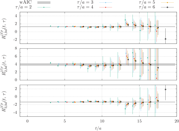
Figure 3: Estimates of $B$ and $D$ diagram contribution to the matrix element from the ratios Eq. (14), for various pairs $(t,\,\tau)$ with the weighted fit as gray band.

To determine the estimate for the matrix element we fit the ratios $R(t,\tau)$ to a constant in various ranges $t_{\mathrm{min}}\leq t\leq t_{\mathrm{max}}$ together with various sets $\left\{\tau_{1},\dots,\tau_{n}\right\}$ of joint data sets.

The fits are correlated with a block-diagonal covariance matrix, where we neglect the correlation between different $\tau$-values, i.e. we set $\mathrm{cov}\left(R(t,\tau)\,,\,R(t^{\prime},\tau^{\prime})\right)=0$ for all pairs $\tau\neq\tau^{\prime}$. Including cross-$\tau$ elements renders the covariance matrix near-singular and distorts the fit with bad estimates of said elements.

To each fit we assign an Akaike Information Criterion (AIC) weight following the procedure in Ref. [29], which is given by

$$w_{\mathrm{fit}} =\exp\left(-\frac{1}{2}\,(\chi^{2}+2\,N_{\mathrm{param}}-N_{\mathrm{data}})\right)$$ (26)

with $\chi^{2}$ based on the block-diagonal covariance matrix, $N_{\mathrm{param}}$ the number of fit parameters (one for our fit to constant), and $N_{\mathrm{data}}$ the number of data points ( $R(t,\tau)$ values ) entering the fit.

Moreover, the fits are bootstrapped and we obtain the fit parameter uncertainty from the variance over bootstrap samples. The ranges for $t$ and $\tau$ applied in the fits are given by

$$1\leq t_{\mathrm{min}}/a\leq 10\,,\quad 10\leq t_{\mathrm{max}}/a\leq 17\,,\quad 2\leq\tau/a\leq 6\,.$$ (27)

The boundaries are based on observation, where a meaningful fit is accessible, and given our current accuracy the above choice covers all such ranges. Note in addition, with the symmetric ratio in Eq. (14), the maximal addressed ratio value involves data at $t_{\mathrm{max}}+\tau$.

Finally, we restrict the set of parameters in our fits to a single constant (for the matrix element). At present level of statistical uncertainty per $R(t,\tau)$ data point, in most $t/\tau$ ranges we cannot model excited state contamination in our data with any statistical significance.

From all available fits with best fit parameter $\mu_{i}$ and error $\sigma_{i}$ and AIC weight $w_{i}$ we build the combined distribution function [29]

$$\mathrm{CDF}(x) =\sum\limits_{i}\,w_{i}\,\mathcal{N}_{\mu_{i},\sigma_{i}}(x)/\sum\limits_{j}\,w_{j}\,.$$ (28)

$\mathcal{N}_{\mu,\sigma}$ is the normal distribution with mean $\mu$ and variance $\sigma^{2}$. Based on $\mathrm{CDF}(x)$ we quote the median of the distribution function as the central value and the $16\%$ and $84\%$ quantiles as the uncertainty interval.

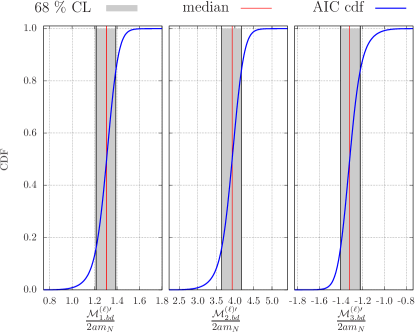
Figure 7: Cumulative distribution function built from AIC weights, for $\theta^{(\ell)\prime}_{k}$ matrix element $\mathcal{M}^{(\ell)\prime}_{k}$; the AIC-based cumulative distribution function is shown as the blue line, the ensuing median in red; the gray shaded band is bounded by the $16\%$ and $84\%$ quantiles.

In Fig. 3 we present the ratio $R^{(\ell)^{\prime}}(t,\tau)$ as a function of $t$ for different values of $\tau$ for the $B$ and $D$-type operators. In addition we include the result of the AIC weighting procedure as gray bands. The distribution functions and quantiles corresponding to the AIC procedure are shown in Fig. 7 in App. B.

Contributions from $W$ diagram type

The analysis of the $W$ diagram contribution proceeds analogously to the $B+D$ case.

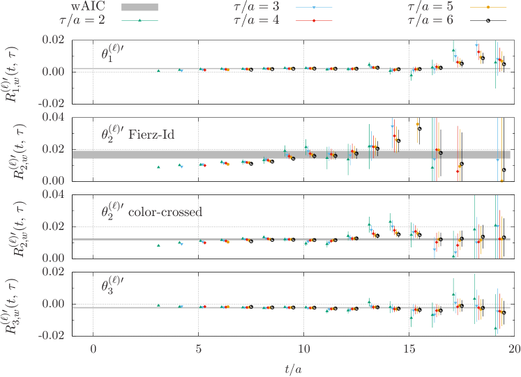
Figure 4: Estimates of $W$ diagram contribution to the matrix element from the ratios Eq. (14); the meaning of symbols as Fig. 3.

We show the ratio data $R(t,\tau)$ per operator in Fig. 4 with our estimate for the matrix element as the gray band. Fig. 4 (App. B) correspondingly justifies this estimate at the level of the cumulative distribution function.

Diagrams with strange quarks

For the strange operators $\theta^{(s)\prime}$ in Eq. (4), only one diagram type contributes per operator. These are $D$-type contributions for $\theta^{(s)\prime}_{1,\,3}$ and $B$-type contributions for $\theta^{(s)\prime}_{2,\,4}$, the latter only when using Fierz rearrangement for these two operators. Still, whether $B$ or $D$, only strange quark loop diagrams occur in this case.

Here, we circumvent the technical complication of unitary strange and charm flavor mixing by the twisted mass heavy quark action Eq. (39) and employ the aforementioned mixed action approach with a strange quark doublet $(s_{+},\,s_{-})$, analogously to the light quark doublet.

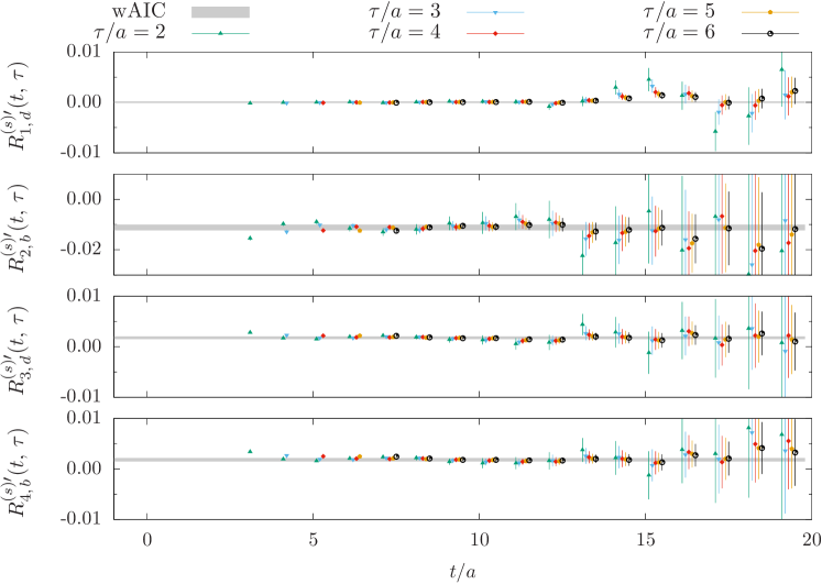
Figure 5: Strange operator ratios $R^{(s)\prime}$ and matrix element fits for operators $\theta^{(s)\prime}$.

This means the strange operators matrix elements are determined similarly to the one for $\theta^{(\ell)\prime}$, with the replacement of the light quark loop by the strange quark loop, $L_{u}(x)\to L_{s}(x)$. Since the two strange quark flavors in the doublet $(s_{+},\,s_{-})$ are identical in the continuum limit, we insert the strange quark loop averaged over both strange quark flavors. Using $\gamma_{5}$-hermiticity, in detail we then define

$$\bar{L}_{s}(x) =\frac{1}{2}\,\left(L_{s_{+}}+L_{s_{-}}\right)=\frac{1}{2}\,\left(L_{s_{+}}+\gamma_{5}\,L_{s_{+}}^{\dagger}\,\gamma_{5}\right)\,,$$ (29)

$$L_{s_{\pm}} =D_{s_{\pm}}^{-1}\,\eta\,\eta^{t}\,.$$

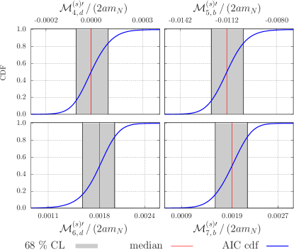
Figure 9: Strange operator AIC analysis by cumulative distribution function.

We show the lattice data and the matrix element fit result for the ratios $R^{(s)\prime}(t,\tau)$ in Fig. 5. The application of the AIC cumulative distribution functions defined in Eq. (28) is shown in Fig. 9 in App. B.

Discussion of matrix elements from BDW diagrams

All results for the matrix elements are compiled in Tabs. 2 for light quark operators and 3 for the strange quark operators. They are given per operator flavor $f=\ell,\,s$, operator number $k$ and as a third label we give the diagrams contributing.

$(f,\,k,\,X)$	$(\ell,\,1,\mathrm{bd})$	$(\ell,\,2,\mathrm{bd})$	$(\ell,\,3,\mathrm{bd})$	$(\ell,\,1,\mathrm{w})$	$(\ell,\,2,\mathrm{w})$	$(\ell,\,3,\mathrm{w})$
$\mathcal{M}^{(f)\prime}_{k,\,X}/(2am_{N})$	$1.307\,_{-0.094}^{+0.082}$	$3.93\,_{-0.28}^{+0.25}$	$-1.320\,_{-0.085}^{+0.097}$	$0.218\,_{-0.017}^{+0.019}\cdot 10^{-2}$	$1.66\,_{-0.21}^{+0.24}\cdot 10^{-2}$	$-0.218\,_{-0.025}^{+0.022}\cdot 10^{-2}$

Table 2: Summary of best estimates for dimensionless bare operator matrix elements per diagram type $B+D$ (“bd”) and $W$ (“w”), divided by $2m_{N}$, from our fits and AIC analysis.

$(f,\,k,\,X)$	$(s,\,1,\mathrm{d})$	$(s,\,2,\mathrm{b})$	$(s,\,3,\mathrm{d})$	$(s,\,4,\mathrm{b})$
$\mathcal{M}^{(f)\prime}_{k,\,X}/(2am_{N})$	$0.002\,_{-0.008}^{+0.010}\cdot 10^{-2}$	$-1.117\,_{-0.100}^{+0.107}\cdot 10^{-2}$	$0.182\,_{-0.024}^{+0.021}\cdot 10^{-2}$	$0.185\,_{-0.032}^{+0.029}\cdot 10^{-2}$

Table 3: Summary of best estimates for dimensionless bare strange operator matrix elements, divided by $2m_{N}$, from our fits and AIC analysis.

In Tab. 2 we observe a difference in magnitude between $B+D$ and $W$ diagram contributions for each individual operator by two orders of magnitude. Our explanation here mixing with operators of lower (and equal) mass-dimension, in the case of $B$ and $D$ diagrams. The latter two types contain a quark loop and we argue in Sec. VI below, that mixing of the 4-quark operator is permitted, starting with local quark-bilinear operators. By naive visual inspection, the structure of the $W$ diagram on the other hand, does not allow for such mixing and in Sec. V below we use solely its contribution to arrive at an estimate of $h^{1}_{\pi}$ in analogy to Ref. [18].

The strange quark operators $\theta^{(s)\prime}_{k}$ are entirely built from $B$- and $D$-type diagrams, albeit with the strange quark flavor running inside the fermion loop. These operators are therefore equally prone to mixing as the light quark operators.

This mixing of $\left\{\theta^{(\ell)\prime}_{k},\,\theta^{(s)\prime}_{k}\right\}$ in lattice QCD with lower dimensional operators does not come entirely unexpected, given the dimension 6 of the operators and the reduced symmetry of the lattice model. We add several comments on potential subtractions and renormalization in Sec. VI below.

A second feature is the antisymmetry of $\mathcal{M}^{(\ell)\prime}_{1}$ and $\mathcal{M}^{(\ell)\prime}_{3}$. The opposite-equal values can be shown for the bare matrix element at tree-level of perturbation theory. Beyond that, we are currently unaware of a symmetry argument, that would enforce this property at the non-perturbative level.

V Bare coupling from $W$-type diagram

We put our present study in perspective to the work of Ref. [15] by taking an analogous approach: we only include the contribution from the $W$-type diagram and ignore the multiplicative renormalization and the mixing to match the lattice result to the $\overline{MS}$ scheme, while still using the Wilson coefficients from renormalized perturbation theory.

Thus, we evaluate the combination of matrix elements $\mathcal{M}^{(\ell)\prime}_{i}=\langle N\,|\,\theta^{(\ell)\prime}_{i}\,|\,N\rangle/(2m_{N})$

$$\mathcal{M}_{C} =\sum\limits_{i=1}^{3}\,C^{(1)}_{i}\,\mathcal{M}^{(\ell)\prime}_{i}\,.$$ (30)

Based on the sets of bootstrapped fits with their associated AIC weights, we construct the cumulative distribution function for $\mathcal{M}_{C}$ by first building all combinations of fits for $\mathcal{M}^{(\ell)}_{i}$, $i=1,2,3$, then determining the mean and error from bootstrap mean and variance of the sample-wise built linear combination in Eq. (30), and finally assigning to each such combination of fits the AIC weight as the product of weights from the three individual matrix element fits.

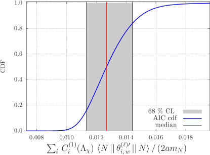
Figure 6: Cumulative distribution function for the combined estimate of $\mathcal{M}_{C}$ in Eq. (30).

The resulting cumulative distribution function is shown in Fig. 6, together with the median ($\alpha=0.5$ quantile) and the confidence band from the $\alpha=0.16,\,0.84$ quantiles.

From the matrix element estimate $\mathcal{M}_{C}$ we determine the bare coupling based on the $W$-type diagrams by multiplying the numerical factors from the effective Lagrangian.

$$h^{1}_{\pi}\left(W,\,\mathrm{bare}\right) =\frac{G_{F}\cdot(\hbar c/a)^{2}\,\sin^{2}(\theta_{W})}{3\,af_{\pi}}$$

$$\qquad\times\ \frac{a^{4}\,C^{(1)}_{i}\,\langle N\,|\,\theta^{(\ell)\prime}_{i}(0)\,|\,N\rangle}{2\,am_{N}}$$ (31)

In Eq. (31) we restored all explicit factors of the lattice spacing $a$ to have dimensionless quantities only.

The pion decay constant for the gauge field ensemble considered has been determined in Ref. [30] with value in lattice units $af_{\pi}=0.06674\,(15)$. The only explicit use of the lattice spacing is made to convert the Fermi constant $G_{F}$ as an external scale to lattice units. We use the value $a=0.09076\,(54)\,\mathrm{fm}$ from Ref. [31].

For the matrix elements combined with the Wilson coefficients in lattice units we find

$$\frac{a^{4}\,C^{(1)}_{i}\,\langle N\,|\,\theta^{(\ell)\prime}_{i}(0)\,|\,N\rangle}{2\,am_{N}} =1.27\,_{13}^{17}\cdot 10^{-2}\,,$$ (32)

and together with the conversion factor with Standard Model parameters from PDG [32] converted to lattice units

$$\frac{G_{F}\cdot(\hbar c/a)^{2}\,\sin^{2}(\theta_{W})}{3\,af_{\pi}} =6.367\,(77)\cdot 10^{-5}\,,$$ (33)

the result for the bare coupling is then

$$h^{1}_{\pi}\left(W,\,\mathrm{bare}\right) =8.08\,(98)\cdot 10^{-7}\,.$$ (34)

The result in Eq. (34) as representative of a lattice estimate of $h^{1}_{\pi}$ is by construction very preliminary. Conceptually, in its underlying restrictions it is similar to the first lattice determination in Ref. [18], which found

$$h^{1}_{\pi}\left(\mathrm{Wasem~{}2012}\right) =(1.099\pm 0.505)\,^{+0.058}_{-0.064}\cdot 10^{-7}\,,$$ (35)

at $m_{\pi}\approx 389\,\mathrm{MeV}$ pion mass and with a coarser lattice $a=0.123\,\mathrm{fm}$. We recall, that the computational ansatz of both lattice calculations differs fundamentally in using a parity-violating versus parity-conserving interaction Lagrangian.

Moreover, our preliminary result for $h^{1}_{\pi}(W,\,\mathrm{bare})$ is of compatible by order of magnitude with the recent experimental value

$$h^{1}_{\pi}(\mathrm{exp}) =2.6\,(1.2)_{\mathrm{stat}}\,(0.2)_{\mathrm{syst}}\cdot 10^{-7}\,.$$ (36)

VI Comments on mixing and outline of renormalization

The renormalization of the set of 4-quark operators in Eq. (4) in continuum QCD has been discussed in Refs. [22, 23], and finds its expression in the Wilson coefficients $\left\{C^{(1)}_{i},\,S^{(1)}_{i}\right\}$ which are calculated in renormalized QCD perturbation theory in the $\overline{\mathrm{MS}}$ scheme, together with their anomalous dimension matrix. In continuum QCD with the mass-independent $\overline{\mathrm{MS}}$ scheme and dimensional regularization, mixing with operators of lower dimension is excluded.

Here we comment on the situation in the practical lattice QCD calculation, with Wilson-type fermions and non-zero quark mass. The explicit breaking of proper Lorentz symmetry down to discrete 3-rotations and to non-equivalence of spatial and temporal direction (due to $T\neq L$) does not play a significant role for the 4-quark operators, which are invariant under a 3- and 4-dimensional rotation.

Of practical importance in this numerical calculation with Wilson-type fermions is the breaking of chiral symmetry, of up-down SU(2) flavor and parity symmetry. We focus in these introductory remarks on the light quark propagators $\theta^{(\ell)\prime}$.

Twisted Mass fermions

The symmetries of the twisted mass lattice action for the light quarks are listed in Eqs. (40), (41), (42), (43), (44) and (45) in the App. A.

Based on these lattice symmetries we identify the operators which are allowed to mix, i.e. which are not excluded by quantum numbers under those symmetry transformations. These quantum numbers are for the (light) 4-quark operators

Operator	$\mathcal{P}\mathcal{D}[-m_{f}]$	$\mathcal{T}\mathcal{D}[-m_{f}]$	$\mathcal{C}$	$\mathcal{D}\mathcal{R}_{5}$	$\mathcal{P}\mathcal{S}$
$\theta^{(\ell)\prime}$	$+1$	$+1$	$+1$	$+1$	$-1$

The mixing candidate operators of mass-dimension 3 to 5 are given by

dim
3	$\bar{q}\,\gamma_{5}\otimes\mathbb{1}\,q$
4	$m_{\ell}\,\bar{q}\,\mathbb{1}\otimes\tau^{3}\,q$,    $\bar{q}\,\not{D}\otimes\tau^{3}\,q$
5	$m_{\ell}^{2}\,\bar{q}\,\gamma_{5}\otimes\mathbb{1}\,q$ ,   $m_{\ell}\,\bar{q}\,\gamma_{5}\not{D}\otimes\mathbb{1}\,q$,
	$\bar{q}\,\gamma_{5}\,D^{2}\otimes\mathbb{1}\,q$,    $\bar{q}\,\sigma_{\mu\nu}\,\tilde{G}_{\mu\nu}\,q$,   $m_{\ell}\,G\tilde{G}$

Here, $\mathbb{1}$ denotes the unit matrix in spinor and flavor space, respectively, and $\tilde{G}_{\mu\nu}=\epsilon_{\mu\nu\alpha\beta}\,G_{\alpha\beta}$ the dual (lattice) gluon field strength tensor. The dimension-3 operator is allowed by breaking of parity $\mathcal{P}$ symmetry by the twisted mass fermion action. The dimension-4 operators are allowed by chiral symmetry breaking, which in addition to having opposite $\mathcal{R}_{5}$ parity to $\theta^{(\ell)\prime}$ is indicated by the explicit factor of the fermion mass $m_{\ell}$. Both operators are connected by the equation of motion for the quark field. Analogous statements hold for the dimension-5 operators.

Mixing with such operator matrix elements hampers the extraction of the renormalized 4-quark operator matrix elements in the continuum limit, due to power-divergent mixing coefficients $1/a^{3}$ and $1/a^{2}$ for dimension-3 and -4 operators, respectively. A suitable scheme to subtract such contributions appears to be the gradient flow together with the short flow time expansion [33]. The practical application to the twisted mass case is currently under investigation.

We mention two other setups, which are of interest in this study of the method using parity-even 4-quark operators.

Iso-symmetric Wilson fermions

Wilson fermions observing SU(2) isospin symmetry have individual parity $\mathcal{P}$ and exchange symmetry $\mathcal{S}$ (cf. Eqs. (40)-(45)). What remains is the explicit chiral symmetry breaking by the Wilson term. In this case the dimension-3 operator is ruled out by parity symmetry. However, the dimension-4 operator $m_{\ell}\,\bar{q}\,\mathbb{1}\otimes\tau^{3}\,q$ (and thus the related $\bar{q}\,\not{D}\otimes\tau^{3}\,q$) is still allowed to mix.

Parity-odd 4-quark operators

This case was investigated in Ref. [15], with iso-symmetric clover-improved Wilson fermions. In this case, using parity $\mathcal{P}$, charge conjugation $\mathcal{C}$ and exchange symmetry $\mathcal{S}$ is sufficient to show, that there is no operator of dimension 3, 4 or 5, that can mix on the lattice with the operators of $\mathcal{L}_{\mathrm{PV}}^{w}$.

The different mixing properties in the lattice QCD calculation with Wilson-type fermion regularization appear as a major drawback of using the PCAC relation and converting to the parity-conserving Lagrangian. However, in the parity-violating case the accurate representation of the nucleon-pion state with the Lüscher method and the ensuing signal-to-noise problem from the meson-baryon interpolator pose potentially even harder problems, especially towards physical pion mass and large lattice volume.

VII Conclusion

In this work we investigated the numerical implementation of a new method to calculate nucleon matrix elements of parity-even flavor-conserving 4-quark operators from lattice QCD, that pertain to the fully theoretical prediction of the long-range nucleon-pion coupling $h^{1}_{\pi}$. This constitutes the first step towards a full-fledged calculation of the coupling from a combination of chiral perturbation theory and non-perturbative lattice matrix elements. For one ensemble at pion mass $260\,\mathrm{MeV}$ and lattice spacing $a\approx 0.091\,\mathrm{fm}$ we demonstrated for the first time the calculation of all relevant (bare) matrix elements at the level of $10\%$ combined statistical and systematic uncertainty. The specific implementation shown here is readily and feasibly scalable towards physical pion mass, continuum and infinite volume.

We achieve this result due to the simplified representation of the coupling by application of the soft-pion-theorem and the implied sufficiency to calculate (single-hadron) nucleon matrix elements of parity-even operators. Of course, corrections to this leading order defining relation in $\chi$PT, though expected to be small, can in principle be computed and, therefore, the approximation is systematically improvable.

However, renormalization of lattice matrix elements poses a challenge due to mixing with lower-dimensional operators.

$W$ light	$B+D$ light	$B+D$ strange
$1.27\,_{13}^{17}\cdot 10^{-2}$	$4.12\,_{20}^{20}$	$3.10\,_{29}^{25}\cdot 10^{-2}$

Table 4: Summary of matrix elements per diagram type, weighted by the Wilson coefficients.

To appreciate the expected impact of this mixing we summarize our results for the bare matrix elements normalized by twice the nucleon mass in lattice units and weighted by the Wilson coefficients in Tab. 4. In the table we keep the three contributions

$$\sum\limits_{i=1}^{3}\,C^{(1)}_{i}\,\mathcal{M}^{(\ell)^{\prime}}_{i,w}/(2am_{N})\,,\,\,\,\,\sum\limits_{i=1}^{3}\,C^{(1)}_{i}\,\mathcal{M}^{(\ell)^{\prime}}_{i,bd}/(2am_{N})\,,$$

$$\qquad\sum\limits_{i=1}^{4}\,S^{(1)}_{i}\,\mathcal{M}^{(s)^{\prime}}_{i,bd}/(2am_{N})\,,$$ (37)

separate, which are light operators with $W$-type diagrams, light operators with $B+D$-type diagrams and the light-strange operators with $B+D$-type diagrams. From our numerical investigation we find that only $W$ light has the expected order of magnitude, while the light and strange $B+D$-type diagram contributions are much larger. The latter two types contain fermionic loop sub-diagrams, which we deem as the origin of the mixing.

This mixing comes about due to reduced symmetries at non-zero lattice spacing and explicit breaking of chiral symmetry due to finite quark mass values. The Gradient Flow method for subtracting power-divergent mixing and renormalization appears as a promising direction to study, due to the possibility to study mixing and matching to a continuum renormalization scheme only after extrapolating lattice data to the continuum, and thus with restored symmetries. The investigation of its practical implementation for the pertinent 4-quark operators is our on-going work.

Appendix A Lattice action and symmetries

Light quark lattice action

The lattice action of up and down quark for twisted mass fermions with a clover term is given by

$$\mathcal{S}^{(\ell)} =a^{4}\;\sum\limits_{f=u,d}\;\sum\limits_{x}\;\bar{\psi}_{f}(x)\;\left(\gamma_{\mu}\,\bar{\nabla}_{\mu}-i\gamma_{5}\,W_{\mathrm{cr}}+m_{f}+r_{f}\,\frac{ac_{\mathrm{SW}}}{4}\,\gamma_{5}\,\sigma\,G\right)\;\psi(x)\,,$$ (38)

with Wilson parameters $r_{u}=1=-r_{d}$.

In Eq. (38) we have covariant derivative

$$\bar{\nabla}_{\mu} =\frac{1}{2}\,\left(\nabla^{f}_{\mu}+\nabla^{b}_{\mu}\right)\,,$$

the subtracted Wilson term of dimension 5

$$W_{\mathrm{cr}} =-\frac{a\,r_{f}}{2}\,\nabla^{f}_{\mu}\,\nabla^{b}_{\mu}+M_{\mathrm{cr}}(r_{f})\,,$$

and the Sheikholeslami-Wohlert term again of dimension 5 and with the clover-plaquette-based lattice field strength tensor $G$ [43].

The form of the twisted mass lattice action (38) is valid in the physical basis of the quark fields, i.e. where the mass term is real and diagonal, at maximal twist  [44], such that automatic $\mathcal{O}\left({a}\right)$ improvement is realized for physical observables.

Discretization of the strange quark fermion action

For the strange quark we employ the mixed action technique, with different fermion discretization used for the sea quarks pertaining to gauge field sampling and to the valence quark, used for the actual calculations of correlation functions.

The sea quark action is given in Ref. [28] and to realize a mass splitting and automatic $\mathcal{O}\left({a}\right)$ improvement features mixing strange and charm sea quark flavor by lattice artifacts.

$$\mathcal{S}^{(s,c)}_{\mathrm{sea}} =a^{4}\;\sum\limits_{x}\;\bar{\psi}_{h}(x)\;\left(\gamma_{\mu}\,\bar{\nabla}_{\mu}-i\gamma_{5}\,\tau^{1}\,W_{\mathrm{cr}}+\mu_{\sigma}+\mu_{\delta}\,\tau^{3}+\frac{ac_{\mathrm{SW}}}{4}\,\tau^{1}\,\gamma_{5}\,\sigma\,G\right)\;\psi_{h}(x)\,,$$ (39)

where $\psi_{h}=(c,\,s)^{T}$ denotes the strange-charm doublet, $\mu_{\sigma}$ the average bare quark mass of the doublet and $\mu_{\delta}$ the mass splitting. The bare mass parameters $\mu_{\sigma},\,\mu_{\delta}$ are tuned by the two conditions of physical $D_{s}$ meson mass, as well as the renormalized quark mass ratio $\left.m_{s}/m_{c}\right|_{\overline{\mathrm{MS}},\mu=2\,\mathrm{GeV}}$.

To simplify the calculation of nucleon correlators with strange operator insertion we follow the mixed action approach in Ref. [28] and introduce another doublet of twisted mass valence strange quarks $(s_{+},s_{-})$. It is formally identical to the light quark doublet, except for the value of the bare twisted quark mass $m_{\ell}\to m_{s}$.

In particular it shares the critical hopping parameter (as tuned to maximal twist), and the Sheikholeslami-Wohlert parameter $c_{\mathrm{SW}}$ with the light quark sector. The bare quark mass $m_{s}$ at maximal twist is given by twisted quark mass parameter $m_{s}=\mu_{s}$ and the latter is tuned, such that the mass of the $\Omega$ baryon takes the physical value.

Symmetry transformations for light quarks

We list the complete set of discrete transformations, which pertain to our identification of operator mixing for the 4-quark operators. Apart from those listed here, there are the 3-rotations, and the residual (continuous) $\text{U}(1)_{3}$ flavor symmetry, under which the lattice action is invariant.

The discrete transformations of charge conjugation $C$, parity $P$ and time reversal $T$ are given by

$$\psi(t,\vec{x}) \stackrel{{\scriptstyle C}}{{\to}}C^{-1}\,\bar{\psi}(t,\vec{x})^{T}\,,\quad\bar{\psi}(t,\vec{x})\stackrel{{\scriptstyle C}}{{\to}}-\psi(t,\vec{x})^{T}\,C$$

$$U_{\mu}(t,\vec{x}) \stackrel{{\scriptstyle C}}{{\to}}U_{\mu}(t,\vec{x})^{*}$$ (40)

$$\psi(t,\vec{x}) \stackrel{{\scriptstyle P}}{{\to}}\gamma_{4}\,\psi(t,-\vec{x})\,,\quad\bar{\psi}(t,\vec{x})\stackrel{{\scriptstyle P}}{{\to}}\bar{\psi}(t,-\vec{x})\,\gamma_{4}$$

$$U_{4}(t,\vec{x}) \stackrel{{\scriptstyle P}}{{\to}}U_{4}(t,-\vec{x})\,,\quad U_{k}(t,\vec{x})\stackrel{{\scriptstyle P}}{{\to}}U_{k}(t,-\vec{x}-a\hat{k})^{\dagger}$$ (41)

$$\psi(t,\vec{x}) \stackrel{{\scriptstyle T}}{{\to}}i\gamma_{4}\,\gamma_{5}\,\psi(-t,\vec{x})\,,\quad\bar{\psi}(t,\vec{x})\stackrel{{\scriptstyle T}}{{\to}}-i\bar{\psi}(-t,\vec{x})\,\gamma_{5}\,\gamma_{4}$$

$$U_{4}(t,\vec{x}) \stackrel{{\scriptstyle T}}{{\to}}U_{4}(-t-a,\vec{x})^{\dagger}\,,\quad U_{k}(t,\vec{x})\stackrel{{\scriptstyle T}}{{\to}}U_{k}(-t,\vec{x})$$ (42)

In addition to the discrete Lorentz transformation there are several spurious transformations

$$\mathcal{R}_{5} :\left\{\begin{matrix}\psi\to\gamma_{5}\,\psi\,,\quad\bar{\psi}\to-\bar{\psi}\,\gamma_{5}\end{matrix}\right\}$$ (43)

$$\mathcal{D}_{d} :\left\{\begin{matrix}\psi\to\mathrm{e}^{\frac{3}{2}\pi\,i}\,\psi\,,\quad\bar{\psi}\to\mathrm{e}^{\frac{3}{2}\pi\,i}\,\bar{\psi}\\ U_{\mu}(x)\to U_{\mu}(-x-a\hat{\mu})^{\dagger}\\ \end{matrix}\right\}$$ (44)

$$\mathcal{S}_{u,d} :\left\{\begin{matrix}u/d\to d/u\,,\quad\bar{u}/\bar{d}\to\bar{d}/\bar{u}\end{matrix}\right\}$$ (45)

The transformations (40), (41), (42), (43), (44) and (45) form a complete set to define the light quark action and form operator multiplets eligible for mixing. The following transformations are symmetries

$$P\times\mathcal{D}_{d}\times(m_{f}\to-m_{f})\,,$$ (46)

$$T\times\mathcal{D}_{d}\times(m_{f}\to-m_{f})\,,$$ (47)

$$\mathcal{C}\,,$$ (48)

$$\mathcal{D}_{d}\times\mathcal{R}_{5}\,,$$ (49)

$$P\times\mathcal{S}_{u,d}\,,$$ (50)

where the spurious transformation $m_{f}\to-m_{f}$ denotes the change of sign of the bare mass parameters.

Appendix B AIC cumulative distribution functions

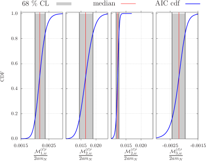
Figure 8: Cumulative distribution function built from AIC weights for $W$ diagram contribution.

References

- Guo and Seng [2019] F.-K. Guo and C.-Y. Seng, Effective Field Theory in The Study of Long Range Nuclear Parity Violation on Lattice, Eur. Phys. J. C 79, 22 (2019), arXiv:1809.00639 [nucl-th] .
- Blyth et al. [2018] D. Blyth et al. (NPDGamma), First Observation of -odd Asymmetry in Polarized Neutron Capture on Hydrogen, Phys. Rev. Lett. 121, 242002 (2018), arXiv:1807.10192 [nucl-ex] .
- Desplanques et al. [1980] B. Desplanques, J. F. Donoghue, and B. R. Holstein, Unified treatment of the parity violating nuclear force, Annals of Physics 124, 449 (1980).
- Dubovik and Zenkin [1986] V. M. Dubovik and S. V. Zenkin, Formation of Parity Nonconserving Nuclear Forces in the Standard Model SU(2)(l) X U(1) X SU(3)(c), Annals Phys. 172, 100 (1986).
- Feldman et al. [1991] G. B. Feldman, G. A. Crawford, J. Dubach, and B. R. Holstein, Delta contributions to the parity violating nuclear interaction, Phys. Rev. C 43, 863 (1991).
- Kaiser and Meißner [1988] N. Kaiser and U. G. Meißner, The Weak Pion - Nucleon Vertex Revisited, Nucl. Phys. A 489, 671 (1988).
- Kaiser and Meißner [1990] N. Kaiser and U. G. Meißner, Theoretical Aspects of Nuclear Parity Violation, Nucl. Phys. A 510, 759 (1990).
- Kaiser and Meißner [1989] N. Kaiser and U. G. Meißner, Novel Calculation of Weak Meson Nucleon Couplings, Nucl. Phys. A 499, 699 (1989).
- Meißner and Weigel [1999] U. G. Meißner and H. Weigel, The Parity violating pion nucleon coupling constant from a realistic three flavor Skyrme model, Phys. Lett. B 447, 1 (1999), arXiv:nucl-th/9807038 .
- Hyun et al. [2017] C. H. Hyun, H.-C. Kim, and H.-J. Lee, Parity-violating coupling constant from the flavor-conserving effective weak chiral Lagrangian, Phys. Lett. B 768, 130 (2017), arXiv:1607.06572 [hep-ph] .
- Lobov [2002] G. A. Lobov, Electroweak pion nucleon constant, Phys. Atom. Nucl. 65, 534 (2002).
- Phillips et al. [2015] D. R. Phillips, D. Samart, and C. Schat, Parity-Violating Nucleon-Nucleon Force in the 1/ Expansion, Phys. Rev. Lett. 114, 062301 (2015), arXiv:1410.1157 [nucl-th] .
- de Vries et al. [2015] J. de Vries, N. Li, U.-G. Meißner, A. Nogga, E. Epelbaum, and N. Kaiser, Parity violation in neutron capture on the proton: Determining the weak pion–nucleon coupling, Phys. Lett. B 747, 299 (2015), arXiv:1501.01832 [nucl-th] .
- de Vries and Meißner [2016] J. de Vries and U.-G. Meißner, Violations of discrete space–time symmetries in chiral effective field theory, Int. J. Mod. Phys. E 25, 1641008 (2016), arXiv:1509.07331 [hep-ph] .
- Wasem [2012a] J. Wasem, Lattice QCD Calculation of Nuclear Parity Violation, Phys. Rev. C 85, 022501 (2012a), arXiv:1108.1151 [hep-lat] .
- de Vries et al. [2020] J. de Vries, E. Epelbaum, L. Girlanda, A. Gnech, E. Mereghetti, and M. Viviani, Parity- and Time-Reversal-Violating Nuclear Forces, Front. in Phys. 8, 218 (2020), arXiv:2001.09050 [nucl-th] .
- Gardner and Muralidhara [2022] S. Gardner and G. Muralidhara, QCD analysis of hadronic parity violation, Phys. Lett. B 833, 137372 (2022), arXiv:2203.00033 [hep-ph] .
- Wasem [2012b] J. Wasem, Lattice QCD Calculation of Nuclear Parity Violation, Phys. Rev. C85, 022501 (2012b), arXiv:1108.1151 [hep-lat] .
- Feng et al. [2018] X. Feng, F.-K. Guo, and C.-Y. Seng, Novel Soft-Pion Theorem for Long-Range Nuclear Parity Violation, Phys. Rev. Lett. 120, 181801 (2018), arXiv:1711.09342 [nucl-th] .
- Sen et al. [2022] A. Sen, M. Petschlies, N. Schlage, and C. Urbach, Hadronic Parity Violation from 4-quark Interactions, PoS LATTICE2021, 114 (2022), arXiv:2111.09025 [hep-lat] .
- Schlage et al. [2023] N. Schlage, M. Petschlies, A. Sen, and C. Urbach, Hadronic Parity Violation from Twisted Mass Lattice QCD, PoS LATTICE2022, 082 (2023), arXiv:2301.06359 [hep-lat] .
- Dai et al. [1991] J. Dai, M. J. Savage, J. Liu, and R. P. Springer, Low-energy effective Hamiltonian for Delta I = 1 nuclear parity violation and nucleonic strangeness, Phys. Lett. B 271, 403 (1991).
- Kaplan and Savage [1993] D. B. Kaplan and M. J. Savage, An Analysis of parity violating pion - nucleon couplings, Nucl. Phys. A 556, 653 (1993), [Erratum: Nucl.Phys.A 570, 833–833 (1994), Erratum: Nucl.Phys.A 580, 679–679 (1994)].
- Bouchard et al. [2017] C. Bouchard, C. C. Chang, T. Kurth, K. Orginos, and A. Walker-Loud, On the Feynman-Hellmann Theorem in Quantum Field Theory and the Calculation of Matrix Elements, Phys. Rev. D96, 014504 (2017), arXiv:1612.06963 [hep-lat] .
- Alexandrou et al. [2018] C. Alexandrou et al., Simulating twisted mass fermions at physical light, strange and charm quark masses, Phys. Rev. D 98, 054518 (2018), arXiv:1807.00495 [hep-lat] .
- Frezzotti and Rossi [2004a] R. Frezzotti and G. C. Rossi, Chirally improving Wilson fermions. 1. O(a) improvement, JHEP 08, 007, arXiv:hep-lat/0306014 .
- Frezzotti and Rossi [2004b] R. Frezzotti and G. C. Rossi, Twisted mass lattice QCD with mass nondegenerate quarks, Nucl. Phys. B Proc. Suppl. 128, 193 (2004b), arXiv:hep-lat/0311008 .
- Frezzotti and Rossi [2004c] R. Frezzotti and G. C. Rossi, Chirally improving Wilson fermions. II. Four-quark operators, JHEP 10, 070, arXiv:hep-lat/0407002 .
- Borsanyi et al. [2021] S. Borsanyi et al., Leading hadronic contribution to the muon magnetic moment from lattice QCD, Nature 593, 51 (2021), arXiv:2002.12347 [hep-lat] .
- Alexandrou et al. [2021] C. Alexandrou et al. (Extended Twisted Mass), Quark masses using twisted-mass fermion gauge ensembles, Phys. Rev. D 104, 074515 (2021), arXiv:2104.13408 [hep-lat] .
- Alexandrou et al. [2022] C. Alexandrou et al., Lattice calculation of the short and intermediate time-distance hadronic vacuum polarization contributions to the muon magnetic moment using twisted-mass fermions, (2022), arXiv:2206.15084 [hep-lat] .
- Workman et al. [2022] R. L. Workman et al. (Particle Data Group), Review of Particle Physics, PTEP 2022, 083C01 (2022).
- Kim et al. [2021] J. Kim, T. Luu, M. D. Rizik, and A. Shindler (SymLat), Nonperturbative renormalization of the quark chromoelectric dipole moment with the gradient flow: Power divergences, Phys. Rev. D 104, 074516 (2021), arXiv:2106.07633 [hep-lat] .
- Jansen and Urbach [2009] K. Jansen and C. Urbach, tmLQCD: A Program suite to simulate Wilson Twisted mass Lattice QCD, Comput.Phys.Commun. 180, 2717 (2009), arXiv:0905.3331 [hep-lat] .
- Abdel-Rehim et al. [2014] A. Abdel-Rehim, F. Burger, A. Deuzeman, K. Jansen, B. Kostrzewa, L. Scorzato, and C. Urbach, Recent developments in the tmLQCD software suite, PoS LATTICE2013, 414 (2014), arXiv:1311.5495 [hep-lat] .
- Deuzeman et al. [2013] A. Deuzeman, K. Jansen, B. Kostrzewa, and C. Urbach, Experiences with OpenMP in tmLQCD, PoS LATTICE2013, 416 (2013), arXiv:1311.4521 [hep-lat] .
- Deuzeman et al. [2012] A. Deuzeman, S. Reker, and C. Urbach (ETM), Lemon: an MPI parallel I/O library for data encapsulation using LIME, Comput. Phys. Commun. 183, 1321 (2012), arXiv:1106.4177 [hep-lat] .
- Clark et al. [2010] M. A. Clark, R. Babich, K. Barros, R. C. Brower, and C. Rebbi, Solving Lattice QCD systems of equations using mixed precision solvers on GPUs, Comput. Phys. Commun. 181, 1517 (2010), arXiv:0911.3191 [hep-lat] .
- Babich et al. [2011] R. Babich, M. A. Clark, B. Joo, G. Shi, R. C. Brower, and S. Gottlieb, Scaling Lattice QCD beyond 100 GPUs, in SC11 International Conference for High Performance Computing, Networking, Storage and Analysis Seattle, Washington, November 12-18, 2011 (2011) arXiv:1109.2935 [hep-lat] .
- Clark et al. [2016] M. A. Clark, B. Joó, A. Strelchenko, M. Cheng, A. Gambhir, and R. Brower, Accelerating Lattice QCD Multigrid on GPUs Using Fine-Grained Parallelization, (2016), arXiv:1612.07873 [hep-lat] .
- R Core Team [2019] R Core Team, R: A Language and Environment for Statistical Computing, R Foundation for Statistical Computing, Vienna, Austria (2019).
- Petschlies and Sen [2021] M. Petschlies and A. Sen, CVC software package (2021).
- Sheikholeslami and Wohlert [1985] B. Sheikholeslami and R. Wohlert, Improved Continuum Limit Lattice Action for QCD with Wilson Fermions, Nucl. Phys. B 259, 572 (1985).
- Shindler [2008] A. Shindler, Twisted mass lattice QCD, Phys. Rept. 461, 37 (2008), arXiv:0707.4093 [hep-lat] .