Decoupling the time dependent Schrödinger equation using recursive Fourier transforms

Abstract

A strategy is developed for writing the time-dependent Schrödinger equation (TDSE), and more generally the Dyson Series, as a convolution equation using recursive Fourier transforms, thereby decoupling the second-order integral from the first without using the time ordering operator. The energy distribution is calculated for a number of standard perturbation theory example at first- and second-order. Possible applications include characterization of photonic spectra for bosonic sampling in quantum computation and four-wave mixing, and Bardeen tunneling amplitude in quantum mechanics.

I Introduction

The Time-Dependent Schrödinger Equation (TDSE), although unsolvable in exact terms, is often approached through various perturbative methodologies, such as those pioneered by Rayleigh-Schrödinger [1], Dirac [2], Dyson [3], Lippmann-Schwinger [4], WKB [5], Feynman, [6] [7] [8] and others [9]. Under a weak perturbation the TDSE solution can be written in terms of the known eigenvectors of the time independent Schrödinger equation (TISE), which results in a Dyson series–an infinite recursion of coupled time integrals. In field theory, the standard approach for decoupling the integrals uses the time-ordering operator.

Using the observation that these coupled integrals can be written as repeated Fourier transforms and their inverse, along with appropriate phase factors, a method is developed for decoupling the integrals at second order.

Many methods exist to integrate the Schrödinger equation, [5] [10] [11] [12] [13] [14]. In particular, some methods use the Fourier transform explicitly, but usually as a trick to make calculations easier, while in others such as split-step, multi-slice, or Fourier space filtration [15][16][17], the Fourier transform plays a more fundamental role relating to the Fourier dual spaces.

In this study, we employ a Recursive Fourier Transform (RFT) technique in a novel way to decouple the second-order integral from the first, bypassing the need to invoke time ordering. Thus, we can represent TDSE, plausibly to any order, as a convolution equation by invoking the Convolution Theorem. This presentation aims to offer an efficient second-order analytical solution to the TDSE, while also emphasizing the method’s utility as a first principle rather than a calculational trick.[18]

Using this technique to efficiently calculate the spectral response of a time-limited perturbation may improve precision in quantum computing [19, 20, 21, 22, 23, 24] and quantum tunneling [25]. This method may also hold pedagogical promise in physics education by expanding the range of calculable use cases for the TDSE.

A detailed breakdown of the paper is as follows: first-order RFT technique introduction to familiar use cases (Section II), new second-order RFT decoupling technique (Section III), mathematical property examination (Section IV), experimental and theoretical applications (Section V). An appendix (Section B) and supplemental sections on numerical accuracy of the method (Section S1) and interpretation of the results (Section S2) are also included.

II Formulating the Time Dependent Schrödinger Equation through recursive Fourier transforms (RFT)

We provide a brief overview of the standard formulation of TDSE, and then introduce the new approach. When the Hamiltonian is constant in time, the time independent Schrödinger equation (TISE),

$$\frac{\partial\Psi(x,t)}{\partial t}=\hat{H}\Psi(x,t),$$ (1)

is separable between the time and space variables and can be solved exactly. The solutions are called stationary states $\psi(x,t)=\psi_{n}(x,t=0)\exp{(i\omega_{i}t)}$. To solve the time dependant equation (TDSE), where $\hat{H}=\hat{H}(t)$, Dirac[2] began with the integral form of Eq. 1,

$$\ket{\Psi(t^{\prime})}=\int_{t_{0}}^{t^{\prime}}dt_{1}\hat{H}(t_{1})\ket{\Psi(t_{1})},$$ (2)

then proposed a recursive method to evaluate $\ket{\Psi(t^{\prime})}$. For a small time-dependent perturbation potential $V(t)$, Dirac described the system as a time-evolving superposition of the (known) eigenstates of the unperturbed Hamiltonian.

The wavefunction given by Dirac’s method [2] is:

$$\begin{split}\ket{\tilde{\psi}(t)}&=\sum_{n}c_{n}(t)\ket{\omega_{i}}\\ &=\sum_{n}\left(c_{n}^{(0)}+c_{n}^{(1)}(t)+c_{n}^{(2)}(t)+...\right)\ket{\omega_{i}}\end{split}$$ (3)

where each coefficient $c_{n}(t)$ is expanded to higher-order approximations by recursively integrating Eq. 2. The time dependence is evaluated with the following expression:

$$\begin{split}\braket{\omega_{m}}{\tilde{\psi}(\Delta t)}&=\sum_{i}\Big{(}\bra{\omega_{m}}(1-\frac{i}{\hbar}\int_{0}^{t_{1}}dt_{1}\hat{V}_{I}(t_{1})\\ &\qquad\qquad+(-i/\hbar)^{2}\int_{0}^{T}dt_{1}\int_{0}^{t_{1}}dt_{2}\hat{V}_{I}(t_{1})\hat{V}_{I}(t_{2})+...)\ket{\omega_{i}}\Big{)}c_{n}(0),\end{split}$$ (4)

where $T$ is the measured time interval, $t_{1}$ and $t_{2}$ are distinct time integration parameters, and the potential $\hat{V}_{I}$ is written in the interaction picture. The first term in the final line in Eq. 4 is the second-order term in the Dyson series. It’s difficulty lies in the nested time integrals.

II.1 First-order recursive Fourier transform

For a given initial state $\ket{\psi(0)}=\sum_{i}\tilde{c}_{i}(t=0)\ket{\omega_{i}}$, the first-order term in Eq. 4 has the well-known form:

$$\begin{split}\tilde{\psi}^{(1)}(\omega_{f};T)&\propto\sum_{i}\int_{0}^{T}dt_{1}\braket{\omega_{f}}{\hat{V}}{\omega_{i}}V(t_{1})e^{i(\omega_{f}-\omega_{i})t_{1}}\tilde{c}_{i}(t=0)\\ &\approx\tilde{V}(\omega_{f}-\omega_{i})\end{split}$$ (5)

where $\sim$ indicates the Fourier transform, and $\tilde{c}_{i}(t=0)$ is the amplitude of state $\omega_{i}$ at $t=0$. In the second line, a standard approximation was made by allowing the time interval to become infinite, “asymptotic time,” so that Eq. 5 becomes the Fourier transform of the potential.

We now derive a new result featuring recursive Fourier transforms. This follows from the definition of the interaction picture, in which the potential is written in terms of the known eigenstates of the time-independent Schrödinger equation, $V_{I}\equiv\exp{(i\hat{H}_{0}t)}V(t)\exp{(-i\hat{H}_{0}t)}$, which allows us to write the first-order term in Eq. 4 in a suggestive form,

$$\begin{split}\tilde{\psi}^{(1)}(\omega_{f};T)&=\frac{1}{i\hbar}\sum_{i}\int_{0}^{T}dt_{1}\bra{\omega_{f}}e^{i\hat{H}_{0}t_{1}}\hat{V}(t_{1})e^{-i\hat{H}_{0}t_{1}}\ket{\omega_{i}}\tilde{c}_{i}(t=0)\\ &=\frac{1}{i\hbar}\int_{0}^{T}dt_{1}e^{i\omega_{f}t_{1}}V(t_{1})\sum_{i}e^{-i\omega_{i}t_{1}}\braket{\omega_{f}}{\hat{V}}{\omega_{i}}\,\tilde{c}_{i}(t=0).\end{split}$$ (6)

Instead of making approximations to evaluate the time integral into the form $\delta(\omega_{f}-\omega_{i})$, we have made no approximations, and instead of evaluating the integral we have strategically arranged the sum and integral operations as far right as possible.

Next, we extend the domain of integration to all time by inserting an indicator function (or mask) that is non-zero only within the specified time range, $0\rightarrow T$,

$$\begin{split}\tilde{\psi}^{(1)}(\omega_{f};T)&=\frac{1}{i\hbar}\int_{-\infty}^{\infty}dt_{1}e^{i\omega_{f}t_{1}}rect\left(\frac{t_{1}}{T}-\frac{1}{2}\right)V(t_{1})\sum_{i}e^{-i\omega_{i}t_{1}}\hat{V}_{fi}\,\tilde{c}_{i}(t=0)\end{split}$$ (7)

where $\hat{V}_{fi}=\braket{\omega_{f}}{\hat{V}}{\omega_{i}}$ is the matrix element of the potential that connects the initial and final states, and will be insignificant to the current discussion. Everything on the right-hand side is written in the time domain over parameter $t_{1}$, but by writing $rect(t_{1})$, $V(t_{1})$, and $\exp{(-i\omega_{i}t_{1})}$ as the inverse Fourier transforms of their Fourier transforms, we can write the integral in the frequency domain as:

$$\underset{t_{1}\rightarrow\omega}{\mathcal{F}}\Bigg{\{}\underset{\omega^{\prime}\rightarrow t_{1}}{\mathcal{F}^{-1}}\Big{\{}T\exp{(i\omega^{\prime}T/2)}sinc(\omega^{\prime}T/2)\Big{\}}\underset{\omega^{\prime}\rightarrow t_{1}}{\mathcal{F}^{-1}}\Big{\{}V(\omega^{\prime})\Big{\}}\underset{\omega^{\prime}\rightarrow t_{1}}{\mathcal{F}^{-1}}\Big{\{}\delta(\omega^{\prime}-\omega_{i})\Big{\}}\Bigg{\}}\Bigg{|}_{\omega=\omega_{f}},$$ (8)

where $sinc(x)\equiv sin(x)/x$, and the symbol $\underset{t_{1}\rightarrow\omega}{\mathcal{F}}$ is an obvious notation that makes explicit that the transform is converting from an expression in $t_{1}$ to an expression in $\omega$.

By applying the convolution theorem to Eq. 8 and inserting into Eq. 7, we obtain an expression for the first-order transition amplitude,

$$\boxed{\tilde{\psi}^{(1)}(\omega_{f};T)=\frac{T}{2\pi i\hbar}\sum_{i}V_{fi}\,\Big{(}e^{i\omega T/2}sinc(\omega T/2)\ast\tilde{V}(\omega)\ast\delta{(\omega-\omega_{i})}\Big{)}\Big{|}_{\omega=\omega_{f}}\tilde{c}_{i}(t=0)}.$$ (9)

This is the first main result, the first order spectral response to the time-dependant perturbation $V$, to be compared with Eq. 5.

Note that the outer operation in Eq. 8 is not technically a Fourier transform to $\omega$ but rather a projection onto a single $\exp{(i\omega_{f}t_{1})}$ basis state. To accomplish this, we computed a Fourier transform to switch to a continuous energy basis and then evaluated the result at a discrete energy $\omega=\omega_{f}$. Conceptually this is important because $\omega^{\prime}$ is a dummy convolution variable that is replaced by the measurable energy $\omega_{f}$.

For ease of calculation and to be concrete, this was simulated for the case of Gaussian perturbation, 13, as shown in Fig. 1.

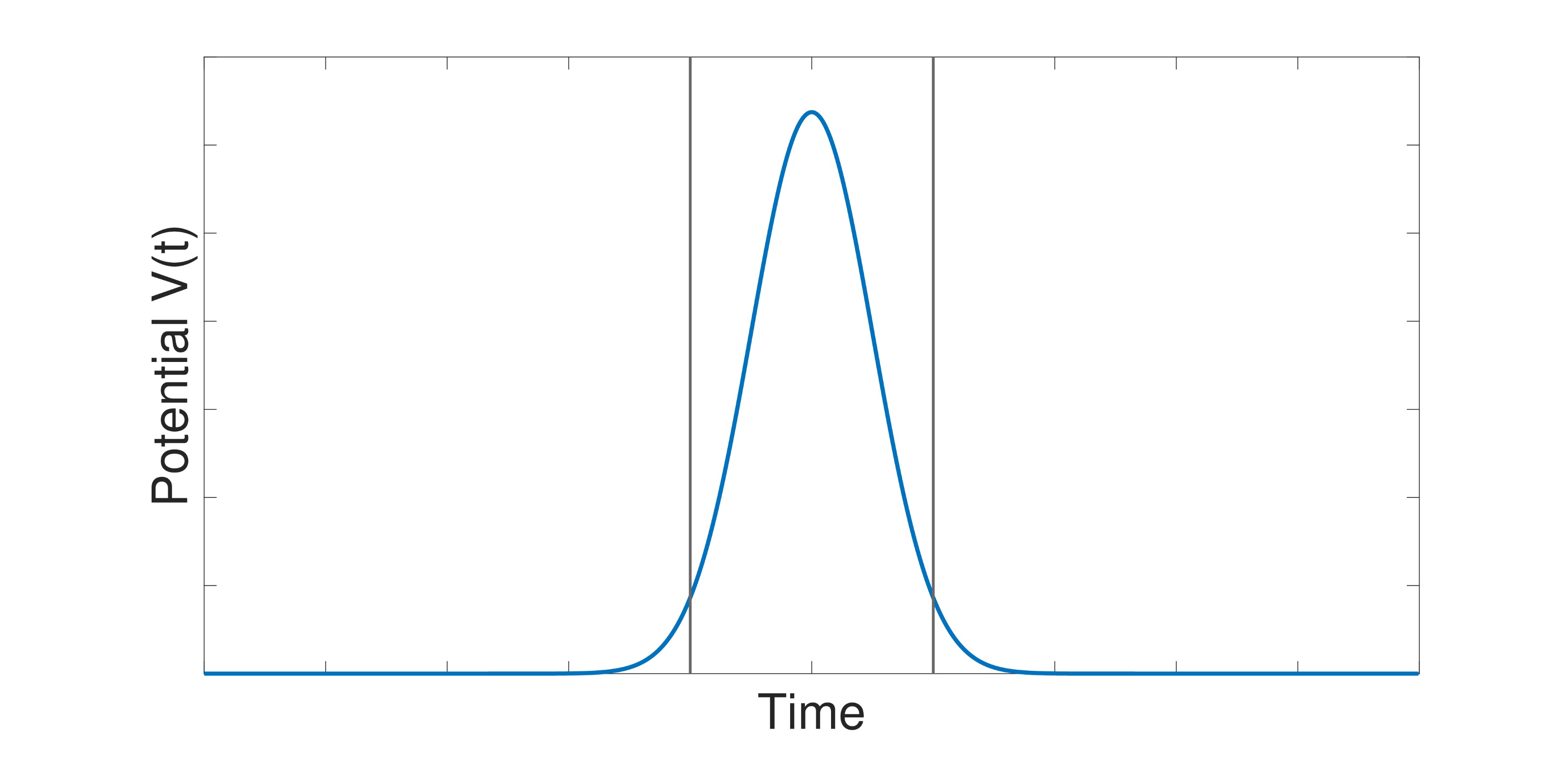
Figure 1: Experimental case: The Gaussian potential’s tails are truncated by the measurement. The integration windows for the TDSE are marked as vertical lines. The tails of the Gaussian are excluded, leading to Gibbs ringing in the frequency domain (not shown).

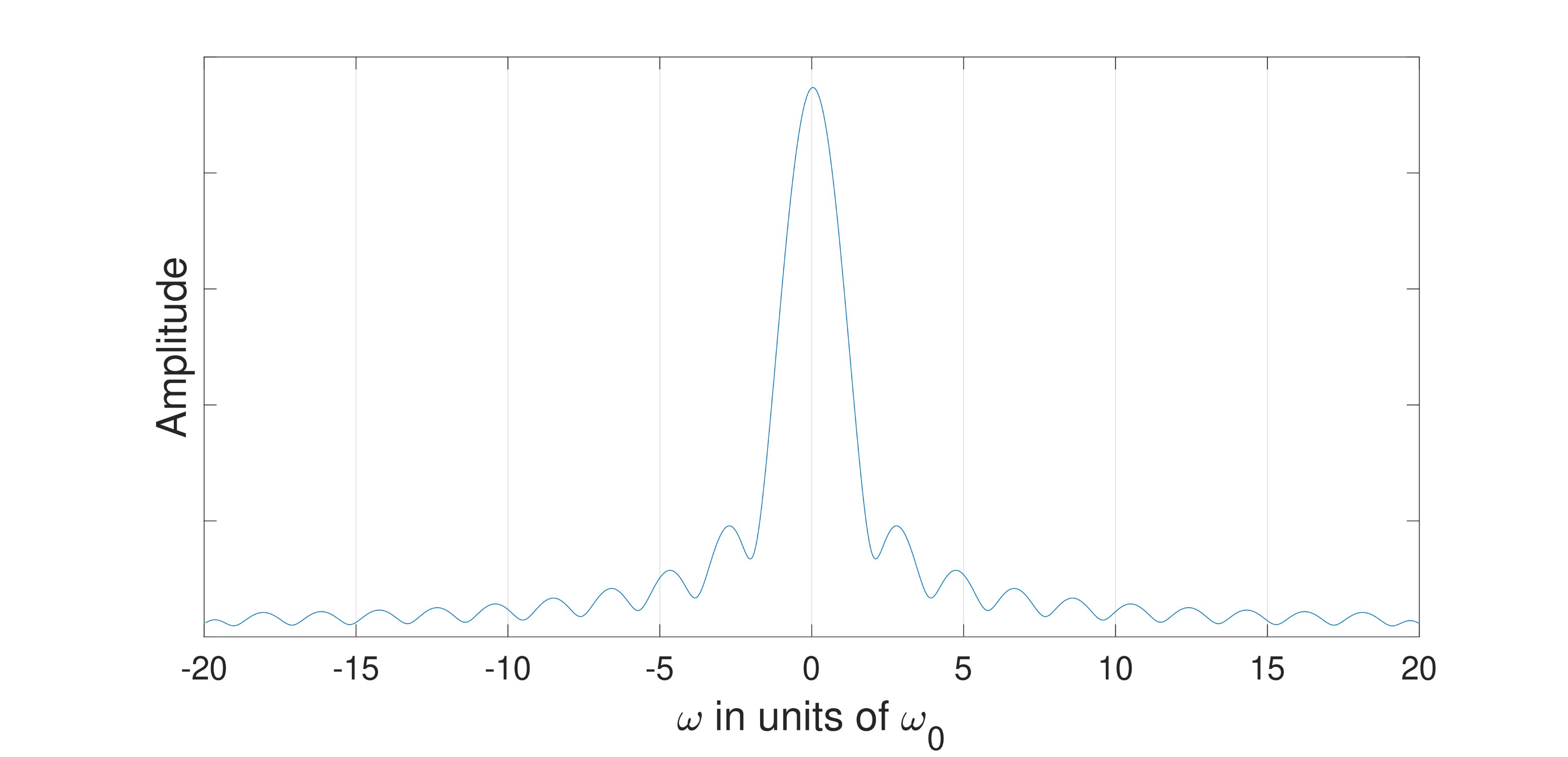
Figure 2: A Gaussian potential in $\omega$-space convolved with $sinc(\omega\Delta t)$ in Eq. 9.

II.2 Examples

Two standard cases will be considered to illustrate the validity of the result above.

II.2.1 Example: Fermi’s Golden Rule

It will first be verified that Eq. 9 reduces to the well-known Fermi Golden Rule. Consider the Hamiltonian for an oscillation perturbation potential:

$$\begin{split}\hat{H}&=\hat{H}_{0}\text{ for }t\leq 0\\ \hat{H}&=\hat{H}_{0}+\hat{V}(t)\text{ for }t>0\\ \hat{V}(t)&=2\hat{V}cos(\omega_{d}t)\end{split}$$ (10)

The standard integral in Eq. 5 results in the following coefficient for the $i\rightarrow f$ transition:

$$\begin{split}c_{f}^{(1)}(t)&=\frac{1}{i\hbar}\int_{0}^{t}dt_{1}e^{i(\omega_{f}-\omega_{i})t_{1}}(e^{i\omega_{d}t_{1}}+e^{-i\omega_{d}t_{1}})\braket{\omega_{f}}{\hat{V}}{\omega_{i}}\\ &=\frac{V_{fi}}{i\hbar}\left(\frac{e^{i(\omega_{fi}+\omega_{d})t}-1}{i(\omega_{fi}+\omega_{d})}+\frac{e^{i(\omega_{fi}-\omega_{d})t}-1}{i(\omega_{fi}-\omega_{d})}\right)\\ &\approx\frac{V_{fi}}{i\hbar}e^{i\frac{(\omega_{fi}-\omega_{d})}{2}t}\left(\frac{sin((\omega_{fi}-\omega_{d})t/2)}{(\omega_{fi}-\omega_{d})}\right),\end{split}$$ (11)

where $\omega_{fi}\equiv\omega_{f}-\omega_{i}$, and $t\rightarrow T$ is defined as a finite-time interval. We dropped the first term, as is customary, in favor of the second term, which dominates around the resonant frequency $\omega_{fi}=\omega_{d}$. [26]

Starting in a known state $c_{i}=1$ so the sum over $i$ can be dropped, then computing

$$\mathcal{F}\{V(t)\}\approx\frac{1}{2}\left(\delta(\omega-\omega_{d})+\delta(\omega+\omega_{d})\right)$$

but dropping the $+$ term as above, Eq. 8 gives

$$\begin{split}\tilde{\psi}^{(1)}(\omega_{f};T)&=\frac{1}{2\pi i\hbar}V_{fi}\,\Big{(}Te^{i\omega T/2}sinc(\omega T/2)\ast\delta(\omega-\omega_{d})\ast\delta{(\omega-\omega_{i})}\Big{)}\Big{|}_{\omega=\omega_{f}}\\ &=\frac{1}{2\pi i\hbar}V_{fi}\,Te^{i(\omega_{f}-\omega_{i}-\omega_{d})T/2}sinc((\omega_{f}-\omega_{i}-\omega_{d})T/2)\end{split}$$ (12)

which is the standard result (up to constant factors).

II.2.2 Example: Kicked harmonic oscillator

Another simple system to consider is the harmonic oscillator “kicked” by a small Gaussian pulse,

$$\begin{split}V(t)\propto e^{-\frac{t^{2}}{2\tau^{2}}},\end{split}$$ (13)

where $\tau$ is the characteristic time of the gaussian.

Using Eq. 5, the integral over a finite duration is typically extended to asymptotic time to become a Fourier transform, resulting in the approximate expression

$$\begin{split}c^{(1)}(t\rightarrow\infty)\propto\frac{\tau}{\sqrt{\omega_{(0)}}}e^{-\omega^{2}\tau^{2}/2},\end{split}$$ (14)

where $\omega_{(0)}$ is a normalization constant owing to the fixed natural frequency of the oscillator, and $\omega$ parameterizes the frequency response of the Gaussian perturbation.

Using instead Eq. 9, assuming that the initial oscillator is in a single $i$ energy eigenstate $\exp{(-i\omega_{i}\tau)}\ket{\omega_{i}}$ with certainty ($c_{i}=1$), an expression can be written for the amplitude associated with obtaining the $a$th energy eigenstate,

$$\begin{split}\,c^{(1)}(\omega_{a})=\frac{\tau}{2\pi i\hbar}V_{fi}\,\Big{(}e^{i\omega\tau/2}sinc(\omega\tau/2)\ast e^{-\omega^{2}\tau^{2}/2}\ast\delta(\omega-\omega_{i})\Big{)}\Big{|}_{\omega=\omega_{f}}\end{split}$$ (15)

Eqs. 14 and 15 convey similar information; however, Eq. 15 is exact. In Eq. 15, the normalization factor based on the oscillator frequency was incorporated into the definition of $V_{fi}$. Both equations include a linear factor for the time interval $\tau$. In the latter expression, the Gaussian dependence on $\omega$ is centered on the initial state, as expected for a kicked state, and is convolved with a phase shifted $sinc$ function. The effect of convolution is to add a small ripple to the Gaussian. (See Fig. 2) This ripple was ignored in the standard approach (Eq. 14), when the limits of integration are arbitrarily set to infinity.

III Decoupling TDSE through second-order RFT

Having examined the familiar first-order result using recursive Fourier transform methods, we now derive our second main result: an expression for the second-order term in the TDSE expansion.

The integrals for the second-order amplitudes are more complicated because the upper limit of integration for the nested integral is the integration parameter for the outer integral $t_{1}$. Starting from Eq. 4, by inserting a discrete basis of equally spaced states, the second-order transition amplitude is:

$$\begin{split}\tilde{\psi}^{(2)}(\omega_{f};T)=&\frac{1}{(i\hbar)^{2}}\sum_{ki}\int_{0}^{T}dt_{1}\int_{0}^{t_{1}}dt_{2}\bra{\omega_{f}}\hat{V}_{I}(t_{1})\ket{\omega_{k}}\bra{\omega_{k}}\hat{V}_{I}(t_{2})\ket{\omega_{i}}\tilde{c}_{i}(t=0)\\ =&\frac{1}{(i\hbar)^{2}}\int_{0}^{T}dt_{1}\Big{\{}e^{i\omega_{f}t_{1}}V(t_{1})\sum_{k}e^{-i\omega_{k}t_{1}}V_{fk}\\ &\qquad\qquad\qquad\int_{0}^{t_{1}}dt_{2}e^{i\omega_{k}t_{2}}V(t_{2})\sum_{i}e^{-i\omega_{i}t_{2}}V_{ki}\,\tilde{c}_{i}(t=0)\Big{\}}\end{split}$$ (16)

The integrals are therefore coupled, and the method in sec. II.1 must be modified. This is a Dyson series, and was decoupled by Dyson by introducing the time ordering operator. This is used widely in quantum field theory.[3]

Here the integrals will be decoupled in a new way in the following four steps.

Step 1.

Apply the convolution theorem to the nested integral

The limits of integration of the nested integral are extended to infinity, using a rectangular mask, as in Eq. 7,

$$\begin{split}\tilde{\psi}^{(2)}(\omega_{f};T)=&\frac{1}{(i\hbar)^{2}}\int_{0}^{T}dt_{1}e^{i\omega_{f}t_{1}}V(t_{1})\sum_{k}e^{-i\omega_{k}t_{1}}V_{fk}\\ &\,\Big{\{}\int_{-\infty}^{\infty}dt_{2}e^{i\omega_{k}t_{2}}rect\left(\frac{t_{2}}{\Delta t_{1}}-\frac{1}{2}\right)V(t_{2})\sum_{i}e^{-i\omega_{i}t_{2}}V_{ki}\,\tilde{c}_{i}(t=0)\Big{\}}\\ \end{split}$$ (17)

Because we truncated the signal using a $rect(t)$ mask, this step was exact. The integrals are still coupled via $\Delta t_{1}$, but the coupling now parameterizes the width of the mask rather than the integration domain.

By following the steps in Eq. 7, we can write each factor in the integrand of the second line of Eq. 17 in the frequency domain.

$$\begin{split}\tilde{\psi}^{(2)}=&\frac{1}{2\pi(i\hbar)^{2}}\int_{0}^{T}dt_{1}e^{i\omega_{f}t_{1}}V(t_{1})\sum_{ki}e^{-i\omega_{k}t_{1}}V_{fk}V_{ki}\tilde{c}_{i}(t=0)\\ &\underset{t_{2}\rightarrow\omega_{k}}{\mathcal{F}}\Big{\{}\underset{\omega\rightarrow t_{2}}{\mathcal{F}^{-1}}\{\Delta t_{1}\exp{(i\omega\Delta t_{1}/2)}sinc(\omega\Delta t_{1}/2)\cdot\underset{\omega\rightarrow t_{2}}{\mathcal{F}^{-1}}\{\tilde{V}(\omega)\}\underset{\omega\rightarrow t_{2}}{\mathcal{F}^{-1}}\{\delta(\omega-\omega_{i})\}\Big{\}}\end{split}$$ (18)

and apply the convolution theorem,

$$\begin{split}\tilde{\psi}^{(2)}=&\frac{1}{2\pi(i\hbar)^{2}}\int_{0}^{T}dt_{1}e^{i\omega_{f}t_{1}}V(t_{1})\sum_{ki}e^{-i\omega_{k}t_{1}}V_{fk}V_{ki}\tilde{c}_{i}(t=0)\\ &\qquad\left(\Delta t_{1}e^{i(\omega-\omega_{i})\Delta t_{1}/2}sinc((\omega-\omega_{i})\Delta t_{1}/2)\ast\tilde{V}(\omega)\right)\Big{|}_{\omega=\omega_{k}}\end{split}$$ (19)

In evaluating the Fourier transforms, we have transformed bases from the original parameter of integration, $\omega$, to $t_{2}$ and then to $\omega_{k}$, an intermediate basis of energy states. Note that the expression inside the parenthesis on the last line of Eq. 19 is a continuous distribution in a dummy parameter $\omega$, evaluated at a specific value $\omega=\omega_{k}$ after performing the convolution.

The nested integral is now a convolution in $\omega$-space, but the $sinc$ function’s width depends on $t_{1}$, which is coupled to the outer integral. How do we compute a convolution of a signal whose shape is changing as $t_{1}$ is integrated over?

Step 2.

Discretize the integral over $\Delta t_{1}$ as a Riemann sum and move it inside the sum over $k$ and $i$

It is easier to handle Eq. 19 by writing the integral over $\Delta t_{1}$ as a Riemann sum of step size $T$, and rearranging the sums:

$$\begin{split}\tilde{\psi}^{(2)}=&\frac{1}{2\pi(i\hbar)^{2}}\sum_{ki}V_{fk}V_{ki}\tilde{c}_{i}(t=0)\sum_{n=n_{i}}^{n_{f}}T\,e^{i\omega_{f}nT}V(nT)e^{-i\omega_{k}nT}\\ &\qquad\Big{(}nT\exp{(i(\omega-\omega_{i})nT/2)}sinc((\omega-\omega_{i})nT/2)\ast\tilde{V}(\omega)\Big{)}\Big{|}_{\omega=\omega_{k}}\end{split}$$ (20)

Because the second line is a distribution in $\omega$ evaluated at a specific point, it is simply a c-number for each term in the Riemann sum.

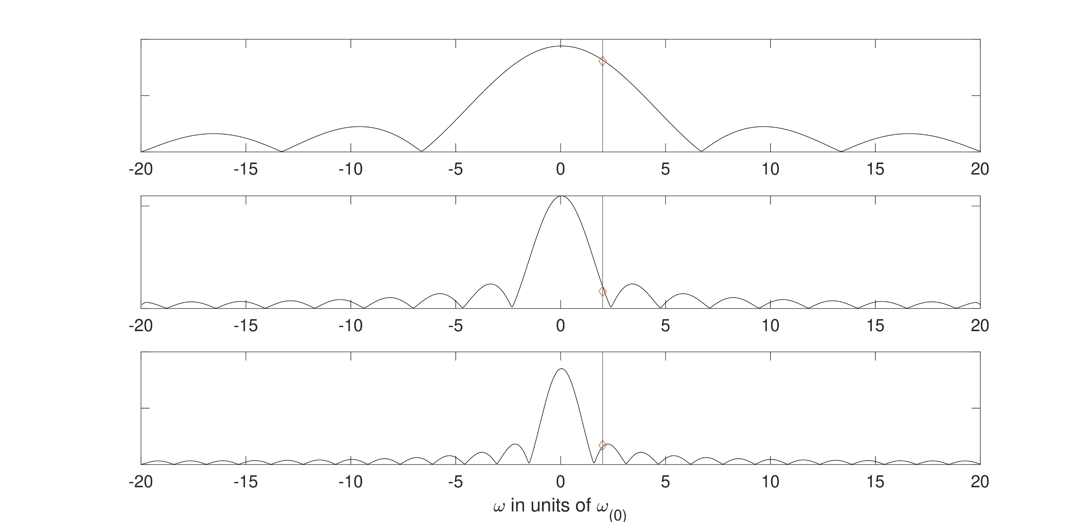
Figure 3: The width of the $sinc$ function depends on $\Delta t_{1}$. In the figure, $\Delta t_{1}$ increase from top to bottom. While varying the $sinc$ over $\Delta t_{1}$ we take samples at $\omega_{k}$ (diamond on vertical line). The sample values trace out another $sinc$ function.

Step 3.

Allow the variation over time to vary the width of the distributions $sinc(\omega\Delta t_{1})$

Here is the central insight to decouple the integrals. For each step in the Riemann sum over $n$ (coupling variable), the impulse response is defined as:

$$\begin{split}\boxed{h_{ki}[\Delta t_{1}]\equiv\Big{(}\exp{(i(\omega-\omega_{i})\Delta t_{1}/2)}\frac{sin((\omega-\omega_{i})\Delta t_{1}/2)}{(\omega-\omega_{i})/2}\ast\tilde{V}(\omega_{f})\Big{)}\Big{|}_{\omega=\omega_{k}}}\end{split}$$ (21)

where $\Delta t_{1}=nT$. Eq. 21 can be seen as an impulse response of the system to a perturbation of duration $\Delta t_{1}$. Eq. 21 is the second line of Eq. 20 (see fig. 4).

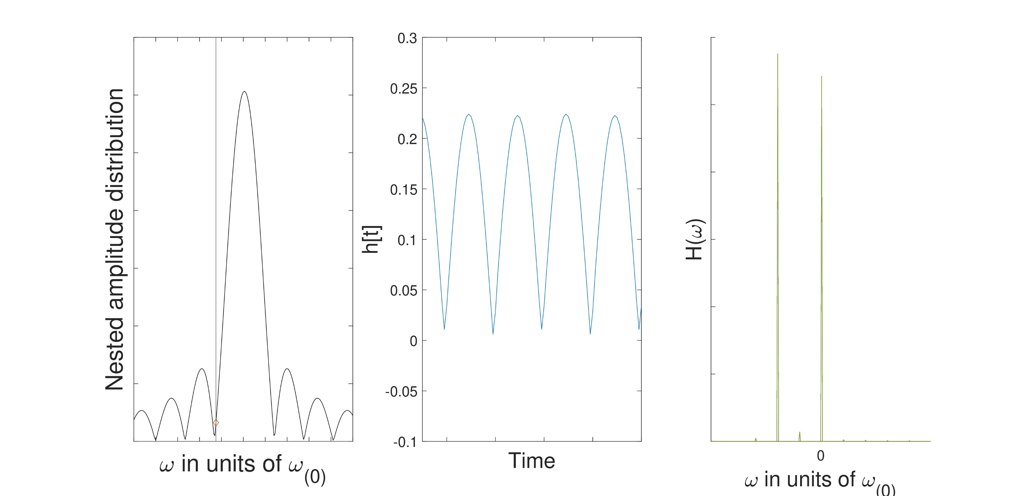
Figure 4: (Left) Nested $sinc$ distribution (second line in Eq. 19), varied in width over $\Delta t_{1}$, while repeatedly sampled at $\omega_{k}=-2\omega_{(0)}$ (vertical line). As the width of the $sinc$ decreases its height grows due to the linear factor of $\Delta t_{1}$. (Middle) The samples oscillate ($h_{ki}[\Delta t]$) as $\Delta t$ is varied. (Right) The Fourier transform $\tilde{H}_{ki}(\omega)=\mathcal{F}\{h_{ki}[\Delta t]\}$ is a series of spikes representing second-order impulses. These $\delta$-functions are convolved in Eq. 24 to place a copy of the outer $sinc$ at each impulse.

Step 4.

Apply the convolution theorem to the outer integral

Now we can change the Riemann sum back to an integral over $\Delta t_{1}$. Crucially, $h_{ki}$, which is an explicit distribution in $\omega$-space, appears inside an integral over time $\Delta t_{1}$, we interpret it as a function of time rather than frequency. We can now repeat the earlier technique of extending the integration domain in the first-order to $\pm\infty$ and inserting a rectangular function of width $T$,

$$\begin{split}\tilde{\psi}^{(2)}=&\frac{1}{2\pi(i\hbar)^{2}}\sum_{ki}V_{fk}V_{ki}\tilde{c}_{i}(t=0)\int_{-\infty}^{\infty}dt_{1}e^{i\omega_{f}\Delta t_{1}}rect\left(\frac{t_{1}}{T}-\frac{1}{2}\right)V(t_{1})e^{-i\omega_{k}\Delta t_{1}}h_{ki}[t_{1}].\end{split}$$ (22)

The effect of the outer integral over $t_{1}$ on the nested integral is to vary the width $t_{1}$ (or more precisely $\Delta t_{1}$) of the impulse response across the duration of the measurement window from $0\rightarrow T$, and sample it at $\omega_{k}$ to generate $h_{ki}[\Delta t_{1}]$ (see fig. 3).

Because of Step 3, everything inside the $t_{1}$ integral in Eq. 22 can be treated as a distribution in $t_{1}$, and the convolution theorem can be used again. The $t_{1}$ integral becomes a Fourier transform by explicitly writing each factor in the $\omega$-domain,

$$\begin{split}\underset{t_{1}\rightarrow\omega_{f}}{\mathcal{F}}\Bigg{\{}\underset{\omega\rightarrow t_{1}}{\mathcal{F}^{-1}}\Big{\{}Te^{i\omega T/2}sinc(\omega T/2)\Big{\}}\cdot\underset{\omega\rightarrow t_{1}}{\mathcal{F}^{-1}}\Big{\{}\tilde{V}(\omega)\Big{\}}\underset{\omega\rightarrow t_{1}}{\mathcal{F}^{-1}}\Big{\{}\delta(\omega-\omega_{k})\Big{\}}\cdot\underset{\omega\rightarrow t_{1}}{\mathcal{F}^{-1}}\Big{\{}\tilde{H}_{ki}(\omega)\Big{\}}\Bigg{\}},\end{split}$$ (23)

where $\tilde{H}_{ki}(\omega_{k},\omega_{i})\equiv\mathcal{F}\{h_{ki}[t_{1}]\}$ is the Fourier transform of the impulse response, which is also called the amplitude transfer function.

The final $\omega$-domain expression for second-order transition amplitude from $n\rightarrow a$ is

$$\begin{split}\boxed{\tilde{\psi}^{(2)}(\omega_{f};T)=\sum_{ki}c_{bn}\Bigg{\{}Te^{i\omega_{f}T/2}sinc\left(\frac{\omega_{f}T}{2}\right)\ast\tilde{V}(\omega_{f})\ast\delta(\omega_{f}-\omega_{k})\ast\tilde{H}_{ki}(\omega_{f})\Bigg{\}}}\end{split}$$ (24)

where

$$\begin{split}\boxed{\tilde{H}_{ki}(\omega)=\underset{\Delta t_{1}\rightarrow\omega}{\mathcal{F}}\Big{\{}\Big{(}\exp{(i(\omega^{\prime}-\omega_{i})\Delta t_{1}/2)}\frac{sin((\omega^{\prime}-\omega_{i})\Delta t_{1}/2)}{(\omega^{\prime}-\omega_{i})/2}\ast\tilde{V}(\omega^{\prime})\Big{)}\Big{|}_{\omega^{\prime}=\omega_{k}}\Big{\}}}\end{split}$$ (25)

For notational simplicity we have defined $c_{ki}\equiv c_{i}V_{fk}V_{ki}/(2\pi i\hbar)^{2}$.

This is the second main result, expressing the second-order contribution to the transition amplitude owing to the time-limited perturbation of an arbitrary system with energy eigenfunctions $\psi_{n}$.

We assume that the spectra of the energy eigenstates $\omega_{k}$ and $\omega_{i}$, are discrete. For simplicity, we consider only the case in which they are equally spaced, that is, a simple harmonic oscillator. Then we can write $\omega_{ki}=k\omega_{(0)}$. See fig. 5.

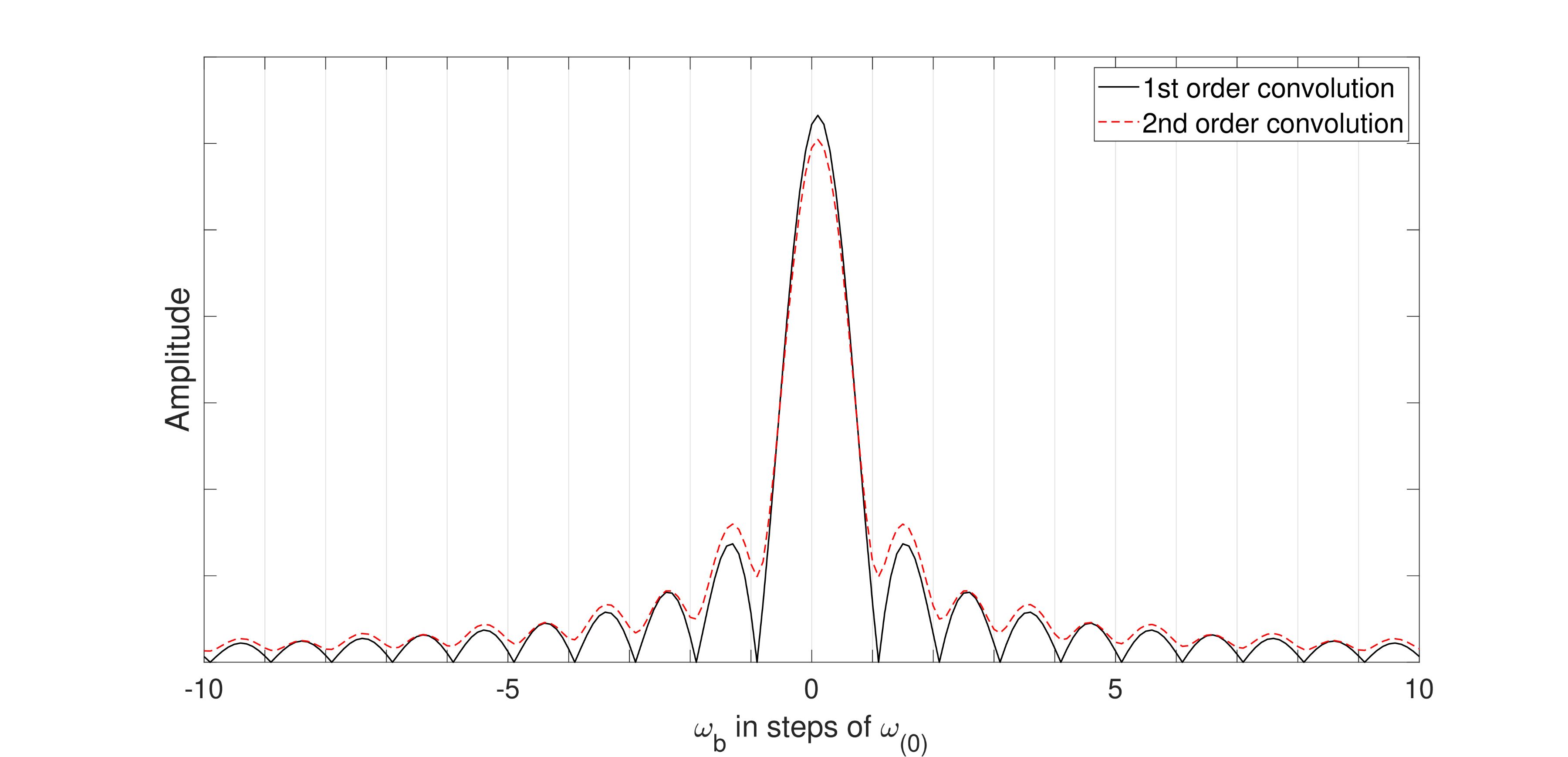
Figure 5: Comparison of first and second-order convolution for a system in an initial state $\omega_{i}=0$. The second-order calculation computes paths through intermediate energies at $\pm 20\omega_{(0)}$. For the second-order calculation, the central peak is reduced, the wings are amplified, and the minima are increased. Only the range $\pm 10\omega_{(0)}$ is shown, but the contributions from terms outside this range have a significant effect on the accuracy of the result.

IV Functional analysis

We will now examine Eqs. 24 and 25 in more detail.

IV.1 The transfer function

Evaluating the form of the transfer function $\tilde{H}_{ki}$ can be performed first for the case of a negligible potential, $\tilde{V}(\omega_{f})=\delta(\omega)$ (infinitely wide in the time domain). Because convolution with a $\delta$-function is the identity operation, we can then evaluate $h_{ki}[t]$ explicitly and take its Fourier transform,

$$\begin{split}\tilde{H}_{ki}&=\underset{\Delta t_{1}\rightarrow\omega}{\mathcal{F}}\Big{\{}\exp{(i\omega_{ki}\Delta t_{1}/2)}\frac{sin(\omega_{ki}\Delta t_{1}/2)}{\omega_{ki}/2}\Big{\}}\\ &=\frac{2\pi i}{\omega_{ki}}\left(\delta(\omega+\omega_{ki}/2+\omega_{ki}/2)-\delta(\omega-\omega_{ki}/2+\omega_{ki}/2)\right)\\ &=\frac{2\pi i}{\omega_{ki}}\left(\delta(\omega+\omega_{ki})-\delta(\omega)\right).\end{split}$$ (26)

In other words, the transfer function is composed of a series of discrete impulses spaced at integer multiples of $\omega_{(0)}$ (because $\omega_{ki}=k\omega_{(0)}$). See fig. 4.

Next $\tilde{H}_{ki}$ is convolved with the other factors in Eq. 25, resulting in

$$\begin{split}\delta(\omega-\omega_{k})\ast\tilde{H}_{ki}&=\frac{2\pi i}{\omega_{ki}}\delta(\omega-\omega_{k})\ast\left(\delta(\omega+\omega_{ki})-\delta(\omega)\right)\\ &=\frac{2\pi i}{\omega_{ki}}\left(\delta(\omega-\omega_{i})-\delta(\omega-\omega_{k})\right)\end{split}$$ (27)

As shown in figs. 6 and 7, each term in the sum over $b$ contributes complex impulses at $\omega_{k}$ and $\omega_{i}$. From top to bottom the cases $k=-1,0,1$ are graphed consecutively, with $i=0$. (imaginary portion is solid, real portion is dashed.) The top and bottom graphs correspond to Eq. 26.

The special case $k=i$ must be handled separately. Here, the desirable properties of the $sinc$ function at the origin are required, and Eq. 26 is the Fourier transform of a constant:

$$\begin{split}\tilde{H}_{00}&=\mathcal{F}\Big{\{}\text{constant}\Big{\}}=2\pi\delta(\omega).\end{split}$$ (28)

This contributed to a purely real amplitude at the origin, as shown in the middle graph of fig. 6.

Summing over all $\tilde{H}_{ki}$ contributions over the range $k=\pm 25$, it can be seen in fig. 8 that for $k\neq 0$, $\tilde{H}_{ki}$ contributes a real portion at $\omega_{k}=0$ which is amplified as more frequencies are included ($k\rightarrow\pm\infty$) whereas the real portion remains small and finite at every other $\omega_{k}$, vanishing when the distribution is normalized (top). Conversely, the imaginary portions cancel at $\omega_{k}=0$ but are significant everywhere else, decaying inversely with respect to $|k|$ (middle).

An analogy can be drawn to the frequency-domain decomposition of sound signals. In the second-order calculation, the probability amplitude signal was deflected into a series of higher harmonics. Similarly, an acoustic musical instrument generates sound through the combination of a pluck (impulse) and resonant cavity that amplifies higher harmonics (impulse response). This is similar to the relationship between $\tilde{H}_{ki}$ in Eq. 24 and the rest of that equation.

IV.2 Stepping through the algorithm for transfer function

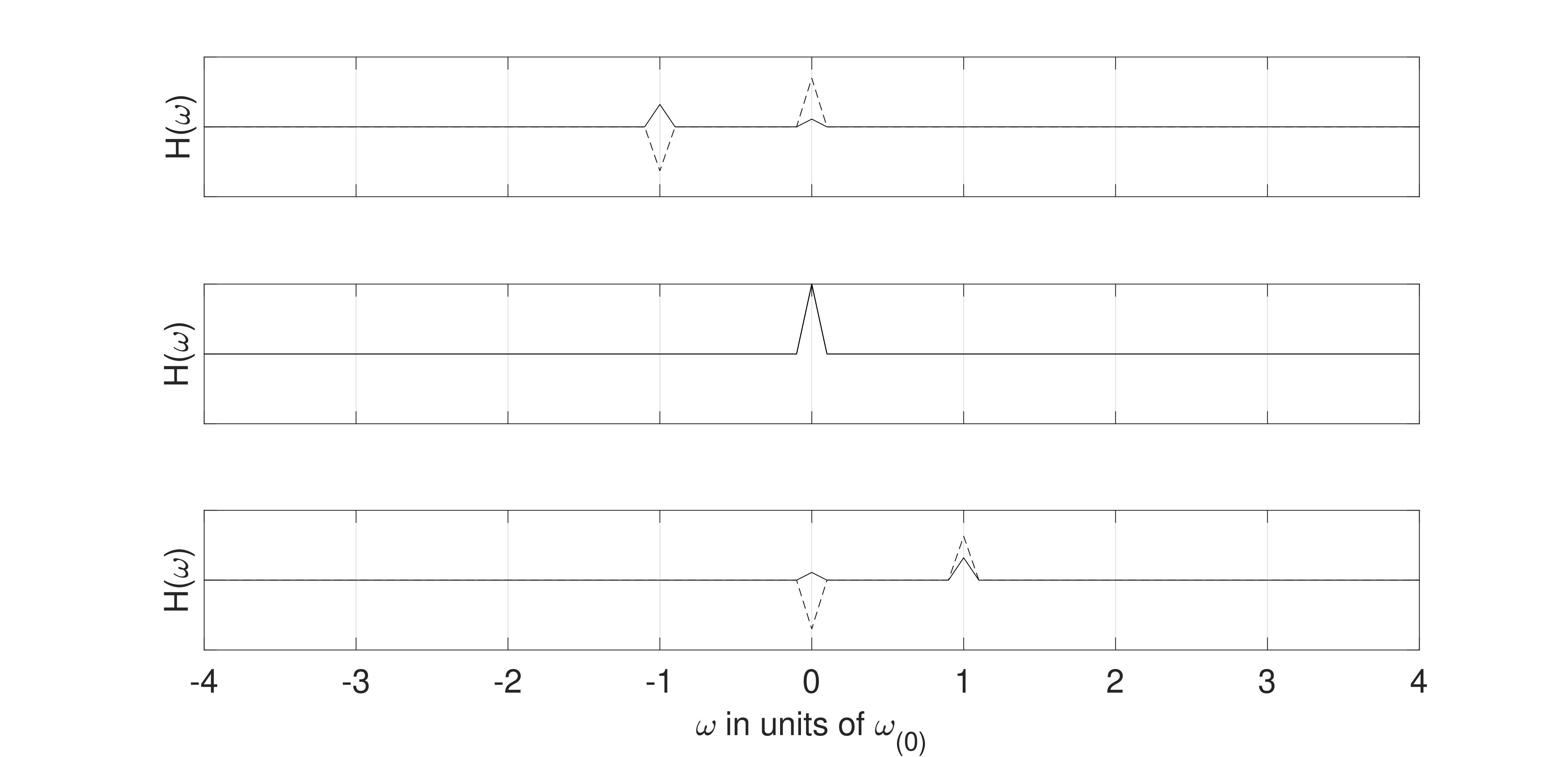
Figure 6: Contributions to the second-order complex valued “transfer function” $\tilde{H}_{ki}$ from the frequencies $k=-1,0,1$. The cases $k=\pm 1$ contribute a real portion (solid) and an imaginary portion (dashed) at $\omega_{k}=\pm 1$. The case $k=0$ contributes only a real portion (solid). See Eq. 26 and 28.

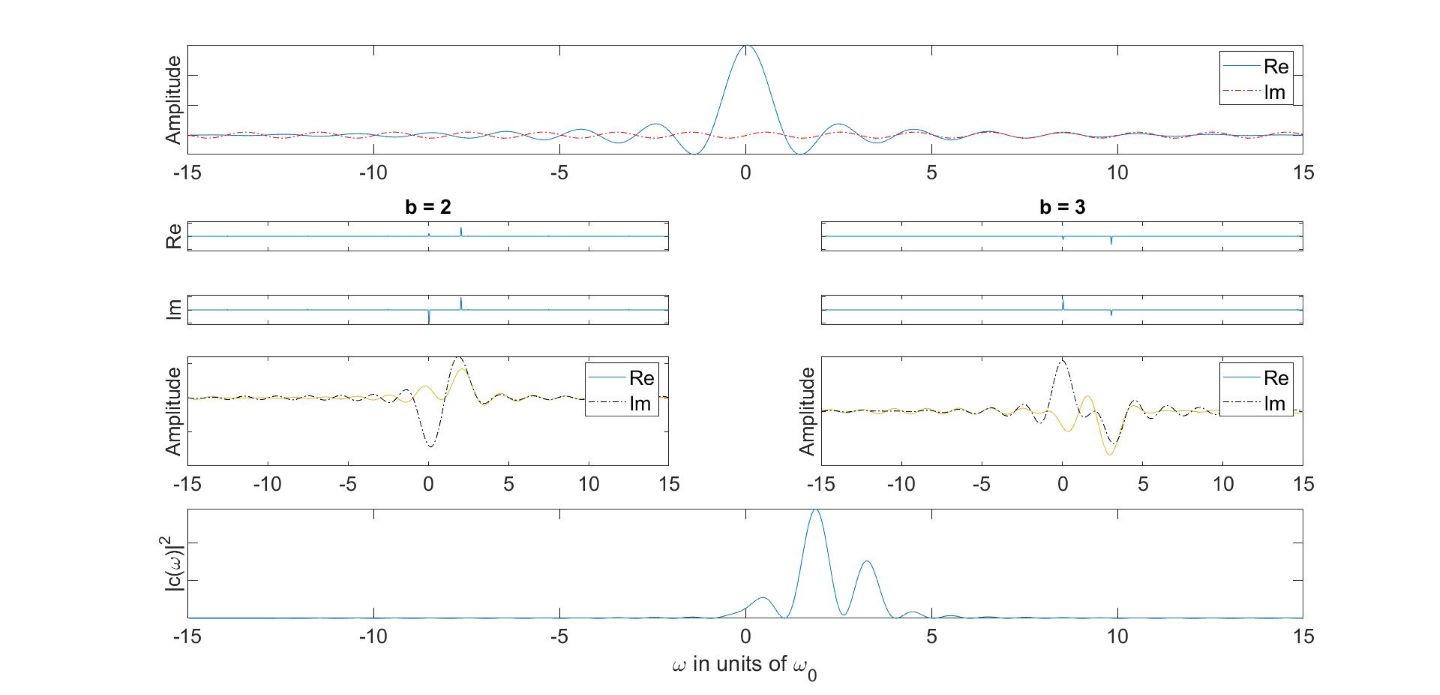
Figure 7: The frequency-distributions for $k=2,3$ contributions. (Top) The real (solid) and imaginary (dashed) parts of the complex $sinc$ function in Eq. 24, corresponding to the outer integral over $t_{1}$ in Eq. 19. (2nd/3rd row) The transfer function $\tilde{H}_{ki}(\omega)$ in Eq. 25 captures information from the nested $t_{2}$ integral as a series of spikes, $\delta(\omega-2\omega_{(0)})+\delta(\omega)$, (left), $\delta(\omega-3\omega_{(0)})+\delta(\omega)$, (right). See Eq. 26. (4th row) The real (solid) and imaginary (dashed) parts of the convolution in Eq. 24. (Bottom) The combined result from $k=2$ and $k=3$.

A comparison was made between the direct integration of Eq. 4 and the convolution approach in Eqs. 24 and 25 using MATLAB. The program begins by generating a nested impulse response, Eq. 21. This has the form $sinc\ast V$ and width $\Delta t_{1}$, as shows in Fig. 4 (far-left).

This impulse response (in $\omega$) is then varied over time across the integration limits $0<\Delta t_{1}<T$, generating a sequence of $sinc$ graphs of varying widths. The sample value at the vertical line $\omega_{k}$ for each graph was stored as a new array $h_{ki}[\Delta t]$ (Fig. 4, middle). For a given $\omega_{k}$, these samples oscillate with a frequency profile that is dependent on the physics of the experiment (such as the properties of the potential and duration of the window of measurement).

The Fourier transform of $h_{ki}[\Delta t]$ is $\tilde{H}_{ki}(\omega)$ (fig. 4 right panel). It is a series of impulses representing each intermediate contribution to the second-order amplitude (see figs. 6 and 8). If the perturbation is negligible, we can write $\tilde{V}(\omega)=\delta(\omega)$. In this case $\tilde{H}_{ki}$ is composed of $\delta$-function impulses at $\omega_{k}$ and $\omega_{i}$. If the potential is strong, other harmonics appear in this graph (see fig. 9 bottom-right).

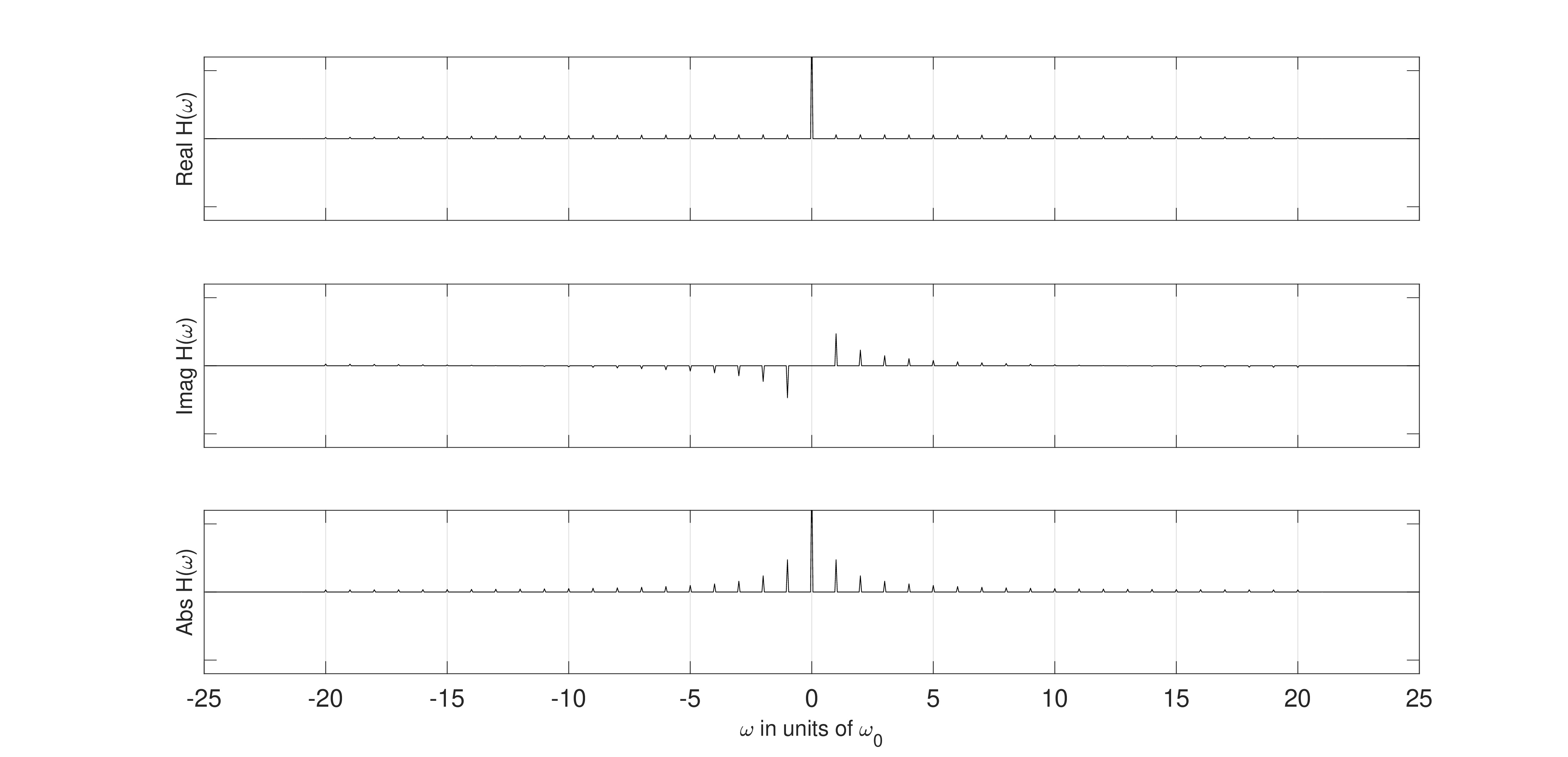
Figure 8: $\tilde{H}_{ki}(\omega)$ for $-25<b<25$. The contribution to $\tilde{H}_{ki}(\omega)$ at $k=0$ is non-zero for every $b\neq 0$, growing without bound, as we include more momenta ($b\rightarrow\infty$), see Eq. 28. There is also a small, constant, real contribution at each $\omega_{k}$, vanishes when the distribution is normalized (top). The imaginary portions cancel at $\omega_{k}=0$ and are built everywhere else, decaying inversely to $|b|$ (middle), see Eq. 26. The absolute magnitude of $\tilde{H}_{ki}$ was a harmonic series of impulses (bottom). These impulses are convolved with the first-order impulse response, Eq. 9.

Finally, in Eq. 24, $\tilde{H}_{ki}$ is convolved with a phase-shifted $sinc$ impulse response so that a copy of the impulse response is placed wherever $\tilde{H}_{ki}$ has a spike, as shown in Fig. 7. This is performed for every possible intermediate state $\omega_{k}$, and the amplitude plots for each are summed. Each code loop over $\omega_{k}$ contributes an impulse response centered at $\omega_{k}$ and another centered at $\omega_{i}$ (fig. 6).

After looping over all $2b+1$ intermediate distributions, the impulses centered on $\omega_{i}$ reinforce $2b+1$ times, whereas the second-order signal at each $\omega_{k}$ appears only once. The result is a strong central peak, and decaying wings (fig. 5).

IV.3 Domain and resolution of transfer function

In the code implementation of Eq. 21, the length of $h_{ki}[\Delta t_{1}]$ is not equal to the length of the original signal. This is because $h_{ki}[\Delta t_{1}]$ is generated by scanning $\Delta t_{2}$ over the variable range $0<\Delta t_{2}<t_{1}$. Thus, the corresponding resolution of its Fourier transform, $\tilde{H}_{ki}$, is reduced (fig. 9, top left).

To compensate for the band-limited spectrum, $\tilde{H}_{ki}$ was padded with copies of itself. This is necessary for the convolution operation to be well-defined. The time window $T$ was chosen to be an integer fraction of the duration of the original signal so that the padding fits evenly (this is necessary to avoid artifacts in the Fourier transform).

This defines a fundamental harmonic frequency associated with the measurement,

$$\begin{split}\omega_{(1)}&\equiv\text{total duration of original signal}/\text{duration of time integration}\\ &=\frac{1}{T},\end{split}$$ (29)

(see the harmonic spacing in Fig. 8).

When the Gaussian potential is weak, the tiled instances of $h_{ki}[\Delta t_{1}]$ line up smoothly, and $\tilde{H}_{ki}$ only contains two spikes, as in Eq. 26 and fig. 6. When the potential is stronger, $h_{ki}[\Delta t_{1}]$ does not line up on its endpoints, and spectral artifacts occur at integer multiples of $\omega_{(1)}$.

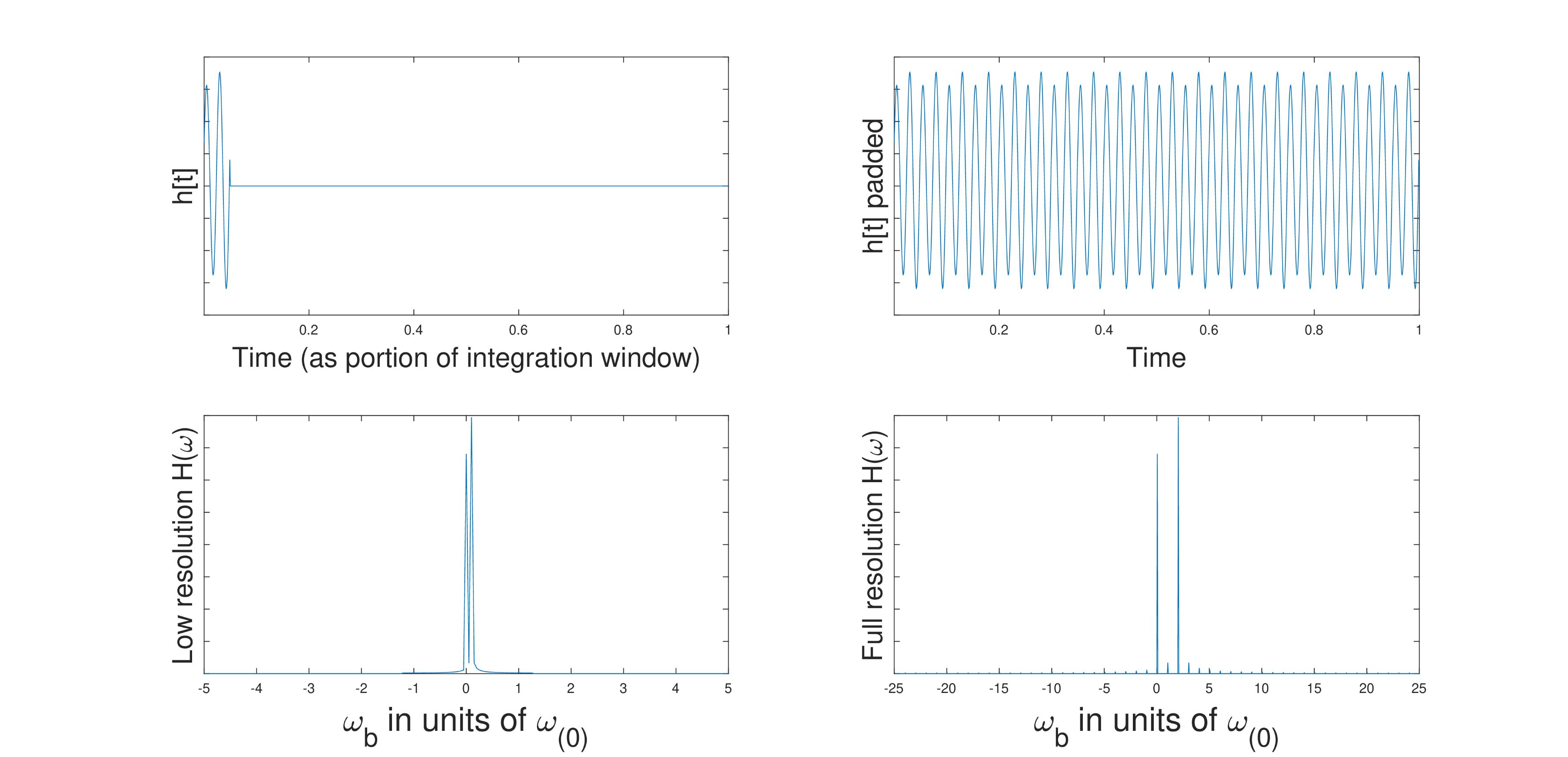
Figure 9: Bandlimited signal: Because the duration of the time integration of the TDSE is less than the full signal (5% shown here, top left), $h_{ki}[t]$ is smaller than $\tilde{V}$ by that factor, and the resolution is decreased (lower left, the distinct spikes are only resolvable because horizontal scale is expanded). In the upper right, $h_{ki}[t]$ was padded with copies of itself (upper right) to compensate for the limited bandwidth of the signal. This ensures its Fourier transform has the desired high resolution (lower right). Shown here is the $k=+2$ term of Eq. 25. A moderate strength potential was used, resulting in harmonics at nearby states (see small spikes at $k=+1,+3$ and other integers in bottom right).

For reasons that are not fully understood by the author, the interpretation of the second-order results is clear only when $\omega_{(1)}=\omega_{(0)}$, which is known as cyclotron resonance. This appears to be related to the interpretation of Eqs. 24 and 25 as a signal reconstruction problem using sinc-interpolation: This is the only case considered in this study.

IV.4 Effect of time window shift on the form of the transfer function

In Fig. 8, the imaginary part of $\tilde{H}_{ki}$ decays inversely with $|b|$. The time measurement window was shown to extend from the origin to $\Delta t$, leading to a translational factor of $\frac{1}{2}$ in the $rect(t)$ function. In the general case, the measurement window can be translated $r$ units by shifting the $rect(t)$ function again, $rect(\frac{t}{\Delta t}-\frac{1}{2}-\frac{r}{\Delta t})$, leading to an overall phase shift in the frequency domain, $\exp{(i\omega_{k}(r/\Delta t))}$. This leads to an oscillating envelope for the impulses, as shown in Fig. 8 (not shown). In the MATLAB simulation a phase shift of this sort was introduced to compensate for coding artifacts (the base index for the time window started at 1 instead of 0).

IV.5 Normalizability

The appearance of $\omega_{ki}$ in the denominator of Eq. 21 inside summation over both $i$ and $k$ is the cause for questioning whether this expression can be normalized. However, owing to the good properties of the $sinc$ function, $h_{ki}$ and $\tilde{H}_{ki}$ are non-singular.

To observe this, note that when $1/\omega_{ki}$ becomes singular, we use Eq. 28 (which is well-defined) instead of Eq. 26.

In general, $\tilde{H}_{ki}$ is a series of harmonics of spacing $\omega_{(0)}$, as shown in Fig. 8. The middle plot shows imaginary impulses at every non-zero integer $\omega_{k}$ that form a harmonic series, which is well-known to not converge: therefore it is not clear whether the final expression eqn, 24 is convergent. The upper plot shows an impulse at $w_{i}=0$ resulting from each term in the sum over $b$. The height of this impulse increases without bounds for $b\rightarrow\pm\infty$. This is ultraviolet divergence.

This can easily be resolved from a practical perspective. Because the height of the impulse at the origin is proportional to the size of the domain, $|b_{max}|$, in the code implementation, this expression can be normalized by dividing by the maximum value of $b$, where only a finite number of terms are included.

From a theoretical perspective regarding the convergence of the second-order, the issue is whether the $sinc$ functions, each of which are normalizable and arranged in a harmonic series (which does not converge) are normalizable. This was not addressed in this study.

IV.6 Example: Second-order harmonic perturbation Golden Rule

To illustrate the results of Section III we compare the recursive Fourier transform method with the standard approach in the second-order.

Consider the ramped up oscillating potential,

$$V(t)=e^{\epsilon t}e^{-i\omega_{d}t},$$ (30)

where $\epsilon$ is a small constant which ensures ramp up of the potential from $t=-\infty$, and $\omega_{d}$ is the driving frequency of the potential.

Via traditional application of the TDSE to second-order, we integrate twice to obtain

$$c_{f}(t) =\left(-\frac{i}{\hbar}\right)^{2}\frac{e^{i(\omega_{fi}-2\omega_{d})t}e^{2\epsilon t}}{\omega_{fi}-2\omega_{d}-2i\epsilon}\sum_{k}\frac{V_{fk}V_{ki}}{\omega_{k}-\omega_{i}-\omega_{d}-i\epsilon}.$$ (31)

Taking the rate of the squared amplitude in the small $\epsilon$ limit results in

$$\begin{split}\lim_{\epsilon\to 0}\frac{d}{dt}|c_{f}(t)|^{2}\propto\Big{|}\sum_{k}\frac{V_{fk}V_{ki}}{\omega_{k}-\omega_{i}-\omega_{d}-i\epsilon}\Big{|}^{2}\delta(\omega_{f}-\omega_{i}-2\omega_{d})\end{split}$$ (32)

where the $\delta$-function comes from the small $\epsilon$ limit of

$$\lim_{\epsilon\to 0}\frac{2\epsilon}{(\omega_{fi}-2\omega_{d})^{2}+\epsilon^{2}}\Rightarrow\delta(\omega_{fi}-2\omega_{d})$$ (33)

Alternatively, using Eqs. 24 and 25 (to find the probability amplitude rather than the probability),

$$\begin{split}c_{f}(\omega_{f},t)\propto\sum_{k}V_{fk}V_{ki}te^{i(\omega_{f}-\omega_{i})t/2}sinc((\omega_{f}-\omega_{i})t/2)\ast\tilde{V}(\omega_{f})\ast\delta(\omega_{f}-\omega_{i})\ast\tilde{H}_{ki}(\omega_{f}),\end{split}$$ (34)

where

$$\begin{split}\tilde{H}_{ki}(\omega_{f})=\underset{t_{1}\rightarrow\omega_{f}}{\mathcal{F}}\Big{\{}\frac{e^{i(\omega^{\prime}-\omega_{i})\frac{t_{1}}{2}}sin((\omega^{\prime}-\omega_{i})\frac{t_{1}}{2})}{(\omega^{\prime}-\omega_{i})/2}\ast\tilde{V}(\omega^{\prime})\Big{|}_{\omega^{\prime}\rightarrow\omega_{k}}\Big{\}}\end{split}$$ (35)

Again this simplifies. At the limit of small $\epsilon$, the Fourier transform of the potential (Eq. 30) is the same as that in Eq. 33, in which case Eq. 26 and 28 can be used to obtain the transfer function,

$$\begin{split}\tilde{H}_{ki}(\omega_{f})\propto\frac{1}{(\omega_{k}-\omega_{i}-\omega_{d})/2}\left(\delta(\omega_{f}+(\omega_{k}-\omega_{i}-\omega_{d}))-\delta(\omega_{f})\right).\end{split}$$ (36)

Plugging into Eq. 34 obtains

$$\begin{split}c_{f}(\omega,t)\propto t\sum_{k}\frac{i}{\omega_{k}-\omega_{i}-\omega_{d}}\Big{(}&e^{i(\omega_{fi}-2\omega_{d})\frac{t}{2}}sinc((\omega_{fi}-2\omega_{d})\frac{t}{2})\\ &-e^{i(\omega_{f}-\omega_{i}-\omega_{d})\frac{t}{2}}sinc((\omega_{f}-\omega_{i}-\omega_{d})\frac{t}{2})\Big{)}.\end{split}$$ (37)

In the limit of small $\epsilon$ and small $t$, the prefactor denominator matches Eq. 32, and the first term inside the parentheses reduces to $\delta(\omega_{fi}-2\omega_{d})$, which is again consistent with Eq. 32. The second term inside the parenthesis peaks at $\omega_{f}-\omega_{i}=\omega_{d}$ whereas the prefactor peaks at $\omega_{k}-\omega_{i}=\omega_{d}$, so that the only non-zero contribution occurs when $\omega_{fi}=2\omega_{i}$.

Summing over $k$ gives $k$ peaks located at $\omega_{fi}=2\omega_{d}$ (combining to form one very high peak), plus one peak for each $k$ at $\omega_{fn}=\omega_{d}$ (a discrete series of small peaks, decaying in height as $\omega_{i}-\omega_{i}-\omega_{d}$ increases), which justifies the approximation that the first term dominates, resulting in the standard result, Eq. 32. At this limit, the time dependence of Eq. 37 is linear; thus the time derivative (of the amplitude, in this case) is constant, as in Eq. 32.

V Discussion

The recursive Fourier transform method for decoupling the Dyson series has application in both experiment and theory. A few possibilities are discussed.

V.1 Bosonic sampling and quantum computation

Bosonic sampling [19] with indistinguishable photons represents a computational challenge that can only be tackled by quantum computers, thus would demonstrate so-called quantum supremacy.

Tamma and Laibacher explain, “for a given interferometric network, the interference of all the possible multi-photon detection amplitudes…depends only on the pairwise overlap of the spectral distributions of the single photons”. [28] They emphasize extracting quantum information from the “spectral correlation landscapes” of photons. [20] So characterizing the frequency spectrum of a single photon is an essential task.

Various physical properties are related to the spectra of the photon. Further elaborating, Tamma and Laibacher assert that their results reveal the “ability to zoom into the structure of the frequency correlations to directly probe the spectral properties of the full N-photon input state…” [20], where “single-photon states”

$$\begin{split}\ket{\psi}:=\int_{0}^{\infty}d\omega\,c(\omega)e^{i\omega\Delta t_{0}}\hat{a}^{\dagger}(\omega)\ket{0}\end{split}$$ (38)

are characterized by a spectral distribution $c(\omega)$.[20]

The indistinguishability of photon pairs, time delays between photons, generation of ultra short photons, as well as probability of detection in a multi photon experiment can all be related to the spectral distribution.

The recursive Fourier transform approach we explored in this study allows to calculate the spectral distributions $c(\omega)$ of photons with greater precision and efficiency, potentially leading to improvements in the above areas of research.

V.2 Quantum field theory

Dyson decoupled the nested integrals in higher-order TDSE (Eq. 4) by introducing a time-ordering operator that places all operators in order of increasing time from right to left. Then, TDSE can be written as a complex exponential,

$$\begin{split}U_{fi}&=1-i\int_{i}^{f}dtV_{I}(t)+\frac{(-i)^{2}}{2}\int_{i}^{f}dt_{1}\int_{i}^{t_{1}}dt_{2}V_{I}(t_{1})V_{I}(t_{2})+\mathcal{O}(V_{I}^{3})...\\ &=1-i\int_{i}^{f}dtV_{I}(t)+\frac{(-i)^{2}}{2}\int_{i}^{f}dt_{1}\int_{i}^{f}dt_{2}T\{V_{I}(t_{1})V_{I}(t_{2})\}+\mathcal{O}(V_{I}^{3})...\\ &=T\Big{\{}\exp{\Big{[}-i\int_{i}^{f}dtV_{I}(t)\Big{]}}\Big{\}}\end{split}$$ (39)

where $V_{I}$ is expressed in the Interaction Picture of Dirac. From this method the usual field theory methods for calculating field correlation functions are typically derived.

In this study we accomplished decoupling in a novel way, with no appeal to time ordering. This may be a more efficient method for directly calculating higher-order correlation functions or Feynman amplitudes by using convolution. It also removes the asymptotic time assumption, because the limited time intervals are computed exactly, without approximating the integration domain to be infinite.

If the recursive Fourier transform method allows for efficient calculation of higher order terms, one may be able to relax the constraint for small perturbations and allow for a broader range of potential strengths, moving out of the regime of weak coupling forces.

V.3 Bardeen tunneling

Bardeen investigated electron tunneling at a voltage-biased junction between the conductive components. He portrayed the potential on one junction side as a disturbance for electrons transitioning to the junction, writing the TDSE as:

$$i\hbar\frac{d}{dt}c_{f}(t)=e^{-i\omega_{i}t}M_{if}+\omega_{f}c_{f}(t)+\sum_{k}c_{k}(t)M_{fk}$$

$M_{ab}$ is the matrix element of the Hamiltonian perturbation. With small tunneling current assumption, the middle term on right-hand side is omitted, yielding a first-order tunneling amplitude for a certain outgoing energy $\omega_{f}$: [25]

$$c_{f}(t) =M_{if}\frac{e^{-i\omega_{i}t}-e^{-i\omega_{f}t}}{(\omega_{f}-\omega_{i})},$$

The energies $\omega_{i}$ and $\omega_{f}$ correspond to the sample and tip of an electron microscope, respectively. Electrons come in with energy $E_{i}$, and in a junction biased at voltage $V_{0}$, $E_{i}\rightarrow E_{i}+eV_{0}$. Bardeen’s formulation is valid under certain conditions [25]. This result is useful because it describes tunneling in terms of time rather than space.

The same calculation can be executed using Eq. 9:

$$c_{f}(t) =i\hbar M_{fi}\frac{t}{2}\left(\frac{\exp{(iE\frac{t}{2\hbar})}sinc(E\frac{t}{2\hbar})}{E}\ast\delta(E-E_{i}-eV_{0})\ast\delta(E)\right)\Big{|}_{E=E_{f}}$$ (40)

The potential (in the frequency representation) is identified as $\tilde{V}=\delta(E)$, and the initial state is $\hbar\omega_{i}=E_{i}+eV_{0}$.

Eq. 40 is typically an intermediary step for calculating tunneling current. With increasing time, Eq. 9 converges to a $\delta$-function, and the contribution of the central lobe becomes predominant. Utilizing Fermi’s Golden Rule, one integrates over outgoing energy modes to derive an expression for the total electron flux crossing the barrier.

The recursive Fourier transform approach efficiently determines the probability amplitude for each outgoing energy mode. This method could permit a more detailed description of the energy transitions across the tunneling barrier. For instance, in tunneling across a voltage-biased barrier, the energy profile Eq. 9 correlates with the excess kinetic energy profile of an electron ensemble post-barrier-crossing. The ensemble’s velocity profile could be measured.

The Bardeen approach applies only to short-time tunneling and therefore calculates a transient diffractive effect.

V.3.1 Example: 2nd order Bardeen tunneling

Although a second-order expression is not typically attempted with Bardeen’s approach, the recursive Fourier transform approach to the general TDSE allows us to guess at a second-order result for Bardeen tunneling.

First we determine the transfer function for second order Bardeen tunneling. Identifying the potential as constant in time, and offsetting the initial energy state by the amount of the voltage bias across the junction, $\omega_{i}=eV_{0}/\hbar$, using Eq. 25 we obtain

$$\begin{split}\tilde{H}_{ki}(\omega_{f})&=\underset{t_{1}\rightarrow\omega_{f}}{\mathcal{F}}\Big{\{}\left(\frac{\exp{(i(\omega^{\prime}-eV_{0}/\hbar)\frac{t_{1}}{2})}sin((\omega^{\prime}-eV_{0}/\hbar)\frac{t_{1}}{2})}{(\omega^{\prime}-eV_{0}/\hbar)}\ast\delta(\omega^{\prime})\right)\Big{|}_{\omega^{\prime}=\omega_{k}}\Big{\}}\\ &=\underset{t_{1}\rightarrow\omega_{f}}{\mathcal{F}}\Big{\{}\frac{\exp{(i(\omega_{k}-eV_{0}/\hbar)\frac{t_{1}}{2})}sin((\omega_{k}-eV_{0}/\hbar)\frac{t_{1}}{2})}{(\omega_{k}-eV_{0}/\hbar)}\Big{\}}\end{split}$$ (41)

Note that $\omega^{\prime}$ is the convolution parameter. As usual, indices $i,f,k$ correspond to initial, final, and intermediate energy states, respectively. Performing the Fourier transform results in

$$\begin{split}\tilde{H}_{ki}(\omega_{f})&=\frac{1}{2\pi i(\omega_{k}-eV_{0}/\hbar)}\Big{(}\delta(\omega_{f}+(\omega_{k}-eV_{0}/\hbar))-\delta(\omega_{f})\Big{)}.\end{split}$$

Following the steps in sec. IV.1, we write

$$\delta(\omega_{f}-\omega_{k})\ast\tilde{H}_{ki}(\omega_{f})=\frac{1}{2\pi i(\omega_{k}-eV_{0}/\hbar)}\Big{(}\delta(\omega_{f}-eV_{0}/\hbar)-\delta(\omega_{f}-\omega_{k})\Big{)}$$

so using Eq. 24 the 2nd order Bardeen tunneling amplitude is

$$\begin{split}\tilde{\psi}^{(2)}(\omega_{f};T)=2\pi iT\hat{V}_{fk}\hat{V}_{ki}\,&e^{i\omega_{f}\frac{T}{2}}sinc\left(\omega_{f}\frac{T}{2}\right)\\ &\ast\sum_{k}\frac{1}{(\omega_{k}-\frac{eV_{0}}{\hbar})}\Bigg{(}\delta(\omega_{f}-\frac{eV_{0}}{\hbar})-\delta(\omega_{f}-\omega_{k})\Bigg{)},\end{split}$$ (42)

where $\hat{V}_{ab}$ denotes the matrix elements of the potential operator.

Eq. 42 is a complex $sinc$ function depending on the final energy, $\omega_{f}$, convolved with a sum of $\delta$-functions over the index $k$. The $\delta$-functions are centered on $\frac{eV_{0}}{\hbar}$ and equally spaced in those units, descending in amplitude as an inverse function of the index $k$.

The result of second-order Bardeen tunneling via this method is a series of $sinc$ functions placed at regular intervals of descending amplitude from a point $\frac{eV_{0}}{\hbar}$ in $\omega$-space. The second-order tunneling amplitude leads to electrons being deflected into a distribution of kinetic energies described by Eq. 42.

This result is significant as a transient effect for small times only. It illustrates the usefulness of the RFT method for extending existing methods of calculation.

V.4 Joint spectral amplitude function

Recent experiments in quantum optics [29][30][31][32][33][34] rely on the generation of entangled photons characterized by a joint spectral amplitude function (JSA), $F(\omega_{s},\omega_{i})$, such that

$$\ket{\Psi(\omega_{s},\omega_{i})}\propto\int d\omega_{s}\int d\omega_{i}F(\omega_{s},\omega_{i})\ket{\omega_{s}}\ket{\omega_{i}}$$

To be concrete, consider 4-wave mixing with signal, idler, and pump photons given by

$$\begin{split}E_{s(i)}(t,z)&=\int d\omega_{s(i)}a_{s(i)}^{+}e^{-ik(\omega_{s(i)})z+i\omega_{s(i)}t}\\ E_{p}(t,z)&=e^{-i\gamma Pz}\int d\omega_{p}e^{-\frac{(\omega_{p}-\omega_{0})^{2}}{2\sigma^{2}}}e^{ik(\omega_{p})z-i\omega_{p}t}\end{split}$$

In this process, two pump photons at frequency $\omega_{0}$ annihilate to generate two outgoing photons (signal and idler) at frequencies $\omega_{0}\pm\Delta$ for some frequency detuning value $\Delta$. This is a statement of energy conservation. The photons are assumed to be in a non-linear, dispersive medium with wave vector $k(\omega)$. To first order the Schrödinger equation gives

$$\begin{split}\ket{\Psi(\omega_{s},\omega_{i})}&\propto\int_{0}^{T}dt\int_{-L}^{0}dzE_{s}E_{i}E_{p}E_{p}\ket{0}\\ &\propto\int d\omega_{s}d\omega_{i}\Big{(}\int_{0}^{T}dt\int_{-L}^{0}dze^{-i(k_{s}(\omega_{s})z-\omega_{s}t)}e^{-i(k_{i}(\omega_{i})z-\omega_{i}t)}E_{p}E_{p}\Big{)}\ket{\omega_{s}}\ket{\omega_{i}}\\ &\propto\int d\omega_{s}d\omega_{i}F(\omega_{s},\omega_{i})\ket{\omega_{s}}\ket{\omega_{i}}\end{split}$$

where $F(\omega_{s},\omega_{i})$ is the JSA.

The wave vector mismatch (due to dispersion) is calculated from the Taylor expansion of the wave vectors,

$$\Delta k =2k(\omega_{p})-k(\omega_{s})-k(\omega_{i})=(\omega_{p}-\omega_{0})^{2}k^{\prime\prime}-\Delta k(\omega_{s},\omega_{i})$$

where

$$\Delta k(\omega_{s},\omega_{i})\equiv\frac{k^{\prime\prime}}{4}(\omega_{s}-\omega_{i})^{2}$$ (43)

. The JSA can be written

$$\begin{split}F(\omega_{s},\omega_{i})&=\int_{-L}^{0}dze^{-i(k(\omega_{s})+k(\omega_{i}))z}\int_{0}^{T}dte^{i(\omega_{s}+\omega_{i})t}\\ &\qquad\Big{(}e^{-i\gamma Pz}\int d\omega_{p}e^{-\frac{(\omega_{p}-\omega_{0})^{2}}{2\sigma^{2}}}e^{ik(\omega_{p})z-i\omega_{p}t}\Big{)}^{2}\\ &=\int_{-L}^{0}dze^{-i(\Delta k(\omega_{s},\omega_{i})-2\gamma P)z}\int_{0}^{T}dte^{i(\omega_{s}+\omega_{i})t}\\ &\qquad\Big{(}\int d\omega_{p}e^{-\frac{(\omega_{p}-\omega_{0})^{2}}{2\sigma^{2}}(1-2ik^{\prime\prime}\sigma^{2}z)}e^{-i\omega_{p}t}\Big{)}^{2},\end{split}$$ (44)

For gaussian pump photons the integral can be evaluated in closed form to obtain an expression (to second order) for the JSA, [29]

$$\begin{split}F(\omega_{s},\omega_{i})&=\int_{-L}^{0}dz\frac{1}{\sqrt{1-\frac{ik^{\prime\prime}}{2}\sigma_{p}^{2}z}}e^{-i\Delta kz}e^{-\frac{(\omega_{s}+\omega_{i}-2\omega_{0})^{2}}{4\sigma_{p}^{2}}}\\ &\approx e^{i\Delta k\frac{L}{2}}sinc(\Delta k\frac{L}{2})e^{-\frac{(\omega_{s}+\omega_{i}-2\omega_{0})^{2}}{4\sigma_{p}^{2}}},\end{split}$$ (45)

where in the last step the radical is set to unity using the fiber approximation $|k^{\prime\prime}|<<\frac{1}{\sigma_{p}^{2}L}$.

Alternately, this expression can be derived using the recursive Fourier transform process developed in this paper. Rewrite the integrals in eq. 44 as

$$\begin{split}F(\omega_{s},\omega_{i})&=\int_{-\infty}^{\infty}dz\,rect(\frac{z}{L_{0}}+\frac{1}{2})e^{-i\Delta kz}\\ &\qquad\int_{-\infty}^{\infty}dt\,rect(\frac{t}{T_{0}}-\frac{1}{2})e^{i(\omega_{s}+\omega_{i})t}\Big{(}e^{-i\omega_{0}t}e^{-i\gamma Pz}\int d\Omega e^{-\frac{\Omega^{2}}{2\sigma^{2}}}e^{i\frac{1}{2}\Omega^{2}k^{\prime\prime}z-i\Omega t}\Big{)}^{2}\end{split}$$

where $\Omega\equiv\omega_{p}-\omega_{0}$.

Using the methods of section 2, we write

$$\begin{split}F(\omega_{s},\omega_{i})=L_{0}T_{0}&\int dze^{-i\Delta kz}\underset{k\rightarrow z}{\mathcal{F}^{-1}}\{e^{ik\frac{L_{0}}{2}}sinc(k\frac{L_{0}}{2})\}\underset{k\rightarrow z}{\mathcal{F}^{-1}}\left\{\delta(k+2\gamma P)\right\}\\ &\int dte^{i(\omega_{s}+\omega_{i})t}\underset{\omega\rightarrow t}{\mathcal{F}^{-1}}\{e^{i\omega\frac{T_{0}}{2}}sinc(\omega\frac{T_{0}}{2})\}\underset{\omega\rightarrow t}{\mathcal{F}^{-1}}\left\{\delta(\omega-2\omega_{0})\right\}\\ &\qquad\left(\int d\Omega\,e^{-i\Omega t}\exp{(-\frac{\Omega^{2}}{2\sigma^{2}}(1-ik^{\prime\prime}\sigma^{2}z))}\right)^{2}\end{split}$$

Performing the Fourier transform over $z$ first results in a factor $\delta(k+\Omega^{2}k^{\prime\prime}/2)$, and using the convolution theorem, we arrive at

$$\begin{split}F&=L_{0}T_{0}\Bigg{[}e^{i\omega\frac{T_{0}}{2}}sinc(\omega\frac{T_{0}}{2})\ast_{\omega}\delta(\omega-2\omega_{0})\ast_{\omega}\\ &\qquad e^{-\frac{\omega^{2}}{4\sigma^{2}}}\left(e^{ik\frac{L_{0}}{2}}sinc(k\frac{L_{0}}{2})\ast_{k}\delta(k+2\gamma P)\ast_{k}\delta(k+\omega^{2}k^{\prime\prime})\right)_{k=\Delta k(\omega_{s},\omega_{i})}\Bigg{]}_{\omega=\omega_{s}+\omega_{i}}\end{split}$$ (46)

The domain of convolution is specified with a subscript, and the distributions are evaluated at the given expressions of signal and idler frequencies.

To compare eq. 46 to the standard result, eq. 45, we assume asymptotic time ($T_{0}\rightarrow\infty$), in which case $sinc(\omega T_{0})\rightarrow\delta(\omega)$, so the convolution over $\omega$ reduces to the identity operation, and we assume the pump photon dispersion, $\omega^{2}k^{\prime\prime}$, is negligible. Under these conditions,

$$\begin{split}F(\omega_{s},\omega_{i})&\approx L_{0}\Big{(}\delta(\omega-2\omega_{0})\ast_{\omega}e^{-\frac{\omega^{2}}{4\sigma^{2}}}\left(e^{i(\Delta k-2\gamma P)\frac{L_{0}}{2}}sinc((\Delta k-2\gamma P)\frac{L_{0}}{2})\right)\Big{)}_{\omega=\omega_{s}+\omega_{i}}\\ &\approx L_{0}e^{-\frac{(\omega_{s}+\omega_{i}-2\omega_{0})^{2}}{4\sigma^{2}}}\left(e^{i(\Delta k-2\gamma P)\frac{L_{0}}{2}}sinc((\Delta k-2\gamma P)\frac{L_{0}}{2})\right)\end{split}$$

which matches eq. 45.

The newly-derived expression allows for short-time calculations using easily computable routines. In place of a radical in the denominator, the higher order effects of the pump are incorporated into the convolution operations.

V.5 Other applications

The method proposed based upon Fourier transforms has a quite general form and might be used in other scenarios. The TDSE describes the diffraction of the wave function around a small temporal perturbation. One might consider application in the spatial domain, rederiving the usual single slit diffraction formula, and then extending this to a second order calculation. Also in the spatial domain, one might apply the RFM technique to a tunneling barrier, for instance in a scanning tunneling microscope or in alpha decay.

VI Summary

In this work, we devised a novel technique that decouples nested integrals in the Dyson series for the time-dependent Schrödinger equation (TDSE) using recursive Fourier transforms (RFT). This provides an approach which is particularly suited for computation on both classical and quantum computers.

This method shares similarities with existing multi-slice or split-operator techniques, but is used to refine accuracy of wavefunction spectra rather than propagate a wavefunction over time. The RFT approach computes the temporal diffraction of a wavefunction under a perturbing force of finite duration. It can be used, for instance, in the characterization of single photons in cases where indistinguishability is important.

The decoupling of the integrals at second-order is achieved by shifting to the frequency domain to obtain a nested $sinc$ function, then interpreting the nested $sinc$ as a function of time while also swapping the order of operators to perform the outer time integral before the sum over energy. This varies the width of the $sinc$ function in the frequency domain, which can be sampled at a given frequency to extract an amplitude in the frequency domain. This allows the TDSE to be expressed as a sum of (non-nested) convolutions. We anticipate that this procedure can be iterated to higher orders.

Funding statement

This research received no specific grant from any funding agency in the public, commercial, or not-for-profit sectors.

Conflict of interest statement

None declared.

Appendix A Appendix

The following definitions of the Fourier transform and its inverse are used.

$$F(\omega)=\frac{1}{\sqrt{2\pi}}\int_{-\infty}^{\infty}f(t)e^{i\omega t}\,dt\qquad\qquad f(t)=\frac{1}{\sqrt{2\pi}}\int_{-\infty}^{\infty}F(\omega)e^{-i\omega t}\,d\omega$$

$$F(k)=\frac{1}{\sqrt{2\pi}}\int_{-\infty}^{\infty}f(x)e^{-ikx}\,dx\qquad\qquad f(x)=\frac{1}{\sqrt{2\pi}}\int_{-\infty}^{\infty}F(k)e^{ikx}\,dk$$

Appendix B Appendix

B.1 Using the appropriate dual domain

In systems linked by Fourier transforms, a proper domain emphasis can sometimes be overlooked. For example, TDSE coefficients $c(t)$, are written as functions of time to establish the time dependence of the wavefunction.

However, Eq. 8 (fig. 2) represents a $\omega$-space distribution featuring an $\omega$ convolution. Time does not appear directly in this expression. Instead, $T$ is a constant that shapes the oscillatory pattern of the distribution at a given moment. By varying $T$, we must recompute the convolution at each time step and then sample the distribution at point $\omega_{f}$ to yield a meaningful transition amplitude. This requires distinguishing “integration parameters” from “coordinates”, in the sense of [18].

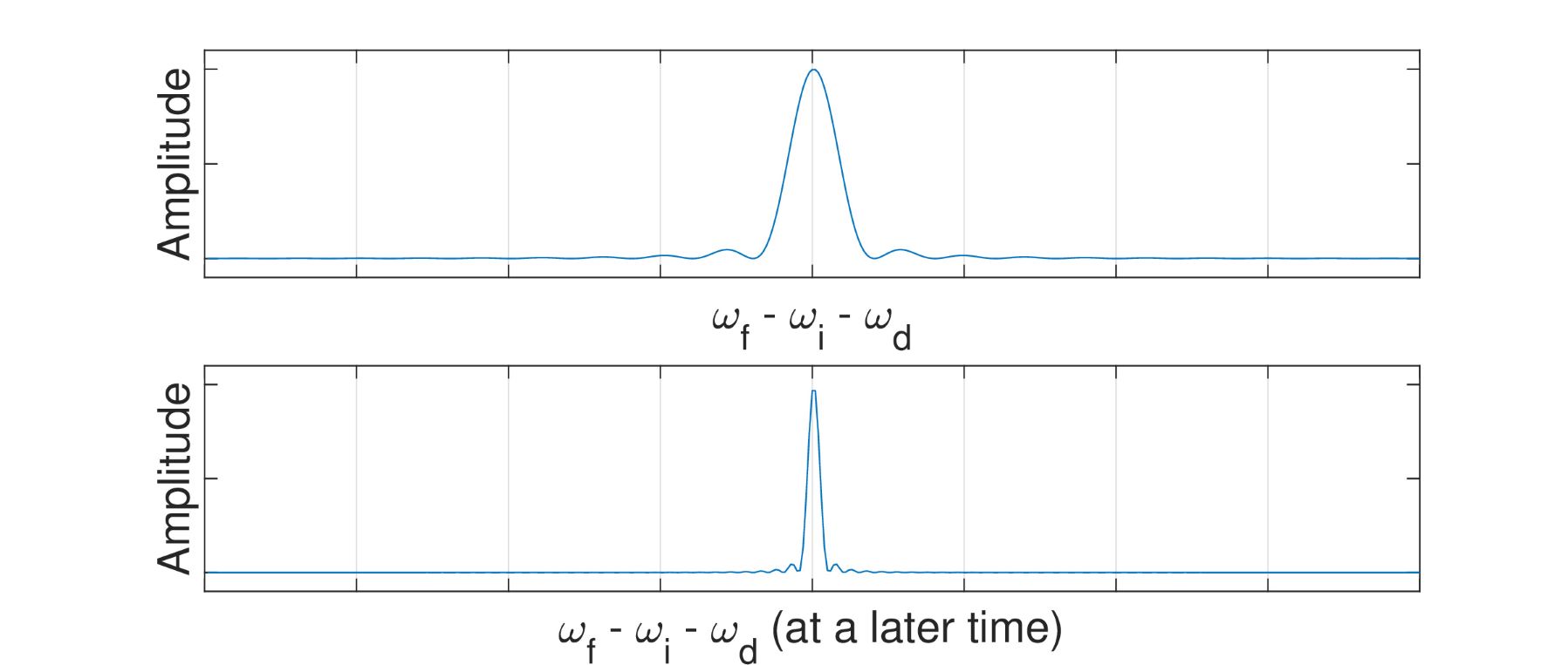
Figure 10: Fermi’s Golden Rule, transition amplitude. There is more than one possible interpretation for this plot. (Top) For a given driving frequency, we treat the energy jump $\omega_{fi}$ as the variable. The greatest amplitude occurs when $\omega_{fi}$ matches the driving frequency, $\omega_{d}$. (Bottom) At a later time the resonance curve has changed, so this can serve to predict time evolution despite that it is a distribution in $\omega$ space.

Consider Fermi’s Golden Rule: a bound state $\omega_{i}$ transitions to a continuum state $\omega_{f}$ under a driving frequency $\omega_{d}$, producing the transition amplitude expressed in Eq. 11. By varying $\omega_{d}$, $\omega_{i}$, or $\omega_{f}$, fig. 10 is useful for identifying the relevant dependencies.

However, fig. 10 can also be interpreted time-wise because the $sinc$ function depends symmetrically on time and energy. Over time, the $sinc$ function (as a function of $\omega_{fi}-\omega_{d}$) becomes more peaked, and the image in fig. 10 is considered to be a snapshot of time. Thus, we interpret the amplitude as time-dependent, $c(t)$.

However, this interpretation misreads the proper domain. Amplitude $c_{fi}$ is a frequency distribution and not a time distribution. The time dependence is implicit; evolving time means updating the entire distribution, after which we can derive the frequency-dependent amplitude at that time.

These processes are distinct. The former involves only number reading from the graph, while the latter requires repeated graphing and sampling. The former is a function, whereas the latter is a functional.

The same reasoning applies to the usual kicked harmonic oscillator treatment (perturbed by a small Gaussian pulse, Section II.1). The standard methods lead to the coefficient in Eq. 14, which is implicitly defined by the elapsed time $T$ but explicitly a function of $\omega$. This can help determine the best pulse duration $T$ to match the natural oscillator frequency $\omega$, but it overshadows the more natural $c=c(\omega)$ dependence.

Each $\Delta t$ value is a unique experiment leading to a different distribution. In varying $\Delta t$, Eq. 14 becomes a functional by creating a configuration space for each $\Delta t$ value.

Supplemental materials

Appendix S1 Accuracy of method

To analyze the accuracy of Eqs. 9, 24 and 25, we used MATLAB to compare the convolution method and the method of direct integration of the Schrödinger equation in Eq. 16.

S1.1 Comparing first-order to second-order convolution

The first-order contributions and second-order corrections for the convolution (or recursive Fourier transform) method were compared, as shown in Fig. 5. The second-order contribution shortens the central peak, while heightening the wings of the distribution by a small amount. This is reasonable because we expect the potential to deflect the system away from its original state each time it is applied.

S1.2 Frequency profile versus potential strength

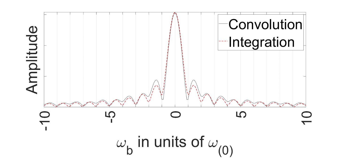
(a) Low potential.

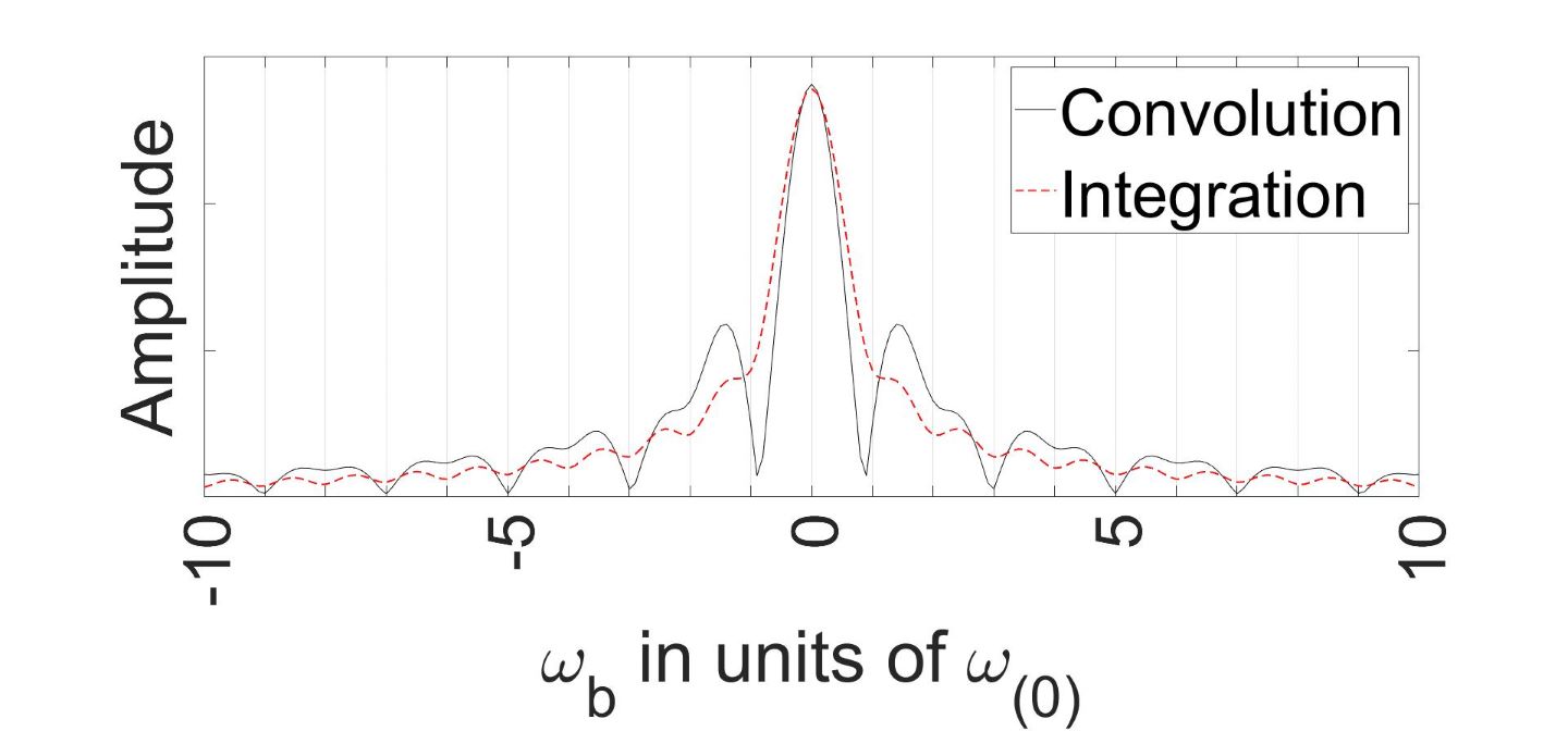
(b) Medium potential.

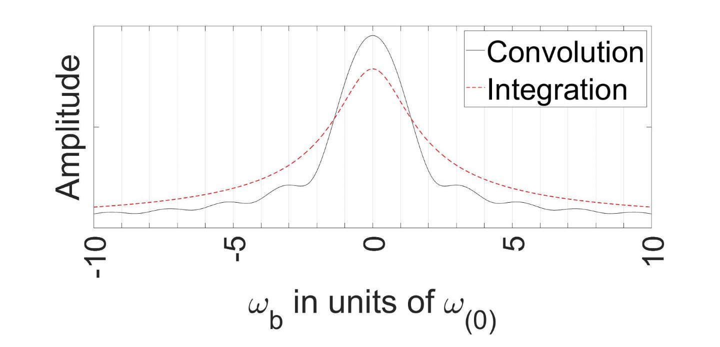
(c) High potential.

Figure S1: Second-order comparison of spectra for various values of the potential for convolution versus integration methods.

For the measurement of duration $T$, figs. 1(a)-1(c) show the second-order amplitude calculated by direct integration and convolution. In both methods, increasing the potential spreads the central peak and smoothens the ripples in the distribution. For a given increase in the potential strength, the ripples are preserved to a greater extent in the convolution method. Furthermore, the smoothing occurred differently in both cases. In particular, fig. 1(b) shows that for the convolution method, the odd-numbered zero-crossings are preserved longer than the even ones, as the potential strength is increased.

S1.3 Frequency profile versus range of intermediate states

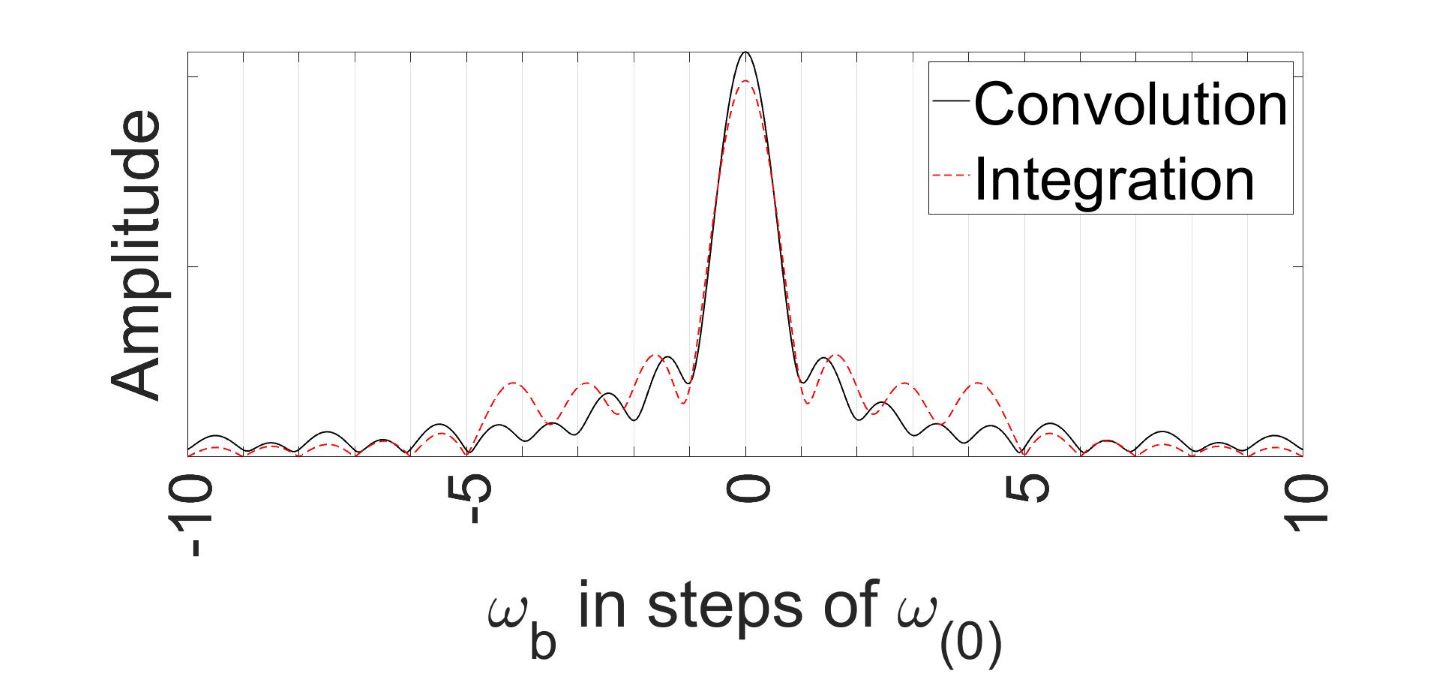
(a) $b_{max}=\pm 4$

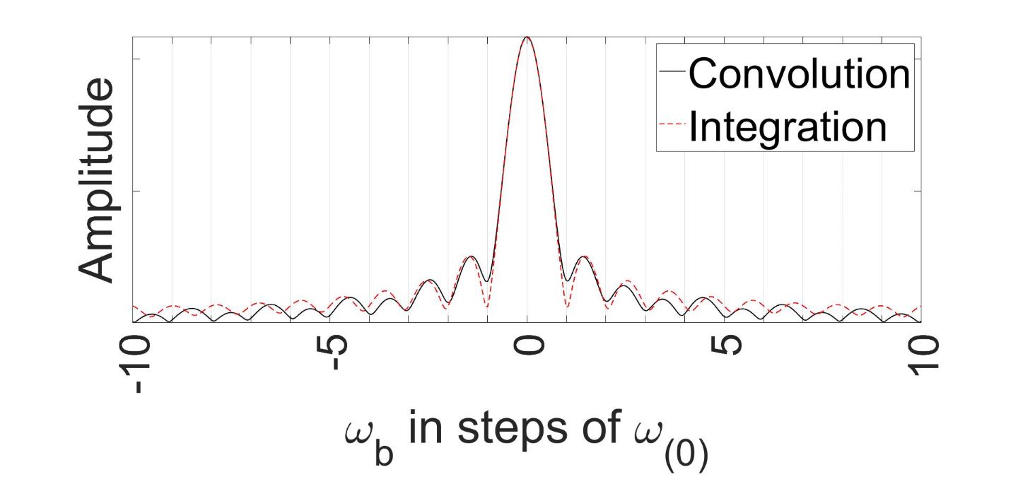
(b) $b_{max}=\pm 10$

Figure S2: Second-order comparison of spectra for two values of the $b_{max}$ range for convolution versus integration methods. The methods match each other more closely far from the origin as more $b$ terms are added.

Figs. 2(a)-2(b) demonstrate the distinct behavior of direct integration versus convolution with respect to the number of intermediate states $b_{max}$ that are summed over. The convolution method converges faster than the direct integration with respect to the number of intermediate terms included. The convolution method relies heavily on non-local surrounding states. This is not surprising when considering the similarity between Eqs. 24-25 to the $sinc$ interpolation signal reconstruction (as shown in Section S2.2).

Appendix S2 Interpretation

S2.1 Kicked frequency and natural frequency for harmonic oscillator

Eq. 25 presents two distinct energy scales: the unperturbed harmonic oscillator’s discrete spacing $\omega_{(0)}$, and the truncated perturbation-induced minima spacing $\omega_{(1)}=2\pi/T$. The latter corresponds to the $sinc$ function zeros in Eq. 9 and 25. This truncated perturbation is comparable to the periodic kick potential in the Floquet theory, where the Hamiltonian splits into a free part (with a discrete eigenspectrum) and a kick part (with a continuous eigenspectrum).

The unitary evolution operator $\hat{U}$ comprises $\hat{U}_{free}$, which determines $\omega_{(0)}$ and the unperturbed basis states, and $\hat{U}_{kick}$, which establishes $\omega_{(1)}$.

The dynamics of a Floquet system strongly hinge on the relationship between the natural frequencies of the two Hamiltonian parts: $\omega_{(1)}$ and $\omega_{(0)}$. Engels [36] investigated structured stochastic webs arising in the phase space for various energy scale values. When these two are integer ratios, the phase-space web is distinct, with clear allowed and forbidden regions. By contrast, when the two are irrational, the web structure collapses, allowing the entire phase space. Floquet systems show that the discrete energy states $\omega_{(0)}$ endure through time evolution, whereas the continuous states defined by $\omega_{(1)}$ disperse.

This scenario underscores the distinction between oscillator frequency $\omega_{(0)}$, and perturbation frequency $\omega_{(1)}$ [36]. We focused on the ”cyclotron resonance” case in fig. 8 and the subsequent graphs, where $\omega_{(0)}=\omega_{(1)}$. Here, the periodic kicks of the Floquet system coincided with the natural motion of the unperturbed oscillator.

S2.2 Frequency sampling interpretation

It is interesting to note the similarity between Eq. 9 and the Shannon-Nyquist sampling theorem

$$\begin{split}f(t)=\sum_{i}f(n\Delta t)\cdot sinc(\omega t-n\pi).\end{split}$$ (47)

The theorem states that any signal $f(t)$ can be exactly reconstructed from its samples, $f(n\Delta t)$, using a series of ideal $sinc$ interpolation functions centered on each sample, separated by a Nyquist period.

In the case of Eq. 9, a signal in the frequency domain, $c(\omega)$ is smoothly reconstructed from discrete samples, $c(n\Delta\omega_{(0)})$, using a series of $sinc$-like interpolation functions centered on each energy eigenstate. In the case of zero potential ($\tilde{V}(\omega)=\delta(\omega)$), if we constrain the measurement window to be the inverse of the oscillator frequency, $T=1/\omega_{(1)}=1/\omega_{(0)}$, then Eq. 9 exactly reconstructs the original wavefunction with an ideal $sinc$ interpolator. As the perturbation increases from zero, the interpolation function changes, and the reconstructed signal is no longer identical to the original.

References

- Schrödinger [926e] E. Schrödinger, Quantisierung als eigenwertproblem (vierte mitteilung), Ann. Phys. 81 (1926e).
- Dirac [1930] P. A. M. Dirac, The Principles of Quantum Mechanics (Oxford: Clarendon Press, 1930).
- Dyson [1952] F. J. Dyson, Divergence of perturbation theory in quantum electrodynamics, Phys. Rev. 85, 631 (1952).
- Schwartz [2014] M. D. Schwartz, Quantum Field Theory and the Standard Model (Cambridge University Press, 2014).
- Walker and Gathright [1994] J. S. Walker and J. Gathright, Exploring one-dimensional quantum mechanics with transfer matrices, Am. J. Phys. 62 (1994).
- Feynman [1948] R. P. Feynman, Space-time approach to non-relativistic quantum mechanics, Rev. Mod. Phys. 20, 367 (1948).
- Feynman [948ba] R. P. Feynman, A relativistic cut-off for classical electrodynamics, Phys. Rev. 74, 939 (1948ba).
- Feynman [948bb] R. P. Feynman, A relativistic cut-off for classical electrodynamics, Phys. Rev. 74, 1430 (1948bb).
- Schroeter [2018] D. J. G. D. F. Schroeter, Introduction to Quantum Mechanics, 3rd Edition (University Cambridge Press, 2018).
- Paganin and Pelliccia [2021] D. M. Paganin and D. Pelliccia, X-ray phase-contrast imaging: a broad overview of some fundamentals, Adv. Imaging Electron Phys. 218, 63 (2021).
- Strang [1968] G. Strang, On the construction and comparison of difference schemes, SIAM Journal on Numerical Analysis 5, 506 (1968).
- Kosloff and Kosloff [1983] D. Kosloff and R. Kosloff, A fourier method solution for the time dependent schrödinger equation as a tool in molecular dynamics, Journal of Computational Physics 52, 35 (1983).
- Dateo et al. [1991] C. E. Dateo, V. Engel, R. Almeida, and M. Horia, Numerical solutions of the time-dependent schrödinger equation in spherical coordinates by fourier transform methods, Computer Physics Communications 63, 435 (1991).
- Van Dyck [1985] D. Van Dyck, Image calculations in high-resolution electron microscopy: Problems. progress. and prospects, Adv. Electron. Electron. Phys. 65, 295 (1985).
- Taha and Ablowitz [1984] T. R. Taha and M. I. Ablowitz, Analytical and Numerical Aspects of Certain Nonlinear Evolution Equations. II. Numerical, Nonlinear Schrödinger Equation, Journal of Computational Physics 55, 203 (1984).
- Bandrauk and Shen [1992] A. D. Bandrauk and H. Shen, Higher order exponential split operator method for solving time-dependent schrodinger equations, Can. J. Chem 70 (1992).
- Hansson and Wabnitz [2016] T. Hansson and S. Wabnitz, Dynamics of microresonator frequency comb generation: Models and stability, Nanophotonics 5 (2016).
- Nelson-Isaacs [2021] S. E. Nelson-Isaacs, Spacetime paths as a whole, Quantum reports 3, 13 (2021).
- Tamma and Laibacher [2015] V. Tamma and S. Laibacher, Multiboson correlation interferometry with arbitrary single-photon pure states, Physical Review Letters 114, 243601 (2015).
- Laibacher and Tamma [2018] S. Laibacher and V. Tamma, Symmetries and entanglement features of inner-mode-resolved correlations of interfering nonidentical photons, Phys. Rev. A 98, 053829 (2018).
- Tamma and Laibacher [2021] V. Tamma and S. Laibacher, Boson sampling with random numbers of photons, Phys. Rev. A 104, 032204 (2021).
- Tamma and Laibacher [2023] V. Tamma and S. Laibacher, Scattershot multiboson correlation sampling with random photonic inner-mode multiplexing, The European Physical Journal Plus 138, 335 (2023).
- Wang et al. [2018] X.-J. Wang, B. Jing, P.-F. Sun, C.-W. Yang, Y. Yu, V. Tamma, X.-H. Bao, and J.-W. Pan, Experimental time-resolved interference with multiple photons of different colors, Phys. Rev. Lett. 121, 080501 (2018).
- Triggiani et al. [2023] D. Triggiani, G. Psaroudis, and V. Tamma, Ultimate quantum sensitivity in the estimation of the delay between two interfering photons through frequency-resolving sampling, Physical Review Applied 19, 044068 (2023).
- Gottlieb and Wesoloski [2006] A. D. Gottlieb and L. Wesoloski, Bardeen’s tunneling theory as applied to scanning tunneling microscopy: A technical guide to the traditional interpretation, Nanotechnology 17, 10.1088/0957-4484/17/8/R01 (2006).
- J. M. Zhang [2016] Y. L. J. M. Zhang, Fermi’s golden rule: its derivation and breakdown by an ideal model, Eur. J. Phys. 37, https://doi.org/10.1088/0143-0807/37/6/065406 (2016).
- Note [1] Switching the order of the sum and the integral in an infinite series can have unpredictable effects on the convergence of the series in general, but for our purposes we only examine the second-order expansion. This poses the same limitation on validity as other variational approaches such as Feynman diagrams.
- Tamma and Laibacher [2016] V. Tamma and S. Laibacher, Boson sampling with non-identical single photons, Journal of Modern Optics 63, 41 (2016).
- Li et al. [2008] X. Li, X. Ma, Z. Y. Ou, L. Yang, L. Cui, and D. Yu, Spectral study of photon pairs generated in dispersion shifted fiber with a pulsed pump, Opt. Express 16, 32 (2008).
- Chen et al. [2005] J. Chen, X. Li, and P. Kumar, Two-photon-state generation via four-wave mixing in optical fibers, Phys. Rev. A 72, 033801 (2005).
- Sharping et al. [2004] J. E. Sharping, J. Chen, X. Li, P. Kumar, and R. S. Windeler, Quantum-correlated twin photons from microstructure fiber, Opt. Express 12, 3086 (2004).
- Garay-Palmett et al. [2007] K. Garay-Palmett, H. J. McGuinness, O. Cohen, J. S. Lundeen, R. Rangel-Rojo, A. B. U’Ren, M. G. Raymer, C. J. McKinstrie, S. Radic, and I. A. Walmsley, Photon pair-state preparation with tailored spectral properties by spontaneous four-wave mixing in photonic-crystal fiber, Opt. Express 15, 14870 (2007).
- Keller and Rubin [1997] T. E. Keller and M. H. Rubin, Theory of two-photon entanglement for spontaneous parametric down-conversion driven by a narrow pump pulse, Phys. Rev. A 56, 1534 (1997).
- Rubin et al. [1994] M. H. Rubin, D. N. Klyshko, Y. H. Shih, and A. V. Sergienko, Theory of two-photon entanglement in type-ii optical parametric down-conversion, Phys. Rev. A 50, 5122 (1994).
- Note [2] The non-linearity is contained in the expression with , but is not important for this derivation.
- Engel [2007] U. M. Engel, On Quantum Chaos, Stochastic Webs and Localization in a Quantum Mechanical Kick System (Logos Verlag, 2007).