Significance Bands for Local Projections 

Abstract

An impulse response function describes the dynamic evolution of an outcome variable following a stimulus or treatment. A common hypothesis of interest is whether the treatment affects the outcome. We show that this hypothesis is best assessed using significance bands rather than relying on commonly displayed confidence bands. Under the null hypothesis, we show that significance bands are trivial to construct with standard statistical software using the LM principle, and should be reported as a matter of routine when displaying impulse responses graphically.

JEL classification codes: C11, C12, C22, C32, C44, E17.

Keywords: local projections, impulse response, instrumental variables, significance bands, wild block bootstrap.

1.   Introduction

Practitioners routinely display impulse response estimates surrounded by confidence bands to graphically illustrate the uncertainty of the estimated response coefficients given the sample. These bands are often calculated using point-wise inference, such as when one inverts the standard Wald $t$-statistic. However, it is well-known that such bands—whether constructed using classical, bayesian, bootstrap or other simulation methods—cannot be directly used to assess joint hypotheses of whether the coefficients are zero or not (see, e.g. Jordà, , 2009; Inoue & Kilian, , 2013, 2016; Montiel Olea & Plagborg-Møller, , 2019). Nevertheless, they are commonly used as a back-of-the-envelope check of the statistical significance of the impulse response—the null hypothesis that an intervention or treatment generates no response in the outcome.

This is problematic. Impulse response coefficients are highly correlated. In a small sample, these coefficients may be individually imprecisely estimated while at the same time following a joint trajectory that is clearly different from zero in the statistical sense. The problem is similar to that in near collinear regression—where individual $t$-statistics are no different from 0, but an $F$-test clearly is. A typical example is presented in Figure 1. The figure shows the response of 100 $\times$ the log of the consumer price index (CPI) in the U.S in response to a Romer monetary shock (Romer & Romer, , 2004). Note that the (1 and 2 standard error) confidence bands displayed include 0 at all horizons and thus, one is tempted to conclude that a monetary shock has no impact on inflation. However, the test of the joint null that all response coefficients are zero is easily rejected, with a p-value of 1.97e-17. We shall argue that there is a more formal and simpler way to graphically display the natural null hypothesis of whether an impulse response differs from zero by using significance bands and local projections (Jordà, , 2005), or non-linear impulse responses as in Angrist et al., (2016). For brevity we only consider the linear case in this paper.

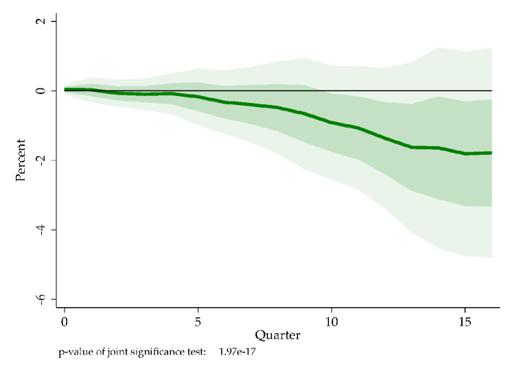
Figure 1: Cumulative response of the CPI in percent to a Romer monetary shock

Notes: impulse response of 100 $\times$ log CPI to a Romer monetary shock (Romer & Romer, , 2004) as extended by Wieland & Yang, (2020). The specification includes four lags of CPI inflation, GDP growth, and a one year T-Bill rate. The sample is 1969:Q1 - 2007:Q4. Dark/light shaded region is for one/two-standard error bands. See text.

Under the null hypothesis and using the Lagrange multiplier (LM) principle, inference is greatly simplified. In general settings, we show that inference is independent of the impulse response horizon. Moreover, we provide analytic formulas that are trivial to implement with standard statistical software. In addition, we discuss bootstrap methods that make fewer assumptions on the data generating process. Monte Carlo evidence shows that these methods provide the desired level of probability coverage.

The intuition for our procedures is similar to that for the significance bands common in correlogram plots. In time series analysis, the asymptotic $\pm 1.96/\sqrt{n}$ bands displayed in correlograms are a special case of our significance bands. Under the null hypothesis of no serial correlation, the data are a white noise process. In small samples, its autocorrelations will not be exactly zero, but will attain values inside the significance bands if the null is true. A correlogram is, in fact, an impulse response for an AR(1) model. Whenever an autocorrelation surpasses the $\pm 1.96/\sqrt{n}$ barrier, that coefficient can be deemed to be different from zero, and one or more rejections would be enough to reject the white noise null.

Should a practitioner then display confidence or significance bands? We argue for both. Each serves a different purpose. Thought of as the interval where the most probable values of the response are to be found, it is natural to plot confidence bands at one standard deviation values, as is common practice, since this represents a natural compromise between probability coverage and interval width. In contrast, significance bands should be displayed at conventional probability levels, that is at a 90% or 95% coverage. The reason is that the significance band is being used to evaluate a scientific hypothesis that is central to almost every empirical analysis: does an intervention/treatment generate a statistically significant response/effect? The significance band is a visualization of this hypothesis test.

2.   The basic set up and intuition

Suppose one is interested in estimating the following impulse response function:

$$\mathcal{R}_{y}(h)\equiv E(y_{t+h}|s_{t}=s_{0}+\delta;\bm{x}_{t})-E(y_{t+h}|s_{t}=s_{0},\bm{x}_{t})\quad\text{for }h=0,1,\ldots,H-1$$ (1)

where $s$ is the impulse, intervention, or treatment variable, $\delta$ is the dose (how big the intervention is), $s_{0}$ is the initial value from which the effect of the treatment is being evaluated (in a linear model this will not matter, of course), and $\bm{x}_{t}$ is a vector of exogenous and pre-determined variables, including the constant, time trends, and lags of the outcome and intervention variables. The variable $y$ is the outcome variable of interest.

Assume the researcher approximates Equation 1 using linear local projections, the most common application seen in the literature. Further, to make the notation more transparent and to take advantage of our linearity assumption, we can appeal to the Frisch-Waugh-Lovell theorem so that one can think of $y_{t+h}$ and $s_{t}$ as having been previously orthogonalized with respect to the rich set of controls in $\bm{x}_{t}$. Hence $y_{t}$ and $s_{t}$ also have a zero mean. Moreover and for later use, we also assume that an instrument $z_{t}$ for $s_{t}$ is available and has been previously orthogonalized with respect to $\bm{x}_{t}$ as well. Thus, from this point forward, the notation can be interpreted to refer to these orthogonalized variables and we will not indicate so explicitly to keep the notational burden at a minimum.

Given this preliminary discussion, the local projections estimator of Equation 1 can be obtained from the instrumental variables regression:

$$y_{t+h}=s_{t}\beta_{h}+u_{t+h}\quad\text{for }h=0,1,\ldots,H-1;\quad t=1,\ldots,T$$ (2)

We assume that $z_{t}$, meets the usual conditions for relevance, lead-lag exogeneity (see, e.g. Stock & Watson, , 2018), and the exclusion restriction. That is:

• Relevance: $E(s_{t}\,z_{t})\neq 0$.

• Lead-lag exogeneity: $E(u_{t+h}\,z_{t})=0\,\forall h$.

• Exclusion restriction: $E(y_{t+h}\,z_{t}|s_{t})=0$.

Note that depending on the setting, $z_{t}$ may include $s_{t}$ itself, such as when $s_{t}$ is an observable shock, and then the discussion returns to a more traditional OLS setting. Or if $s_{t}$ is conditional $x_{t}$, sequentially exogenous. This would be the case in a recursive identification scheme. We further assume that $y_{t}$, $s_{t}$, and $z_{t}$ are covariance stationary. This assumption is not necessary to ensure consistency of the local projection, but will make deriving our inferential procedures and the presentation in this section straightforward.

Based on this simple set up, the instrumental variable estimator for $\beta_{h}$ can be written as:

$$\sqrt{T-h}(\hat{\beta}_{h}-\beta_{h})=\frac{(T-h)^{-1/2}\sum_{1}^{n}z_{t}\>y_{t+h}}{(T-h)^{-1}\sum_{1}^{n}z_{t}\>s_{t}}\quad\text{for }h=0,1,\ldots,H-1,$$ (3)

where we note that we will evaluate the statistic under the null $H_{0}:\beta_{h}=0$. Under standard regularity conditions (made more precise below) and the instrumental variable assumptions for local projections, it is easy to see that:

$$\frac{1}{T-h}\sum_{1}^{n}z_{t}\>s_{t}\overset{p}{\to}E(z_{t}\>s_{t})\equiv\gamma_{zs}$$ (4)

Next, consider the numerator in Equation 3 evaluated at the null $H_{0}:\beta_{h}=0$:

$$\frac{1}{(T-h)^{1/2}}\sum_{1}^{n}z_{t}\>y_{t+h}\overset{d}{\to}N(0,\omega)$$ (5)

where $\omega$ is given by:

$$\omega=Var\left(\frac{1}{(T-h)^{1/2}}\sum_{1}^{n}z_{t}\>y_{t+h}\right) \>\approx\sum_{j=-\infty}^{\infty}E(z_{t}\>y_{t+h}\>z_{t-j}\>y_{t+h-j})$$

$$\>=\sum_{j=-\infty}^{\infty}E(z_{t}\>z_{t-j})E(y_{t+h}\>y_{t+h-j})$$

$$\>=\sum_{j=-\infty}^{\infty}\gamma_{z,j}\>\gamma_{y,j}$$ (6)

where the second equality follows from the lead-lag exogeneity assumption and the null hypothesis that $\beta_{h}=0$ for $h=0,1,\ldots,H-1$. We define $\gamma_{z,j}$ and $\gamma_{y,j}$ as the $j^{th}$ autocovariances of $z$ and $y$ respectively. Importantly, note that $\omega$ is not a function of the horizon $h$.

Putting things back together, we can write Equation 3 under the null hypothesis as:

$$\sqrt{T-h}(\hat{\beta}_{h}-0)\overset{d}{\to}N(0,\sigma^{2});\quad\sigma^{2}=\frac{\sum_{j=-\infty}^{\infty}\gamma_{z,j}\gamma_{y,j}}{\gamma_{zs}^{2}}=\frac{\omega}{\gamma_{zs}^{2}};\quad\forall h$$ (7)

From Equation 7 it is easy to derive a $1-\alpha$ percent band around the zero null so that:

$$P\left[\zeta_{\alpha/2}\,\frac{\sigma}{\sqrt{T-h}}<\hat{\beta}_{h}<\zeta_{(1-\alpha/2)}\,\frac{\sigma}{\sqrt{T-h}}\right]=1-\alpha$$

where $\zeta_{\alpha/2}$ is the critical value of a standard normal variable at $\alpha/2$ and for a standard normal, $\zeta_{1-\alpha/2}=-\zeta_{\alpha/2}$, as is well known. to construct feasible confidence intervals we need to replace $\sigma$ with an estimate. The LM principle requires that $\sigma$ be estimated using the conventional formula for HAC robust standard errors for the just identified two-stage least squares estimator, but evaluated at $\beta_{h}=0$. This is accomplished by estimating $\omega$ with the long-run variance of $\eta_{t}=z_{t}y_{t+h}$, which is equal to $s_{\eta}^{2}=\sum_{j=-\infty}^{\infty}E(\eta_{t}\eta_{t+j})$.

When plotting a significance band of an impulse response up to $H-1$ periods, we are essentially conducting a joint hypothesis test. Intuitively, the more horizons considered, the more likely it is to spuriously reject the null when the null is true in a finite sample. A simple way to address this issue is with a Bonferroni adjustment as proposed in Dunn, (1961) so that the significance bands for each $\hat{\beta}_{h}$ become:

$$\left[\zeta_{\alpha/2H}\frac{\sigma}{\sqrt{T-h}},\,\,\zeta_{1-\alpha/2H}\frac{\sigma}{\sqrt{T-h}}\right].$$

The joint probability that the estimated impulse response lies within the confidence band is given by:

$$P\left(\bigcap_{h=0}^{H-1}\left\{\zeta_{\alpha/2H}\,\frac{\sigma}{\sqrt{T-h}}<\hat{\beta}_{h}<\zeta_{(1-\alpha/2H)}\,\frac{\sigma}{\sqrt{T-h}}\right\}\right)\geq 1-\alpha$$ (8)

where the inequality holds in large samples and when the null hypothesis of a zero response is true. Similarly, the test of the joint hypothesis that all response coefficients are zero rejects when:

$$\hat{\beta}_{h}\not\in\left[\zeta_{\alpha/2H}\frac{\sigma}{\sqrt{T-h}},\,\,\zeta_{1-\alpha/2H}\frac{\sigma}{\sqrt{T-h}}\right]$$

for at least one $h$. By the same argument, it follows that the size of such a test is not more than $\alpha$ in large samples.

A simple example provides further intuition and a connection to well-known results. In the special case where $z=s$, and $y$ and $s$ are serially uncorrelated, this expression simplifies even further to:

$$\sigma^{2}=\frac{\gamma_{y,0}}{\gamma_{s,0}}$$

Thus, when $y=s=z$ and $y$ is a white noise and hence $\gamma_{y,0}=\gamma_{s,0}$ so that $\sigma^{2}=1$, the local projection estimator is simply an estimator of the autocorrelation function. Hence, applying the same derivations as in Equation 7, it is easy to see that one recovers the well known bands for the autocorrelogram of $y$. Specifically, focus on $h=1$ in the special case that $y$ is a white noise but one estimates an AR(1) model:

$$\sqrt{n}(\hat{\rho}-0)\overset{d}{\to}N(0,1).$$ (9)

This is the well known case where the 95% asymptotic significance bands in a correlogram are calculated as $\pm 1.96\times 1/\sqrt{n}$ and provides a nice window into our proposed procedures. Importantly, notice that the bands do not depend on the horizon (in fact, they also do not depend on the variance in this special case). Whenever an autocorrelation coefficient exceeds the band, the interpretation is that said coefficient can be deemed to be different from zero. This, of course, means that the hypothesis that the impulse/treatment has no effect on the outcome can be rejected.

2.1.   Practical implementation

Constructing significance bands in practice based on the results from the previous section is straightforward and can be implemented using standard statistical software. The online appendix contains a STATA example to illustrate this point and corresponds to the figures displayed in the paper. The basic steps can be summarized as follows:

 Significance bands using asymptotic approximations  

1. Calculate the sample average of the product $s_{t}\,z_{t}$. Call this $\hat{\gamma}_{sz}$.

2. Construct the auxiliary variable $\eta_{t}=y_{t}\,z_{t}$ and regress $\eta_{t}$ on a constant. The Newey-West estimate of the standard error of the intercept coefficient is an estimate of $s_{\hat{\eta}}$.

3. An estimate of $\sigma/\sqrt{T-h}\,$, call it $\hat{s}_{\beta_{h}}\,$, is therefore:

   $$\hat{s}_{{\beta}_{h}}=\frac{\hat{s}_{{\hat{\eta}}}}{\hat{\gamma}_{sz}}$$

4. Construct the significance bands as:

   $$\left[\zeta_{\alpha/2H}\hat{s}_{{\beta}_{h}},\,\,\zeta_{1-\alpha/2H}\hat{s}_{\beta_{h}}\right]$$

 

A bootstrap procedure is equally easy to construct. Note that we do not take a position on the data generating process (DGP). Therefore, we apply the bootstrap directly to step 2 of the previous construction of the significance band. Because of the time series dependence and the possible existence of heteroscedasticity, we will use a wild-block bootstrap (see, e.g. Gonçalves & Kilian, , 2007). The online appendix provides the STATA implementation, which only requires a few lines of code. Thus, the entire procedure can be described as follows:

 Significance bands using the Wild-Block Bootstrap  

1. Calculate the sample average of $s_{t}\,z_{t}$. Call this $\hat{\gamma}_{sz}$.

2. Construct the auxiliary variable $\eta_{t}=y_{t}\,z_{t}$ and regress $\eta_{t}$ on a constant. The Wild Block bootstrap estimate of the standard error of the intercept coefficient is an estimate of $s_{\hat{\eta}}$.

3. An estimate of $\sigma/\sqrt{T-h}\,$, call it $\hat{s}^{b}_{\beta_{h}}\,$, is therefore:

   $$\hat{s}^{b}_{{\beta}_{h}}=\frac{\hat{s}^{b}_{{\hat{\eta}}}}{\hat{\gamma}_{sz}}$$

4. Construct the significance bands as:

   $$\left[\zeta_{\alpha/2H}\hat{s}^{b}_{{\beta}_{h}},\,\,\zeta_{1-\alpha/2H}\hat{s}^{b}_{\beta_{h}}\right]$$

 

Using these procedures, we can now revisit Figure 1. Figure 2 presents the original impulse response figure but with significance bands constructed using the asymptotic approximation (in blue) and using the bootstrap (in red). As the figure shows, the result from using either procedure are virtually identical. Based on the significance bands displayed in the figure, we would conclude that there is essentially no response of inflation to monetary policy for the first year and a half, but thereafter, there is ample evidence that the response is non-zero, consistent with the significance joint hypothesis test p-value of 1.97e-17. The fact that the significance band is tighter than the confidence band is specific to this example and not a general feature of the relationship between significance and confidence bands.

Figure 2: Cumulative response of the CPI in percent to a Romer monetary shock

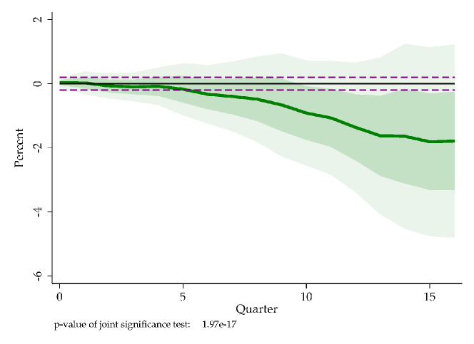
(a) Significance bands displayed

Notes: impulse response of 100 $\times$ log CPI to a Romer monetary shock (Romer & Romer, , 2004) as extended by Wieland & Yang, (2020). The specification includes four lags of CPI inflation, GDP growth, and a one year T-Bill rate. The sample is 1969:Q1 - 2007:Q4. 95% significance bands displayed, classical in blue and bootstrap in red. The dark/light shaded areas correspond to one/two standard error bands. See text.

3.   Monte Carlo evidence

This section presents a couple of simple experiments in graphical form to assess the calculation of significance bands using both the asymptotic approximation and the wild block bootstrap procedures discussed in the previous section. The data are generated as follows:

$$\begin{cases}y_{t}=\beta s_{t}+0.75y_{t-1}+u_{yt}\\ s_{t}=0.5s_{t-1}-0.25y_{t-1}+z_{t}+u_{st}\\ z_{t}=u_{zt}\end{cases}\quad u_{yt},\,u_{st},\,u_{zt}\,\sim\,N(0,1);\quad\beta\in\{0,0.25,0.50,0.75\}$$

This simple system encapsulates several features. First, the treatment variable, $s_{t}$, affects the outcome, $y_{t}$, contemporaneously. The outcome is itself serially correlated with a coefficient $0.75$. The idea is to have internal propagation dynamics. Next, the intervention responds to feedback from the value of the outcome in the previous period, but also has some internal propagation dynamics. In addition, movements in the intervention are caused by the exogenous variable $z_{t}$, which will act as our instrumental variable. Finally, the coefficient $\beta$, which captures the effect of the treatment on the outcome, has values between 0 and 0.75. When $\beta=0$ we have the null model with which to assess the size of the test. Increasing the value of $\beta$ allows us to assess the power of the significance bands.

We generate samples of 100, and 500 observations with 500 burn-in observations that are discarded to avoid initialization problems. For each sample size and for the different values of $\beta$ we generate 1,000 Monte Carlo replications. The implementation of the Wild Block bootstrap is based on 1,000 bootstrap replications as well. For the Newey-West step as well as for the block size in the bootstrap, we use 8 lags. Figure 3 displays the results for sample sizes of 100 and 500 observations.

The figure summarizes quite a bit of information. The shaded bands around the mean estimate of the impulse response showcase the $25^{th}$ and the $975^{th}$ largest values for each coefficient estimate in the Monte Carlo simulation. The dashed lines correspond to the significance bands. Both Newey-West and the bootstrap procedures (using 8 lags) generate nearly indistinguishable values so the differences cannot be seen with the naked eye. For each Monte Carlo exercise, we construct rejection rates for each type of band constructed. The rate is calculated as the share of replications where one or more impulse response coefficients exceed the significance bands.

Several results deserve comment. First, consider the size of the test. We have chosen a rather conservative strategy with a window of size 8 both for Newey-West and for the block-size in the implementation of the bootstrap. As a result, with a small sample of 100 observations, the size is about 10% instead of the nominal 5%, though with 500 observations the size is close to 4%. However, even with this conservative choice, the power of the test is respectable with a sample size of 100, improving from about 25% when $\beta=0.25$ to about 95% when $\beta=0.75$. These numbers jump with 500 observations with about 95% for $\beta=0.25$ and 100% even for $\beta=0.5$.

Figure 3: Significance Bands: Monte Carlo exercise

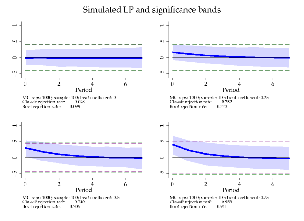
(a) Sample size: 100

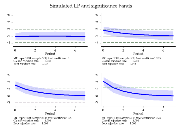
(b) Sample size: 500

Notes: Monte Carlo exercise. Sample size = 100 and 500 observations (500 burn-in replications). Significance bands constructed using asymptotic approximations (Classic) and the Wild Block bootstrap (Boot). The rejection rate refers to the share of replications where one or more coefficients exceed the significance bands constructed with each procedure. Treat coefficient refers to the coefficient $\beta$ described in the text. Significance bands constructed at 95% confidence level. Thus, when Treat coefficient = 0, the rejection rate should be 0.05, otherwise, it should be 1. See text.

4.   Conclusion

Significance bands should be displayed alongside confidence bands for local projections as a matter of routine. While confidence bands inform the reader about the estimation uncertainty of each coefficient, significance bands inform the reader about the significance of the impulse response itself. Formal tests of significance can and should be calculated, but these tests require estimation of local projections as a system. There are many settings where this is impractical. However, significance bands can be constructed with univariate regression using standard statistical software.

References

- Angrist et al., (2016) Angrist, Joshua D., Jordà, Òscar, & Kuersteiner, Guido M. 2016. Semiparametric Estimates of Monetary Policy Effects: String Theory Revisited. Journal of Business and Economic Statistics, http://dx.doi.org/10.1080/07350015.2016.1204919.
- Dunn, (1961) Dunn, Olive Jean. 1961. Multiple comparisons among means. Journal of the American statistical association, 56(293), 52–64.
- Gonçalves & Kilian, (2007) Gonçalves, Sílvia, & Kilian, Lutz. 2007. Asymptotic and bootstrap inference for AR () processes with conditional heteroskedasticity. Econometric Reviews, 26(6), 609–641.
- Inoue & Kilian, (2013) Inoue, Atsushi, & Kilian, Lutz. 2013. Inference on impulse response functions in structural VAR models. Journal of Econometrics, 177(1), 1–13.
- Inoue & Kilian, (2016) Inoue, Atsushi, & Kilian, Lutz. 2016. Joint confidence sets for structural impulse responses. Journal of Econometrics, 192(2), 421–432.
- Jordà, (2005) Jordà, Òscar. 2005. Estimation and Inference of Impulse Responses by Local Projections. American Economic Review, 95(1), 161–182.
- Jordà, (2009) Jordà, Òscar. 2009. Simultaneous Confidence Regions for Impulse Responses. The Review of Economics and Statistics, 91(3), 629–647.
- Montiel Olea & Plagborg-Møller, (2019) Montiel Olea, José Luis, & Plagborg-Møller, Mikkel. 2019. Simultaneous confidence bands: Theory, implementation, and an application to SVARs. Journal of Applied Econometrics, 34(1), 1–17.
- Romer & Romer, (2004) Romer, Christina D., & Romer, David H. 2004. A New Measure of Monetary Shocks: Derivation and Implications. American Economic Review, 94(4), 1055–1084.
- Stock & Watson, (2018) Stock, James H., & Watson, Mark W. 2018. Identification and Estimation of Dynamic Causal Effects in Macroeconomics Using External Instruments. The Economic Journal, 128(610), 917–948.
- Wieland & Yang, (2020) Wieland, Johannes F., & Yang, Mu-Jeung. 2020. Financial Dampening. Journal of Money, Credit and Banking, 52(1), 79–113.