A GALEX view of the DA White Dwarf Population

Abstract

We present a detailed model atmosphere analysis of 14001 DA white dwarfs from the Montreal White Dwarf Database with ultraviolet photometry from the GALEX mission. We use the 100 pc sample, where the extinction is negligible, to demonstrate that there are no major systematic differences between the best-fit parameters derived from optical only data and the optical + UV photometry. GALEX FUV and NUV data improve the statistical errors in the model fits, especially for the hotter white dwarfs with spectral energy distributions that peak in the UV. Fitting the UV to optical spectral energy distributions also reveals UV-excess or UV-deficit objects. We use two different methods to identify outliers in our model fits. Known outliers include objects with unusual atmospheric compositions, strongly magnetic white dwarfs, and binary white dwarfs, including double degenerates and white dwarf + main-sequence systems. We present a list of 89 newly identified outliers based on GALEX UV data; follow-up observations of these objects will be required to constrain their nature. Several current and upcoming large scale spectroscopic surveys are targeting $>10^{5}$ white dwarfs. In addition, the ULTRASAT mission is planning an all-sky survey in the NUV band. A combination of the UV data from GALEX and ULTRASAT and optical data on these large samples of spectroscopically confirmed DA white dwarfs will provide an excellent opportunity to identify unusual white dwarfs in the solar neighborhood.

1 Introduction

The Galaxy Evolution Explorer (GALEX) is the first space based mission to attempt an all-sky imaging survey in the ultraviolet (UV, Martin et al., 2005). In the ten years that it was operational, GALEX surveyed 26000 square degrees of the sky as part of the all-sky imaging survey in two band passes: Far Ultraviolet (FUV) and Near Ultraviolet (NUV) with central wavelengths of 1528 and 2271 Å  respectively (Morrissey et al., 2005). Although its primary goal was to study star formation and galaxy evolution, the depth ($m_{\rm AB}\approx 20.5$ mag) and the large sky coverage of the all-sky imaging survey provide an excellent opportunity to study UV bright objects like hot white dwarfs.

Prior to Gaia, the majority of the white dwarfs in the solar neighborhood were identified through Sloan Digital Sky Survey spectroscopy, which specifically targeted hot and blue white dwarfs as flux standards (e.g., Kleinman et al., 2013). Many of the SDSS white dwarfs have spectral energy distributions that peak in the UV. Hence, GALEX FUV and NUV data can help constrain the physical parameters of these white dwarfs. GALEX data will also be useful for cooler white dwarfs; UV photometry will be used to confirm the temperature derived from the optical data, or to constrain the far red wing of the Lyman $\alpha$ line that dominates the opacity in the blue part of the spectral energy distribution of cool hydrogen atmosphere white dwarfs (Kowalski & Saumon, 2006). Yet, GALEX data are under-utilized in the analysis of white dwarfs in the literature, perhaps due to the relatively strong extinction observed in the UV.

Wall et al. (2019) used 1837 DA white dwarfs with high signal to noise ratio spectra and Gaia parallaxes to verify the absolute calibration of the FUV and NUV data, and refined the linearity corrections derived by Camarota & Holberg (2014). They also empirically derived extinction coefficients for both bands, finding $R_{\rm FUV}=8.01$ and $R_{\rm NUV}=6.72$, where $R$ is the ratio of the total absorption $A_{\lambda}$ to reddening $E(B-V)$ along the line of sight to an object. Wall et al. (2019) highlighted the utility of their newly derived extinction coefficients for identifying white dwarfs with unusual UV photometry. By comparing the observed GALEX magnitudes to predictions from the model atmosphere calculations, they found 12 outliers in the UV, seven of which were previously known, including three double degenerates, two white dwarf + main-sequence star binaries, one ZZ Ceti, and one double degenerate candidate.

Lajoie & Bergeron (2007) compared the effective temperatures obtained from the optical and UV spectra of 140 DA white dwarfs from the IUE archive. They found that the optical and UV temperatures of the majority of stars cooler than 40000 K and within 75 pc are in fairly good agreement with $\Delta T_{\rm eff}/T_{\rm optical}\leq 10$%. They also found that the majority of the discrepancies between the two temperature measurements were caused by interstellar reddening, which affects the UV more than the optical. By restricting their analysis to white dwarfs within 75 pc, where the extinction is negligible, they were able to identify several double degenerate candidates, as well as a DA + M dwarf system, and stars with unusual atmospheric compositions. Lajoie & Bergeron (2007) thus demonstrated that unusual white dwarfs can be identified by comparing temperatures derived solely from optical data and UV data.

In this work, we expand the analysis of optical and UV temperature measurements to the DA white dwarfs in the Montreal White Dwarf Database (MWDD) aided by GALEX UV data and Gaia Data Release 3 astrometry. To identify unusual white dwarfs, we use two methods. First, we compare the UV and optical temperatures in a manner similar to Lajoie & Bergeron (2007). We refer to this as the temperature comparison method. Our second method follows the analysis of Wall et al. (2019) and compares the observed and predicted GALEX magnitudes. We refer to this as the magnitude comparison method.

We provide the details of our sample selection in Section 2, the model atmosphere fitting procedure in Section 3, and the results from the temperature comparison method for the 100 pc sample and the entire MWDD sample in Section 4. Section 5 presents the results from the magnitude comparison method. We conclude in Section 6.

2 Sample Selection

Figure 1: Top: Model fits to WD 1448+411, a spectroscopically confirmed DA white dwarf in the 100 pc SDSS sample. Each panel shows the best-fitting pure hydrogen atmosphere white dwarf model (filled dots) to the photometry (error bars). The labels in each panel include the Pan-STARRS coordinates, the Gaia DR3 Source ID, and the photometry used in the fitting: $FNugrizy$ means GALEX FUV + NUV + SDSS $u$ + Pan-STARRS $grizy$. The left panel shows the model fits based on the optical data only, whereas the right panel shows the fit using both optical and the UV data. The best-fitting model parameters are given in each panel. Bottom: Model fits to GD 323 (WD 1302+597), a spectroscopically confirmed DAB white dwarf, assuming a pure H atmosphere.

We started with all spectroscopically confirmed DA white dwarfs from the Montreal White Dwarf Database (Dufour et al., 2017) using the September 2022 version of the database. This sample includes over 30000 stars. We removed known white dwarf + main-sequence binaries and confirmed pulsating white dwarfs from the sample. We then collected the SDSS and Pan-STARRS1 photometry using the cross-match tables provided by Gaia DR3. We found 25840 DA white dwarfs with Gaia astrometry and Pan-STARRS1 photometry, 20898 of which are also detected in the SDSS.

Gaia DR3 does not provide a cross-matched catalog with GALEX, which performed its all-sky imaging survey between 2003 and 2009. The reference epoch for the Gaia DR3 positions is 2016. Assuming a 10 year baseline between the GALEX mission and Gaia DR3, we propagated the Gaia DR3 positions to the GALEX epoch using Gaia proper motions. We then cross-referenced our sample with the GALEX catalogue of unique UV sources from the all-sky imaging survey (GUVcat) presented in Bianchi et al. (2017). We used a cross-match radius of 3 arcseconds with GUVcat. We found 18456 DA white dwarfs with GALEX data.

Some of the DA white dwarfs in our sample are bright enough to be saturated in Pan-STARRS, SDSS, or GALEX. The saturation occurs at $g,r,i\sim 13.5$, $z\sim 13$, and $y\sim 12$ mag in Pan-STARRS (Magnier et al., 2013). We remove objects brighter than these limits. To make sure that there are at least three optical filters available for our model fits, we limit our sample to objects with at least Pan-STARRS $g,r,i$ photometry available.

We apply the linearity corrections for the GALEX FUV and NUV bands as measured by Wall et al. (2019). These corrections are $\geq 0.5$ mag for FUV and NUV magnitudes brighter than 13th mag. To avoid issues with saturation and large linearity corrections in the GALEX bands, we further remove objects with FUV and NUV magnitudes brighter than that limit. We further limit our sample to objects with a $3\sigma$ significant distance measurement (Bailer-Jones et al., 2021) so that we can reliably constrain the radii (and therefore mass and surface gravity) of the stars in our sample. Our final sample contains 14001 DA white dwarfs with photometry in at least one of the GALEX filters and the Pan-STARRS $gri$ filters. However, more than half of the stars in our final selection, 7574 of them, have GALEX FUV, NUV, SDSS $u$, and Pan-STARRS $gri(zy)$ photometry available.

3 The Fitting Procedure

We use the photometric technique as detailed in Bergeron et al. (2019), and perform two sets of fits; 1) using only the optical data, and 2) using both the optical and the UV data. In the first set of fits we use the SDSS $u$ (if available) along with the Pan-STARRS $grizy$ photometry to model the spectral energy distribution of each DA white dwarf, and in the second set of fits we add the GALEX FUV (if available) and NUV data.

We correct the SDSS $u$ magnitude to the AB magnitude system using the corrections provided by Eisenstein et al. (2006). For the reasons outlined in Bergeron et al. (2019), we adopt a lower limit of 0.03 mag uncertainty in all bandpasses, and use the de-reddening procedure outlined in Harris et al. (2006) where the extinction is assumed to be zero for stars within 100 pc, to be maximum for those located at distances 250 pc away from the Galactic plane, and to vary linearly along the line of sight between these two regimes.

We convert the observed magnitudes into average fluxes using the appropriate zero points, and compare with the average synthetic fluxes calculated from pure hydrogen atmosphere models. We define a $\chi^{2}$ value in terms of the difference between observed and model fluxes over all bandpasses, properly weighted by the photometric uncertainties, which is then minimized using the nonlinear least-squares method of Levenberg-Marquardt (Press et al., 1986) to obtain the best fitting parameters. We obtain the uncertainties of each fitted parameter directly from the covariance matrix of the fitting algorithm, while we calculate the uncertainties for all other quantities derived from these parameters by propagating in quadrature the appropriate measurement errors.

We fit for the effective temperature and the solid angle, $\pi(R/D)^{2}$, where $R$ is the radius of the star and $D$ is its distance. Since the distance is known from Gaia parallaxes, we constrain the radius of the star directly, and therefore the mass based on the evolutionary models for white dwarfs. The details of our fitting method, including the model grids used are further discussed in Bergeron et al. (2019) and Genest-Beaulieu & Bergeron (2019).

4 Results from Temperature Comparison

4.1 The 100 pc SDSS Sample

We use the 100 pc white dwarf sample in the SDSS footprint to test if the temperatures obtained from the optical and the UV data agree, and also to test the feasibility of identifying UV-excess or UV-deficit objects. Kilic et al. (2020) presented a detailed model atmosphere analysis of the 100 pc white dwarf sample in the SDSS footprint and identified 1508 DA white dwarfs. Cross-matching this sample with GUVcat (Bianchi et al., 2017), we find 847 DA white dwarfs with GALEX data; 377 have both FUV and NUV photometry available, while 470 have only NUV data available.

The top panels in Figure 1 show our fits for WD 1448+411, a spectroscopically confirmed DA white dwarf (Gianninas et al., 2011) in the 100 pc SDSS sample. The top left panel shows the SDSS $u$ and Pan-STARRS $grizy$ photometry (error bars) along with the predicted fluxes from the best-fitting pure hydrogen atmosphere model (filled dots). The labels in the same panel give the Pan-STARRS coordinates, Gaia DR3 Source ID, and the photometry used in the fitting. The top right panel shows the same model fits, but with the addition of the GALEX FUV and NUV photometry. The temperature and surface gravity estimates from both sets of fits, based on either the optical data only (left panel) or a combination of the optical and UV data (right panel), agree remarkably well for this star. Hence, the spectral energy distribution of WD 1448+411 in the 0.1-1 $\mu$m range is consistent with an isolated pure hydrogen atmosphere white dwarf.

The bottom panels in Figure 1 show the model fits for another white dwarf in the 100 pc SDSS sample. GD 323 (WD 1302+597) is a spectroscopically confirmed DAB white dwarf (Wesemael et al., 1993). The use of pure hydrogen atmosphere models to fit its spectral energy distribution is obviously inappropriate. However, we use GD 323 to demonstrate how fitting the UV to optical spectral energy distribution can reveal objects with unusual atmospheric composition. The bottom left panel in Figure 1 shows our model fits using only the optical data from the SDSS and Pan-STARRS. Assuming a pure hydrogen composition, GD 323 would have the best-fitting $T_{\rm eff}=26879\pm 1310$ K and $\log{g}=8.230\pm 0.047$. This solution provides an excellent match to the optical photometry. The bottom right panel shows the same model fits with the addition of the GALEX FUV and NUV data. The best-fitting model parameters are significantly different, and clearly the pure hydrogen atmosphere models cannot match the UV portion of the spectral energy distribution of GD 323. Hence, a comparison between the two sets of model fits based on optical and/or UV data has the potential to identify DAB or other types of unusual objects among the DA white dwarf population in the solar neighborhood.

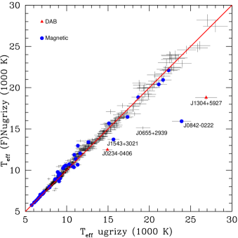
Figure 2: A comparison between the effective temperature derived from optical only data versus a combination of the UV and optical data for the DA white dwarfs in the 100 pc SDSS $\cap$ GALEX sample. Unusual objects, magnetic DAH and mixed composition DAB white dwarfs, are labeled with blue dots and red triangles, respectively.

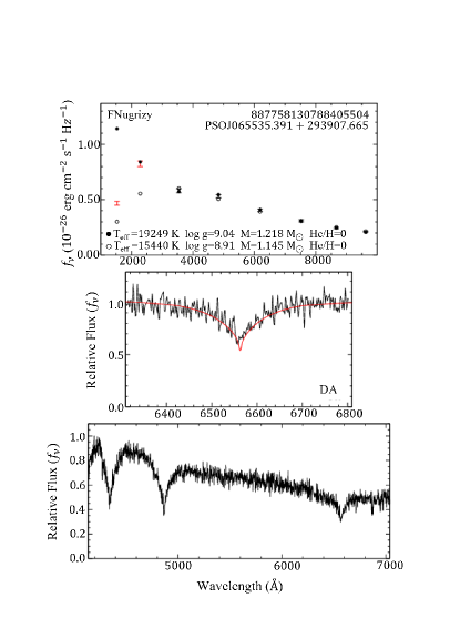
Figure 3: Model atmosphere fits to the DA white dwarf J0655+2939. The top panel shows the best-fitting H (filled dots) and He (open circles) atmosphere white dwarf models to the optical photometry (black error bars). The middle panel shows the observed spectrum (black line) along with the predicted spectrum (red line) based on the pure H atmosphere solution. The bottom panel shows a broader wavelength range.

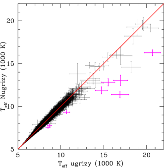
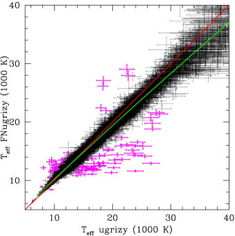
Figure 4: A comparison between the effective temperature derived from optical only data (SDSS $u$ and Pan-STARRS $grizy$) versus the optical + UV data for the DA white dwarfs in the SDSS footprint. The left panel shows objects with only NUV data, whereas the right panel includes objects with both FUV and NUV data. The 1:1 line is shown in red. The green line is the best-fitting polynomial to the data. The $3\sigma$ outliers are shown in magenta.

Figure 2 shows a comparison between the model fits using optical data only versus a combination of the optical + UV data for the DA white dwarfs in the 100 pc SDSS sample. Blue dots and red triangles mark the magnetic and DAB white dwarfs, respectively. The majority of the objects in this figure fall very close to the 1:1 line, shown in red, confirming that they are consistent with pure hydrogen atmosphere white dwarfs.

Excluding the five significant outliers labeled in the figure, the effective temperature and $\log{g}$ derived from the GALEX+optical data are slightly higher than the values obtained from the optical data only by $50^{+215}_{-71}$ K and $0.01^{+0.04}_{-0.01}$ dex, respectively. Hence, there are no major systematic differences between the best-fit parameters derived from optical only data and the optical + UV photometry. However, the addition of the GALEX FUV and NUV data helps improve the statistical errors in the model fits, especially for the hotter white dwarfs where the spectral energy distribution peaks in the UV. For example, for white dwarfs with $T_{\rm eff}<10000$ K, the statistical errors in optical + UV temperature estimates are on average better by a factor of 1.3 compared to the errors based on the optical data only, but they are better by a factor of 2.5 for $T_{\rm eff}>15000$ K.

The five significant outliers in Figure 2 all appear to be fainter than expected in the UV, and that is why their best-fitting temperatures based on the optical + UV model fits are cooler than those based on the optical data. These outliers include two DA white dwarfs with unusual atmospheric composition. J1304+5927 (GD 323, see Figure 1) and J0234$-$0406 (PSO J038.5646$-$04.1025). The latter was originally classified as a DA white dwarf based on a low-resolution spectrum obtained by Kilic et al. (2020). Higher signal-to-noise ratio follow-up spectroscopy by Gentile Fusillo et al. (2021) demonstrated that J0234$-$0406 is in fact a DABZ white dwarf that hosts a gaseous debris disk. Even though its spectral appearance is visually dominated by broad Balmer absorption lines, the atmosphere of J0234$-$0406 is actually dominated by helium, and that is why it is an outlier in Figure 2.

J0842$-$0222 (PSO J130.5623$-$02.3741) and J1543+3021 (PSO J235.8127+30.3595) are both strongly magnetic and massive white dwarfs with $M>1.1~{}M_{\odot}$ and unusual optical spectra. Schmidt et al. (1986) noted problems with fitting the UV and optical spectral energy distribution of the strongly magnetic white dwarf PG 1031+234 with a field stronger than 200 MG. They found that the IUE and optical/infrared fits cannot be reconciled and that there is no Balmer discontinuity in the spectrum of this object. They attribute this to the blanketing due to hydrogen lines being grossly different, and the addition of a strong opacity source (cyclotron absorption). GD 229 is another example of a magnetic white dwarf with inconsistent UV and optical temperature estimates (Green & Liebert, 1981). Out of the 51 magnetic white dwarfs shown in Figure 2, only J0842$-$0222 and J1543+3021 have significantly discrepant UV and optical temperatures. Hence, such inconsistencies seem to impact a fraction of the magnetic DA white dwarfs in the solar neighborhood.

Another outlier, J0655+2939 (PSO J103.8966+29.6527), is also a massive white dwarf with $M\sim 1.2~{}M_{\odot}$. We obtained follow-up optical spectroscopy of J0655+2939 using the KOSMOS spectrograph on the APO 3.5m telescope on UT 2023 Jan 28. We used the blue grism in the high slit position with a $2.05\arcsec$ slit, providing wavelength coverage from 4150 Å to 7050 Å and a resolution of 1.42 Å per pixel in the $2\times 2$ binned mode.

Figure 3 shows our model fits for J0655+2939. The top panel shows the best-fitting H (filled dots) and He (open circles) atmosphere white dwarf models to the optical photometry (black error bars). Note that the GALEX photometry (red error bars) are not used in these fits. The middle panel shows the observed spectrum (black line) along with the predicted spectrum (red line) based on the pure H atmosphere solution. The bottom panel shows the entire KOSMOS spectrum. We confirm J0655+2939 as a DA white dwarf. Even though its Balmer lines and the optical + NUV photometry agree with the pure H atmosphere solution, J0655+2939 is significantly fainter than expected in the GALEX FUV band. The source of this discrepancy is unclear, but the observed H$\alpha$ line core is also slightly shallower than expected based on the pure H atmosphere model.

4.2 The MWDD DA sample

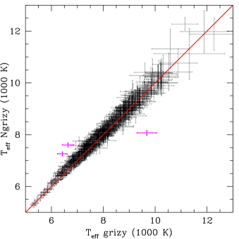
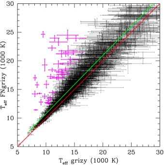
Figure 5: Same as Figure 4, but for the DA white dwarfs outside of the SDSS footprint.

Figure 6: Fits to the optical (left) and optical + UV (right) spectral energy distributions of two of the outliers in our DA white dwarf sample. The top panels show the fits for the double-lined spectroscopic binary WD 0037$-$006, and the bottom panels show the fits for a previously known DA + M dwarf binary.

The 100 pc SDSS DA white dwarf sample discussed in the previous section clearly demonstrates that 1) there are no large-scale systematic differences between the model fits using optical only data ($ugriz$) and a combination of optical + UV data, and 2) GALEX FUV and NUV data can be used to identify unusual DA white dwarfs with helium-rich atmospheres or strong magnetic fields. We now expand our study to the entire Montreal White Dwarf Database DA white dwarf sample in the Pan-STARRS $\cap$ GALEX footprint.

Figure 4 shows a comparison between the effective temperatures derived from optical and UV data for the DA white dwarfs in the SDSS footprint. The difference from Figure 2 is that the sample shown here extends beyond 100 pc, and therefore is corrected for reddening using the de-reddening procedure from Harris et al. (2006) and the GALEX extinction coefficients from Wall et al. (2019). The left panel includes objects with only NUV data, whereas the right panel includes objects with both FUV and NUV data. The red line shows the 1:1 line, and the green line is the best-fitting polynomial to the data. The magenta points mark the outliers that are $3\sigma$ away from both lines. The best-fitting polynomial takes the form

$$y=c_{2}x^{2}+c_{1}x+c_{0},$$ (1)

where y is the $T_{\rm eff}FNugrizy/1000$ and x is $T_{\rm eff}ugrizy/1000$. The coefficients are given in table LABEL:tab:coeff. The sample with the NUV data only (left panel) is limited mostly to white dwarfs with temperatures between 5000 and 12000 K. This is simply an observational bias; hotter white dwarfs would be brighter in the FUV, and therefore they would have been detected in both NUV and FUV bands.

A comparison between the model parameters obtained from $ugrizy$ and $Nugrizy$ (left panel) shows that there are no systematic differences between the two sets of fits. We find eight $3\sigma$ outliers based on this analysis, all very similar to the outliers shown in Figure 2 with UV flux deficits.

On the other hand, we do find a systematic trend in the temperature measurements from the fits using the GALEX FUV, NUV, SDSS $u$, and Pan-STARRS $grizy$ filters shown in the right panel. Here the best-fitting polynomial shows that the temperatures based on the optical + UV data are slightly underestimated compared to the temperatures obtained from the optical data only. The difference is $-180$ K at 15000 K, $-620$ K at 20000 K, and $-1670$ K at 30000 K. Note that the average temperature errors based on the optical data are 670, 970, and 1850 K at 15000, 20000, and 30000 K, respectively. Hence, the observed systematic shift in this figure is consistent with the optical constraints on the same systems within $1\sigma$. We identify 83 outliers $3\sigma$ away from both the 1:1 line and the best-fitting polynomial (red and green lines in the figure) including a number of UV-excess objects.

Figure 5 shows a similar comparison for the DA white dwarfs outside of the SDSS footprint. These do not have SDSS $u$-band measurements, hence our model fits are based on the Pan-STARRS $grizy$ and GALEX FUV and NUV bands. The left panel shows the model fits for the DA sample with only NUV data available. Here the 1:1 line provides an excellent match to the parameters obtained from both the optical and the optical + UV analysis. We identify only 3 outliers based on this subsample.

The right panel in Figure 5 reveals a systematic trend in the temperature measurements based on the GALEX FUV + NUV + $grizy$ data compared to the temperatures derived from the optical only data. The best-fitting polynomial takes the form of equation 1 where y is the $T_{\rm eff}FNgrizy/1000$ and x is $T_{\rm eff}grizy/1000$. The coefficients are given in table LABEL:tab:coeff. This trend is similar to the one seen for the SDSS sample (right panel in Figure 4) but it is in the opposite direction. The optical + UV analysis leads to temperatures that are slightly over-estimated compared to the analysis using the optical data only. The difference is +850, +950, and +1090 K at 15000, 20000, and 30000 K, respectively. The average temperature errors based on the optical data are 670, 2810, and 6040 K at 15000, 20000, and 30000 K, respectively. Again, the observed systematic trend is consistent with the results from the optical only analysis within $1\sigma$. We identify 41 outliers, all of which are UV-excess objects, based on this diagram.

Table 1: Coefficients for the best-fitting polynomials in figures 4 and 5.

Coefficient	Figure 4	Figure 5
$c_{0}$	0.82743420	0.48395959
$c_{1}$	0.94949536	1.02740975
$c_{2}$	-0.00109481	-0.00021316

Table 2: The list of outliers that were previously known to be unusual. The horizontal line separates the UV-deficit (top) and the UV-excess (bottom) objects.

Object	Gaia DR3 Source ID	Spectral Type	Reference
PSO J012.0395$-$01.4109	2530629365419780864	DA(He)	Kilic et al. (2020)
PSO J017.4701+18.0000	2785085218267094784	DA(He)	Kepler et al. (2015)
PSO J025.4732+07.7206	2571609886069150592	DAB	Kepler et al. (2015)
PSO J027.3938+24.0130	291186211300158592	DZA	Gentile Fusillo et al. (2017)
PSO J033.0221+06.7391	2521035817229538688	DA:H:	Kleinman et al. (2013)
PSO J038.5646$-$04.1025	2489275328645218560	DABZ	Gentile Fusillo et al. (2021)
PSO J055.6249+00.4048	3263696071424152704	DA+DB	Limoges & Bergeron (2010)
PSO J119.5813+35.7453	906772187229375104	DAH	Kleinman et al. (2013)
PSO J123.8841+21.9779	676473944873877248	DAB	Kleinman et al. (2013)
PSO J125.6983+12.0296	649304840753259520	DAH:	Kepler et al. (2015)
PSO J130.5623$-$02.3741	3072348715677121280	DAH?DBH?	Kilic et al. (2020)
PSO J131.8174+48.7057	1015028491488955776	DBH:	Kleinman et al. (2013)
PSO J132.3710+28.9556	705246450482748288	DAH	Kleinman et al. (2013)
PSO J132.6463+32.1345	706974637946866304	DABZ	Kong et al. (2019)
PSO J133.2881+58.7267	1037873899276147840	DABZ	Gentile Fusillo et al. (2019)
PSO J136.6362+08.1209	584319855260594560	DAH	Kleinman et al. (2013)
PSO J140.1791+04.8533	579476334742123904	DA:B:Z:	Kleinman et al. (2013)
PSO J140.7411+13.2557	594146225037566976	DABZ	Kepler et al. (2015)
PSO J143.7587+44.4946	815134799361707392	DAH:	Kepler et al. (2015)
PSO J144.9871+37.1739	799763528023185280	DAB	Kepler et al. (2015)
PSO J150.9846+05.6405	3873396705206744064	DAH	Kleinman et al. (2013)
PSO J154.6449+30.5584	742562844335742208	DAH	Kleinman et al. (2013)
PSO J179.9671+00.1309	3891115064506627840	DA(He)	Kilic et al. (2020)
PSO J182.5106+18.0931	3949977724441143552	DAB	Kepler et al. (2015)
PSO J196.1335+59.4594	1579147088331814144	DAB	Wesemael et al. (1993)
PSO J198.6769+06.5415	3729586288010410496	DA(He)	Kepler et al. (2015)
PSO J201.2108+29.5887	1462096958792720384	DA(He)	Kepler et al. (2016)
PSO J206.1217+21.0809	1249447115013660416	DABZ	Kleinman et al. (2013)
PSO J211.9610+30.1917	1453322271887656448	DA:H:	Kleinman et al. (2013)
PSO J218.8923+04.5738	3668901977825959040	DAX	Kepler et al. (2015)
PSO J223.2567+06.8724	1160931721694284416	DA:H:	Kleinman et al. (2013)
PSO J223.9933+18.2145	1188753901361576064	DA:H:	Kleinman et al. (2013)
PSO J234.3569+51.8575	1595298501827000960	DBA	Kleinman et al. (2013)
PSO J240.2518+04.7101	4425676551115360512	DAH	Kleinman et al. (2013)
PSO J261.1339+32.5709	1333808965722096000	DAH	Kepler et al. (2015)
PSO J341.2484+33.1715	1890785517284104960	DAH/DQ	Kepler et al. (2016)
PSO J356.5226+38.8938	1919346461391649152	DAH	Kleinman et al. (2013)
PSO J010.0954$-$00.3584	2542961560852591744	DA+DA	Napiwotzki et al. (2020)
PSO J042.5074$-$04.6175	5184589747536175104	DAH:	Kepler et al. (2016)
PSO J051.5805+13.5189	17709047809907584	DAH	Kilic et al. (2020)
PSO J063.1211$-$11.5012	3189613692364776576	DA+DA	Napiwotzki et al. (2020)
PSO J065.0980+47.5929	257933852944165120	DAB	Verbeek et al. (2012)
PSO J094.8914+55.6121	997854527884948992	DAO	Gianninas et al. (2011)
PSO J109.2922+74.0109	1112171030998592256	DAM	Marsh & Duck (1996)
PSO J122.8223+57.4396	1035077806847142144	DAM	Rebassa-Mansergas et al. (2016)
PSO J123.9537+47.6772	931238043230275968	DAM	Farihi et al. (2010)
PSO J140.2868+13.0199	594229753561550208	DAH	Kleinman et al. (2013)
PSO J173.7025+46.8094	785521450828261632	DD?	Bédard et al. (2017)
PSO J182.0967+06.1655	3895444662122848512	DAM	Rebassa-Mansergas et al. (2016)
PSO J224.1602+10.6747	1180256944222072704	DAM	Rebassa-Mansergas et al. (2016)
PSO J337.4922+30.4024	1900545847646195840	DAM?	Rebassa-Mansergas et al. (2019)
PSO J344.9451+16.4879	2828888597582293760	DAM	Farihi et al. (2010)

In total we identify 135 outliers based on this analysis. Because the full width at half-maximum of the GALEX point spread function is about 5 arcsec (Morrissey et al., 2007), blending and contamination from background sources is an issue. We checked the Pan-STARRS stacked images for each of these outliers to identify nearby sources that could impact GALEX, SDSS, or Pan-STARRS photometry measurements. We found that 24 of these outliers were likely impacted by blending sources, reducing the final sample size to 111 outliers.

Table LABEL:outknown presents the list of 52 outliers that were previously known to be unusual. This list includes four objects that are confirmed or suspected to be double white dwarfs (PSO J010.0954$-$00.3584, J055.6249+00.4048, J063.1211$-$11.5012, and J173.7025+46.8094), 20 confirmed or suspected magnetic white dwarfs, seven DA + M dwarf systems, and 21 objects with an unusual atmospheric composition (DAB etc).

Figure 6 shows the spectral energy distributions for two of these outliers. The top panels show the fits to the optical and UV + optical spectral energy distributions of the previously known double-lined spectroscopy binary WD 0037$-$006 (Napiwotzki et al., 2020). Under the assumption of a single star, the Pan-STARRS photometry for WD 0037$-$006 indicates $T_{\rm eff}=10330\pm 380$ K and $\log{g}=7.36\pm 0.05$. Adding the GALEX FUV and NUV data, the best-fitting solution significantly changes to $T_{\rm eff}=12590\pm 100$ K and $\log{g}=7.63\pm 0.01$. In addition, this solution has problems matching the entire spectral energy distribution, indicating that there is likely a cooler companion contributing significant flux. This figure demonstrates that double-lined spectroscopic binaries with significant temperature differences between the primary and the secondary star could be identified based on an analysis similar to the one presented here. A similar and complementary method for identifying double-lined spectroscopic binaries was pioneered by Bédard et al. (2017), which use optical photometry and spectroscopy to identify systems with inconsistent photometric and spectroscopic solutions.

The bottom panels in Figure 6 show the fits to a previously confirmed DA + M dwarf system in our sample (Rebassa-Mansergas et al., 2016). Here the optical data is clearly at odds with a single DA white dwarf, and GALEX FUV and NUV data reveal UV-excess from a hotter white dwarf. The analysis using $FNugrizy$ photometry confirms excess emission in the Pan-STARRS $zy$-bands, consistent with an M dwarf companion.

Table 3: Newly identified outliers among the DA white dwarf population with GALEX data. The horizontal line separates the UV-deficit (top) and the UV-excess (bottom) objects.

Object	Gaia DR3 Source ID	Optical	Optical + UV	Spectral	Reference	Notes
		$T_{\rm eff}$ (K)	$T_{\rm eff}$ (K)	Type
PSO J018.6848+35.4095	321093335597030400	15369 $\pm$ 678	11872 $\pm$ 223	DA	Gentile Fusillo et al. (2015)	DA(He) LAMOST
PSO J032.2011+12.2256	73623921366683008	27516 $\pm$ 1379	21586 $\pm$ 476	DA	Kleinman et al. (2013)
PSO J043.8655+02.6202	1559111783825792	8685 $\pm$ 254	7788 $\pm$ 117	DA	Kilic et al. (2020)
PSO J056.0479+15.1626	42871199614383616	8503 $\pm$ 241	7548 $\pm$ 90	DA	Andrews et al. (2015)
PSO J103.8966+29.6527	887758130788405504	19249 $\pm$ 849	15130 $\pm$ 168	DA	Kilic et al. (2020)	massive
PSO J130.7484+10.6677	598412403168328960	15748 $\pm$ 731	12139 $\pm$ 293	DAZ	Kepler et al. (2015)	DZA SDSS
PSO J132.2963+14.4454	608922974120358784	19793 $\pm$ 1038	11354 $\pm$ 226	DA	Gentile Fusillo et al. (2019)
PSO J139.0499+34.9872	714469355877947136	23646 $\pm$ 1571	14667 $\pm$ 545	DA	Kleinman et al. (2013)	massive
PSO J151.1401+40.2417	803693216941983232	13881 $\pm$ 797	10816 $\pm$ 188	DA	Kepler et al. (2015)	DA(He) SDSS
PSO J158.8293+27.2510	728222390915647872	17876 $\pm$ 998	12484 $\pm$ 307	DA	Gentile Fusillo et al. (2019)
PSO J159.5929+37.3533	751930335511863040	14891 $\pm$ 628	12383 $\pm$ 194	DA:DC:	Kleinman et al. (2013)	DAB SDSS
PSO J163.5943$-$02.7860	3801901270848297600	25209 $\pm$ 1429	15858 $\pm$ 522	DA	Croom et al. (2001)	massive
PSO J172.6518$-$00.3655	3797201653208863360	15198 $\pm$ 761	11058 $\pm$ 264	DA:Z	Kleinman et al. (2013)	DZA SDSS
PSO J180.6015+40.5822	4034928775942285184	16551 $\pm$ 835	11880 $\pm$ 377	DA	Kleinman et al. (2013)	DC: SDSS
PSO J196.7725+49.1045	1554826818838504576	14573 $\pm$ 736	11689 $\pm$ 225	DA:	Kleinman et al. (2013)	DA(He) SDSS
PSO J213.8277+31.9308	1477633195532154752	16960 $\pm$ 829	13040 $\pm$ 608	DAZ	Gentile Fusillo et al. (2019)	DZA SDSS
PSO J215.2971+38.9912	1484931581918492544	17743 $\pm$ 873	14159 $\pm$ 483	DA:	Kleinman et al. (2013)	DC: SDSS
PSO J231.8495+06.7581	1162614902197098624	16792 $\pm$ 1013	12897 $\pm$ 411	DA	Carter et al. (2013)	massive
PSO J249.3471+53.9644	1426634650780861184	16315 $\pm$ 761	12321 $\pm$ 257	DAZ	Kepler et al. (2016)
PSO J309.1036+77.8178	2290767158609770240	28040 $\pm$ 1427	21372 $\pm$ 486	DA	Bédard et al. (2020)
PSO J324.1725+01.0846	2688259922223271296	16404 $\pm$ 937	12078 $\pm$ 389	DA	Vidrih et al. (2007)
PSO J338.5445+25.1894	1877374842678152704	16838 $\pm$ 892	11787 $\pm$ 266	DA	Gentile Fusillo et al. (2019)	DA(He) SDSS
PSO J342.5363+22.7580	2836800855054851456	26580 $\pm$ 1279	20752 $\pm$ 605	DA	Bédard et al. (2020)
PSO J348.7601+22.1674	2838958711048617856	26837 $\pm$ 1327	19773 $\pm$ 571	DA	Kleinman et al. (2013)
PSO J003.9449$-$30.1015	2320237751020937728	9768 $\pm$ 375	13816 $\pm$ 408	DA	Vennes et al. (2002)
PSO J009.0492$-$17.5443	2364297204875140224	13479 $\pm$ 1408	21203 $\pm$ 437	DA	Gianninas et al. (2011)
PSO J015.0435$-$28.1077	5033974938207807488	13023 $\pm$ 1105	17630 $\pm$ 337	DA	Croom et al. (2004)
PSO J019.3103+24.6726	294062563782633216	12160 $\pm$ 1007	17090 $\pm$ 490	DA	Kleinman et al. (2013)
PSO J021.9568+73.4798	535482641132742400	6422 $\pm$ 190	7259 $\pm$ 75	DA	Limoges et al. (2015)
PSO J023.0575$-$28.1766	5035296654263954304	12745 $\pm$ 931	17999 $\pm$ 527	DA	Croom et al. (2004)
PSO J029.9572$-$27.8589	5024390701506507648	11176 $\pm$ 562	14449 $\pm$ 337	DA	Croom et al. (2004)
PSO J041.4724$-$12.7058	5158731712247303040	9493 $\pm$ 307	24634 $\pm$ 504	DA	Kilkenny et al. (2016)	DAM?
PSO J051.6792+69.4045	494644717692834944	13855 $\pm$ 1393	19565 $\pm$ 343	DA	Gianninas et al. (2011)
PSO J052.0294+52.9603	443375555640546944	10729 $\pm$ 467	13492 $\pm$ 282	DA	Verbeek et al. (2012)
PSO J052.2834+52.7335	443274778529615232	10363 $\pm$ 382	12680 $\pm$ 249	DA	Verbeek et al. (2012)
PSO J102.2271+38.4434	944388335442133888	13883 $\pm$ 1606	21741 $\pm$ 901	DA	Kleinman et al. (2013)
PSO J125.7399+57.8364	1034975243028553600	18178 $\pm$ 2420	31076 $\pm$ 1012	DA	Bédard et al. (2020)
PSO J143.4929+17.7146	632864633657062400	13811 $\pm$ 1864	24486 $\pm$ 883	DA	Bédard et al. (2020)	DAM?
PSO J143.5436+22.4702	644043544469790720	14268 $\pm$ 1613	20245 $\pm$ 465	DA	Kleinman et al. (2013)	DAM?
PSO J146.2852+62.7948	1063508669280315776	9623 $\pm$ 370	12604 $\pm$ 502	DA	Kleinman et al. (2013)	DAM?
PSO J149.4751+85.4946	1147853241336105344	28499 $\pm$ 4417	50953 $\pm$ 4975	DA	Gianninas et al. (2011)
PSO J150.3866+01.5162	3835962526168788608	22704 $\pm$ 1127	27966 $\pm$ 821	DA	Kepler et al. (2015)
PSO J167.1417+31.8979	757803896562843392	14778 $\pm$ 1760	21458 $\pm$ 382	DA	Gianninas et al. (2011)
PSO J192.2894+24.0266	3957635410611476096	10266 $\pm$ 381	12108 $\pm$ 291	DA	Kleinman et al. (2013)
PSO J200.6206+01.0147	3688065808367722368	9383 $\pm$ 291	11459 $\pm$ 371	DA	Croom et al. (2004)	DAM?
PSO J211.4189+74.6498	1712016196599965312	8237 $\pm$ 305	11420 $\pm$ 77	DA	Mickaelian (2008)	resolved DAM
PSO J218.2047+01.7710	3655853106971493760	10341 $\pm$ 329	11793 $\pm$ 97	DA	Kleinman et al. (2013)
PSO J221.4238+41.2449	1489712503290614912	9786 $\pm$ 396	19274 $\pm$ 1067	DA	Bédard et al. (2020)	DAM?
PSO J223.4269+46.9171	1590342178286505216	12174 $\pm$ 851	19440 $\pm$ 593	DA	Kleinman et al. (2013)
PSO J240.6992+43.8100	1384551977098980608	10070 $\pm$ 352	12113 $\pm$ 369	DA	Kleinman et al. (2013)	resolved DAM?
PSO J240.8660+19.6618	1203265358904378880	10085 $\pm$ 401	15880 $\pm$ 632	DA	Kleinman et al. (2013)	DAM?
PSO J244.6129+20.5911	1202035422006406400	9808 $\pm$ 394	12191 $\pm$ 410	DA	Kleinman et al. (2013)	resolved DAM?
PSO J259.6449+01.9471	4387171623850187648	10215 $\pm$ 438	12685 $\pm$ 84	DA	McCleery et al. (2020)
PSO J263.1394+32.8366	4601788317833882240	9790 $\pm$ 353	11747 $\pm$ 336	DA	Kepler et al. (2015)	DAM?
PSO J276.0344+35.2718	2095603539740855296	11063 $\pm$ 653	22229 $\pm$ 415	DA	Mickaelian (2008)	DAM?
PSO J334.7157$-$29.4534	6615258025441899776	10838 $\pm$ 624	17254 $\pm$ 376	DA	Croom et al. (2004)	DAM?
PSO J346.5586$-$28.0099	6606686198432918656	11516 $\pm$ 779	23961 $\pm$ 485	DA	Croom et al. (2004)	resolved DAM?
PSO J352.1333$-$30.0610	2329285662270302976	12190 $\pm$ 1555	23284 $\pm$ 616	DA	Vennes et al. (2002)
PSO J355.9551+38.5749	1919325605029184000	10573 $\pm$ 344	12004 $\pm$ 78	DA	Kleinman et al. (2013)

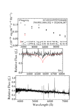
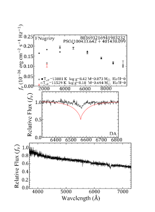
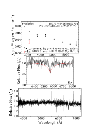
Figure 7: Model atmosphere fits to three DA white dwarfs with UV flux deficits. The top panels show the best-fitting H (filled dots) and He (open circles) atmosphere white dwarf models to the optical photometry (black error bars). The middle panels show the observed spectrum (black line) along with the predicted spectrum (red line) based on the pure H atmosphere solution. The bottom panels show a broader wavelength range. GALEX FUV and NUV data clearly favor the He-dominated atmosphere solutions, which are also confirmed by the relatively weak Balmer lines in their spectra.

Figure 8: Fits to the optical (left) and optical + UV (right) spectral energy distributions of three of the newly identified UV excess sources in our DA white dwarf sample. The inconsistent temperature estimates from the optical and UV photometry and optical spectroscopy indicate that they may be double white dwarfs.

Table LABEL:outnew presents the list of 59 newly identified outliers among the DA white dwarfs with GALEX data; 24 of them show flux deficits in the UV (their optical + UV temperatures are lower than the temperatures based on the optical data only), and 35 are UV-excess objects. We include the spectral types from the literature for each source.

Even though the 24 UV-deficit objects (shown in the top half of the table) are classified as DA in the literature, our analysis indicates that they are unusual. For example, re-inspecting the SDSS spectra for three of the sources classified as DAZ in the literature, we find that the Ca H and K lines are actually stronger than the Balmer lines, indicating that they are in fact DZA white dwarfs.

Similarly, re-inspecting the SDSS and LAMOST spectra for four of these sources (PSO J018.6848+35.4095, J151.1401+40.2417, J196.7725+49.1045, and J338.5445+25.1894), we find that their Balmer lines are much weaker than expected for these relatively warm white dwarfs with $T_{\rm eff}>10,000$ K. Figure 7 shows the model fits to three of these objects based on the optical photometry. All three stars are significantly fainter than expected in the FUV and NUV bands compared to the pure H atmosphere models. The UV photometry and the weak Balmer lines indicate that these stars are likely DA(He) white dwarfs with helium dominated atmospheres.

The newly identified UV excess sample likely includes many binaries, including white dwarf + main-sequence and double white dwarf systems. We classify 14 of these systems as likely DA + M dwarfs based on their spectral energy distributions, which are dominated by the white dwarf in the UV and by a redder source in the Pan-STARRS $zy$ bands. Four of these DA + M dwarf systems are also resolved in the Pan-STARRS $zy$ band stacked images, but the resolved companions are not included in the Pan-STARRS photometric catalog. However, one of these resolved systems is confirmed to be a physical binary through Gaia astrometry. Both components of PSO J211.4189+74.6498 are detected in Gaia with source IDs Gaia DR3 1712016196599965312 and 1712016196599171840.

Figure 8 shows the fits to the optical and optical + UV spectral energy distributions for three of the newly identified UV excess sources that may be double white dwarfs. There are small but significant temperature discrepancies between the photometric solutions relying on optical and optical + UV data and also the optical spectroscopy. For example, for PSO J218.2047+01.7710 the model fits to the optical photometry give $T_{\rm eff}=10341\pm 329$ K and $\log{g}=7.51\pm 0.05$, while the fits to the optical + UV photometry give $T_{\rm eff}=11793\pm 98$ K and $\log{g}=7.74\pm 0.02$. Fitting the normalized Balmer line profiles, Tremblay et al. (2011) obtained $T_{\rm eff}=11360\pm 120$ K and $\log{g}=8.19\pm 0.06$ for the same star. The inconsistent $\log{g}$ estimates can be explained if the photometry is contaminated by a companion (see also Bédard et al., 2017), and the small temperature differences between the different solutions favor a white dwarf companion rather than a cool, late-type M dwarf star. Follow-up spectroscopy of these three systems, as well as the rest of the UV excess sample would be helpful for constraining the nature of these objects and identifying additional double white dwarf binaries.

5 Results from UV Magnitude Comparison

The optical/UV temperature comparison method presented in the previous section provides an excellent method to identify sources with grossly different temperatures. However, it may miss some sources with unusual UV fluxes. Those model fits rely on three ($gri$) to six ($ugrizy$) optical filters versus one or two GALEX UV filters, hence the UV data have a lesser weight in constraining the temperatures.

To search for additional outliers that were potentially missed by the temperature comparison method, here we use model fits to the optical photometry plus Gaia parallaxes to predict the brightness of each star in the GALEX filters, and search for significant outliers using FUV and NUV data. To obtain the best constraints on the predicted FUV and NUV brightnesses of each source, we further require our stars to have photometry in the SDSS $u$ filter as well as all of the Pan-STARRS filters. Our final magnitude comparison sample contains 10049 DA white dwarfs with photometry in at least one of the GALEX filters, the SDSS $u$, and the Pan-STARRS $grizy$ filters.

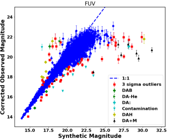
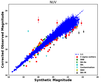
Figure 9: Comparison between observed and model FUV (left) and NUV (right) magnitudes. The blue dashed line is the 1:1 correlation. The green diamonds are previously known DAB white dwarfs, the green triangles are previously known DA-He white dwarfs, the cyan diamonds are white dwarfs with uncertain classifications, the cyan triangles are objects with contaminated photometry, and the yellow diamonds are previously known magnetic white dwarfs. Previously unknown 3$\sigma$ outliers are plotted as red squares.

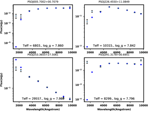
Figure 10: Spectral energy distributions of four newly identified outliers in the magnitude comparison sample. The filled dots are the model fluxes and the error bars are the observed photometry.

Figure 9 shows a comparison of the observed and predicted FUV (left) and NUV (right panel) magnitudes of the 10049 DA white dwarfs in our magnitude comparison sample. The blue dashed line is the 1:1 correlation between observed and model magnitudes. The green diamonds are previously known DAB white dwarfs while the green triangles are DA white dwarfs that have significant amounts of helium in their atmospheres, making the use of pure hydrogen atmosphere models inappropriate. The yellow diamonds are previously known magnetic white dwarfs and the black triangles are previously known DA + M dwarf systems. The blue diamonds are white dwarfs with uncertain (e.g., DA:) classifications.

As with the temperature comparison sample, blending and contamination from background sources is an issue for some sources. We checked the Pan-STARRS stacked images for each of these outliers to identify nearby sources that could impact GALEX, SDSS, or Pan-STARRS photometry measurements. The outliers that were affected by contamination are marked by blue triangles in Figure 9. The red squares are 30 newly identified $3\sigma$ outliers. Table LABEL:magnew presents this list along with their photometric and spectroscopic temperatures based on the optical data.

Figure 10 displays the spectral energy distributions for four of these outliers. Outliers with UV excesses, such as PSO J226.4550+11.0849 shown in the top right panel of Figure 10, are likely binaries. Outliers with UV deficits, such as PSO J253.3655+27.5061 shown in the bottom left of Figure 10, do not fit the expectations from pure hydrogen atmosphere models in the UV. Their atmospheres might be dominated by helium or might contain metals, making the use of pure hydrogen models inappropriate. Alternatively, they could also be magnetic. Further observations are needed to confirm the nature of these UV excess and UV deficit objects.

Table 4: Additional outliers identified through a comparison of the observed and predicted UV magnitudes.

Object	Gaia DR3 Source ID	Photometric	Spectroscopic	Spectral	Reference	Notes
		$T_{\rm eff}$ (K)	$T_{\rm eff}$ (K)	Type
PSO J001.0830+23.8334	2849729771768028544	27453	34738	DA	Kepler et al. (2016)
PSO J004.9372+33.6842	2864011530163554816	7513	8982	DA	Kepler et al. (2016)
PSO J005.7002+00.7079	2546893650655427840	6803	6992	DA	Kleinman et al. (2013)	DAM?
PSO J021.8549+27.6214	296372465914661248	6823	6723	DA	Kepler et al. (2016)
PSO J056.0308-05.2121	3244802712151826048	10331	12371	DA	Kleinman et al. (2013)	DAM?
PSO J118.9063+21.1283	673549759340742272	9270	9941	DA	Kleinman et al. (2013)	DAM?
PSO J126.3419+17.4310	662102679359467648	7867	7838	DA	Kleinman et al. (2013)
PSO J137.9380+35.5266	714377928911156992	14027	19527	DA	Kleinman et al. (2013)
PSO J149.4951+57.6078	1046386971133757184	10292	11288	DA	Kleinman et al. (2013)	DAM?
PSO J152.4806+00.1622	3831830527112439936	10569	10513	DA	Kleinman et al. (2013)
PSO J176.3500+24.1592	4004972723377902592	7188	7403	DA	Kepler et al. (2016)
PSO J189.9978+33.1080	1514768341766532992	10348	10957	DA	Kleinman et al. (2013)	DAM?
PSO J204.9827+60.1751	1662524184641472640	7888	9463	DA	Kleinman et al. (2013)
PSO J205.8897+23.2339	1443624343108905216	9516	10373	DA	Kleinman et al. (2013)
PSO J210.9347+37.1660	1483513830393895680	8703	11040	DA	Kepler et al. (2015)	DAM?
PSO J213.9910+62.5129	1666750569898974208	9593	10114	DA	Kleinman et al. (2013)
PSO J226.4550+11.0849	1180520345976350208	10315	11354	DA	Kleinman et al. (2013)
PSO J226.6089+06.6459	1160300056558791168	9500	10670	DA	Farihi et al. (2012)
PSO J227.2923+37.1129	1292306146987734784	8264	8526	DA	Kepler et al. (2015)
PSO J244.4451+40.3379	1380686815769537920	7600	13013	DA	Kepler et al. (2015)	DAM?
PSO J248.9274+26.3827	1304383217063475968	30346	34544	DA	Kleinman et al. (2013)
PSO J249.2986+12.8853	4459617994029737216	7824	7904	DA	Kepler et al. (2015)	DAM?
PSO J250.5693+22.9411	1299405148103896832	11188	12763	DA	Kleinman et al. (2013)
PSO J251.3785+41.0348	1356243233471452288	7884	8068	DA	Kepler et al. (2015)
PSO J253.3655+27.5061	1306991499163308160	29557	30472	DA	Kleinman et al. (2013)
PSO J328.6059-00.6697	2680152673235328768	17608	20257	DA	Kleinman et al. (2013)
PSO J331.0859+24.2120	1795394701659196032	6847	6873	DA	Kepler et al. (2015)	DAM?
PSO J341.3178+00.6951	2653703714870987648	8299	9611	DA	Kleinman et al. (2013)	DAM?
PSO J349.8567+07.6224	2664938112366990080	7394	8519	DA	Kepler et al. (2016)
PSO J358.8416+16.8000	2773308246143281920	7149	7066	DA	Kepler et al. (2016)

6 Conclusions

We analyzed the UV to optical spectral energy distributions of 14001 DA white dwarfs from the Montreal White Dwarf Database, taking advantage of the GALEX FUV and NUV data and Gaia DR3 parallaxes. Using the 100 pc sample where extinction is negligible, we demonstrated that there are no major systematic differences between the best-fit parameters derived from optical only data and the optical + UV photometry. The effective temperatures derived from optical and UV + optical data differ by only $50^{+215}_{-71}$ K. The addition of GALEX FUV and NUV data in the model atmosphere analysis helps improve the statistical errors in the fits, especially for hot white dwarfs.

We used two different methods to identify UV excess or UV deficit objects. In the first method, we compared the temperatures obtained from fitting the optical data with those obtained from fitting optical + UV data. We identified 111 significant outliers with this method, including 52 outliers that were previously known to be unusual. These include DA white dwarfs with helium dominated atmospheres, magnetic white dwarfs, double white dwarfs, and white dwarf + M dwarf systems. Out of the 59 newly identified systems, 35 are UV excess and 24 are UV deficit objects. In the second method, we used the optical photometry to predict the FUV and NUV magnitudes for each source, and classified sources with $3\sigma$ discrepant FUV and/or NUV photometry as outliers. Using this method, we identified 30 additional outliers.

Combining these two methods, our final sample includes 89 newly identified outliers. The nature of these outliers cannot be constrained by our analysis alone. Many of the UV excess objects are likely binaries, including double degenerates and white dwarfs with late-type stellar companions. Follow-up spectroscopy and infrared observations of these outliers would help constrain their nature.

There are several current and upcoming surveys that are specifically targeting large numbers of white dwarfs spectroscopically. For example, the Dark Energy Spectroscopic Instrument Data Release 1 is expected to contain spectra for over 47000 white dwarf candidates (Manser et al., 2023). DA white dwarfs make up the majority of the white dwarf population. Hence, the number of spectroscopically confirmed DA white dwarfs will increase significantly in the near future. The Ultraviolet Transient Astronomy Satellite (ULTRASAT, Ben-Ami et al., 2022) will perform an all-sky survey during the first 6 months of the mission to a limiting magnitude of 23 to 23.5 in its 230-290 nm NUV passband. This survey will be about an order of magnitude deeper than GALEX. Future analysis of these larger DA white dwarf samples with GALEX FUV/NUV or ULTRASAT NUV data would provide an excellent opportunity to identify unusual objects among the DA white dwarf population.

Data availability

The data underlying this article are available in the MWDD at http://www.montrealwhitedwarfdatabase.org and also from the corresponding author upon reasonable request.

References

- Andrews et al. (2015) Andrews J. J., Agüeros M. A., Gianninas A., Kilic M., Dhital S., Anderson S. F., 2015, ApJ, 815, 63
- Bailer-Jones et al. (2021) Bailer-Jones C. A. L., Rybizki J., Fouesneau M., Demleitner M., Andrae R., 2021, AJ, 161, 147
- Bédard et al. (2017) Bédard A., Bergeron P., Fontaine G., 2017, ApJ, 848, 11
- Bédard et al. (2020) Bédard A., Bergeron P., Brassard P., Fontaine G., 2020, ApJ, 901, 93
- Ben-Ami et al. (2022) Ben-Ami S., et al., 2022, in den Herder J.-W. A., Nikzad S., Nakazawa K., eds, Society of Photo-Optical Instrumentation Engineers (SPIE) Conference Series Vol. 12181, Space Telescopes and Instrumentation 2022: Ultraviolet to Gamma Ray. p. 1218105 (arXiv:2208.00159), doi:10.1117/12.2629850
- Bergeron et al. (2019) Bergeron P., Dufour P., Fontaine G., Coutu S., Blouin S., Genest-Beaulieu C., Bédard A., Rolland B., 2019, ApJ, 876, 67
- Bianchi et al. (2017) Bianchi L., Shiao B., Thilker D., 2017, ApJS, 230, 24
- Camarota & Holberg (2014) Camarota L., Holberg J. B., 2014, MNRAS, 438, 3111
- Carter et al. (2013) Carter P. J., et al., 2013, MNRAS, 429, 2143
- Croom et al. (2001) Croom S. M., Smith R. J., Boyle B. J., Shanks T., Loaring N. S., Miller L., Lewis I. J., 2001, MNRAS, 322, L29
- Croom et al. (2004) Croom S. M., Smith R. J., Boyle B. J., Shanks T., Miller L., Outram P. J., Loaring N. S., 2004, MNRAS, 349, 1397
- Dufour et al. (2017) Dufour P., Blouin S., Coutu S., Fortin-Archambault M., Thibeault C., Bergeron P., Fontaine G., 2017, in Tremblay P. E., Gaensicke B., Marsh T., eds, Astronomical Society of the Pacific Conference Series Vol. 509, 20th European White Dwarf Workshop. p. 3 (arXiv:1610.00986)
- Eisenstein et al. (2006) Eisenstein D. J., et al., 2006, ApJS, 167, 40
- Farihi et al. (2010) Farihi J., Hoard D. W., Wachter S., 2010, ApJS, 190, 275
- Farihi et al. (2012) Farihi J., Gänsicke B. T., Steele P. R., Girven J., Burleigh M. R., Breedt E., Koester D., 2012, MNRAS, 421, 1635
- Genest-Beaulieu & Bergeron (2019) Genest-Beaulieu C., Bergeron P., 2019, ApJ, 882, 106
- Gentile Fusillo et al. (2015) Gentile Fusillo N. P., et al., 2015, MNRAS, 452, 765
- Gentile Fusillo et al. (2017) Gentile Fusillo N. P., Gänsicke B. T., Farihi J., Koester D., Schreiber M. R., Pala A. F., 2017, MNRAS, 468, 971
- Gentile Fusillo et al. (2019) Gentile Fusillo N. P., et al., 2019, MNRAS, 482, 4570
- Gentile Fusillo et al. (2021) Gentile Fusillo N. P., et al., 2021, MNRAS, 504, 2707
- Gianninas et al. (2011) Gianninas A., Bergeron P., Ruiz M. T., 2011, ApJ, 743, 138
- Green & Liebert (1981) Green R. F., Liebert J., 1981, PASP, 93, 105
- Harris et al. (2006) Harris H. C., et al., 2006, AJ, 131, 571
- Kepler et al. (2015) Kepler S. O., et al., 2015, MNRAS, 446, 4078
- Kepler et al. (2016) Kepler S. O., et al., 2016, MNRAS, 455, 3413
- Kilic et al. (2020) Kilic M., Bergeron P., Kosakowski A., Brown W. R., Agüeros M. A., Blouin S., 2020, ApJ, 898, 84
- Kilkenny et al. (2016) Kilkenny D., Worters H. L., O’Donoghue D., Koen C., Koen T., Hambly N., MacGillivray H., Stobie R. S., 2016, MNRAS, 459, 4343
- Kleinman et al. (2013) Kleinman S. J., et al., 2013, ApJS, 204, 5
- Kong et al. (2019) Kong X., Luo A. L., Li X.-R., 2019, Research in Astronomy and Astrophysics, 19, 088
- Kowalski & Saumon (2006) Kowalski P. M., Saumon D., 2006, ApJ, 651, L137
- Lajoie & Bergeron (2007) Lajoie C. P., Bergeron P., 2007, ApJ, 667, 1126
- Limoges & Bergeron (2010) Limoges M. M., Bergeron P., 2010, ApJ, 714, 1037
- Limoges et al. (2015) Limoges M. M., Bergeron P., Lépine S., 2015, ApJS, 219, 19
- Magnier et al. (2013) Magnier E. A., et al., 2013, ApJS, 205, 20
- Manser et al. (2023) Manser C. J., et al., 2023, MNRAS,
- Marsh & Duck (1996) Marsh T. R., Duck S. R., 1996, MNRAS, 278, 565
- Martin et al. (2005) Martin D. C., et al., 2005, ApJ, 619, L1
- McCleery et al. (2020) McCleery J., et al., 2020, MNRAS, 499, 1890
- Mickaelian (2008) Mickaelian A. M., 2008, AJ, 136, 946
- Morrissey et al. (2005) Morrissey P., et al., 2005, ApJ, 619, L7
- Morrissey et al. (2007) Morrissey P., et al., 2007, ApJS, 173, 682
- Napiwotzki et al. (2020) Napiwotzki R., et al., 2020, A&A, 638, A131
- Press et al. (1986) Press W. H., Flannery B. P., Teukolsky S. A., 1986, Numerical recipes. The art of scientific computing
- Rebassa-Mansergas et al. (2016) Rebassa-Mansergas A., et al., 2016, MNRAS, 463, 1137
- Rebassa-Mansergas et al. (2019) Rebassa-Mansergas A., Toonen S., Korol V., Torres S., 2019, MNRAS, 482, 3656
- Schmidt et al. (1986) Schmidt G. D., West S. C., Liebert J., Green R. F., Stockman H. S., 1986, ApJ, 309, 218
- Tremblay et al. (2011) Tremblay P. E., Bergeron P., Gianninas A., 2011, ApJ, 730, 128
- Vennes et al. (2002) Vennes S., Smith R. J., Boyle B. J., Croom S. M., Kawka A., Shanks T., Miller L., Loaring N., 2002, MNRAS, 335, 673
- Verbeek et al. (2012) Verbeek K., et al., 2012, MNRAS, 426, 1235
- Vidrih et al. (2007) Vidrih S., et al., 2007, MNRAS, 382, 515
- Wall et al. (2019) Wall R. E., Kilic M., Bergeron P., Rolland B., Genest-Beaulieu C., Gianninas A., 2019, MNRAS, 489, 5046
- Wesemael et al. (1993) Wesemael F., Greenstein J. L., Liebert J., Lamontagne R., Fontaine G., Bergeron P., Glaspey J. W., 1993, PASP, 105, 761