Causal Discovery using Bayesian Model Selection

Abstract

With only observational data on two variables, and without other assumptions, it is not possible to infer which one causes the other. Much of the causal literature has focused on guaranteeing identifiability of causal direction in statistical models for datasets where strong assumptions hold, such as additive noise or restrictions on parameter count. These methods are then subsequently tested on realistic datasets, most of which violate their assumptions. Building on previous attempts, we show how to use causal assumptions within the Bayesian framework. This allows us to specify models with realistic assumptions, while also encoding independent causal mechanisms, leading to an asymmetry between the causal directions. Identifying causal direction then becomes a Bayesian model selection problem. We analyse why Bayesian model selection works for known identifiable cases and flexible model classes, while also providing correctness guarantees about its behaviour. To demonstrate our approach, we construct a Bayesian non-parametric model that can flexibly model the joint. We then outperform previous methods on a wide range of benchmark datasets with varying data generating assumptions showing the usefulness of our method.

1 Introduction

Many fields use statistical models to predict the response to actions (interventions), e.g. health outcomes after treatment. Such predictions can not be made based on correlations gained from purely observational data, but require access to causal structure [41]. In machine learning, causal structure also helps in many prediction tasks ranging from domain adaptation [57], robustness [4], and generalisation [46]. Without further assumptions, only conditional independencies can be inferred from observational data, which do not even distinguish simple causal structures, like $X\!\rightarrow\!Y$ and $Y\!\rightarrow\!X$. In this paper, we aim to identify causal direction from observational data in the bivariate case.

Much of the causal literature assumes restrictions on a model, which when they match reality, allow strong guarantees of causal identifiability. For example, data generated by non-linear additive noise models cannot be modelled equally well in the anticausal direction, which allows causality to be identified [25]. The usefulness of a method in more general circumstances is verified empirically on benchmark datasets where the ground-truth causal structure is known. These include datasets where the restricted models are hampered in their performance as they don’t fit the dataset optimally due to misspecification, while causal identifiability is also not guaranteed. The goal of our work, is to investigate whether causality can be identified in flexible models that minimise misspecification, even if we lose strict guarantees of identifiability.

We replace hard restrictions on models with softer ones encoded by Bayesian priors. Each causal direction is treated as a separate model, after which causal discovery can be formulated as Bayesian model selection. The causal models encode the independent causal mechanisms (ICM) assumption in their respective causal directions. We show that this alone can allow for distinguishing between causal models, irrespective of the choice of priors, and for flexible models. For restricted models that allow causal identification, we retain the strict notion of identifiability, while for more flexible models we may incur some probability of error. We show that when faced with datasets for which no restricted assumptions can be made, using an appropriately flexible model will be better at identifying causal direction than a restricted model with inappropriate assumptions.

To demonstrate the usefulness of our approach, we use a Gaussian process latent variable model (GPLVM), which has the ability to model a wide range of densities. We test this on a range of benchmark datasets with various data generating assumptions. We also compare against previously proposed methods, both those that rely on strict restrictions, and those that are more flexible but don’t have any kind of identifiability guarantees. Whereas most methods perform well on the types of datasets where their assumptions hold, our method performs well across all datasets. Our method shows that causal discovery is possible without losing the ability to model datasets well, a property that is desirable in most real world cases.

2 Preliminaries & Assumptions

In this paper, we focus on the problem of bivariate causal discovery. We observe a dataset $\mathcal{D}$ of $N$ pairs $\{(x_{i},y_{i})\}_{i=1}^{N}=(\mathbf{x},\mathbf{y})$, which we model as being sampled from random variables $(X_{i},Y_{i})$. We assume that either $X$ causes $Y$ ($X\to Y$), or $Y$ causes $X$ ($Y\to X$), and our goal is to determine which is the case. To formalise this question, we review common assumptions about how causal relationships determine how data is generated.

2.1 Data Generation through Structural Causal Models

We can express causal relationships in a Structural Causal Model (SCM), which describes the hierarchical order of variable generation from causes to effects. Each effect is generated by a deterministic function applied to all causes, and a noise term to account for any non-determinism [41]. In our bivariate case, the causal direction $X\to Y$ implies that data is generated according to

$$X_{i}:=f_{X}(N_{X_{i}}),\ \ \ \ \ \ \ \ \ Y_{i}:=f_{Y}(X_{i},N_{Y_{i}}),$$ (1)

where $N_{X_{i}}$ and $N_{Y_{i}}$ are independent noise variables that are sampled from some arbitrary distribution, with the procedure for $Y\!\to\!X$ being analogous. We consider behaviour over many datasets, each of which is generated by different functions $f_{X},f_{Y}$. A distribution on datasets arises from the distributions $\Pi(F_{X}),\Pi(F_{Y})$. Collecting $X\!=\!\{X_{i}\}_{i=1}^{N},Y\!=\!\{Y_{i}\}_{i=1}^{N}$, a whole dataset is sampled from the joint $\Pi(X,Y)$, which can be done by first sampling $F_{X},F_{Y}$, followed by i.i.d. sampling of eq. 1. We shorten this to sampling a whole dataset $\mathcal{D}\!=\!(X,Y)\!=\!\{(X_{i},Y_{i})\}$ with $\mathcal{D}\!\sim\!\Pi(\mathcal{D})$. The joint $\Pi(X,Y)$ can be factorised corresponding to the hierarchical order in the SCM, $\Pi(X)\Pi(Y|X)$ in the above, which we refer to as the causal factorisation. The opposite factorisation $\Pi(Y)\Pi(X|Y)$ is referred to as the anticausal factorisation.

2.2 Interventions and Independent Causal Mechanisms (ICM)

An intervention on a variable changes its value, generation function, or noise input, while leaving those of all other variables unchanged. In the causal factorisation, an intervention on a cause means that only the distribution of the cause is changed, while the conditionals of effect given cause remain unchanged. Given this invariance, we thus say that the causal factorisation satisfies the Independent Causal Mechanisms (ICM) assumption [43, ch. 2].

For example, if $X\!\to\!Y$ an intervention on $X$ can be achieved by changing $N_{X}$ or $f_{X}$ in eq. 1. This will change $\Pi(X)$, but not $\Pi(Y|X)$. This does not always hold for the anticausal factorisation. As $\Pi(Y)\!=\!\sum_{X}\Pi(Y|X)\Pi(X)$ and $\Pi(X|Y)\!\propto\!\Pi(Y|X)\Pi(X)$, intervening on $X$ can result in a change in both $\Pi(Y)$ and $\Pi(X|Y)$. This is a fundamental asymmetry implied by the ICM assumption.

(a)

(b)

(c)

Figure 1: Toy figure with datasets on the $x$ axis and values of densities on the $y$ axis (a) With a sufficiently flexible model, maximising the likelihood for each dataset will give the same value for both causal models in section 2.3. (b) This has been solved by making restrictions on the datasets they can model. This restricts the datasets they can model (black vertical lines). (c) Bayesian model selection retains the ability to identify causal direction, while allowing flexibility. This may lead to some probability of error (overlap).

2.3 Causal Models

Given a dataset generated by a known causal structure, a statistical model of the joint density should directly parameterise the causal factorisation. For the two variable case, we can have either of

$$p(\mathbf{x},\mathbf{y}|\phi,\theta,\mathcal{M}_{\textbf{\color[rgb]{0.00,0.0,1.0}X}\!\rightarrow\!Y})=p(\mathbf{x}|\phi,\mathcal{M}_{\textbf{\color[rgb]{0.00,0.0,1.0}X}\!\rightarrow\!Y})p(\mathbf{y}|\mathbf{x},\theta,\mathcal{M}_{\textbf{\color[rgb]{0.00,0.0,1.0}X}\!\rightarrow\!Y})\,,$$ (2)

$$p(\mathbf{x},\mathbf{y}|\phi,\theta,\mathcal{M}_{X\!\leftarrow\!\textbf{\color[rgb]{0.00,0.0,1.0}Y}})=p(\mathbf{y}|\phi,\mathcal{M}_{X\!\leftarrow\!\textbf{\color[rgb]{0.00,0.0,1.0}Y}})p(\mathbf{x}|\mathbf{y},\theta,\mathcal{M}_{X\!\leftarrow\!\textbf{\color[rgb]{0.00,0.0,1.0}Y}})\,,$$

where the marginals are chosen from $\mathcal{R}$ and conditionals from $\mathcal{C}$ defined as

$$\mathcal{R}=\{p(\cdot|\phi)\,\,|\,\,\phi\in\Phi\}\,, \mathcal{C}=\{p(\cdot|\cdot,\theta)\,\,|\,\,\theta\in\Theta\}.$$ (3)

This factorisation always allows either the marginal or conditional to be reused unchanged after an intervention on a variable. For example, for $X\to Y$ an intervention on $X$ in the data generating mechanism will leave the true $\pi(\mathbf{y}|\mathbf{x})$ invariant, which means that our model $p(\mathbf{y}|\mathbf{x},\theta,\mathcal{M}_{\textbf{\color[rgb]{0.00,0.0,1.0}X}\!\rightarrow\!Y})$ remains equally good. However, a model that learns the anticausal factorisation will find both its components mismatched after an intervention [47]. Hence eq. 44 encodes the ICM assumption.

We are interested in the case where the causal structure is not known in advance, in which case it would need to be determined from data. If $\mathcal{R}$ and $\mathcal{C}$ are made sufficiently large to remove restrictions on what joint distributions can be learned, maximum likelihood will not be able to identify causal direction, since it assigns equal scores to models with both causal factorisations, i.e.

$$\max_{\theta,\phi}p(\mathbf{x}|\phi,\mathcal{M}_{\textbf{\color[rgb]{0.00,0.0,1.0}X}\!\rightarrow\!Y})p(\mathbf{y}|\mathbf{x},\theta,\mathcal{M}_{\textbf{\color[rgb]{0.00,0.0,1.0}X}\!\rightarrow\!Y})=\max_{\theta,\phi}p(\mathbf{y}|\phi,\mathcal{M}_{X\!\leftarrow\!\textbf{\color[rgb]{0.00,0.0,1.0}Y}})p(\mathbf{x}|\mathbf{y},\theta,\mathcal{M}_{X\!\leftarrow\!\textbf{\color[rgb]{0.00,0.0,1.0}Y}}).$$ (4)

since both causal graphs are in the same Markov Equivalence Class [43, ch. 4]. Restricting $\mathcal{R},\mathcal{C}$ brings back identifiability, at the cost of not being able to learn some distributions (fig. 1 (a,b)) [59].

3 Related Work

One class of methods makes hard restrictions on the model class ($\mathcal{R}$ and $\mathcal{C}$) that generated the causal factorisation. For example, linear function with non-Gaussian noise (LiNGAM) [50], non-linear functions with additive noise (ANM) [25], and post non-linear models (PNL) [58], among others [26, 52]. These restrictions can crudely be thought of as controlling the complexity of $\mathcal{R}$ and $\mathcal{C}$. Identifiability is proven by showing that the more complex anticausal factorisation cannot be approximated by the same model class. Zhang et al. [59] showed that the likelihood can be used to identify the causal direction in these models (fig. 1(b)), but if the dataset is generated by a model without these restrictions, it is possible for both causal directions to achieve similar likelihoods [59].

Another class of methods assumes more flexible $\mathcal{R},\mathcal{C}$ but try and control some measure of complexity. Marx and Vreeken [36] (SLOPPY) build on previous non-identifiable methods (RECI [3], QCCD [53]) and prove identifiability by assuming that the causal factorisation has been generated by a model with fewer parameters than the anticausal factorisation. Balancing mean squared error along with the number of parameters can then identify the causal direction. However, measuring complexity by the number of parameters is not parametrisation independent. Such ideas cannot be easily applied if data is generated by non-parametric, or overparametrised models. Additionally, SLOPPY [36] only show identifiability in the zero noise limit and in the additive noise case. CGNN [15] forego strict identifiability and try to learn a causal generative model of the data using neural networks. On restricting the size of the neural networks their method performs well on a wide range of datasets, but with no clear way of tuning the size and hence the complexity of the networks, their method easily achieves the same score for both causal factorisations.

Other methods either try and directly measure the dependence of the factorisation, based on the ICM principle, or heuristically try and measure the complexity of a proposed direction. CURE [49] and IGCI [7] try and measure the dependence of the factorisations. CDCI [8], CDS [10] and KCDC [38] try and measure the stability of the conditional distributions under different input values, the more stable conditional being less complex and hence the causal conditional. Their methods differ based on the stability scoring metric they use. From the above, only IGCI has proven identifiability.

We base our approach on Bayesian model selection, which has automatic mechanisms of balancing model fit and complexity. The prescribed procedure is straightforward (see section 4.1), and was first investigated in the 90s in the context of finding Bayesian network structure [21, 22, 20, 5, 12]. However, while we argue that Bayesian model selection is helpful for causal discovery within a Markov Equivalence Class (MEC), these early papers restricted their focus to finding network structure up to an MEC. This is due to a focus on linear causal relationships, which is one key setting where Bayesian model selection does not provide much benefits (see app. D for a discussion). Indeed, the wider benefits of Bayesian methods to infer causality within an MEC has been touched upon in MacKay [35, ch. 35]. Friedman and Nachman [11] are first to apply Bayesian model selection to do bivariate causal discovery (i.e. within an MEC). They compare two Gaussian process regression models, and attempt to determine which variable should be used as the input (cause). However, since this model was effectively an ANM, Bayesian model selection provided little added value, since causal direction is already identifiable by the likelihood alone [59] (see lemma A.4). A similar approach was used by Kurthen and Enßlin [31]. Stegle et al. [51] highlighted these issues by noting that Friedman and Nachman [11] worked only due to model fit. Like us, they acknowledge the larger benefit when flexible $\mathcal{R},\mathcal{C}$ are used. While their method is similar to Bayesian model selection, it is justified by Kolmogorov complexity [28] (see app. C), and the approximations introduced to calculate Bayesian quantities are too inaccurate.

Our contributions follow in the path of Friedman and Nachman [11] and Stegle et al. [51]. Specifically, we provide a more complete view of how Bayesian model selection can identify causal direction (section 4.2). Our work gives insight into the performance when a chosen model correctly encodes the assumptions on a dataset (section 4.3), and when it does not (section 4.4). Finally, we also leverage modern variational evidence lower bounds to provide good enough approximations to Bayesian quantities, which results in significantly better performance.

4 Bayesian Inference of Causal Direction

We start from first principles and explain how causal discovery can be viewed as a Bayesian model selection problem. We then give the conditions that result in an asymmetric posterior for the causal models. Correctness then depends on the exact assumptions made in the model, and how well they match reality. We analyse the case when the assumptions are correct and when they might be wrong.

(a)

(b)

Figure 2: Graphical models for the models $\mathcal{M}_{\textbf{\color[rgb]{0.00,0.0,1.0}X}\!\rightarrow\!Y}$ and $\mathcal{M}_{X\!\leftarrow\!\textbf{\color[rgb]{0.00,0.0,1.0}Y}}$. The causal direction indicates which factorisation is chosen from eq. 44 with independent parameters.

4.1 Bayesian Model Selection for Causal Inference from First Principles

The maximum likelihood approach of eq. 4 was not able to estimate causal direction and the parameters $\phi,\theta$ at the same time, because the large $\mathcal{R},\mathcal{C}$ allowed equally good solutions to exist in both directions. Bayesian inference gives a general framework for inferring unknown quantities in statistical models [13, 35, 1] that offers solutions to this problem. In this section, we will describe how Bayesian inference allows us to directly infer our quantity of interest—the causal direction—and what additional assumptions need to be specified.

Inferring causal direction can be seen as a Bayesian model selection problem, where we seek to distinguish which factorisation in the model to use (section 2.3). The evidence for each causal direction is quantified in the posterior

$$p(\mathcal{M}_{\textbf{\color[rgb]{0.00,0.0,1.0}X}\!\rightarrow\!Y}|\mathcal{D})=\frac{p(\mathcal{D}|\mathcal{M}_{\textbf{\color[rgb]{0.00,0.0,1.0}X}\!\rightarrow\!Y})p(\mathcal{M}_{\textbf{\color[rgb]{0.00,0.0,1.0}X}\!\rightarrow\!Y})}{p(\mathcal{D}|\mathcal{M}_{\textbf{\color[rgb]{0.00,0.0,1.0}X}\!\rightarrow\!Y})p(\mathcal{M}_{\textbf{\color[rgb]{0.00,0.0,1.0}X}\!\rightarrow\!Y})+p(\mathcal{D}|\mathcal{M}_{X\!\leftarrow\!\textbf{\color[rgb]{0.00,0.0,1.0}Y}})p(\mathcal{M}_{X\!\leftarrow\!\textbf{\color[rgb]{0.00,0.0,1.0}Y}})}\,.$$ (5)

We can summarise the balance of evidence for both causal directions with the log ratio:

$$\log\frac{p(\mathcal{M}_{\textbf{\color[rgb]{0.00,0.0,1.0}X}\!\rightarrow\!Y}|\mathcal{D})}{p(\mathcal{M}_{X\!\leftarrow\!\textbf{\color[rgb]{0.00,0.0,1.0}Y}}|\mathcal{D})}=\log\frac{p(\mathcal{D}|\mathcal{M}_{\textbf{\color[rgb]{0.00,0.0,1.0}X}\!\rightarrow\!Y})p(\mathcal{M}_{\textbf{\color[rgb]{0.00,0.0,1.0}X}\!\rightarrow\!Y})}{p(\mathcal{D}|\mathcal{M}_{X\!\leftarrow\!\textbf{\color[rgb]{0.00,0.0,1.0}Y}})p(\mathcal{M}_{X\!\leftarrow\!\textbf{\color[rgb]{0.00,0.0,1.0}Y}})}\,.$$ (6)

Bayesian inference requires us to specify a prior on which causal direction is more likely. To represent our lack of specific knowledge, we set these prior probabilities to be equal $p(\mathcal{M}_{\textbf{\color[rgb]{0.00,0.0,1.0}X}\!\rightarrow\!Y})=p(\mathcal{M}_{X\!\leftarrow\!\textbf{\color[rgb]{0.00,0.0,1.0}Y}})=0.5$. The term $p(\mathcal{D}|\mathcal{M}_{\textbf{\color[rgb]{0.00,0.0,1.0}X}\!\rightarrow\!Y})$ is commonly called the marginal likelihood, when referring to it as a function of its conditioning terms, and the dataset density when referring to it as a density over datasets $\mathcal{D}$. Thus, the above log posterior ratio will determined only by the ratio of marginal likelihoods $p(\mathcal{D}|\mathcal{M}_{\textbf{\color[rgb]{0.00,0.0,1.0}X}\!\rightarrow\!Y})/p(\mathcal{D}|\mathcal{M}_{X\!\leftarrow\!\textbf{\color[rgb]{0.00,0.0,1.0}Y}})$.

For models that encode the ICM assumption (section 2.3), we can find $p(\mathcal{D}|\mathcal{M}_{\textbf{\color[rgb]{0.00,0.0,1.0}X}\!\rightarrow\!Y})$ and $p(\mathcal{D}|\mathcal{M}_{X\!\leftarrow\!\textbf{\color[rgb]{0.00,0.0,1.0}Y}})$ using the sum rule of probability by integrating over $\theta$ and $\phi$:

$$p(\mathbf{x},\mathbf{y}|\mathcal{M}_{\textbf{\color[rgb]{0.00,0.0,1.0}X}\!\rightarrow\!Y})=\iint p(\mathbf{x}|\phi,\mathcal{M}_{\textbf{\color[rgb]{0.00,0.0,1.0}X}\!\rightarrow\!Y})p(\mathbf{y}|\mathbf{x},\theta,\mathcal{M}_{\textbf{\color[rgb]{0.00,0.0,1.0}X}\!\rightarrow\!Y})p(\phi,\theta|\mathcal{M}_{\textbf{\color[rgb]{0.00,0.0,1.0}X}\!\rightarrow\!Y})\mathrm{d}\phi\mathrm{d}\theta\,,$$ (7)

$$p(\mathbf{x},\mathbf{y}|\mathcal{M}_{X\!\leftarrow\!\textbf{\color[rgb]{0.00,0.0,1.0}Y}})=\iint p(\mathbf{y}|\phi,\mathcal{M}_{X\!\leftarrow\!\textbf{\color[rgb]{0.00,0.0,1.0}Y}})p(\mathbf{x}|\mathbf{y},\theta,\mathcal{M}_{X\!\leftarrow\!\textbf{\color[rgb]{0.00,0.0,1.0}Y}})p(\phi,\theta|\mathcal{M}_{X\!\leftarrow\!\textbf{\color[rgb]{0.00,0.0,1.0}Y}})\mathrm{d}\phi\mathrm{d}\theta\,.$$ (8)

Again, we are required to specify prior distributions, this time on $\theta$ and $\phi$. While we will discuss the consequences of selecting a particular prior later, we can now already determine some of its properties from our problem setting. Firstly, a strict view of the ICM assumption implies that information about the distribution on causes should not provide information on the distribution of effect given cause. This implies that $\phi,\theta$ should be independent in the prior [18]. Secondly, since we have no information about the causal direction, we should choose the priors in both causal directions to be equal, giving $p(\phi,\theta|\mathcal{M}_{\textbf{\color[rgb]{0.00,0.0,1.0}X}\!\rightarrow\!Y})\!=\!p(\phi,\theta|\mathcal{M}_{X\!\leftarrow\!\textbf{\color[rgb]{0.00,0.0,1.0}Y}})\!=\!p(\phi)p(\theta)$, and the graphical model in fig. 2.

The procedure laid out here is straightforward Bayesian model selection, but applied to models that incorporate the causal assumptions of section 2.3. Following this procedure from first principles, we see that Bayesian inference prescribes that we must specify priors $p(\theta)$ and $p(\phi)$ in order to do model selection. These distributions place constraints on which marginals in $\mathcal{R}$ and conditionals in $\mathcal{C}$ are likely to be used to explain the data. This is consistent with earlier work in causality, where hard constraints on these sets are made in order to gain provable identifiability [59]. While these hard constraints can also be represented in the priors by only assigning non-zero mass to the desired regions, priors also allow the specification of softer constraints.

While Bayesian inference has specified the procedure our method will follow, it is not clear this will produce correct answers. The performance of all Bayesian methods, including ours, depends on how well the assumptions in the prior match reality. This is also the case for previous causal discovery methods that provide identifiability guarantees, since the assumptions made have to hold in reality. In the next few sections, we will investigate how priors influence performance of Bayesian model selection. Specifically, we will analyse conditions under which choices of priors cannot imply the same dataset densities for the two causal models, the guarantees we can get when the assumptions made are correct, and when they are incorrect.

4.2 Asymmetry Between Dataset Densities of Bayesian Causal Models

In section 2.3 we discussed that the maximum likelihood score is indifferent to causal direction when flexible $\mathcal{R},\mathcal{C}$ are chosen. Bayesian model selection, on the other hand, prescribes using the marginal likelihood. Here, we ask the question: Is the marginal likelihood also indifferent to causal direction? We show that the answer is “no”, provided certain conditions hold. This shows that Bayesian model selection will provide an answer, where maximum likelihood does not. While this result does not, by itself, imply that Bayesian model selection will identify the correct causal direction (which we discuss later), it does give insight into the difference between the two approaches. To simplify the proofs, we assume regular parametric models with identifiable parameters (see section A.1). Future work could relax these assumptions with formal proofs relying on measure theoretic considerations.

We begin by investigating the case where the anticausal factorisation is outside the parameterisation of our model in eqs. 44 and 45. This is a special case where even maximum likelihood distinguishes causal factorisations, for example if $\mathcal{R},\mathcal{C}$ are constrained to be additive non-linear models [25, 59]. The following lemma shows that the marginal likelihood also distinguishes in this case.

Lemma 4.1.

Consider models $\mathcal{M}_{\textbf{\color[rgb]{0.00,0.0,1.0}X}\!\rightarrow\!Y}$ and $\mathcal{M}_{X\!\leftarrow\!\textbf{\color[rgb]{0.00,0.0,1.0}Y}}$ as defined in eq. 44, with marginal and conditional densities from $\mathcal{R},\mathcal{C}$ in eq. 45, and that follow the assumptions given in section A.1. Assume some arbitrary priors are chosen for both models $p_{\phi}(\phi)p_{\theta}(\theta)$. Then, as $N\!\to\!\infty$, if for some $(\phi,\theta)$, $p_{X|Y}(\cdot|\cdot,\phi,\theta,\mathcal{M}_{\textbf{\color[rgb]{0.00,0.0,1.0}X}\!\rightarrow\!Y})\!\notin\!\mathcal{C}$ or $p_{Y}(\cdot|\phi,\theta,\mathcal{M}_{\textbf{\color[rgb]{0.00,0.0,1.0}X}\!\rightarrow\!Y})\!\notin\!\mathcal{R}$, then $p_{X,Y}(\cdot,\cdot|\mathcal{M}_{\textbf{\color[rgb]{0.00,0.0,1.0}X}\!\rightarrow\!Y})\!\neq\!p_{X,Y}(\cdot,\cdot|\mathcal{M}_{X\!\leftarrow\!\textbf{\color[rgb]{0.00,0.0,1.0}Y}})$.

Proof sketch.

If the anticausal densities $\mathcal{M}_{\textbf{\color[rgb]{0.00,0.0,1.0}X}\!\rightarrow\!Y}$ are not in $\mathcal{R},\mathcal{C}$, we can construct a dataset that can be modelled by $\mathcal{M}_{X\!\leftarrow\!\textbf{\color[rgb]{0.00,0.0,1.0}Y}}$ but not by $\mathcal{M}_{\textbf{\color[rgb]{0.00,0.0,1.0}X}\!\rightarrow\!Y}$. Likelihood terms dominate the marginal likelihood as $N\!\to\!\infty$, which are higher for $\mathcal{M}_{\textbf{\color[rgb]{0.00,0.0,1.0}X}\!\rightarrow\!Y}$, so the marginal likelihoods will be different. ∎

We are more interested in the $\mathcal{R},\mathcal{C}$ which do contain the anticausal factorisation, rendering maximum likelihood indifferent to causal factorisation. This is the case for linear Gaussian models, or if $\mathcal{R},\mathcal{C}$ are made very large. The marginal likelihood can also distinguishes in this case.

Theorem 4.2.

Consider models $\mathcal{M}_{\textbf{\color[rgb]{0.00,0.0,1.0}X}\!\rightarrow\!Y}$ and $\mathcal{M}_{X\!\leftarrow\!\textbf{\color[rgb]{0.00,0.0,1.0}Y}}$ as defined in eq. 44, with marginal and conditional densities from $\mathcal{R},\mathcal{C}$ in eq. 45 respectively, and that follow the assumptions given in section A.1. Given models that factorise as fig. 2(a,b), assume the same prior $p_{\phi}(\phi)p_{\theta}(\theta)$ for both, and that the anticausal factorisation $p_{X|Y}(\cdot|\cdot,\phi,\theta,\mathcal{M}_{\textbf{\color[rgb]{0.00,0.0,1.0}X}\!\rightarrow\!Y})\in\mathcal{C}$ and $p_{Y}(\cdot|\phi,\theta,\mathcal{M}_{\textbf{\color[rgb]{0.00,0.0,1.0}X}\!\rightarrow\!Y})\in\mathcal{R}$. Then these can be parametrised by the map $\eta=f_{1}(\phi,\theta)$ and $\gamma=f_{2}(\phi,\theta)$ such that

$$p_{X|Y}(\cdot|\cdot,\phi,\theta,\mathcal{M}_{\textbf{\color[rgb]{0.00,0.0,1.0}X}\!\rightarrow\!Y})=p_{X|Y}(\cdot|\cdot,\gamma,\mathcal{M}_{\textbf{\color[rgb]{0.00,0.0,1.0}X}\!\rightarrow\!Y}),\ \ \ p_{Y}(\cdot|\phi,\theta,\mathcal{M}_{\textbf{\color[rgb]{0.00,0.0,1.0}X}\!\rightarrow\!Y})=p_{Y}(\cdot|\eta,\mathcal{M}_{\textbf{\color[rgb]{0.00,0.0,1.0}X}\!\rightarrow\!Y}).$$ (9)

Then, as $N\!\to\!\infty$, if the density of $\eta,\gamma$ implied by $f_{1},f_{2}$ satisfies $p_{\eta,\gamma}(\cdot,\cdot|\mathcal{M}_{\textbf{\color[rgb]{0.00,0.0,1.0}X}\!\rightarrow\!Y})\neq p_{\phi}(\cdot)p_{\theta}(\cdot)$, then $p_{X,Y}(\cdot,\cdot|\mathcal{M}_{\textbf{\color[rgb]{0.00,0.0,1.0}X}\!\rightarrow\!Y})\neq p_{X,Y}(\cdot,\cdot|\mathcal{M}_{X\!\leftarrow\!\textbf{\color[rgb]{0.00,0.0,1.0}Y}})$. This implies that the model $\mathcal{M}_{\textbf{\color[rgb]{0.00,0.0,1.0}X}\!\rightarrow\!Y}$ cannot be factorised as both fig. 2(a) and fig. 2(b).

Proof sketch.

As $N\!\to\!\infty$, both $p_{X,Y}(\cdot,\cdot|\mathcal{M}_{\textbf{\color[rgb]{0.00,0.0,1.0}X}\!\rightarrow\!Y})$ and $p_{X,Y}(\cdot,\cdot|\mathcal{M}_{X\!\leftarrow\!\textbf{\color[rgb]{0.00,0.0,1.0}Y}})$ are mixtures of infinite conditionally i.i.d. densities with mixing distributions $p_{\eta,\gamma}(\cdot,\cdot|\mathcal{M}_{\textbf{\color[rgb]{0.00,0.0,1.0}X}\!\rightarrow\!Y})$ and $p_{\phi}(\cdot)p_{\theta}(\cdot)$ respectively. De Finetti [24, thm. 9.4] implies that if $p_{X,Y}(\cdot,\cdot|\mathcal{M}_{\textbf{\color[rgb]{0.00,0.0,1.0}X}\!\rightarrow\!Y})=p_{X,Y}(\cdot,\cdot|\mathcal{M}_{X\!\leftarrow\!\textbf{\color[rgb]{0.00,0.0,1.0}Y}})$, then $p_{\eta,\gamma}(\cdot,\cdot|\mathcal{M}_{\textbf{\color[rgb]{0.00,0.0,1.0}X}\!\rightarrow\!Y})=p_{\phi}(\cdot)p_{\theta}(\cdot)$. This implies $p_{\eta,\gamma}(\cdot,\cdot|\mathcal{M}_{\textbf{\color[rgb]{0.00,0.0,1.0}X}\!\rightarrow\!Y})$ must factorise, which in turn implies that $\mathcal{M}_{\textbf{\color[rgb]{0.00,0.0,1.0}X}\!\rightarrow\!Y}$ can be factorised as both fig. 2(a) and fig. 2(b). ∎

This result shows that models that cannot be factorised in both directions, will have different data densities. For such models, there will always be datasets for which the marginal likelihood will distinguish causal direction, while maximum likelihood remains indifferent. Whether or not the model can be factorised depends only on the chosen $\mathcal{R},\mathcal{C}$, and not on the specific prior distributions.

4.3 Correctness of Bayesian Model Selection

Distinguishing between models is necessary but not sufficient for correctly identifying the causal direction. Correctness depends on how well the assumptions made in the method match reality. We follow the causal literature by considering the case where our assumptions hold (which we will weaken later), and ask the question: When will Bayesian model selection identify the correct causal direction? The causal literature commonly aims to prove a strict notion of identifiability, where the correct causal direction is always be recovered as $N\!\to\!\infty$ when assumptions hold. Here, we follow Guyon et al. [19] in quantifying the probability of making an error in identifying the causal direction.

The assumptions made in a Bayesian model are specified by the model structure and prior densities. So in this section, we will assume that the dataset generating distribution $\Pi(X,Y)$ matches the dataset density of the model, which happens if the priors match reality. To find the probability of error, we specify a decision rule that maps an observed dataset to a predicted causal direction. We simply select the causal direction that has the highest posterior probability, which is equivalent to taking the largest marginal likelihood (eq. 6):

$$\mathcal{M}^{*}=\begin{cases}\mathcal{M}_{\textbf{\color[rgb]{0.00,0.0,1.0}X}\!\rightarrow\!Y}\text{ if }p(\mathcal{D}|\mathcal{M}_{\textbf{\color[rgb]{0.00,0.0,1.0}X}\!\rightarrow\!Y})>p(\mathcal{D}|\mathcal{M}_{X\!\leftarrow\!\textbf{\color[rgb]{0.00,0.0,1.0}Y}})\\ \mathcal{M}_{X\!\leftarrow\!\textbf{\color[rgb]{0.00,0.0,1.0}Y}}\text{ if }p(\mathcal{D}|\mathcal{M}_{\textbf{\color[rgb]{0.00,0.0,1.0}X}\!\rightarrow\!Y})<p(\mathcal{D}|\mathcal{M}_{X\!\leftarrow\!\textbf{\color[rgb]{0.00,0.0,1.0}Y}})\end{cases},$$ (10)

where $\mathcal{M}^{*}$ is the model choice. Given the true causal direction, we find the probability of error by integrating over the region where the wrong model would be selected, e.g.:

$$P(E|\mathcal{M}_{\textbf{\color[rgb]{0.00,0.0,1.0}X}\!\rightarrow\!Y})=\int_{\mathcal{R}_{Y}}p(\mathcal{D}|\mathcal{M}_{\textbf{\color[rgb]{0.00,0.0,1.0}X}\!\rightarrow\!Y})\mathrm{d}\mathcal{D}\,, \mathcal{R}_{Y}=\{\mathcal{D}\,\,|\,\,p(\mathcal{D}|\mathcal{M}_{X\!\leftarrow\!\textbf{\color[rgb]{0.00,0.0,1.0}Y}})>p(\mathcal{D}|\mathcal{M}_{\textbf{\color[rgb]{0.00,0.0,1.0}X}\!\rightarrow\!Y})\}\,.$$ (11)

The probability of error for both causal directions are equal (see app. F), making the total

$$P(E) =P(E|\mathcal{M}_{\textbf{\color[rgb]{0.00,0.0,1.0}X}\!\rightarrow\!Y})P(\mathcal{M}_{\textbf{\color[rgb]{0.00,0.0,1.0}X}\!\rightarrow\!Y})+P(E|\mathcal{M}_{X\!\leftarrow\!\textbf{\color[rgb]{0.00,0.0,1.0}Y}})P(\mathcal{M}_{X\!\leftarrow\!\textbf{\color[rgb]{0.00,0.0,1.0}Y}})=P(E|\mathcal{M}_{\textbf{\color[rgb]{0.00,0.0,1.0}X}\!\rightarrow\!Y}).$$ (12)

Letting $\text{TV}(P,Q)$ denote the total variation distance between two distributions [56], we obtain

$$P(E)=\frac{1}{2}(1-\text{TV}[P_{\mathcal{D}}(\cdot|\mathcal{M}_{\textbf{\color[rgb]{0.00,0.0,1.0}X}\!\rightarrow\!Y}),P_{\mathcal{D}}(\cdot|\mathcal{M}_{X\!\leftarrow\!\textbf{\color[rgb]{0.00,0.0,1.0}Y}})]),$$ (13)

where TV is bounded between $0$ and $1$. From this, we can see that the probability of making an error falls as the distance between the dataset densities increases. For models where the dataset densities are completely separate, like the ANM, $\text{TV}=1$ and hence $P(E)=0$, showing that the same guarantees hold for Bayesian model selection in these strictly identifiable settings. For more flexible choices of $\mathcal{R}$ and $\mathcal{C}$, depending on the choice of prior, this probability of error may be greater than zero, which is the cost of allowing flexible models. However, this may still be a lot smaller than the probability of error obtained from using a restricted model when its assumptions are violated.

The probability of error in eq. 12 can also be calculated numerically, as we can show for our model choice: the GPLVM. We visually verify that our model implies different dataset densities, by sampling from our model and plotting the datasets in fig. 3. Here, we can see that while datasets from $\mathcal{M}_{\textbf{\color[rgb]{0.00,0.0,1.0}X}\!\rightarrow\!Y}$ are multimodal when conditioned on $Y$, datasets from $\mathcal{M}_{X\!\leftarrow\!\textbf{\color[rgb]{0.00,0.0,1.0}Y}}$ are multimodal when conditioned on $X$. We can calculate the probability of error, by sampling multiple datasets and classifying the causal direction by using eq. 10. For 100 datasets of 1000 samples each, we get an approximate probability of error of 0 with a standard deviation upper bounded by $0.05$ (app. F) Thus, if we assume the GPLVM is a good description of the data generating process, we expect to obtain the correct causal direction with high probability.

(a)

(b)

Figure 3: Samples of datasets from our chosen GPLVM model. Both figures have the variable $X$ on the x-axis and the variable $Y$ on the y-axis. (a) Shows 6 datasets sampled from $\mathcal{M}_{\textbf{\color[rgb]{0.00,0.0,1.0}X}\!\rightarrow\!Y}$. (b) Shows 6 datasets sampled from $\mathcal{M}_{X\!\leftarrow\!\textbf{\color[rgb]{0.00,0.0,1.0}Y}}$. The figures show that the density over datasets vary between the two causal models.

4.4 Model Misspecification

The previous result relied on assuming that our model is a good description of the data generating process. When our models deviate from the true data generating process, our expression for the probability of error is not correct. In this case, we can bound the difference between the true probability of error and the one of our models. We assume that the dataset density of the models are not equal to that of the true data generating process, $\pi(\mathcal{D}|\textbf{\color[rgb]{0.00,0.0,1.0}X}\!\rightarrow\!Y)$ or $\pi(\mathcal{D}|X\!\leftarrow\!\textbf{\color[rgb]{0.00,0.0,1.0}Y})$, but we use the same decision rule as eq. 10. We can then find a bound for $\Pi(\text{Error})-P(\text{Error})$,

$$|\Pi(\text{Error})-P(\text{Error})| \leq\text{TV}[\Pi_{\mathcal{D}}(\cdot|\textbf{\color[rgb]{0.00,0.0,1.0}X}\!\rightarrow\!Y),P_{\mathcal{D}}(\cdot|\mathcal{M}_{\textbf{\color[rgb]{0.00,0.0,1.0}X}\!\rightarrow\!Y})]$$ (14)

$$=\frac{1}{2}\int|\pi(\mathcal{D}|\textbf{\color[rgb]{0.00,0.0,1.0}X}\!\rightarrow\!Y)-p(\mathcal{D}|\mathcal{M}_{\textbf{\color[rgb]{0.00,0.0,1.0}X}\!\rightarrow\!Y})|\mathrm{d}\mathcal{D},$$ (15)

where the above results from the probability of errors of the two models being the same. Thus, the difference between the model error and the true error is bounded by the total variation between the true data density and the data density of our model. This shows that we don’t have to get the assumptions, like the prior, exactly correct to achieve reasonably accurate probability of errors. However, large deviations in assumptions will result in an inaccurate probability of error. We empirically investigate the probability of error under different data generating assumptions in section 6.2.

5 Method

The practical advantage of our approach is the ability to specify large $\mathcal{R}$ and $\mathcal{C}$, which reduces model misspecification. To illustrate this advantage, we choose to use the (conditional) GPLVM [55, 9] as a prior on $\mathcal{C},\mathcal{R}$. The densities are constructed by warping a Gaussian random variable by a non-linear function (as in a VAE [29]), with a GP prior placed on it. For $\mathcal{M}_{\textbf{\color[rgb]{0.00,0.0,1.0}X}\!\rightarrow\!Y}$ this means

$$p(y_{i}|x_{i},f,\mathcal{M}_{\textbf{\color[rgb]{0.00,0.0,1.0}X}\!\rightarrow\!Y}) =\int p(y_{i}|f(x_{i},w_{i}),x_{i},w_{i},\mathcal{M}_{\textbf{\color[rgb]{0.00,0.0,1.0}X}\!\rightarrow\!Y})p(w_{i})\mathrm{d}w_{i}\,,$$ (16)

$$p(x_{i}|g,\mathcal{M}_{\textbf{\color[rgb]{0.00,0.0,1.0}X}\!\rightarrow\!Y}) =\int p(x_{i}|g(v_{i}),v_{i},\mathcal{M}_{\textbf{\color[rgb]{0.00,0.0,1.0}X}\!\rightarrow\!Y})p(v_{i})\mathrm{d}v_{i}\,,$$ (17)

with priors $f|\bm{\lambda}\sim\mathcal{GP}$, $g|\bm{\lambda}\sim\mathcal{GP}$, with $\bm{\lambda}$ collecting all hyperparameters. The functions $f,g$ take the role of parameters $\theta,\phi$, and the marginal likelihoods are found by integrating over them. The flexible prior on $f,g$ allows highly non-Gaussian and heteroskedastic densities for $\mathcal{R},\mathcal{C}$. Due to this flexibility, we expect the ability to distinguish causal models to come from theorem A.5. We use existing variational inference schemes [55, 9, 32] to approximate the marginal likelihoods ( app. G). This can cause additional loss in performance compared to ideal Bayesian model comparison [2].

Our model contains the hyperparameters $\bm{\lambda}$ of the GP priors, which makes the GPLVM a hierarchical model. Depending on which $\bm{\lambda}$ is inferred, the GPLVM can learn to behave in different ways. For example, for datasets that follow ANM assumptions, the effect of the latent variable $w_{i}$ can be ignored, making the model behave as an ANM. We found this hierarchical behaviour to be very important for obtaining good performance. We expand on integrating out hyperparameters in app. B.

6 Experiments

Having laid out our method, we now test it on a mixture of real and synthetic datasets. We also test our method on benchmark datasets of a wide variety of dataset generating distributions, showcasing the advantage of our approach in comparison to previous works. These datasets are not sampled from our model, and hence provide empirical verification of section 4.4, that model assumptions do not have to be exactly correct to achieve good performance. The details of our method are in section H.2.

For all the experiments, we use the Area under the curve (AUC) of the Receiver Characteristic Operator (ROC). We use this as it takes into account the confidence of the model prediction. Following [39], we ensure there is $50\%$ of each causal direction present to avoid biasing one direction and normalise all datasets following Reisach et al. [45].

6.1 ANM Data

Table 1: ROC AUC scores for identifying causal direction of datastes generated by an ANM (higher is better).

Methods	ANM
Gaussian Process	100.0
GPLVM	100.0

We first illustrate the claim of lemma A.4, that Bayesian model selection can identify causal direction when anticausal factorisations are not in $\mathcal{R},\mathcal{C}$. We use datasets generated from an ANM (taken from Tagasovska et al. [53]), for which this condition holds. A straightforward Gaussian process (GP) model satisfies the conditions of an ANM which have been shown to identify causal direction using the likelihood only [59]. Table 1 shows that the marginal likelihood also perfectly identifies causal direction, as lemma A.4 predicts. Due to its flexibility, both factorisations of the GPLVM can fit data from an ANM, so metrics of data fit alone will be indifferent to causal direction, and would give an AUC of 50. Theorem A.5 shows that the GPLVM will not be indifferent due to its prior, and table 1 shows that the GPLVM is still an appropriate prior for ANM datasets, as it does not sacrifice accuracy, despite its more flexible assumptions.

6.2 Real and Synthetic Data

We test the GPLVM under model misspecification on a wide variety of data generating mechanisms, not all generated from known identifiable models, the full details of which are in section H.1. The results of our method (GPLVM) are shown in table 2, along with competing methods. Results for SLOPPY were obtained by rerunning the author’s code (section H.3), results for CDCI are from [8], and for the rest are taken from [19].

Patterns to note here are that methods with restrictive assumptions, in exchange for strict identifiability, do not perform very well. Methods with weaker assumptions and without strict identifiability perform better. The bad performance of LiNGAM [50] can be attributed to the fact that few of the datasets contain linear functions. Whereas for ANM, it performs well when the datasets contain additive noise (CE-Gauss). PNL is less restrictive than ANM, which explains its better performance on most datasets. Methods dependent on low noise, such as IGCI, RECI, and SLOPPY only perform well on CE-Multi. RECI and SLOPPY also rely on the additive noise assumption, explaining their similar performance, although SLOPPY performs better in most cases due to its better complexity control. More flexible methods based informally on the ICM assumption such as CGNN, GPI, CDCI, tend to perform better across all datasets. Although CGNN uses neural networks, it requires additional datasets to tune its complexity. GPI uses a similar model as us, but their inference method differs. CDCI is a class of methods and the reported results are the best of 5 different methods. Our approach, labelled GPLVM, performs well on datasets regardless of the data generating assumptions, owing to its ability to model flexible densities. These results provide an example of the strength of our approach in identifying causal direction for more realistic assumptions.

Table 2: Performance comparisons. Numbers convey the ROC AUC metric (higher is better). Best results are in bold while best results from the baselines are underlined. Our method (GPLVM) outperforms competing methods. CDCI contains multiple methods, we show the result of the best method on each dataset.

Methods	CE-Cha	CE-Multi	CE-Net	CE-Gauss	CE-Tueb
LiNGAM	57.8	62.3	3.3	72.2	31.1
ANM	43.7	25.5	87.8	90.7	63.9
PNL	78.6	51.7	75.6	84.7	73.8
IGCI	55.6	77.8	57.4	16.0	63.1
RECI	59.0	94.7	66.0	71.0	70.5
SLOPPY	60.1	95.7	79.3	71.4	65.3
CGNN	76.2	94.7	86.3	89.3	76.6
GPI	71.5	73.8	88.1	90.2	70.6
CDCI (best method reported)	72.2	96.0	94.3	91.8	-
GPLVM	81.9	97.7	98.9	89.3	78.3

7 Conclusion

In this work we show that causal discovery is possible by using Bayesian model selection. Starting from fundamental Bayesian principles, we parametrise causal models inspired by the ICM principle. We then show that Bayesian model selection can distinguish causal direction even with the ability to model flexible densities. This is due to the fact that, depending on the exact choice for model, Bayesian causal models cannot easily be reversed. If so, the fact that the dataset density must add to one leads to this asymmetry, eve in cases where the maximum likelihood is indifferent. The marginal likelihood is then likely to be higher for the correct causal model if the model and prior are a good description of the data. By using Gaussian Process latent variable models, and modelling the datasets as well as we can, we empirically outperform competing methods on a number of datasets. Our only constraint on the prior is due to the ICM assumption, an interesting future direction would be investigating how much this constraint contributes to good priors for causal identification. Our main motivation was to model the data well, however the GPLVM failed to fit certain datasets. We expect the performance to be better with deeper models [6].

Appendix A Proofs and Discussion of section 4.2

This section contains the proofs of the lemma and theorem in section 4.2 as well as a further discussion.

(a)

(b)

Figure 4: Graphical models for the models $\mathcal{M}_{\textbf{\color[rgb]{0.00,0.0,1.0}X}\!\rightarrow\!Y}$ and $\mathcal{M}_{X\!\leftarrow\!\textbf{\color[rgb]{0.00,0.0,1.0}Y}}$. The causal direction indicates which factorisation has independent parameters.

A.1 Assumptions

Assumption A.1.

We assume that data $X_{i},Y_{i}$ is sampled conditionally i.i.d. from a complete and separable space. We assume access to a family of parametric densities $\mathcal{R}$ and $\mathcal{C}$ that are parametrised by complete and separable spaces. The parameters are identifiable (parameters to likelihoods is a 1-1 function), and the likelihoods are continuous functions of the parameters. These assumptions are needed for certain asymptotic results.

A.2 Notation

We follow the typical machine learning notation of letting the variable name of an outcome determine the density of a random variable. For example, for an outcome denoted $\mathbf{x}$ the density of the corresponding random variable $X$ is denoted as $p(\mathbf{x})$. When we want to refer to the whole density function, we will explicitly denote the random variable as $p_{X}(\cdot)$.

A.3 Bayesian Information Criterion Approximation of the Marginal Likelihood

We begin by re-deriving the Bayesian Information Criterion [48] approximation to the marginal likelihood in the notation and under the assumptions we use here.

Lemma A.2.

Consider two models $\mathcal{M}_{0}$ and $\mathcal{M}_{1}$ constructed from $N$ conditionally i.i.d. with continuous densities taken respectively from sets $\mathcal{R}$ and $\mathcal{R}^{\prime}$ that satisfy section A.1,

$$\mathcal{R} =\{p_{X}(\cdot|\lambda,\mathcal{M}_{0})\,|\,\lambda\in\Lambda\}\,,$$ (18)

$$\mathcal{R}^{\prime} =\{p_{X}(\cdot|\tau,\mathcal{M}_{1})\,|\,\tau\in T\}\,,$$ (19)

with assigned priors $p_{\lambda}(\cdot|\mathcal{M}_{0}),p_{\tau}(\cdot|\mathcal{M}_{1})$. We assume $\Lambda\!\!=\!\!{\mathbb{R}}^{D_{\lambda}},T\!\!=\!\!{\mathbb{R}}^{D_{\tau}}$. We observe data $\mathbf{x}=\{x_{n}\}_{n=1}^{N}$ sampled i.i.d. from $p_{X}(\cdot|\lambda^{\prime},\mathcal{M}_{0})$, where $\lambda^{\prime}\in\Lambda$ and $p_{X}(\cdot|\lambda^{\prime},\mathcal{M}_{0})\neq p_{X}(\cdot|\tau,\mathcal{M}_{1})$ for any $\tau\in T$. For $N\to\infty$ the marginal likelihoods tend towards

$$\log p(\mathbf{x}|\mathcal{M}_{0}) \approx-N\cdot\mathcal{H}[p_{X}(\cdot|\lambda^{\prime},\mathcal{M}_{0})] +\frac{D_{\lambda}}{2}\log N+\mathrm{const}\,,$$ (20)

$$\log p(\mathbf{x}|\mathcal{M}_{1}) \approx-N\mathopen{}\mathclose{{}\left(\mathcal{H}[p_{X}(\cdot|\lambda^{\prime},\mathcal{M}_{0})]+\mathrm{KL}\mathopen{}\mathclose{{}\left[{p_{X}(\cdot|\lambda^{\prime},\mathcal{M}_{0})}||{p_{X}(\cdot|\tau^{*},\mathcal{M}_{1})}}\right]}\right) +\frac{D_{\tau}}{2}\log N+\mathrm{const}\,,$$ (21)

where $\tau^{*}=\operatorname*{\arg\!\min}_{\tau\in T}\text{KL}[p_{X}(\cdot|\lambda^{\prime},\mathcal{M}_{0})\|p_{X}(\cdot|\tau,\mathcal{M}_{1})]$.

Proof.

Starting with the model $\mathcal{M}_{0}$, we write the marginal likelihood as

$$\mathbb{E}_{p(\lambda|\mathbf{x},\mathcal{M}_{0})}[\log p(\mathbf{x}|\lambda,\mathcal{M}_{0})]-\text{KL}[p_{\lambda}(\cdot|\mathbf{x},\mathcal{M}_{0})\|p_{\lambda}(\cdot|\mathcal{M}_{0})].$$ (22)

Expected Log Likelihood Terms

As $N\to\infty$, the posterior $p(\lambda|\mathbf{x},\mathcal{M}_{0})$ will converge to $\lambda^{\prime}$ under certain regularity conditions (section A.1) and at a certain rate, since the data is generated from a distribution in $\mathcal{R}$ [14, ch. 4]. The expected log likelihood term in the above can then be approximated as

$$\mathbb{E}_{p(\lambda|\mathbf{x},\mathcal{M}_{0})}[\log p(\mathbf{x}|\lambda,\mathcal{M}_{0})] =N\cdot\frac{1}{N}\sum_{i=1}^{N}\log p(x_{i}|\lambda^{\prime},\mathcal{M}_{0})\approx-N\cdot\mathcal{H}[p_{X}(\cdot|\lambda,\mathcal{M}_{0})],$$ (23)

where $\mathcal{H}[\cdot]$ is the (differential) entropy, using $\mathbf{x}$ being i.i.d.

For $\mathcal{M}_{1}$, no parameter value $\tau\in T$ can match the true data generating distribution. Results on asymptotics under model misspecification by Kleijn and van der Vaart [30] show that the posterior will now instead concentrate around

$$\tau^{*}=\operatorname*{\arg\!\min}_{\tau\in T}\mathrm{KL}\mathopen{}\mathclose{{}\left[{p_{X}(\cdot|\lambda^{\prime},\mathcal{M}_{0})}||{p_{X}(\cdot|\tau,\mathcal{M}_{1})}}\right]\,,$$ (24)

i.e. the value that minimises the KL divergence to the data generating distribution. Under the same conditions as for $\mathcal{M}_{0}$, as $N\to\infty$, and at the same rate, the expected likelihood term will be

$$\mathbb{E}_{p(\tau|\mathbf{x},\mathcal{M}_{1})}[\log p(\mathbf{x}|\tau,\mathcal{M}_{1})] =N\cdot\frac{1}{N}\sum_{i=1}^{N}\log p(x_{i}|\tau^{*},\mathcal{M}_{1})$$ (25)

$$\approx-N\cdot\mathcal{H}[p_{X}(\cdot|\lambda^{\prime},\mathcal{M}_{0}),p_{X}(\cdot|\tau^{*},\mathcal{M}_{1})]$$ (26)

$$=-N\mathopen{}\mathclose{{}\left(\mathcal{H}[p_{X}(\cdot|\lambda^{\prime},\mathcal{M}_{0})]+\mathrm{KL}\mathopen{}\mathclose{{}\left[{p_{X}(\cdot|\tau^{*},\mathcal{M}_{0})}||{p_{X}(\cdot|\lambda^{\prime},\mathcal{M}_{1})}}\right]}\right),$$ (27)

where $\mathcal{H}[\cdot,\cdot]$ is the cross entropy.

KL divergence term

The KL term can be written as

$$\text{KL}[p_{\lambda}(\cdot|\mathbf{x},\mathcal{M}_{0})\|p_{\lambda}(\cdot|\mathcal{M}_{0})] =\int p_{\lambda}(\lambda|\mathbf{x},\mathcal{M}_{0})\mathopen{}\mathclose{{}\left[\log p_{\lambda}(\lambda|\mathbf{x},\mathcal{M}_{0})-\log p_{\lambda}(\lambda|\mathcal{M}_{0})}\right]\mathrm{d}\lambda$$

$$=-\mathcal{H}\mathopen{}\mathclose{{}\left[p_{\lambda}(\cdot|\mathbf{x},\mathcal{M}_{0})}\right]-\int p(\lambda|\mathbf{x},\mathcal{M}_{0})\log p(\lambda|\mathcal{M}_{0})\mathrm{d}\lambda\,.$$ (28)

In the large sample limit, the posterior will converge to a normal distribution [14, thm. 4.2], $\mathcal{N}(\lambda|\lambda^{\prime},N^{-1}I(\lambda^{\prime})^{-1})$, where $I(\lambda^{\prime})$ is the Fisher Information matrix evaluated at $\lambda^{\prime}$ [13]. This makes the entropy

$$-\mathcal{H}[p_{\lambda}(\cdot|\mathbf{x},\mathcal{M}_{0})]\approx-\frac{1}{2}\log|I(\lambda^{\prime})^{-1}|+\frac{D_{\lambda}}{2}\log N+\text{const}\,.$$ (29)

As earlier, the argument for $\mathcal{M}_{1}$ must now rely on Kleijn and van der Vaart [30], who show that, in the large sample limit, the posterior converges to $\mathcal{N}\mathopen{}\mathclose{{}\left(\tau|\tau^{*},N^{-1}V(\tau^{*})^{-1}}\right)$, where $V(\tau^{*})=-\frac{\partial^{2}}{\partial\tau^{2}}\mathrm{KL}\mathopen{}\mathclose{{}\left[{p_{X}(\cdot|\lambda^{\prime},\mathcal{M}_{0})}||{p_{X}(\cdot|\tau,\mathcal{M}_{1})}}\right]$. We can therefore follow the same steps to obtain

$$-\mathcal{H}\mathopen{}\mathclose{{}\left[p_{\lambda}(\cdot|\mathbf{x},\mathcal{M}_{1})}\right]\approx-\frac{1}{2}\log\mathopen{}\mathclose{{}\left|V(\tau^{*})^{-1}}\right|+\frac{D_{\tau}}{2}\log N+\text{const}\,.$$ (30)

Putting things together

These approximations lead to the Bayesian Information Criterion approximation to the marginal likelihood [48]:

$$\log p(\mathbf{x}|\mathcal{M}_{0}) \approx-N\cdot\mathcal{H}[p_{X}(\cdot|\lambda^{\prime})] +\frac{D_{\lambda}}{2}\log N+\mathrm{const}\,,$$ (31)

$$\log p(\mathbf{x}|\mathcal{M}_{1}) \approx-N\mathopen{}\mathclose{{}\left(\mathcal{H}[p_{X}(\cdot|\lambda^{\prime})]+\mathrm{KL}\mathopen{}\mathclose{{}\left[{p_{X}(\cdot|\lambda^{\prime})}||{p_{X}(\cdot|\tau^{*})}}\right]}\right) +\frac{D_{\tau}}{2}\log N+\mathrm{const}\,,$$ (32)

which is accurate as $N\to\infty$. ∎

Lemma A.3.

Consider two models $\mathcal{M}_{0}$ and $\mathcal{M}_{1}$ constructed from $N$ conditionally i.i.d. with continuous densities taken from sets $\mathcal{R}$ and $\mathcal{R}^{\prime}$ that satisfy section A.1,

$$\mathcal{R} =\{p_{X}(\cdot|\lambda,\mathcal{M}_{0})|\lambda\in\Lambda\}\,,$$ (33)

$$\mathcal{R}^{\prime} =\{p_{X}(\cdot|\tau,\mathcal{M}_{1})|\tau\in T\}\,,$$ (34)

with assigned priors $p_{\lambda}(\cdot|\mathcal{M}_{0}),p_{\tau}(\cdot|\mathcal{M}_{1})$. As $N\to\infty$, the dataset densities can be equal, i.e.

$$p_{X_{1},\dots,X_{N}}(\cdot|\mathcal{M}_{0})=p_{X_{1},\dots,X_{N}}(\cdot|\mathcal{M}_{1})\,,$$ (35)

only if $\mathcal{R}$ = $\mathcal{R}^{\prime}$.

Proof.

We start by assuming that the dataset densities of the two models are the same for all $\mathbf{x}$,

$$p(\mathbf{x}|\mathcal{M}_{0}) =p(\mathbf{x}|\mathcal{M}_{1}),$$ (36)

$$\int p(\mathbf{x}|\lambda,\mathcal{M}_{0})p_{\lambda}(\lambda|\mathcal{M}_{0})\mathrm{d}\lambda =\int p(\mathbf{x}|\tau,\mathcal{M}_{1})p_{\tau}(\tau|\mathcal{M}_{1})\mathrm{d}\tau.$$ (37)

We will consider the cases when there are densities in $\mathcal{R}$ that are not in $\mathcal{R}^{\prime}$ and vice versa, and show that for these cases, the equality above does not hold for all $\mathbf{x}$. We will do this by showing that there exists some $\mathbf{x}$ where the equality does not hold.

Case 1:

$\exists r\in\mathcal{R}$ such that $r\notin\mathcal{R}^{\prime}$. This means that for some $\lambda^{\prime}\in\Lambda$,

$$p_{X}(\cdot|\lambda^{\prime},\mathcal{M}_{0})\neq p_{X}(\cdot|\tau,\mathcal{M}_{1}),$$ (38)

for all $\tau\in T$. We can thus draw $N$ samples $\mathbf{x}$ from $p_{X}(\cdot|\lambda^{\prime},\mathcal{M}_{0})$ and for large enough $N$ the maximum likelihood value cannot be achieved by elements of $\mathcal{R}^{\prime}$,

$$p_{X}(\mathbf{x}|\lambda^{\prime},\mathcal{M}_{0})>p_{X}(\mathbf{x}|\tau,\mathcal{M}_{1})$$ (39)

for all $\tau\in T$. For such a dataset, we wish to compare the difference in the log marginal likelihoods. From lemma A.2, we find that

$$\log p(\mathbf{x}|\mathcal{M}_{0})-\log p(\mathbf{x}|\mathcal{M}_{1})=N\cdot\mathrm{KL}\mathopen{}\mathclose{{}\left[{p_{X}(\cdot|\lambda^{\prime},\mathcal{M}_{0})}||{p_{X}(\cdot|\tau^{*},\mathcal{M}_{1})}}\right]+O(\log N)$$ (40)

As our starting assumption was that this KL is more than zero, we have shown that this case implies that the marginal likelihoods of the two models are not equal.

Case 2:

$\exists r\in\mathcal{R}^{\prime}$ such that $r\notin\mathcal{R}$. This means that for some $\tau^{\prime}\in T$,

$$p_{X}(\cdot|\tau^{\prime},\mathcal{M}_{1})\neq p_{X}(\cdot|\lambda,\mathcal{M}_{0}),$$ (41)

for all $\lambda\in\Lambda$. Similarly to the previous case, we can draw $N$ samples $\mathbf{x}$ from $p_{X}(\cdot|\tau^{\prime},\mathcal{M}_{1})$. For large enough $N$, we can use lemma A.2 to get

$$\log p(\mathbf{x}|\mathcal{M}_{1})-\log p(\mathbf{x}|\mathcal{M}_{0})=N\cdot\mathrm{KL}\mathopen{}\mathclose{{}\left[{p_{X}(\cdot|\tau^{\prime},\mathcal{M}_{1})}||{p_{X}(\cdot|\lambda^{*},\mathcal{M}_{0})}}\right]+O(\log N).$$ (42)

As our starting assumption was that this KL is more than zero, we have shown that this case implies that the marginal likelihoods of the two models are not equal.

Case 3:

$\mathcal{R}=\mathcal{R}^{\prime}$. This means that for every $\lambda\in\Lambda$ there exists a $\tau\in T$ such that

$$p_{X}(\cdot|\tau,\mathcal{M}_{1})=p_{X}(\cdot|\lambda,\mathcal{M}_{0}).$$ (43)

Hence, the marginal likelihoods can be made equal for all datasets for appropriate prior choices $p_{\lambda}(\cdot|\mathcal{M}_{0}),p_{\tau}(\cdot|\mathcal{M}_{1})$.

We have shown that if $\mathcal{R}=\mathcal{R}^{\prime}$ it is possible to get the same marginal likelihoods for all datasets. When this is not true, we have shown that there exist datasets where the marginal likelihoods are not equal. ∎

A.4 Proofs of Lemma and Theorem

We define some quantities that will be helpful for the next lemma. We define the models $\mathcal{M}_{\textbf{\color[rgb]{0.00,0.0,1.0}X}\!\rightarrow\!Y}$ and $\mathcal{M}_{X\!\leftarrow\!\textbf{\color[rgb]{0.00,0.0,1.0}Y}}$ by their factorisation

$$p(\mathbf{x},\mathbf{y}|\phi,\theta,\mathcal{M}_{\textbf{\color[rgb]{0.00,0.0,1.0}X}\!\rightarrow\!Y})=p(\mathbf{x}|\phi,\mathcal{M}_{\textbf{\color[rgb]{0.00,0.0,1.0}X}\!\rightarrow\!Y})p(\mathbf{y}|\mathbf{x},\theta,\mathcal{M}_{\textbf{\color[rgb]{0.00,0.0,1.0}X}\!\rightarrow\!Y})\,,$$ (44)

$$p(\mathbf{x},\mathbf{y}|\phi,\theta,\mathcal{M}_{X\!\leftarrow\!\textbf{\color[rgb]{0.00,0.0,1.0}Y}})=p(\mathbf{y}|\phi,\mathcal{M}_{X\!\leftarrow\!\textbf{\color[rgb]{0.00,0.0,1.0}Y}})p(\mathbf{x}|\mathbf{y},\theta,\mathcal{M}_{X\!\leftarrow\!\textbf{\color[rgb]{0.00,0.0,1.0}Y}})\,.$$

The marginals and conditionals in both models are chosen from $\mathcal{R}$ and $\mathcal{C}$ respectively (we leave the model index out)

$$\mathcal{R}=\{p(\cdot|\phi)\,\,|\,\,\phi\in\Phi\}\,, \mathcal{C}=\{p(\cdot|\cdot,\theta)\,\,|\,\,\theta\in\Theta\}.$$ (45)

We rewrite the lemma for clarity.

Lemma A.4.

Consider models $\mathcal{M}_{\textbf{\color[rgb]{0.00,0.0,1.0}X}\!\rightarrow\!Y}$ and $\mathcal{M}_{X\!\leftarrow\!\textbf{\color[rgb]{0.00,0.0,1.0}Y}}$ as defined in eq. 44, with marginal and conditional densities from $\mathcal{R},\mathcal{C}$ in eq. 45, and that follow the assumptions given in section A.1. Assume some arbitrary priors are chosen for both models $p_{\phi}(\phi)p_{\theta}(\theta)$. Then, as $N\!\to\!\infty$, if for some $(\phi,\theta)$, $p_{X|Y}(\cdot|\cdot,\phi,\theta,\mathcal{M}_{\textbf{\color[rgb]{0.00,0.0,1.0}X}\!\rightarrow\!Y})\!\notin\!\mathcal{C}$ or $p_{Y}(\cdot|\phi,\theta,\mathcal{M}_{\textbf{\color[rgb]{0.00,0.0,1.0}X}\!\rightarrow\!Y})\!\notin\!\mathcal{R}$, then $p_{X,Y}(\cdot,\cdot|\mathcal{M}_{\textbf{\color[rgb]{0.00,0.0,1.0}X}\!\rightarrow\!Y})\!\neq\!p_{X,Y}(\cdot,\cdot|\mathcal{M}_{X\!\leftarrow\!\textbf{\color[rgb]{0.00,0.0,1.0}Y}})$.

Proof.

We first assume that

$$p(\mathbf{x},\mathbf{y}|\mathcal{M}_{\textbf{\color[rgb]{0.00,0.0,1.0}X}\!\rightarrow\!Y})=p(\mathbf{x},\mathbf{y}|\mathcal{M}_{X\!\leftarrow\!\textbf{\color[rgb]{0.00,0.0,1.0}Y}}),$$ (46)

for all possible $(\mathbf{x},\mathbf{y})$. From the definition of the models, we have

$$p(\mathbf{x},\mathbf{y}|\mathcal{M}_{\textbf{\color[rgb]{0.00,0.0,1.0}X}\!\rightarrow\!Y}) =\iint p(\mathbf{x}|\phi,\mathcal{M}_{\textbf{\color[rgb]{0.00,0.0,1.0}X}\!\rightarrow\!Y})p(\mathbf{y}|\mathbf{x},\theta,\mathcal{M}_{\textbf{\color[rgb]{0.00,0.0,1.0}X}\!\rightarrow\!Y})p_{\phi,\theta}(\phi,\theta|\mathcal{M}_{\textbf{\color[rgb]{0.00,0.0,1.0}X}\!\rightarrow\!Y})\mathrm{d}\phi\mathrm{d}\theta\,,$$ (47)

$$p(\mathbf{x},\mathbf{y}|\mathcal{M}_{X\!\leftarrow\!\textbf{\color[rgb]{0.00,0.0,1.0}Y}}) =\iint p(\mathbf{y}|\alpha,\mathcal{M}_{X\!\leftarrow\!\textbf{\color[rgb]{0.00,0.0,1.0}Y}})p(\mathbf{x}|\mathbf{y},\beta,\mathcal{M}_{X\!\leftarrow\!\textbf{\color[rgb]{0.00,0.0,1.0}Y}})p_{\phi,\theta}(\alpha,\beta|\mathcal{M}_{X\!\leftarrow\!\textbf{\color[rgb]{0.00,0.0,1.0}Y}})\mathrm{d}\alpha\mathrm{d}\beta\,.$$ (48)

with $p_{X}(\cdot|\phi,\mathcal{M}_{\textbf{\color[rgb]{0.00,0.0,1.0}X}\!\rightarrow\!Y}),p_{Y}(\cdot|\alpha,\mathcal{M}_{\textbf{\color[rgb]{0.00,0.0,1.0}X}\!\rightarrow\!Y})\in\mathcal{R}$, and $p_{Y|X}(\cdot|\cdot,\theta,\mathcal{M}_{\textbf{\color[rgb]{0.00,0.0,1.0}X}\!\rightarrow\!Y}),p_{X|Y}(\cdot|\cdot,\beta,\mathcal{M}_{X\!\leftarrow\!\textbf{\color[rgb]{0.00,0.0,1.0}Y}})\in\mathcal{C}$. We can use Bayes rule to find the anti-causal factorisation for the model $\mathcal{M}_{\textbf{\color[rgb]{0.00,0.0,1.0}X}\!\rightarrow\!Y}$

$$p(\mathbf{x},\mathbf{y}|\mathcal{M}_{\textbf{\color[rgb]{0.00,0.0,1.0}X}\!\rightarrow\!Y})=\iint p(\mathbf{y}|\phi,\theta,\mathcal{M}_{\textbf{\color[rgb]{0.00,0.0,1.0}X}\!\rightarrow\!Y})p(\mathbf{x}|\mathbf{y},\phi,\theta,\mathcal{M}_{\textbf{\color[rgb]{0.00,0.0,1.0}X}\!\rightarrow\!Y})p_{\phi,\theta}(\phi,\theta|\mathcal{M}_{\textbf{\color[rgb]{0.00,0.0,1.0}X}\!\rightarrow\!Y})\mathrm{d}\phi\mathrm{d}\theta\,.$$ (49)

We define new families of densities for the marginal and conditionals as

$$\mathcal{R}^{\prime}=\{p(\cdot|\phi,\theta,\mathcal{M}_{\textbf{\color[rgb]{0.00,0.0,1.0}X}\!\rightarrow\!Y})\,\,|\,\,\phi\in\Phi,\theta\in\Theta\}\,, \mathcal{C}^{\prime}=\{p(\cdot|\cdot,\phi,\theta,\mathcal{M}_{\textbf{\color[rgb]{0.00,0.0,1.0}X}\!\rightarrow\!Y})\,\,|\,\,\phi\in\Phi,\theta\in\Theta\}\,.$$ (50)

The starting assumption was that there is some $(\phi,\theta)$ such that $p_{X|Y}(\cdot|\cdot,\phi,\theta,\mathcal{M}_{\textbf{\color[rgb]{0.00,0.0,1.0}X}\!\rightarrow\!Y})\!\notin\!\mathcal{C}$ or $p_{Y}(\cdot|\phi,\theta,\mathcal{M}_{\textbf{\color[rgb]{0.00,0.0,1.0}X}\!\rightarrow\!Y})\!\notin\!\mathcal{R}$. We can use the fact that $\mathcal{R}^{\prime}\neq\mathcal{R}$ or $\mathcal{C}^{\prime}\neq\mathcal{C}$, and we get a contradiction with lemma A.3. Thus, $p_{X,Y}(\cdot,\cdot|\mathcal{M}_{\textbf{\color[rgb]{0.00,0.0,1.0}X}\!\rightarrow\!Y})\!\neq\!p_{X,Y}(\cdot,\cdot|\mathcal{M}_{X\!\leftarrow\!\textbf{\color[rgb]{0.00,0.0,1.0}Y}})$. ∎

Theorem A.5.

Consider models $\mathcal{M}_{\textbf{\color[rgb]{0.00,0.0,1.0}X}\!\rightarrow\!Y}$ and $\mathcal{M}_{X\!\leftarrow\!\textbf{\color[rgb]{0.00,0.0,1.0}Y}}$ as defined in eq. 44, with marginal and conditional densities from $\mathcal{R},\mathcal{C}$ in eq. 45 respectively, and that follow the assumptions given in section A.1. Given models that factorise as fig. 4(a,b), assume the same prior $p_{\phi}(\phi)p_{\theta}(\theta)$ for both, and that the anticausal factorisation $p_{X|Y}(\cdot|\cdot,\phi,\theta,\mathcal{M}_{\textbf{\color[rgb]{0.00,0.0,1.0}X}\!\rightarrow\!Y})\in\mathcal{C}$ and $p_{Y}(\cdot|\phi,\theta,\mathcal{M}_{\textbf{\color[rgb]{0.00,0.0,1.0}X}\!\rightarrow\!Y})\in\mathcal{R}$. Then these can be parametrised by the map $\eta=f_{1}(\phi,\theta)$ and $\gamma=f_{2}(\phi,\theta)$ such that

$$p_{X|Y}(\cdot|\cdot,\phi,\theta,\mathcal{M}_{\textbf{\color[rgb]{0.00,0.0,1.0}X}\!\rightarrow\!Y})=p_{X|Y}(\cdot|\cdot,\gamma,\mathcal{M}_{\textbf{\color[rgb]{0.00,0.0,1.0}X}\!\rightarrow\!Y}),\ \ \ p_{Y}(\cdot|\phi,\theta,\mathcal{M}_{\textbf{\color[rgb]{0.00,0.0,1.0}X}\!\rightarrow\!Y})=p_{Y}(\cdot|\eta,\mathcal{M}_{\textbf{\color[rgb]{0.00,0.0,1.0}X}\!\rightarrow\!Y}).$$ (51)

Then, as $N\!\to\!\infty$, if the density of $\eta,\gamma$ implied by $f_{1},f_{2}$ satisfies $p_{\eta,\gamma}(\cdot,\cdot|\mathcal{M}_{\textbf{\color[rgb]{0.00,0.0,1.0}X}\!\rightarrow\!Y})\neq p_{\phi}(\cdot)p_{\theta}(\cdot)$, then $p_{X,Y}(\cdot,\cdot|\mathcal{M}_{\textbf{\color[rgb]{0.00,0.0,1.0}X}\!\rightarrow\!Y})\neq p_{X,Y}(\cdot,\cdot|\mathcal{M}_{X\!\leftarrow\!\textbf{\color[rgb]{0.00,0.0,1.0}Y}})$. This implies that the model $\mathcal{M}_{\textbf{\color[rgb]{0.00,0.0,1.0}X}\!\rightarrow\!Y}$ cannot be factorised as both fig. 4(a) and fig. 4(b).

Proof.

We can write the dataset densities with the backward factorisation for $\mathcal{M}_{\textbf{\color[rgb]{0.00,0.0,1.0}X}\!\rightarrow\!Y}$ and with $\alpha,\beta$ as the parameters for $\mathcal{M}_{X\!\leftarrow\!\textbf{\color[rgb]{0.00,0.0,1.0}Y}}$ for clarity,

$$p(\mathbf{x},\mathbf{y}|\mathcal{M}_{\textbf{\color[rgb]{0.00,0.0,1.0}X}\!\rightarrow\!Y}) =\iint\prod_{i=1}^{N}p(y_{i}|\phi,\theta,\mathcal{M}_{\textbf{\color[rgb]{0.00,0.0,1.0}X}\!\rightarrow\!Y})p(x_{i}|y_{i},\phi,\theta,\mathcal{M}_{\textbf{\color[rgb]{0.00,0.0,1.0}X}\!\rightarrow\!Y})p_{\phi,\theta}(\phi,\theta|\mathcal{M}_{\textbf{\color[rgb]{0.00,0.0,1.0}X}\!\rightarrow\!Y})\mathrm{d}\phi\mathrm{d}\theta\,,$$ (52)

$$p(\mathbf{x},\mathbf{y}|\mathcal{M}_{X\!\leftarrow\!\textbf{\color[rgb]{0.00,0.0,1.0}Y}}) =\iint\prod_{i=1}^{N}p(y_{i}|\alpha,\mathcal{M}_{X\!\leftarrow\!\textbf{\color[rgb]{0.00,0.0,1.0}Y}})p(x_{i}|y_{i},\beta,\mathcal{M}_{X\!\leftarrow\!\textbf{\color[rgb]{0.00,0.0,1.0}Y}})p_{\phi,\theta}(\alpha,\beta|\mathcal{M}_{X\!\leftarrow\!\textbf{\color[rgb]{0.00,0.0,1.0}Y}})\mathrm{d}\alpha\mathrm{d}\beta\,,$$ (53)

where the i.i.d. factorisation can be seen from fig. 4(a) and fig. 4(b). As the likelihood terms in eq. 52 are assumed to be in $\mathcal{R}$ and $\mathcal{C}$, we can reparametrise the likelihood terms in eq. 52 such that they are functions of one parameter index. Thus, there exists some (possibly not unique) transformation $\eta:=f_{1}(\phi,\theta)$ and $\gamma:=f_{2}(\theta,\phi)$ such that for every $(\phi^{\prime},\theta^{\prime})\in(\Phi,\Theta)$ there is a $(\eta^{\prime},\gamma^{\prime})\in(\Phi,\Theta)$ pair that gives

$$p_{Y}(\cdot|\phi^{\prime},\theta^{\prime},\mathcal{M}_{\textbf{\color[rgb]{0.00,0.0,1.0}X}\!\rightarrow\!Y}) =p_{Y}(\cdot|\eta^{\prime},\mathcal{M}_{\textbf{\color[rgb]{0.00,0.0,1.0}X}\!\rightarrow\!Y}),$$ (54)

$$p_{X|Y}(\cdot|\cdot,\phi^{\prime},\theta^{\prime},\mathcal{M}_{\textbf{\color[rgb]{0.00,0.0,1.0}X}\!\rightarrow\!Y}) =p_{X|Y}(\cdot|\cdot,\gamma^{\prime},\mathcal{M}_{\textbf{\color[rgb]{0.00,0.0,1.0}X}\!\rightarrow\!Y}).$$ (55)

We can rewrite the integral in eq. 52 as

$$p(\mathbf{x},\mathbf{y}|\mathcal{M}_{\textbf{\color[rgb]{0.00,0.0,1.0}X}\!\rightarrow\!Y}) =\iint\prod_{i=1}^{N}p(y_{i}|\eta,\mathcal{M}_{\textbf{\color[rgb]{0.00,0.0,1.0}X}\!\rightarrow\!Y})p(x_{i}|y_{i},\gamma,\mathcal{M}_{\textbf{\color[rgb]{0.00,0.0,1.0}X}\!\rightarrow\!Y})p_{\eta,\gamma}(\eta,\gamma|\mathcal{M}_{\textbf{\color[rgb]{0.00,0.0,1.0}X}\!\rightarrow\!Y})\mathrm{d}\eta\mathrm{d}\gamma\,,$$ (56)

where we have written subscripts $\eta,\gamma$ under the prior to emphasise that it is a different density than in eq. 52. The two integrals under consideration are over the same space ($\Phi,\Theta$) and the likelihoods terms are from the same set. We can thus remove the model index from the likelihood terms and rewrite the integrals with the same dummy variable $\phi,\theta$ and taking $N\to\infty$,

$$p(\mathbf{x},\mathbf{y}|\mathcal{M}_{\textbf{\color[rgb]{0.00,0.0,1.0}X}\!\rightarrow\!Y}) =\iint\prod_{i=1}^{\infty}p(y_{i}|\phi,)p(x_{i}|y_{i},\theta)p_{\eta,\gamma}(\phi,\theta|\mathcal{M}_{\textbf{\color[rgb]{0.00,0.0,1.0}X}\!\rightarrow\!Y})\mathrm{d}\phi\mathrm{d}\theta\,,$$ (57)

$$p(\mathbf{x},\mathbf{y}|\mathcal{M}_{X\!\leftarrow\!\textbf{\color[rgb]{0.00,0.0,1.0}Y}}) =\iint\prod_{i=1}^{\infty}p(y_{i}|\phi)p(x_{i}|y_{i},\theta)p_{\phi,\theta}(\phi,\theta|\mathcal{M}_{X\!\leftarrow\!\textbf{\color[rgb]{0.00,0.0,1.0}Y}})\mathrm{d}\phi\mathrm{d}\theta\,.$$ (58)

As both $p(\mathbf{x},\mathbf{y}|\mathcal{M}_{\textbf{\color[rgb]{0.00,0.0,1.0}X}\!\rightarrow\!Y})$ and $p(\mathbf{x},\mathbf{y}|\mathcal{M}_{X\!\leftarrow\!\textbf{\color[rgb]{0.00,0.0,1.0}Y}})$ are infinite mixtures (mixed by the priors) of conditionally i.i.d. sequences, hence $p(\mathbf{x},\mathbf{y}|\mathcal{M}_{\textbf{\color[rgb]{0.00,0.0,1.0}X}\!\rightarrow\!Y})$ and $p(\mathbf{x},\mathbf{y}|\mathcal{M}_{X\!\leftarrow\!\textbf{\color[rgb]{0.00,0.0,1.0}Y}})$ are densities of exchangeable sequences [1]. We now need to show that $p(\mathbf{x},\mathbf{y}|\mathcal{M}_{\textbf{\color[rgb]{0.00,0.0,1.0}X}\!\rightarrow\!Y})=p(\mathbf{x},\mathbf{y}|\mathcal{M}_{X\!\leftarrow\!\textbf{\color[rgb]{0.00,0.0,1.0}Y}})$ implies that the prior densities are equal, $p_{\eta,\gamma}(a,b|\mathcal{M}_{\textbf{\color[rgb]{0.00,0.0,1.0}X}\!\rightarrow\!Y})=p_{\phi}(a|\mathcal{M}_{X\!\leftarrow\!\textbf{\color[rgb]{0.00,0.0,1.0}Y}})p_{\phi}(a|\mathcal{M}_{X\!\leftarrow\!\textbf{\color[rgb]{0.00,0.0,1.0}Y}})\forall a,b$. This has already been shown in Hewitt and Savage [24, thm. 9.4]. Mainly that the mixing distribution that is used to represent an exchangeable distribution as an infinite conditionally i.i.d. sequence is unique. Hence $p(\mathbf{x},\mathbf{y}|\mathcal{M}_{\textbf{\color[rgb]{0.00,0.0,1.0}X}\!\rightarrow\!Y})=p(\mathbf{x},\mathbf{y}|\mathcal{M}_{X\!\leftarrow\!\textbf{\color[rgb]{0.00,0.0,1.0}Y}})$ implies $p_{\eta,\gamma}(a,b|\mathcal{M}_{\textbf{\color[rgb]{0.00,0.0,1.0}X}\!\rightarrow\!Y})=p_{\phi}(a|\mathcal{M}_{X\!\leftarrow\!\textbf{\color[rgb]{0.00,0.0,1.0}Y}})p_{\phi}(a|\mathcal{M}_{X\!\leftarrow\!\textbf{\color[rgb]{0.00,0.0,1.0}Y}})\forall a,b$.

We now show that $p_{\eta,\gamma}(\cdot,\cdot|\mathcal{M}_{\textbf{\color[rgb]{0.00,0.0,1.0}X}\!\rightarrow\!Y})=p_{\phi}(\cdot)p_{\theta}(\cdot)$ implies that $p_{\eta,\gamma}(\cdot,\cdot)$ must factorise. Note that $(\eta,\gamma)$ is defined over the same space as $(\phi,\theta)$, namely $(\Phi,\Theta)$. Thus $p_{\eta,\gamma}(\cdot,\cdot|\mathcal{M}_{\textbf{\color[rgb]{0.00,0.0,1.0}X}\!\rightarrow\!Y})=p_{\phi}(\cdot)p_{\theta}(\cdot)$ implies $p_{\eta,\gamma}(a,b|\mathcal{M}_{\textbf{\color[rgb]{0.00,0.0,1.0}X}\!\rightarrow\!Y})=p_{\phi}(a)p_{\theta}(b)$ for all $a\in\Phi,b\in\Theta$. $p_{\eta,\gamma}(a,b|\mathcal{M}_{\textbf{\color[rgb]{0.00,0.0,1.0}X}\!\rightarrow\!Y})$ must factorise as $p_{\phi}(a)p_{\theta}(b)$ factorises. Thus, we have shown that $f_{1}(\phi,\theta)=f_{1}(\phi)$ and $f_{2}(\phi,\theta)=f_{2}(\theta)$. Hence, the model $\mathcal{M}_{\textbf{\color[rgb]{0.00,0.0,1.0}X}\!\rightarrow\!Y}$ can be factorised as as both fig. 4(a,b).

∎

Appendix B Evidence Approximation

In this section, we give details on the approximation we consider to integrate over the prior over hyperparameters. As detailed in section 5, this was an important step.

We need to integrate out all the hyperparameters to get an accurate value of the marginal likelihood. Otherwise the actual quantity being compared is the posterior of the model given a specific hyperparameter value. Due to non-linearity of kernels, the integral over priors over hyperparameters tend to be intractable for our method, the GPLVM. Hence, we use the Evidence Approximation to approximate these integrals [34]. Taking the conditional $p(\mathbf{y}|\mathbf{x})$ as an example (leaving out terms in the conditional for simplicity), we wish to calculate

$$p(\mathbf{y}|\mathbf{x})=\int p(\mathbf{y}|\mathbf{x},\lambda)p(\bm{\lambda})d\bm{\lambda},$$ (59)

where $p(\bm{\lambda})$ is a prior on top of the hyperparameters. The justification for this approximation is that integral in eq. 59 is simply the normalising constant of the posterior over the hyperparameters. This posterior tends to be highly peaked, and even more so as the number of datapoints increases and the number of hyperparameters are few [44]. Thus, as most of the volume is around the MAP solution of the posterior, we can assume a Gaussian distribution around this point and approximate the integral eq. 59 as the normalising constant of this Gaussian. The approximation of eq. 59 is

$$\log p(\mathbf{y}|\mathbf{x}) \approx\log p(\mathbf{y}|\mathbf{x},\hat{\bm{\lambda}})p(\hat{\bm{\lambda}})\mathopen{}\mathclose{{}\left|\frac{1}{2\pi}\mathbf{A}}\right|^{-\frac{1}{2}},$$ (60)

$$\hat{\bm{\lambda}} =\operatorname*{\arg\!\max}_{\bm{\lambda}}p(\mathbf{y}|\mathbf{x},\bm{\lambda}),$$ (61)

$$\mathbf{A} =-\nabla^{2}_{\bm{\lambda}}\log p(\mathbf{y},\bm{\lambda}|\mathbf{x}).$$ (62)

We ignore the value $p(\hat{\bm{\lambda}})$ as we don’t actually take a prior over the hyperparameters, this can be thought of assuming the same density over all hyperparameter values [44]. We further make the approximation that the factor $\mathbf{A}$ is the same for both causal models. This is based on the fact that in the large sample limit, the posterior of the hyperparameters should concentrate around a single point. Hence, the second derivative of the posterior will be the same for both causal models. We can thus safely ignore $\mathbf{A}$, and simply approximate $\log P(\mathbf{y}|\mathbf{x})\approx\log P(\mathbf{y}|\mathbf{x},\hat{\bm{\lambda}})$. We find that this works well in practice.

It is possible to ‘overfit’ with this approximation [40]. This is not an issue in our chosen model as the number of hyperparameters are very low compared to the number of data samples.

As we lower bound $P(\mathbf{y}|\mathbf{x},\bm{\lambda})$ using $\mathcal{L}_{\mathbf{y}|\mathbf{x}}$ in eq. 94, we can carry out the procedure described above by considering $\mathcal{L}_{\mathbf{y}|\mathbf{x}}$ instead. Thus, our approximation of the integral over the hyperparameters will involve finding the values of the hyperparameters $\hat{\bm{\lambda}}$ that maximise $\mathcal{L}_{\mathbf{y}|\mathbf{x}}$ and using $\mathcal{L}_{\mathbf{y}|\mathbf{x}}(q,\hat{\bm{\lambda}})$.

Appendix C Discussion on Kolmogorov Complexity, Causality and Bayes

C.1 Kolmogorov Complexity and Causality

The Kolmogorov complexity of a string $x$, denoted $K(x)$, is the length of the shortest computer program that prints $x$ and halts [16]. This computer program can be written in any universal language, the complexity will change based on the universal language by a constant factor not depending on $x$. We can equally define a conditional version of Kolmogorov complexity, given an input string $y$ as the shortest program that generates $x$ from $y$ and halts — $K(x|y)$. We can then think of the Kolmogorov complexity of a function, for a given input $x$, as the shortest program that generates the output $f(x)$ up to a certain precision. The definition of the Kolmogorov complexity of a probability distribution follows.

Janzing and Schölkopf [27] propose using the Kolmogorov complexity of factorisations of the joint to infer causality. Given a causal graph $\textbf{\color[rgb]{0.00,0.0,1.0}X}\!\rightarrow\!Y$, they formalised the assumption of Independent Causal Mechanisms (ICM) in terms of Kolmogorov complexity by stating that the algorithmic mutual information of the causal factorisation is zero,

$$I(P_{X}:P_{Y|X}) \stackrel{{\scriptstyle+}}{{=}}0$$ (63)

$$\implies K(P_{X},P_{Y|X}) \stackrel{{\scriptstyle+}}{{=}}K(P_{X})+K(P_{Y|X})$$ (64)

$$\implies K(P_{X})+K(P_{Y|X}) \stackrel{{\scriptstyle+}}{{\leq}}K(P_{Y})+K(P_{X|Y})\,,$$ (65)

where $I(\cdot:\cdot)$ is the algorithmic mutual information [16], eq. 64 follows by definition and eq. 65 follows from the fact that the Kolmogorov complexity of the anticausal factorisation cannot be less than that of the joint. The addition symbol above the inequality relations symbolises the fact they only hold upto an additive constant. Equation 65 suggests that causality can be inferred by finding the factorisation with the lowest Kolmogorov complexity. However, in addition to the fact that eq. 65 requires access to the actual distributions, and that the relation only holds upto unknown additive constants, the Kolmogorov complexity is also uncomputable [16]. Equation 65 has thus been used informally to try and infer causality from data [15, 38, 8, 51]. These methods only use eq. 65 as a philosophical foundation, and eq. 65 does not necessarily provide guarantees that their method will return the correct causal direction.

C.2 Minimum Description Length relaxations

Recently there have been attempts to find an equivalent inequality as eq. 65 using the Minimum Description length (MDL) principle [17]. First, MDL allows for reasoning about finite data that has to be used to estimate the relevant probability distributions. Marx and Vreeken [37] use relations between Shannon entropy and Kolmogorov complexity to find a formulation in terms of the Kolmogorov complexity of the model and data given the probability distribution [37]

$$K_{\textbf{\color[rgb]{0.00,0.0,1.0}X}\!\rightarrow\!Y}:=K(P_{X})+K(x|P_{X})+K(P_{Y|X})+K(y|x,P_{Y|X}).$$ (66)

In expectation, above equation will equal the left hand side of the inequality eq. 65,

$$\mathbb{E}_{P(x,y)}[K_{\textbf{\color[rgb]{0.00,0.0,1.0}X}\!\rightarrow\!Y}]=K(P_{X})+K(P_{Y|X}).$$ (67)

Hence, the inequality in eq. 65 only holds in expectation for finite data. Second, MDL restricts the definition of Kolmogorov complexity from the set of all programs to only those that can be computed, usually specified by a model class. Marx and Vreeken [37] further make the assumption of a model class, $\mathcal{M}$, and assume that the data is generated from that model class. In this case eq. 66 can be written as

$$L_{\mathcal{M}_{\textbf{\color[rgb]{0.00,0.0,1.0}X}\!\rightarrow\!Y}}:=L(\mathcal{M}_{X})+L(\mathbf{x}|\mathcal{M}_{X})+L(\mathcal{M}_{Y|X})+L(\mathbf{y}|\mathbf{x},\mathcal{M}_{Y|X}),$$ (68)

where $L$ is some encoding scheme. Hence the above approach can be considered as balancing the fit of the model (encoding of data given the model) and the complexity of the model class (encoding of the model). However, here the exact performance will depend on the encoding scheme used.

The Bayesian approach we have considered can be seen as a variant of the MDL principle. Here, the data given the model and model are note encoded separately. Specifically, due to the fact that the marginal likelihood has to normalise over datasets, it has an in built complexity penalty. It thus also balances model fit along with a complexity penalty. To see this clearly, consider a model $\mathcal{M}$ with parameter $\rho$ and prior $p(\rho|\mathcal{M})$, we can write the marginal likelihood as

$$p(\mathbf{x}|\mathcal{M})=\mathbb{E}_{p(\rho|\mathbf{x},\mathcal{M})}[p(\mathbf{x}|\rho,\mathcal{M})]-\text{KL}[p(\rho|\mathbf{x},\mathcal{M})\|p(\rho|\mathcal{M})],$$ (69)

where the first term is the model fit (expectation of the likelihood under the posterior), and the second term is the complexity penalty (distance from the posterior to the prior). Hence our approach can also be justified by using MDL arguments, however the MDL view does not provide insight into why the Bayesian approach works, and the consequences of the choice of priors and models. The choice of the prior is subjective and equivalent to choosing a normalised luckiness function in refined MDL [17].

Appendix D Analysis of Models

In this section, we analyse how claims of section 4.2 will hold for certain choices for models and priors.

D.1 Unnormalised linear Gaussian model

We first show that in some cases, the causal direction can be identified in the unnormalised linear Gaussian case. We do this by showing that under certain priors, the likely datasets that can be generated differ simply based on their causal factorisation. Hence, the model explains certain datasets better than others based only on the ICM direction it encodes. To do this, we find the joint parameters for a linear Gaussian model $\textbf{\color[rgb]{0.00,0.0,1.0}X}\!\rightarrow\!Y$ of the form

$$\Pi(X|a_{0},\sigma_{0}) =\mathcal{N}(a_{0},\sigma_{0}^{2}),$$ (70)

$$\Pi(Y|X,a_{1},\sigma_{1}) =\mathcal{N}(a_{1}X,\sigma_{1}^{2}).$$ (71)

The parameters are drawn from a random normal for the means and an inverse gamma for the scales. For the same set of drawn parameters, we also find the parameters of the joint for the causal model $X\!\leftarrow\!\textbf{\color[rgb]{0.00,0.0,1.0}Y}$. For ease of exposition, we consider the case where the means are 0. Although, the datasets will differ a lot more if we do not constrain the means to 0. We then plot the contours of the resulting joint distributions as generated by the two causal models. This shows the likely joint distributions that a model generates. Figure 5 shows contours of such Gaussians. This shows distributions with the same mean and variances for the cause and effect but with different ground truth causal directions $\textbf{\color[rgb]{0.00,0.0,1.0}X}\!\rightarrow\!Y$(red) and $X\!\leftarrow\!\textbf{\color[rgb]{0.00,0.0,1.0}Y}$ (blue). Figure 5 (a) shows 1 such joint, and (b) shows 10 such joints. From these figures, it is clear to see that the causal directions alone imply different joint distributions.

If the prior matches the data generating distribution, we expect Bayesian model selection to find the correct causal direction in this case. However, this requires knowledge of the true variance of the cause and effect in this case, which is a strong assumption. This matches known results in Loh and Bühlmann [33]. The above may not be desirable as simple scaling of the data, changing the variance, may alter the causal direction, see discussion in Reisach et al. [45]. We thus suggest normalising all datasets which will render the method mean and scale invariant.

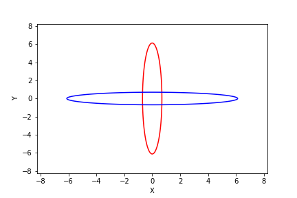
(a)

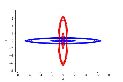
(b)

Figure 5: Shows samples of joint distributions from the same priors on parameters of the cause and effect, but with different causal models. Red shows the joint of the causal model $\textbf{\color[rgb]{0.00,0.0,1.0}X}\!\rightarrow\!Y$ and blue shows the joint of the causal model $X\!\leftarrow\!\textbf{\color[rgb]{0.00,0.0,1.0}Y}$. The contours are plotted for the same draw of parameters, showing that the different causal models will explain different joint distributions well.

D.2 Normalised linear Gaussian model

We conduct the same procedure as above, but ensure that the marginal distributions of $X$ and $Y$ are normalised to $\mathcal{N}(0,1)$. Figure 6 (a) shows the contours of one such joint distribution for the two causal models $\textbf{\color[rgb]{0.00,0.0,1.0}X}\!\rightarrow\!Y$ and $X\!\leftarrow\!\textbf{\color[rgb]{0.00,0.0,1.0}Y}$, while (b) shows 10 such joints. We can see that the joints completely overlap for the two causal models, hence the Bayesian model selection will have no opinion on the true causal model, and will convey this uncertainty.

We can show this mathematically by assuming the data samples has been generated as follows

$$\Pi(X|a_{0},\sigma_{0}) =\mathcal{N}(a_{0},\sigma_{0}^{2}),$$ (72)

$$\Pi(Y|X,a_{1},\sigma_{1}) =\mathcal{N}(a_{1}X,\sigma_{1}^{2}).$$ (73)

On normalisation, we create two new variables $X^{\prime}$ and $Y^{\prime}$ that have a standard normal distribution. Accordingly, we set $X^{\prime}=\frac{X-a_{0}}{\sigma_{0}}$ and $Y^{\prime}=\frac{Y-a_{0}a_{1}}{\sqrt{\sigma_{1}^{2}+\sigma_{0}^{2}a_{1}^{2}}}$, with distributions

$$\Pi(X^{\prime}) =\mathcal{N}(0,1),$$ (74)

$$\Pi(Y^{\prime}|X^{\prime},a_{1},\sigma_{0},\sigma_{1}) =\mathcal{N}\mathopen{}\mathclose{{}\left(\frac{\sigma_{0}a_{1}}{\sqrt{\sigma_{1}^{2}+\sigma_{0}^{2}a_{1}^{2}}}X^{\prime},\frac{\sigma_{1}^{2}}{\sigma_{1}^{2}+\sigma_{0}^{2}a_{1}^{2}}}\right).$$ (75)

We can see that both $\Pi(X^{\prime})$ and $\Pi(Y^{\prime})$ are standard normal. The anticausal factorisation in this case results in the exact same distribution. Using simple algebra we get

$$\Pi(Y^{\prime}) =\mathcal{N}(0,1),$$ (76)

$$\Pi(X^{\prime}|Y^{\prime},a_{1},\sigma_{0},\sigma_{1}) =\mathcal{N}\mathopen{}\mathclose{{}\left(\frac{\sigma_{0}a_{1}}{\sqrt{\sigma_{1}^{2}+\sigma_{0}^{2}a_{1}^{2}}}Y^{\prime},\frac{\sigma_{1}^{2}}{\sigma_{1}^{2}+\sigma_{0}^{2}a_{1}^{2}}}\right).$$ (77)

Hence, both causal factorisations imply exactly the same distribution and no prior can distinguish causal direction.

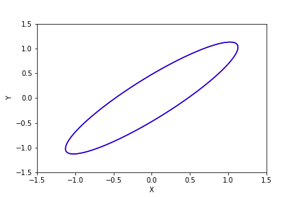
(a)

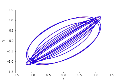
(b)

Figure 6: Best viewed in colour. Joint contours for normalised cause and effect. The joint contours completely overlap for the two causal models. Hence, both causal models will explain both datasets equally well.

D.3 Gaussian Process Latent variable model

We refer the reader to Rasmussen [44] for an introduction to Gaussian processes. We can show that for our model choice, the GPLVM, the prior results the two casual models described in section 4.1 having different dataset densities. We consider the model $\mathcal{M}_{\textbf{\color[rgb]{0.00,0.0,1.0}X}\!\rightarrow\!Y}$ in this section, but we leave out the notation $\mathcal{M}_{\textbf{\color[rgb]{0.00,0.0,1.0}X}\!\rightarrow\!Y}$ for clarity. Note that the final dataset density is found by integrating over the hyperparameters as laid out in app. B, for clarity, we leave that step out of this section. In $\mathcal{M}_{\textbf{\color[rgb]{0.00,0.0,1.0}X}\!\rightarrow\!Y}$, $\mathbf{x}$ is modelled by itself and $\mathbf{y}$ is modelled conditioned on $\mathbf{x}$. For the estimation of $\mathbf{x}$ we have

$$p(\mathbf{x},\mathbf{f}_{X},\mathbf{w}_{X}|\lambda_{X})=p(\mathbf{x}|\mathbf{f}_{X})p(\mathbf{f}_{X}|\mathbf{w}_{X},\lambda_{X})p(\mathbf{w}_{X}),$$ (78)

where $\lambda_{X}$ collects all the hyperparameters for modelling $\mathbf{x}$. The dataset density can be found by integrating over the priors

$$p(\mathbf{x}|\lambda_{X}) =\iint p(\mathbf{x}|\mathbf{f}_{X})p(\mathbf{f}_{X}|\mathbf{w}_{X},\lambda_{X})p(\mathbf{w}_{X})d\mathbf{f}_{X}d\mathbf{w}_{X}$$ (79)

$$=\int p(\mathbf{x}|\mathbf{w}_{X},\lambda_{X})p(\mathbf{w}_{X})d\mathbf{w}_{X},$$ (80)

where $p(\mathbf{x}|\mathbf{w}_{X},\lambda_{X})=\mathcal{N}(0,K_{\lambda_{X}}(\mathbf{w}_{X},\mathbf{w}_{X}^{\prime})+\sigma^{2}_{X})$, $\sigma^{2}_{X}$ is the likelihood noise hyperparameter and $K_{\lambda_{X}}$ is the chosen kernel with hyperparameters $\lambda_{X}$. All modelling choices are those laid out in section 5. $p(\mathbf{w}_{X})$ is usually chosen to be standard Gaussian distribution. From this, we can see that the dataset density is a mixture of Gaussians mixed by Gaussian distributed weights. Similarly, for the conditional model $\mathbf{y}|\mathbf{x}$ we have

$$p(\mathbf{y}|\mathbf{x},\lambda_{Y}) =\iint p(\mathbf{y}|\mathbf{x},\mathbf{f}_{Y})p(\mathbf{f}_{Y}|\mathbf{w}_{Y},\lambda_{Y})p(\mathbf{w}_{Y})d\mathbf{f}_{Y}d\mathbf{w}_{Y}$$ (81)

$$=\int p(\mathbf{y}|\mathbf{x},\mathbf{w}_{Y},\lambda_{Y})p(\mathbf{w}_{Y})d\mathbf{w}_{Y},$$ (82)

where $p(\mathbf{y}|\mathbf{x},\mathbf{w}_{Y},\lambda_{Y})=\mathcal{N}(0,K_{\lambda_{Y}}((\mathbf{x},\mathbf{w}_{Y}),(\mathbf{x},\mathbf{w}_{Y})^{\prime})+\sigma^{2}_{Y})$, and $p(\mathbf{w}_{Y})$ is a standard Gaussian.

Using Bayes rule, we can find the implied dataset densities of the anticausal factorisation of $\mathcal{M}_{\textbf{\color[rgb]{0.00,0.0,1.0}X}\!\rightarrow\!Y}$. We show that this will have a very different form to the causal factorisation for the causal model $\mathcal{M}_{X\!\leftarrow\!\textbf{\color[rgb]{0.00,0.0,1.0}Y}}$, hence the two causal models will imply different dataset densities. For the marginal on $\mathbf{y}$ we can integrate over $\mathbf{f}_{X}$ and $\mathbf{f}_{Y}$

$$p(\mathbf{y}|\mathbf{w}_{X},\mathbf{w}_{Y},\lambda_{X},\lambda_{Y})=\int p(\mathbf{x}|\mathbf{w}_{X},\lambda_{X})p(\mathbf{y}|\mathbf{x},\mathbf{w}_{Y},\lambda_{Y})d\mathbf{x},$$

with

$$p(\mathbf{x}|\mathbf{w}_{X},\lambda_{X}) =\mathcal{N}(0,K_{\lambda_{X}}(\mathbf{w}_{X},\mathbf{w}_{X}^{\prime})+\sigma^{2}_{X}),$$ (83)

$$p(\mathbf{y}|\mathbf{x},\mathbf{w}_{Y},\lambda_{Y}) =\mathcal{N}(0,K_{\lambda_{Y}}((\mathbf{x},\mathbf{w}_{Y}),(\mathbf{x},\mathbf{w}_{Y})^{\prime})+\sigma^{2}_{Y}).$$ (84)

As $K$ is a complicated non-linear function in general, we can see that after integrating over $\mathbf{x}$, $p(\mathbf{y}|\mathbf{w}_{X},\mathbf{w}_{Y},\lambda_{X},\lambda_{Y})$ will not be a Gaussian distribution. Hence, the dataset density $p(\mathbf{y}|\lambda_{X},\lambda_{Y})$ will not be a mixture of Gaussians, but a more complicated mixture. Furthermore, whereas to estimate the dataset density of $\mathbf{x}$, we only had to integrate over one function $\mathbf{f}$ and latent $\mathbf{w}$, the anticausal factorisation requires integrating over both functions and latents. Hence, the marginal dataset density of $\mathbf{y}$ estimated by $\mathcal{M}_{X\!\leftarrow\!\textbf{\color[rgb]{0.00,0.0,1.0}Y}}$ will in general not be equal to the marginal density of $\mathbf{y}$ implied by the anticausal factorisation of $\mathcal{M}_{\textbf{\color[rgb]{0.00,0.0,1.0}X}\!\rightarrow\!Y}$. A similar argument holds for the implied anticausal conditional $p(\mathbf{x}|\mathbf{y},\lambda_{X},\lambda_{Y})$. This shows that the choices of priors in GPLVM will not imply the same dataset density in both causal models. We have shown this by showing that though the causal factorisation of a model follows the form of a GPLVM prior, the anticausal factorisation does not.

Appendix E Additional Experiments

We carry out some additional experiments that give us insight into our method. In section E.1, we show that importance of modelling the joint instead of just the conditional or marginal densities.

E.1 Only modelling the conditional or marginal

Methods such that ANM, PNL, SLOPPY, RECI only model the conditional densities to find the causal direction. In fact, methods such as SLOPPY base their theory on modelling the joint, but make the assumption that the cause is always Gaussian distributed, and hence only consider the conditional. The Kolmogorov complexity formalisation of the ICM principle [27, 42] also considers the whole joint.

We show that modelling the joint is crucial to our approach, and that we suffer a degradation in performance when only considering one component - the marginal or conditional. In table 3, we show that results of the same model, but making the decision on the predicted causal model with the joint, the conditional, or with the marginal. The results corroborate with our theory.

Table 3: Results of making the decision on the predicted causal model with the full joint, or just with the marginal or conditional densities. In accordance with our theory, modelling the joint is important. The numbers are ROCAUC (higher is better).

Methods	CE-Cha	CE-Multi	CE-Net	CE-Gauss	CE-Tueb
GPLVM - Joint	81.9	97.7	98.9	89.3	78.3
GPLVM - Conditional	61.5	89.7	70.3	21.7	36.2
GPLVM - Marginal	44.5	23.3	42.6	83.1	75.7

Appendix F Derivations for section 4.3

F.1 Derivation of the probability of error of both models being the same

Here we show that the probability of error of both the models is exactly the same. The dataset densities of the two models are

$$p(\mathbf{x},\mathbf{y}|\mathcal{M}_{\textbf{\color[rgb]{0.00,0.0,1.0}X}\!\rightarrow\!Y}) =\int p(\mathbf{x}|\phi,\mathcal{M}_{\textbf{\color[rgb]{0.00,0.0,1.0}X}\!\rightarrow\!Y})p(\phi|\mathcal{M}_{\textbf{\color[rgb]{0.00,0.0,1.0}X}\!\rightarrow\!Y})\mathrm{d}\phi\int p(\mathbf{y}|\mathbf{x},\theta,\mathcal{M}_{\textbf{\color[rgb]{0.00,0.0,1.0}X}\!\rightarrow\!Y})p(\theta|\mathcal{M}_{\textbf{\color[rgb]{0.00,0.0,1.0}X}\!\rightarrow\!Y})\mathrm{d}\theta\,,$$ (85)

$$p(\mathbf{x},\mathbf{y}|\mathcal{M}_{X\!\leftarrow\!\textbf{\color[rgb]{0.00,0.0,1.0}Y}}) =\int p(\mathbf{y}|\phi,\mathcal{M}_{X\!\leftarrow\!\textbf{\color[rgb]{0.00,0.0,1.0}Y}})p(\phi|\mathcal{M}_{X\!\leftarrow\!\textbf{\color[rgb]{0.00,0.0,1.0}Y}})\mathrm{d}\phi\int p(\mathbf{x}|\mathbf{y},\theta,\mathcal{M}_{X\!\leftarrow\!\textbf{\color[rgb]{0.00,0.0,1.0}Y}})p(\theta|\mathcal{M}_{X\!\leftarrow\!\textbf{\color[rgb]{0.00,0.0,1.0}Y}})\mathrm{d}\theta\,.$$ (86)

The marginal and conditional densities in the above are chosen from the same families, and $p(\phi|\mathcal{M}_{\textbf{\color[rgb]{0.00,0.0,1.0}X}\!\rightarrow\!Y})=p(\phi|\mathcal{M}_{X\!\leftarrow\!\textbf{\color[rgb]{0.00,0.0,1.0}Y}})$ as well as $p(\theta|\mathcal{M}_{\textbf{\color[rgb]{0.00,0.0,1.0}X}\!\rightarrow\!Y})=p(\theta|\mathcal{M}_{X\!\leftarrow\!\textbf{\color[rgb]{0.00,0.0,1.0}Y}})$. Thus, $p(\mathbf{x},\mathbf{y}|\mathcal{M}_{\textbf{\color[rgb]{0.00,0.0,1.0}X}\!\rightarrow\!Y})=p(\mathbf{y},\mathbf{x}|\mathcal{M}_{X\!\leftarrow\!\textbf{\color[rgb]{0.00,0.0,1.0}Y}})$. That is, swapping $\mathbf{x}$ and $\mathbf{y}$ in one model will give the dataset density of the other model. We can use this to show

$$P(E|\mathcal{M}_{\textbf{\color[rgb]{0.00,0.0,1.0}X}\!\rightarrow\!Y}) =\int_{\mathcal{R}}p(\mathbf{x},\mathbf{y}|\mathcal{M}_{\textbf{\color[rgb]{0.00,0.0,1.0}X}\!\rightarrow\!Y})\mathrm{d}(\mathbf{x},\mathbf{y})\,, \mathcal{R}=\{(\mathbf{x},\mathbf{y})\,\,|\,\,p(\mathbf{x},\mathbf{y}|\mathcal{M}_{X\!\leftarrow\!\textbf{\color[rgb]{0.00,0.0,1.0}Y}})>p(\mathbf{x},\mathbf{y}|\mathcal{M}_{\textbf{\color[rgb]{0.00,0.0,1.0}X}\!\rightarrow\!Y})\}$$ (87)

$$=\int_{\mathcal{R}}p(\mathbf{y},\mathbf{x}|\mathcal{M}_{X\!\leftarrow\!\textbf{\color[rgb]{0.00,0.0,1.0}Y}})\mathrm{d}(\mathbf{x},\mathbf{y})\,, \mathcal{R}=\{(\mathbf{x},\mathbf{y})\,\,|\,\,p(\mathbf{y},\mathbf{x}|\mathcal{M}_{\textbf{\color[rgb]{0.00,0.0,1.0}X}\!\rightarrow\!Y})>p(\mathbf{y},\mathbf{x}|\mathcal{M}_{X\!\leftarrow\!\textbf{\color[rgb]{0.00,0.0,1.0}Y}})\}$$ (88)

$$=P(E|\mathcal{M}_{X\!\leftarrow\!\textbf{\color[rgb]{0.00,0.0,1.0}Y}}).$$ (89)

F.2 Upper bound on standard deviation of probability of error

The probability of error is

$$P(\text{Error}) =P(\text{Error}|\mathcal{M}_{\textbf{\color[rgb]{0.00,0.0,1.0}X}\!\rightarrow\!Y})$$ (90)

$$=\int\mathbb{I}[\mathcal{D}\in\mathcal{R}]\cdot p(\mathcal{D}|\mathcal{M}_{\textbf{\color[rgb]{0.00,0.0,1.0}X}\!\rightarrow\!Y})\mathrm{d}\mathcal{D}$$ (91)

$$\hat{I} =\frac{1}{T}\sum_{t=1}^{T}\mathbb{I}[\mathcal{D}_{t}\in\mathcal{R}],\ \ \mathcal{D}_{t}\sim p(\mathcal{D}|\mathcal{M}_{\textbf{\color[rgb]{0.00,0.0,1.0}X}\!\rightarrow\!Y}),$$ (92)

where $\mathbb{I}[\cdot]$ is the indicator function and $\hat{I}$ is the Monte Carlo estimator of $P(\text{Error})$. We can bound the variance by using the fact that $\text{Var}(\mathbb{I}[\mathcal{D}_{t}\in\mathcal{R}])\leq 0.25$ if we treat $\mathbb{I}[\cdot]$ as a Bernoulli distributed random variable. We now get

$$\text{Var}(\hat{I}) \leq\frac{1}{4T}.$$ (93)

This can be calculated numerically.

Appendix G Model Details

Here, we provide a more in depth introduction to our model and approximations.

G.1 Latent variable Gaussian Processes with inducing points

Gaussian processes (GPs) [44] are non-parametric Bayesian models that define a prior over functions. The form of the prior is controlled by choice of a kernel function, $\mathbf{K}$. Specifically, the kernel defines a covariance over outputs for the function. The kernels are parametrised by continuous hyperparameters. Adding kernels together and varying their hyperparameters allows for constructing flexible priors that cover a wide range of functions.

Latent variable Gaussian Processes (GPLVM) consider a latent noise term $\mathbf{w}$ as an input with an associated prior. Integrating over the noise term allows for modelling heteroscedastic noise as well as non Gaussian likelihoods. GPs have a well known cost of $\mathcal{O}(N^{3})$ where $N$ is the number of samples, this prohibits their application to large datasets. To allow for scalability, we use the inducing points approximation [54, 23]. Here, we approximate the inputs $\mathbf{x}$ and latents $\mathbf{w}$ with $M<N$ inducing inputs $\mathbf{z}$, and their corresponding outputs with $\mathbf{u}$. This formulation now has a cost of $\mathcal{O}(M^{3})$.

We collectively denote all hyperparameters of the model with $\bm{\lambda}$. The latent variable Gaussian process for modelling $p(\mathbf{y}|\mathbf{x},\bm{\lambda})$ has the following form

$$\mathbf{y}|\mathbf{x},\mathbf{w}\sim\mathcal{N}(\mathbf{f}(\mathbf{x},\mathbf{w}),\sigma^{2}),\ \ \ \ \mathbf{F}|\mathbf{u}\sim\mathcal{N}(\mathbf{K}_{\mathbf{fu}}\mathbf{K}_{\mathbf{uu}}^{-1}\mathbf{u},\mathbf{\Sigma}),$$

$$\mathbf{u}\sim\mathcal{N}(\mathbf{0},\mathbf{K}_{\mathbf{uu}}),\ \ \ \ \ \ \ \ \ \ \ \ \ \ \ \ \ \ \ [\mathbf{K}_{\mathbf{ff}}]_{nn^{\prime}}=\mathbf{K}(x_{n},x_{n^{\prime}}),$$

where $\Sigma=\mathbf{K}_{\mathbf{ff}}-\mathbf{K}_{\mathbf{fu}}\mathbf{K}_{\mathbf{uu}}^{-1}\mathbf{K}_{\mathbf{uf}}$, and $\sigma$ denotes the likelihood noise hyperparameter. We posit an approximate posterior over the latents $q(\mathbf{w})$ and inducing outputs $q(\mathbf{u})$ following the variational inference framework. This gives a lower bound to the log marginal likelihood that can be maximised with respect to the variational distributions $q$ and the inducing inputs $\mathbf{z}$. The lower bound for the conditional $p(\mathbf{y}|\mathbf{x},\bm{\lambda})$ has the form

$$\mathcal{L}_{\mathbf{y}|\mathbf{x}}(q,\mathbf{z},\bm{\lambda})\!\!:=\!\!\sum_{n}\mathbb{E}_{q(w_{n})q(\mathbf{u})p(\mathbf{f}|\mathbf{u})}\mathopen{}\mathclose{{}\left[\log p(y_{n}|x_{n},w_{n})}\right]\!+\!KL[q(\mathbf{w})||p(\mathbf{w})]\!+\!KL[q(\mathbf{u})||p(\mathbf{u})].$$ (94)

For smaller datasets, we follow the steps in Titsias and Lawrence [55] and analytically integrate over $p(\mathbf{f}|\mathbf{u})$ first and then find the closed form solution for $q(\mathbf{u})$ — denoted GPLVM-closed form. For certain kernels, for example the RBF and linear kernels, we can analytically find the expectation under $q(w_{n})$ of the remaining first term in eq. 94. For larger datasets, we need to use stochastic variational inference [23] as finding the closed form solutions are prohibitive — we denote this GPLVM-stochastic. This requires using doubly stochastic variational inference to calculate the expectations [32]. We assume a standard Gaussian distribution for $p(\mathbf{w})$ and a Gaussian for $q(\mathbf{w})$ with variational parameters that are to be trained. The final KL term is between two Gaussians and is analytically tractable. We use the evidence approximation for the hyperparameters, which we detail in app. B.

The bound for all the marginal and conditional models, $p(\mathbf{y}|\mathbf{x})$, $p(\mathbf{x})$, $p(\mathbf{x}|\mathbf{y})$, and $p(\mathbf{y})$, follows the form of eq. 94. We assume the same kernels and priors for all the models as well.

G.2 Final Score

To model each distribution, we maximise the lower bound with respect to the variational distributions $q$ and inducing inputs $\mathbf{z}$ to tighten the bound. Simultaneously, we maximise the lower bound with respect to the kernel hyperparameters and the likelihood noise, collectively denoted as $\bm{\lambda}$. The final scores we calculate are

$$\mathcal{F}_{X\rightarrow Y} =\mathcal{L}_{\mathbf{x}}(\hat{q},\hat{\mathbf{z}},\hat{\bm{\lambda}})+\mathcal{L}_{\mathbf{y}|\mathbf{x}}(\hat{q},\hat{\mathbf{z}},\hat{\bm{\lambda}}),$$ (95)

$$\mathcal{F}_{Y\rightarrow X} =\mathcal{L}_{\mathbf{y}}(\hat{q},\hat{\mathbf{z}},\hat{\bm{\lambda}})+\mathcal{L}_{\mathbf{x}|\mathbf{y}}(\hat{q},\hat{\mathbf{z}},\hat{\bm{\lambda}}),$$ (96)

where $(\hat{q},\hat{\mathbf{z}},\hat{\bm{\lambda}})$ denote the values the maximise the corresponding lower bound. We finally infer the predicted causal model as $\mathcal{M}_{X\rightarrow Y}$ if $\mathcal{F}_{X\rightarrow Y}>\mathcal{F}_{Y\rightarrow X}$, $\mathcal{M}_{Y\rightarrow X}$ if $\mathcal{F}_{Y\rightarrow X}>\mathcal{F}_{X\rightarrow Y}$, and undecided otherwise.

Appendix H Experiment Details

We outline the experimental details of our method. As we implement SLOPPY, we also outline the details of the settings we used. The results for the rest of the baselines were taken from [19] and [8].

H.1 Dataset details

CE-Cha: A mixture of synthetic and real world data. Taken from the cause-effect pairs challenge [19].

CE-Multi [15]: Synthetic data with effects generated with varying noise relationships. The noise relationships are pre-additive $(f(X+E))$, post-additive $(f(X)+E)$, pre-multiplicative $(f(X\times E))$, or post-multiplicative $(f(X)\times E)$. The function is linear or polynomial.

CE-Net [15]: Synthetic data with randomly initialised neural networks for functions and random exponential family distributions chosen for the cause.

CE-Gauss [39]: Synthetic data generated with random noise distributions $E_{1},E_{2}$ defined in [39]. The cause and effect are generated according to $X=f_{x}(E_{1})$ and $Y=f_{y}(X,E_{2})$, where $f_{x},f_{y}$ are sampled from Gaussian processes.

CE-Tueb [39]: Contains 105 pairs of real cause effect pairs taken from the UCI dataset. We use the version dating August 22, 2016. We also remove high dimensional datasets leaving 99 datasets in total.

H.2 GPLVM details

For GPLVM-closed form, we use the sum of an RBF and linear kernels. $q(w_{n})$ has an analytical expectation for these kernels, as discussed in section G.1. As detailed in section G.1, we find the optimal form of $q(\bm{u})$ following the procedure of [55]. We use 200 inducing points for all experiments. The model was first trained using Adam with a learning rate of 0.1. After 20,000 epochs, the model was trained using BFGS. We found that this greatly helped the numerical instability of BFGS, but found better ELBO (variational approximation to the marginal likelihood) values than simply using Adam.

For GPLVM-stochastic, as expectations are calculated by sampling, it was possible to use a larger number of kernels. We used a sum of RBF, Linear, Matern32 and Rational Quadratic kernels. 10 samples were used to calculate the expectations. The model was trained with Adam with a learning rate of 0.05. The model stopped training if the value of the ELBO plateaued, else it ran for a maximum of 100,000 epochs. In our experiments, we only use GPLVM-stochastic for CE-Tueb as it had a few datasets that had a large number of samples.

The approximate posteriors for both the models $q(w_{n})$ are initialised with low variance and the mean equal to $0.01$ times the output. This reduced the instability during optimisation.

As GPLVMs are known to suffer from local optima issues, we use 20 random restarts of hyperparameter initialisations and choose the highest estimate of the approximate marginal likelihood as the final score. For the various hyperparameters, the sampling procedures were:

1. The kernel variances were always set to 1.

2. The likelihood variances were sampled by first sampling $\kappa\sim\text{Uniform}(10,100)$, and then $\sigma^{2}_{\text{Likelihood}}=1/\kappa^{2}$.

3. The kernel lengthscales were sampled by first sampling $\psi\sim\text{Uniform}(1,100)$, then set $\lambda_{\text{Lengthscale}}=1/\psi$.

H.3 SLOPPY details

For benchmarking the SLOPPY method, we use the author’s code [36]. We use the spline estimator as it performs better on all the dataset. For this estimator, we select the best performing regularisation metric between the AIC and BIC.

References

- Bernardo and Smith [2009] José M Bernardo and Adrian FM Smith. Bayesian theory, volume 405. John Wiley & Sons, 2009.
- Blei et al. [2017] David M Blei, Alp Kucukelbir, and Jon D McAuliffe. Variational inference: A review for statisticians. Journal of the American statistical Association, 112(518), 2017.
- Blöbaum et al. [2018] Patrick Blöbaum, Dominik Janzing, Takashi Washio, Shohei Shimizu, and Bernhard Schölkopf. Cause-effect inference by comparing regression errors. In International Conference on Artificial Intelligence and Statistics, 2018.
- Bühlmann [2020] Peter Bühlmann. Invariance, causality and robustness. Statistical Science, 35(3), 2020.
- Chickering [2002] David Maxwell Chickering. Optimal structure identification with greedy search. Journal of machine learning research, 3(Nov), 2002.
- Damianou and Lawrence [2013] Andreas Damianou and Neil D Lawrence. Deep gaussian processes. In Artificial intelligence and statistics. PMLR, 2013.
- Daniusis et al. [2012] Povilas Daniusis, Dominik Janzing, Joris Mooij, Jakob Zscheischler, Bastian Steudel, Kun Zhang, and Bernhard Schölkopf. Inferring deterministic causal relations. arXiv preprint arXiv:1203.3475, 2012.
- Duong and Nguyen [2021] Bao Duong and Thin Nguyen. Bivariate causal discovery via conditional divergence. In First Conference on Causal Learning and Reasoning, 2021.
- Dutordoir et al. [2018] Vincent Dutordoir, Hugh Salimbeni, James Hensman, and Marc Deisenroth. Gaussian process conditional density estimation. Advances in neural information processing systems, 31, 2018.
- Fonollosa [2019] José AR Fonollosa. Conditional distribution variability measures for causality detection. In Cause Effect Pairs in Machine Learning. Springer, 2019.
- Friedman and Nachman [2000] Nir Friedman and Iftach Nachman. Gaussian process networks. In Proceedings of the Sixteenth conference on Uncertainty in artificial intelligence, 2000.
- Geiger and Heckerman [2002] Dan Geiger and David Heckerman. Parameter priors for directed acyclic graphical models and the characterization of several probability distributions. The Annals of Statistics, 30(5), 2002.
- Gelman et al. [2013] Andrew Gelman, John B Carlin, Hal S Stern, David B Dunson, Aki Vehtari, and Donald B Rubin. Bayesian data analysis. CRC press, 2013.
- [14] Jayanta K Ghosh, Mohan Delampady, and Tapas Samanta. An introduction to Bayesian analysis: theory and methods, volume 725. Springer.
- Goudet et al. [2018] Olivier Goudet, Diviyan Kalainathan, Philippe Caillou, Isabelle Guyon, David Lopez-Paz, and Michele Sebag. Learning functional causal models with generative neural networks. In Explainable and interpretable models in computer vision and machine learning. Springer, 2018.
- Grunwald and Vitányi [2004] Peter Grunwald and Paul Vitányi. Shannon information and kolmogorov complexity. arXiv preprint cs/0410002, 2004.
- Grünwald [2007] Peter D Grünwald. The minimum description length principle. MIT press, 2007.
- Guo et al. [2022] Siyuan Guo, Viktor Tóth, Bernhard Schölkopf, and Ferenc Huszár. Causal de finetti: On the identification of invariant causal structure in exchangeable data. arXiv preprint arXiv:2203.15756, 2022.
- Guyon et al. [2019] Isabelle Guyon, Olivier Goudet, and Diviyan Kalainathan. Evaluation methods of cause-effect pairs. In Cause Effect Pairs in Machine Learning, chapter 2. Springer, 2019.
- Heckerman [1995] David Heckerman. A bayesian approach to learning causal networks. In Proceedings of the Eleventh conference on Uncertainty in artificial intelligence, pages 285–295, 1995.
- Heckerman et al. [1995] David Heckerman, Dan Geiger, and David M Chickering. Learning bayesian networks: The combination of knowledge and statistical data. Machine learning, 20(3), 1995.
- Heckerman et al. [2006] David Heckerman, Christopher Meek, and Gregory Cooper. A bayesian approach to causal discovery. Innovations in Machine Learning: Theory and Applications, 2006.
- Hensman et al. [2013] James Hensman, Nicolo Fusi, and Neil D Lawrence. Gaussian processes for big data. arXiv preprint arXiv:1309.6835, 2013.
- Hewitt and Savage [1955] Edwin Hewitt and Leonard J Savage. Symmetric measures on cartesian products. Transactions of the American Mathematical Society, 80(2), 1955.
- Hoyer et al. [2008] Patrik Hoyer, Dominik Janzing, Joris M Mooij, Jonas Peters, and Bernhard Schölkopf. Nonlinear causal discovery with additive noise models. Advances in neural information processing systems, 21, 2008.
- Immer et al. [2022] Alexander Immer, Christoph Schultheiss, Julia E Vogt, Bernhard Schölkopf, Peter Bühlmann, and Alexander Marx. On the identifiability and estimation of causal location-scale noise models. arXiv preprint arXiv:2210.09054, 2022.