Exploring the linear space of Feynman integrals via generating functions

Abstract

Deriving a comprehensive set of reduction rules for Feynman integrals has been a longstanding challenge. In this paper, we present a proposed solution to this problem utilizing generating functions of Feynman integrals. By establishing and solving differential equations of these generating functions, we are able to derive a system of reduction rules that effectively reduce any associated Feynman integrals to their bases. We illustrate this method through various examples and observe its potential value in numerous scenarios.

I Introduction

Scattering amplitudes play a crucial role in quantum field theory as they connect theoretical predictions with experimental observations. With the successful operation of the Large Hadron Collider [1, 2] and the proposal of next-generation colliders[3, 4, 5, 6, 7, 8, 9, 10], perturbative calculations of scattering processes need to be pushed to higher orders, such as next-to-next-to-leading order, to match the precision of experimental measurements. This requirement necessitates the computation of scattering amplitudes at multiloop levels. Utilizing Lorentz symmetry, these amplitudes can be expressed as linear combinations of scalar Feynman integrals (FIs). The calculation of scalar FIs poses a significant challenge for state-of-the-art problems.

A family of scalar FIs can be represented as

$$I(\vec{\nu})=\int\prod_{i=1}^{L}\frac{\mathrm{d}^{D}\ell_{i}}{\mathrm{i}\pi^{D/2}}\frac{\mathcal{D}_{K+1}^{-\nu_{K+1}}\cdots\mathcal{D}_{N}^{-\nu_{N}}}{\mathcal{D}_{1}^{\nu_{1}}\cdots\mathcal{D}_{K}^{\nu_{K}}},$$ (1)

where $D=4-2\epsilon$ represents the spacetime dimension, $L$ is the number of loops, $\ell_{i}$ are the loop momenta, $\mathcal{D}_{1},\ldots,\mathcal{D}_{K}$ are the inverse propagators, $\mathcal{D}_{K+1},\ldots,\mathcal{D}_{N}$ are the irreducible scalar products (ISPs) introduced for completeness, $\nu_{1},\ldots,\nu_{K}$ can be any integers, and $\nu_{K+1},\ldots,\nu_{N}$ can only be non-positive integers. The rank of an integral is defined as the opposite value of the sum of all negative powers, and the dots of an integral represent the sum of all positive powers subtracted by the number of positive indices. For instance, the integral $I(1,2,2,3,-1,-2)$ has rank 3 and dots 4.

It has been proven that a family of FIs forms a finite-dimensional linear space [11] with bases known as master integrals (MIs). Therefore, the prevailing method for calculating scalar FIs involves two distinct tasks. The first task is FIs reduction, which aims to express FIs as linear combinations of MIs [12, 13, 14, 15, 16, 17, 18, 19, 20, 21, 22, 23, 24, 25, 26, 27, 28, 29, 30, 31, 32, 33, 34, 35, 36, 37, 38, 39, 40, 41, 42, 43, 44, 45, 46, 47, 48, 49, 50, 51, 52]; While the second is to compute these MIs [53, 54, 55, 56, 57, 58, 59, 60, 61, 62, 63, 64, 65, 66, 67, 68, 69, 70, 71, 72, 73, 74, 75, 76, 77, 78, 79, 80, 81, 13, 82, 83, 84, 85, 86, 87, 88, 89, 90, 91, 92, 93, 94, 95, 96, 97, 98, 99, 100, 101, 102, 103, 104, 105, 106, 107]. Notably, based on the auxiliary mass flow method [100, 101, 102, 103, 104, 105], any given FI can be automatically calculated to high precision as far as the reduction has been achieved. However, FIs reduction is a critical yet formidable task in complicated multiloop processes.

Integration-by-parts (IBP) identities [12] combining with the Laporta algorithm [14] is a widely-used approach to realize reduction. Even though powered by the finite field method [21, 22, 23, 24, 25, 26] to avoid intermediate expression swell, and syzygy equations[17, 18, 108, 19, 109, 110, 111, 112, 113, 114] and block-triangular form [27, 28, 29] to reduce the size of IBP system, reduction of FIs with high power of denominators or ISPs is still extremely time- and resource-consuming. Various other methods have been proposed to bypass IBP, but each approach has its own difficulties. For instance, in the method based on intersection theory [44, 45, 46, 47], the calculation of intersection numbers for multi-variable problems remains challenging; In the methods based on large spacetime expansion [15, 16] or large auxiliary mass expansion [27], it is hard to obtain very higher order expansion terms.

For a long time, the ultimate goal of FIs reduction has been to find a complete set of reduction rules, known as recurrence relations, with general powers $\vec{\nu}$. These recurrence relations should efficiently reduce all integrals in a family to the MIs. For simple problems, such recurrence relations can be constructed by analyzing IBP identities manually, see e.g Refs. [12, 115, 116, 117, 118, 119, 120] for early works. There are also very powerful reduction programs for specific problems, which can tackle massive tadpoles, like MATAD [121], massless self-energy topoly at three and four loop, respectively, called MINCER [122, 123] and FORCER [124]. A tailored heuristical approach for general problems is also available in LiteRed [41]. However, these construction procedures are obscure and success is not guaranteed.

From an algebraic geometry perspective, the establishment of recurrence relations becomes possible once the Gröbner bases are known. Gröbner bases serve as a fundamental tool in the analysis of polynomial ideals, and significant efforts have been dedicated to this area of research [125, 126, 127, 128, 129, 130, 131]. However, computing Gröbner bases for the noncommutative algebra generated by the IBP relations remains an exceedingly challenging task.

In this paper, we propose a general approach to deriving recurrence relations for arbitrary Feynman integral families by setting up and solving differential equations (DEs) for generating functions (GFs) associated with these integrals. By doing so, we are able to effectively reduce the infinite number of Feynman integrals within a family to a finite set of MIs. This reduction is achieved through solving a linear system with finite size, thereby providing a solution to this long-standing and challenging problem with reasonable computational complexity.

We employ the recently released Blade package [29] to construct DEs of GFs. To demonstrate the performance of the GF method, we apply it to some examples, spanning from simple and straightforward problems to cutting-edge and complex scenarios.

II Generating functions

Our approach is motivated by the auxiliary mass flow method [27], where by introducing an auxiliary mass term $\eta$ to each denominator and expanding around $\eta=0$ using DEs w.r.t. $\eta$, one can obtain values of a series of FIs with arbitrary powers of denominators. It means that the FI with auxiliary masses serves as a GF of these original FIs. Similar ideas have also been presented in Ref. [125], where Gröbner bases are computed by solving DEs when all propagators, including ISPs, have different masses. In Ref. [132], the summation of the non-standard term $(\Delta\cdot p)^{n}$ into a linear propagator $1/(1-x\Delta\cdot p)$ constructs a kind of GF and has been used in[133, 134, 135] for reduction of high rank integrals. In Refs. [136], GFs are employed to reduce arbitrary one-loop tensor integrals by introducing an auxiliary vector [137, 138, 139, 140, 141]. In this paper, we propose to use GF method to reduce all FIs in any given family.

One choice of GFs for the integral family in Eq. (1) can be defined as follows:

$$\begin{split}G_{\vec{\nu}}(\vec{x},\vec{\eta})&=\int\prod_{i=1}^{L}\frac{\mathrm{d}^{D}\ell_{i}}{\mathrm{i}\pi^{D/2}}\frac{e^{Z^{\vec{x}}}\prod_{i=K+1}^{N}{\cal D}_{i}^{-\nu_{i}}}{\prod_{i=1}^{K}({\cal D}_{i}-\eta_{i})^{\nu_{i}}},\end{split}$$ (2)

with top-sector corner integral given by

$$\begin{split}G_{{\text{top}}}(\vec{x},\vec{\eta})&=\int\prod_{i=1}^{L}\frac{\mathrm{d}^{D}\ell_{i}}{\mathrm{i}\pi^{D/2}}\frac{e^{Z^{\vec{x}}}}{\prod_{i=1}^{K}({\cal D}_{i}-\eta_{i})},\end{split}$$ (3)

where ${\nu}_{i}$ are given integers, $\eta_{i}$ are auxiliary masses and $Z^{\vec{x}}={\sum_{i=K+1}^{N}x_{i}{\cal D}_{i}}$ is a linear combination of ISPs. FIs in Eq. (1) can be generated from $G_{{\text{top}}}(\vec{x},\vec{\eta})$ by expanding $\eta_{i}$ around $0$ or $\infty$ and $x_{i}$ around $0$. For example, FIs in the top-sector can be generated by taking the following limit:

$$I(\vec{\nu})=\lim_{\vec{x}\rightarrow 0}\lim_{\vec{\eta}\rightarrow 0}\partial^{\vec{\nu}}_{x}\partial^{\vec{\nu}}_{\eta}G_{{\text{top}}}(\vec{x},\vec{\eta})$$ (4)

where

$$\partial^{\vec{\nu}}_{x} \equiv\prod_{i=K+1}^{N}\frac{\partial^{\nu_{i}}}{{\partial x_{i}}^{\nu_{i}}},$$ (5)

$$\partial^{\vec{\nu}}_{\eta} \equiv\prod_{i=1}^{K}\frac{1}{{(\nu_{i}-1)}!}\frac{\partial^{\nu_{i}-1}}{{\partial\eta_{i}}^{\nu_{i}-1}}.$$ (6)

Similar to FIs, using methods such as IBP method, we find that the GFs defined in Eq. (2) form a finite-dimensional linear space. We can choose a set of MIs of GFs that cover $G_{{\text{top}}}(\vec{x},\vec{\eta})$, denoted as $\vec{\cal G}(\vec{x},\vec{\eta})$, and derive DEs for them:

$$\frac{\partial}{\partial x_{i}}\vec{\cal G}= A_{i}\vec{\cal G},$$ (7)

$$\frac{\partial}{\partial\eta_{i}}\vec{\cal G}= B_{i}\vec{\cal G}.$$ (8)

Since the FIs are expansion coefficients of GFs, by expanding $\vec{\cal G}(\vec{x},\vec{\eta})$ using DEs, we can obtain a system of linear relations between FIs. These relations are the desired recurrence relations that efficiently reduce all target FIs to the minimal set of MIs. Therefore, once we obtain the DEs for the MIs of GFs, the reduction of FIs in the corresponding family is solved.

In physical Feynman amplitudes, one often encounters FIs with high rank but very small dots. In such cases, we can define simpler GFs as follows:

$$\begin{split}G_{\vec{\nu}}(\vec{x})&=\int\prod_{i=1}^{L}\frac{\mathrm{d}^{D}\ell_{i}}{\mathrm{i}\pi^{D/2}}\frac{e^{Z^{\vec{x}}}}{\prod_{i=1}^{N}{\cal D}_{i}^{\nu_{i}}},\end{split}$$ (9)

and corresponding simpler MIs $\vec{\cal G}(\vec{x})$, which have fewer extra variables. By setting up and solving partial DEs of $\vec{\cal G}(\vec{x})$ w.r.t. $x_{i}$, we can achieve the reduction of original FIs with arbitrary rank.

However, in practice, we find that there is an even better approach, denoted as fixed direction scheme, by setting

$$\vec{x}=x\vec{c},$$ (10)

where $x$ is a variable and $\vec{c}$ are some fixed numbers. With each chosen set of values for $\vec{c}$, we define GFs

$$\begin{split}G_{\vec{\nu}}^{\vec{c}}({x})&=\int\prod_{i=1}^{L}\frac{\mathrm{d}^{D}\ell_{i}}{\mathrm{i}\pi^{D/2}}\frac{e^{xZ^{\vec{c}}}}{\prod_{i=1}^{N}{\cal D}_{i}^{\nu_{i}}},\end{split}$$ (11)

and set up DEs for the corresponding MIs $\vec{\cal G}^{\vec{c}}(x)$ w.r.t. $x$,

$$\frac{\partial}{\partial x}\vec{\cal G}^{\vec{c}}= A^{\vec{c}}\vec{\cal G}^{\vec{c}}.$$ (12)

By expanding $\vec{\cal G}^{\vec{c}}(x)$ around $x=0$ using the above DEs, we can obtain a system of relations between FIs. By simulating a sufficient number of $\vec{c}$ values, we can generate enough relations to reduce the original FIs of a certain rank. One advantage of the fixed direction scheme is that there are only two singularities in $x$ space, namely $x=0$ and $\infty$, which makes the DEs w.r.t. $x$ relatively simple and easier to achieve.

It is important to note that there are many other possible choices of GFs. For example, one possibility is to replace $e^{Z^{\vec{x}}}$ by $1/(1-Z^{\vec{x}})$. However, we find that this choice is generally less efficient because the singularities in the $\vec{x}$-plane become more complicated.

III One-loop N-point

For a general one-loop N-point family shown in Fig.1, we aim to achieve a comprehensive set of reduction rules with general powers of propagators through the method of GFs. The obtained recurrence relations are not new, which has been derived previously, e.g. in Ref. [142].

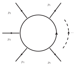
Figure 1: One-loop N-point diagram.

We consider a set of external momenta ${k_{1},\dots,k_{N}}$ which satisfy momentum conservation $\sum_{i=1}^{N}k_{i}=0$. Inverse propagators can be defined as

$$\mathcal{D}_{i}={(\ell+r_{i})}^{2}-m_{i}^{2},\quad i=1,\dots,N\ ,$$ (13)

where $\ell$ is loop momentum, the momenta $r_{i}$ are defined by $r_{i}=k_{i}+r_{i-1}$ for $i=1,\dots,N$, and $r_{0}=r_{N}=0$ by definition. For the sake of clarity, we omit the infinitesimal imaginary part $\mathrm{i}\epsilon$ in inverse propagators, since the reductions are independent of it. As there is no ISP at the one-loop level, we introduce GFs as

$$G_{\vec{\nu}}(\vec{\eta})=\int\frac{\mathrm{d}^{D}\ell}{\mathrm{i}\pi^{D/2}}\frac{1}{\prod_{i=1}^{N}({\cal D}_{i}-\eta_{i})^{\nu_{i}}},$$ (14)

and MIs of GFs can be chosen as that with $\nu_{i}$ being $0$ or $1$. The IBP equations

$$\int\frac{\mathrm{d}^{D}\ell}{\mathrm{i}\pi^{D/2}}\frac{\partial}{\partial\ell^{\mu}}\frac{\ell^{\mu}+r_{i}^{\mu}}{\prod_{j=1}^{N}({\cal D}_{j}-\eta_{j})}=0,\quad i=1,\dots,N\ ,$$ (15)

lead to DEs of GFs:

$$\begin{split}&\sum_{j=1}^{N}(R_{ji}-\eta_{j}-\eta_{i})\frac{\partial G_{\text{top}}}{\partial\eta_{j}}\\ &=\sum_{j\neq i}^{N}\frac{\partial G_{\text{top}-\vec{e}_{i}}}{\partial\eta_{j}}+(1-D+N)G_{\text{top}},\end{split}$$ (16)

where $R_{ji}=(r_{j}-r_{i})^{2}-m_{i}^{2}-m_{j}^{2}$ is the Gram matrix of the one-loop N-point family, $\vec{e}_{i}$ with $i=1,\dots,N$ are unit vectors and “$\text{top}-\vec{e}_{i}$” means “$(1,\cdots,1)-\vec{e}_{i}$”.

By expanding Eq.(16) at small value of $\vec{\eta}$, the coefficients of $\prod_{k=1}^{N}\eta_{k}^{\nu_{k}-1}$ result in

$$\begin{split}&\sum_{j=1}^{N}R_{ji}\nu_{j}I(\{\nu_{k}+\delta_{kj}\})=\\ &\sum_{j=1}^{N}\nu_{j}I(\{\nu_{k}+\delta_{kj}-\delta_{ki}\})-(D-\sum_{j=1}^{N}\nu_{j})I(\{\nu_{k}\}),\end{split}$$ (17)

which can reduce all FIs with nonzero dots to MIs. Therefore, we find that the DEs of GFs provide all desired recurrence relations at one-loop level. Our result is consistent with that presented in Eq.(1) of Ref. [142].

Furthermore, by expanding Eq.(16) at small value of $1/\eta_{i}$ for some index $i$ and small value of $\eta_{i}$ for the others, we can gain the same recurrence relations in Eq. (17), which can reduce FIs with negative powers. FIs with negative powers can also be viewed as tensor integrals, which can be related to scalar integrals via Lorentz decomposition [143]. Alternatively, the tensor integrals can also be reduced by GFs with auxiliary vector [136].

IV Two-loop sunrise

Now let us give a simple two-loop example, the massless sunrise family shown in Fig.2. The family has two loop momenta $\ell_{1}$ and $\ell_{2}$ and one external momenta $k$, satisfying $k^{2}=s$. We choose a complete set of Lorentz scalars as

$$\begin{split}&\mathcal{D}_{1}={\ell_{1}}^{2},\mathcal{D}_{2}={\ell_{2}}^{2},\mathcal{D}_{3}={(\ell_{1}+\ell_{2}+k)}^{2},\\ &\mathcal{D}_{4}=\ell_{1}\cdot k,\mathcal{D}_{5}=\ell_{2}\cdot k,\end{split}$$ (18)

where the last two are ISPs. We choose the ISPs as products of loop momenta and external momenta, instead of quadratic forms like $(\ell_{1}+k)^{2}$, since the former have simpler DEs in practice.

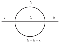
Figure 2: Two-loop sunrise diagram.

Although we can construct DEs w.r.t $x_{i}$ and $\eta_{i}$ to obtain recurrence relations to reduce all FIs in the family, this is not necessary. Instead, reduction problems can be usually divided into two cases: 1) with large rank but small dots; 2) with large dots but small rank. We thus will only deal with these two cases.

Considering arbitrary powers of ISPs, we choose GFs defined in Eq. (9):

$$G_{\vec{\nu}}(\vec{x})=\int\frac{\mathrm{d}^{D}\ell_{1}\mathrm{d}^{D}\ell_{2}}{(\mathrm{i}\pi^{D/2})^{2}}\frac{\mathcal{D}_{4}^{-\nu_{4}}\mathcal{D}_{5}^{-\nu_{5}}e^{Z^{\vec{x}}}}{\mathcal{D}_{1}^{\nu_{1}}\mathcal{D}_{2}^{\nu_{2}}\mathcal{D}_{3}^{\nu_{3}}},$$ (19)

where ${\nu_{4},\nu_{5}}$ are non-positive integers only. MIs can be chosen as

$$\vec{\cal{G}}=\left(G_{(1,1,1,0,0)},G_{(1,1,1,0,-1)},G_{(1,1,1,-1,0)}\right),$$ (20)

which include only top-sector integrals because all sub-sector integrals in this family are scaleless and vanishing in dimensional regularization. Using Blade, we get the DEs w.r.t. $x_{i}$:

$$\frac{\partial}{\partial x_{i}}\vec{\cal{G}}=A_{i}\;\vec{\cal{G}},$$ (21)

where

$$A_{4}=\begin{pmatrix}0&1&0\\ \frac{(-1+\epsilon)s}{x_{4}}&\frac{(-1+\epsilon)(3x_{4}-2x_{5})}{x_{4}(x_{4}-x_{5})}-\frac{s}{2}&-\frac{(-1+\epsilon)x_{5}}{x_{4}(x_{4}-x_{5})}\\ -\frac{s^{2}}{4}&-\frac{-1+\epsilon}{x_{4}-x_{5}}-\frac{s}{2}&\frac{-1+\epsilon}{x_{4}-x_{5}}-\frac{s}{2}\end{pmatrix},$$ (22)

$$A_{5}=\begin{pmatrix}0&0&1\\ -\frac{s^{2}}{4}&-\frac{-1+\epsilon}{x_{4}-x_{5}}-\frac{s}{2}&\frac{-1+\epsilon}{x_{4}-x_{5}}-\frac{s}{2}\\ \frac{(-1+\epsilon)s}{x_{5}}&\frac{(-1+\epsilon)x_{4}}{x_{5}(x_{4}-x_{5})}&\frac{(-1+\epsilon)(2x_{4}-3x_{5})}{x_{5}(x_{4}-x_{5})}-\frac{s}{2}\end{pmatrix},$$ (23)

By expanding the DEs to $x_{4}^{\nu_{4}}x_{5}^{\nu_{5}}$ with arbitrary $\nu_{4}$ and $\nu_{5}$, we obtain three different linear relations between FIs. Due to the permutation symmetry of the sunrise FIs, $I(\nu_{4},\nu_{5})\equiv I(1,1,1,\nu_{4},\nu_{5})=I(1,1,1,\nu_{5},\nu_{4})$, we only need to consider the cases where $\nu_{4}\leq\nu_{5}\leq 0$ and thus we have the following relation:

$$\begin{split}&c_{0}I(\nu_{4},\nu_{5})\\ =&c_{1}I(1+\nu_{4},\nu_{5})+c_{2}I(1+\nu_{4},1+\nu_{5})+c_{3}I(2+\nu_{4},\nu_{5}),\end{split}$$ (24)

where

$$\begin{split}c_{0}&=4(-1+2\epsilon+\nu_{4})[(\nu_{5}-1)(\nu_{4}+\nu_{5}-2)\\ &+\epsilon(\nu_{4}^{2}-\nu_{5}^{2}+7\nu_{5}-7)+3\epsilon^{2}(2+\nu_{4}-\nu_{5})],\\ c_{1}&=-2s[(\nu_{4}^{3}+\nu_{4}^{2}(2\nu_{5}-3)+\nu_{4}(1-\nu_{5})+(\nu_{5}-1)^{2})\\ &+\epsilon(\nu_{4}^{3}+\nu_{4}^{2}(8-\nu_{5})+2\nu_{4}(3\nu_{5}-5)-(\nu_{5}-1)(2\nu_{5}-5))\\ &+\epsilon^{2}(2\nu_{4}^{2}+\nu_{4}(19-3\nu_{5})+(5-\nu_{5})(1-\nu_{5}))\\ &+\epsilon^{3}2(1-\nu_{4}+\nu_{5})],\\ c_{2}&=-s^{2}(-1+\epsilon)(-1+2\epsilon+\nu_{4})\nu_{5}(-1+2\epsilon+\nu_{5}),\\ c_{3}&=-s^{2}(1+\nu_{4})(2\epsilon+\nu_{4})(\nu_{4}+\nu_{5}-2-\epsilon(\nu_{5}-5)-2\epsilon^{2}),\\ \end{split}$$

This recurrence relation can reduce $I(\nu_{4},\nu_{5})$ with $\nu_{4}\leq\nu_{5}\leq 0$ to $I(0,0)$. Note that, as Eq. (24) is an analytic function of $\nu_{4}$ and $\nu_{5}$, it also holds even if $\nu_{4}$ and $\nu_{5}$ are positive.

To obtain the reduction of arbitrary powers of propagators with no ISP, we introduce GFs:

$$\begin{split}&G_{\vec{\nu}}(\vec{\eta})=\\ &\int\frac{\mathrm{d}^{D}\ell_{1}\mathrm{d}^{D}\ell_{2}}{(\mathrm{i}\pi^{D/2})^{2}}\frac{1}{(\mathcal{D}_{1}-\eta_{1})^{\nu_{1}}(\mathcal{D}_{2}-\eta_{2})^{\nu_{2}}(\mathcal{D}_{3}-\eta_{3})^{\nu_{3}}}.\end{split}$$ (25)

MIs can be effectively chosen as

$$\vec{\cal{G}}=\left(G_{(1,1,1)},G_{(2,1,1)},G_{(1,2,1)},G_{(1,1,2)}\right),$$

because the expansion coefficients of $G_{\vec{\nu}}(\vec{\eta})$ are scaleless if any $\nu_{i}\leq 0$. The DEs of $\vec{\cal{G}}$ w.r.t. $\eta_{i}$ and the corresponding recurrence relations can be similarly obtained, which are available in the ancillary file.

V Two-loop double-box

In this section, we take the double-box diagram shown in Fig.3 as an example to demonstrate that: 1) the fixed direction scheme is usually preferred; and 2) the construction of DEs of GFs is usually much easier than the construction of recurrence relations of original FIs directly.

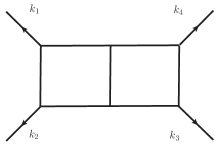
Figure 3: Two-loop double-box diagram.

In this problem, there are four external momenta $k_{1}$, $k_{2}$, $k_{3}$, $k_{4}$ satisfying on-shell conditions $k_{i}^{2}=0$ and momentum conservation $\sum_{i=1}^{4}k_{i}=0$, which leaves two independent scales $s=2k_{1}\cdot k_{2}$ and $t=2k_{2}\cdot k_{3}$. We choose a complete set of Lorentz scalars as

$$\begin{split}&\mathcal{D}_{1}={\ell_{1}}^{2},\ \mathcal{D}_{2}=(\ell_{1}+k_{1})^{2},\ \mathcal{D}_{3}={(\ell_{1}+k_{1}+k_{2})}^{2},\\ &\mathcal{D}_{4}={\ell_{2}}^{2},\ \mathcal{D}_{5}={(\ell_{2}-\ell_{1})}^{2},\ \mathcal{D}_{6}={(\ell_{2}+k_{1}+k_{2})}^{2},\\ &\mathcal{D}_{7}={(\ell_{2}-k_{4})}^{2},\ \mathcal{D}_{8}=\ell_{1}\cdot k_{3},\ \mathcal{D}_{9}=\ell_{2}\cdot k_{1},\end{split}$$ (26)

where the last two are ISPs. DEs of GFs in this family are too long to present, and they are available in the ancillary file.

V.1 Fixed direction scheme

Based on GFs defined in Eq. (9), there are 108 MIs with 5 in the top-sector. We construct DEs of these MIs w.r.t. variables $x_{i}$ ($i=8,9$),

$$\frac{\partial}{\partial x_{i}}\vec{\cal G}= A_{i}\vec{\cal G}\ ,$$ (27)

and find that there are many singularities in the coefficient matrices. For example, the matrix elements $(A_{8})_{6,6}$, associated with $\partial_{x_{8}}G_{(0,0,1,1,1,0,0,-1,-1)}$ and $G_{(0,0,1,1,1,0,0,-1,-1)}$, possesses a denominator

$$\text{den}((A_{8})_{6,6})= 2x_{8}\times(sx_{8}^{2}+2sx_{8}x_{9}+2tx_{8}x_{9}+sx_{9}^{2})$$

$$\times (sx_{8}^{2}+2sx_{8}x_{9}+4tx_{8}x_{9}+sx_{9}^{2})\ .$$ (28)

The complicated denominators lead to complicated numerators, and thus large number of numeric sample points are required to reconstruct the matrix $A_{i}$. Therefore, it is very time-consuming.

Alternatively, we can choose the fixed direction scheme defined in Eq. (11). In this scheme there are the same number of MIs as the previous scheme, but DEs w.r.t $x$,

$$\frac{\partial}{\partial x}\vec{\cal G}^{\vec{c}}= A^{\vec{c}}\vec{\cal G}^{\vec{c}},$$ (29)

are much simpler. For example, by choosing $c_{8}=1$ and $c_{9}=2$, the denominator of the matrix element $(A^{(1,2)}_{x})_{6,6}$ becomes

$$\text{den}((A^{(1,2)}_{x})_{6,6})=2x(9s+4t),$$ (30)

which results in also simpler numerators. In fact, for any given value of $\vec{c}$, one can always choose MIs of GFs so that $A^{\vec{c}}$ only has singularities at $x=0$ and $x=\infty$, and thus the construction of $A^{\vec{c}}$ is much easier than that of $A_{i}$ in Eq. (27). As shown in Tab. 1, construction of $A_{i}$, which are functions of $s,~{}t,~{}\epsilon,~{}x_{8}$ and $x_{9}$, needs 130 seconds CPU time; while the construction of $A^{\vec{c}}$ with given value of $\vec{c}$, which are functions of $s,~{}t,~{}\epsilon$ and $x$, needs 13 seconds.

Scheme	#MIs	$t_{\text{ibp}}$(s)	Points	Primes	$t_{\text{total}}$(s)
all	108	0.02	3307	2	130
fixed direction	108	0.02	324	2	13 $\times(r+1)/3$

Table 1: Comparing the GFs method with all variables scheme and fixed direction scheme. #MIs represents the number of MIs of GFs. $t_{\text{ibp}}$ represents CPU time to solve the trimmed numeric IBP system. Points represents number of numeric sample points to fit $\vec{s}$, $\epsilon$ and $\vec{x}$. Primes represents number of large prime for rational reconstruction. $t_{\text{total}}$ represents total CPU time of IBP reduction for constructing DEs of GFs.

However, to reduce top-sector FIs with rank $r$, which amounts to $r+1$ FIs, in the fixed direction scheme we need to sample $\vec{c}$ for $(r+1)/3$ times. This is because we find that, for each given value of $\vec{c}$, DEs of GFs can provide 3 linearly independent relations among top-sector FIs with highest rank. Therefore, when rank $r<29$, which is much larger than rank of FIs in usual physical problems, the efficiency of the fixed direction scheme is better.

V.2 Comparison with constructing recurrence relations directly

We note that using Blade one can reduce FIs with arbitrary powers of ISPs to lower powers, and thus construct recurrence relations directly. It is necessary to compare the efficiency between this direct way and the way based on GFs. To this end, we introduce FIs with arbitrary powers of ISPs:

$$I_{\vec{\nu}}(n_{1},n_{2})=\int\frac{\mathrm{d}^{D}\ell_{1}\mathrm{d}^{D}\ell_{2}}{(\mathrm{i}\pi^{D/2})^{2}}\frac{\mathcal{D}_{8}^{n_{1}}\mathcal{D}_{9}^{n_{2}}}{\prod_{i=1}^{7}{\cal D}_{i}^{\nu_{i}}},$$ (31)

where the ISPs $\{\mathcal{D}_{8},\ \mathcal{D}_{9}\}$ could be linear form: $\{\ell_{1}\cdot k_{3},\ \ell_{2}\cdot k_{1}\}$, or quadratic form: $\{(\ell_{1}+k_{3})^{2},\ (\ell_{2}+k_{1})^{2}\}$.

Using Blade, we can achieve the reduction of FIs, like reducing $I_{\vec{\nu}}(n_{1}+1,n_{2})$ and $I_{\vec{\nu}}(n_{1},n_{2}+1)$ to $I_{\vec{\nu}}(n_{1},n_{2})$, which are the desired recurrence relations. The CPU time to achieve recurrence relations in this way is shown in Tab.2, which is clear less efficient comparing with the GFs method shown in Tab. 1. This comparison indicates the superiority of GF for generating recurrence relations.

Form	#MIs	$t_{\text{ibp}}$(s)	Points	Primes	$t_{\text{total}}$(s)
linear	60	0.07	20139	3	4220
quadratic	63	0.14	8031	2	2300

Table 2: Comparison of constructing recurrence relations using IBP reduction directly with different choices of ISPs (linear or quadratic form). #MIs represents the number of MIs of FIs with general powers. Points represents the number of numeric sample points to fit variables $\vec{s}$, $\epsilon$ and $\vec{n}$. Other information are the same as that in Tab.1.

VI Two-loop double-pentagon

In this section, we use the GFs method to deal with a cutting-edge problem, the massless two-loop double-pentagon family shown in Fig.4. The reduction of FIs in this family up to rank 5, which are relevant for five-light-parton scattering amplitudes in QCD, has been previously accomplished [28, 39, 144]. There are five external momenta $k_{1}$, $k_{2}$, $k_{3}$, $k_{4}$, $k_{5}$ satisfying on-shell conditions $k_{i}^{2}=0$ and momentum conservation $\sum_{i=1}^{5}k_{i}=0$, leaving five kinematic variables $s_{12}=k_{1}\cdot k_{2}$, $s_{23}=k_{2}\cdot k_{3}$, $s_{13}=k_{1}\cdot k_{3}$, $s_{14}=k_{1}\cdot k_{4}$, $s_{34}=k_{3}\cdot k_{4}$ as the mass scales. We choose a complete set of Lorentz scalars as

$$\begin{split}&\mathcal{D}_{1}={\ell_{1}}^{2},\ \mathcal{D}_{2}=(\ell_{1}+k_{1})^{2},\ \mathcal{D}_{3}={(\ell_{1}+k_{1}+k_{2})}^{2},\\ &\mathcal{D}_{4}={\ell_{2}}^{2},\ \mathcal{D}_{5}={(\ell_{2}-\ell_{1})}^{2},\ \mathcal{D}_{6}={(l_{2}-l_{1}+k_{5})}^{2},\\ &\mathcal{D}_{7}={(\ell_{2}-k_{3}-k_{4})}^{2},\ \mathcal{D}_{8}={(\ell_{2}-k_{4})}^{2},\\ &\mathcal{D}_{9}=\ell_{1}\cdot k_{3},\ \mathcal{D}_{10}=\ell_{2}\cdot k_{1},\ \mathcal{D}_{11}=\ell_{2}\cdot k_{2},\end{split}$$ (32)

where the last three are ISPs.

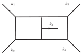
Figure 4: Two-loop double-pentagon diagram.

MIs	$t_{\text{ibp}}$(s)	$\text{Mem}_{\text{ibp}}$(GB)	Points	Number of $\vec{c}$
(4,0)	4.9	12.4	32	$(2+r)(1+r)/24$
(0,2)	3.6	2.7	108	$(2+r)(1+r)/2$

Table 3: Information for reducing double-pentagon FIs using GFs method. MIs represents the max (rank,dots) of different choices of master integrals. $t_{\text{ibp}}$ represents the time spent to solve trimmed IBP system numerically for one time. $\text{Mem}_{\text{ibp}}$ represents the memory used to load and trim the raw IBP system, usually the maximal memory consumption in the calculation. Points means number of numeric sample points of $x$ to reconstruct $x$-dependence of DEs per $\vec{c}$. Number of $\vec{c}$ represents the number of samples of $\vec{c}$ needed to reduce rank $r$ FIs.

To reduce powers of ISPs, we define the following GFs

$$G_{\vec{\nu}}^{\vec{c}}(x)=\int\frac{\mathrm{d}^{D}\ell_{1}\mathrm{d}^{D}\ell_{2}}{(\mathrm{i}\pi^{D/2})^{2}}\frac{e^{xZ^{\vec{c}}}}{\prod_{i=1}^{11}{\cal D}_{i}^{\nu_{i}}}.$$ (33)

There are 908 MIs of these GFs in total and 18 MIs in the top sector. MIs in the top sector can be chosen as

$$\begin{split}\{&G_{(1,\dots,1,0,0,0)}^{\vec{c}},\ G_{(1,\dots,1,-1,0,0)}^{\vec{c}},\ G_{(1,\dots,1,0,-1,0)}^{\vec{c}},\\ &G_{(1,\dots,1,0,0,-1)}^{\vec{c}},\ G_{(1,\dots,1,-1,-1,0)}^{\vec{c}},\ G_{(1,\dots,1,-1,0,-1)}^{\vec{c}},\\ &G_{(1,\dots,1,0,-1,-1)}^{\vec{c}},\ G_{(1,\dots,1,-2,0,0)}^{\vec{c}},\ G_{(1,\dots,1,0,-2,0)}^{\vec{c}},\\ &G_{(1,\dots,1,0,0,-2)}^{\vec{c}},\ G_{(1,\dots,1,-1,-1,-1)}^{\vec{c}},\ G_{(1,\dots,1,-2,0,-1)}^{\vec{c}},\\ &G_{(1,\dots,1,-1,-2,0)}^{\vec{c}},\ G_{(1,\dots,1,-1,0,-2)}^{\vec{c}},\ G_{(1,\dots,1,0,-2,-1)}^{\vec{c}},\\ &G_{(1,\dots,1,0,-1,-2)}^{\vec{c}},\ G_{(1,\dots,1,0,-2,-2)}^{\vec{c}},\ G_{(1,\dots,1,-2,-2,0)}^{\vec{c}}\},\end{split}$$

which is denoted as $(4,0)$-type because the max rank is 4 and max dot is 0. Alternatively, MIs can be chosen as

$$\begin{split}\{&G_{(1,1,1,1,1,1,1,1,0,0,0)}^{\vec{c}},\quad G_{(1,1,1,1,1,1,1,2,0,0,0)}^{\vec{c}},\\ &G_{(1,1,1,1,1,2,1,1,0,0,0)}^{\vec{c}},\quad G_{(1,1,1,1,2,1,1,1,0,0,0)}^{\vec{c}},\\ &G_{(1,1,1,2,1,1,1,1,0,0,0)}^{\vec{c}},\quad G_{(1,1,2,1,1,1,1,1,0,0,0)}^{\vec{c}},\\ &G_{(1,2,1,1,1,1,1,1,0,0,0)}^{\vec{c}},\quad G_{(2,1,1,1,1,1,1,1,0,0,0)}^{\vec{c}},\\ &G_{(1,2,1,1,1,2,1,1,0,0,0)}^{\vec{c}},\quad G_{(1,2,1,2,1,1,1,1,0,0,0)}^{\vec{c}},\\ &G_{(1,2,2,1,1,1,1,1,0,0,0)}^{\vec{c}},\quad G_{(2,1,1,1,1,1,1,2,0,0,0)}^{\vec{c}},\\ &G_{(2,1,1,1,1,2,1,1,0,0,0)}^{\vec{c}},\quad G_{(2,1,1,1,2,1,1,1,0,0,0)}^{\vec{c}},\\ &G_{(2,1,1,2,1,1,1,1,0,0,0)}^{\vec{c}},\quad G_{(2,2,1,1,1,1,1,1,0,0,0)}^{\vec{c}},\\ &G_{(1,3,1,1,1,1,1,1,0,0,0)}^{\vec{c}},\quad G_{(3,1,1,1,1,1,1,1,0,0,0)}^{\vec{c}}\},\end{split}$$

which is denoted as $(0,2)$-type because the max rank is 0 and max dot is 2.

Using Blade, we set up closed DEs of these MIs w.r.t $x$. As shown in Tab.3, to reduce each point (i.e., given values of kinematic variables, $\epsilon$, $\vec{c}$ and $x$), it costs $4.9~{}(3.6)$ seconds and uses memory up to $12.4~{}(2.7)$ GB, respectively for $(4,0)$-type and $(0,2)$-type. To fully construct the $x$ dependence of the DEs, we need to simulate 32 or 108 different values of $x$, respectively. Furthermore, to reduce top-sector integrals with rank $r$, we need to simulate $(2+r)(1+r)/24$ or $(2+r)(1+r)/2$ different choices of $\vec{c}$, respectively.

rank	$t_{\text{ibp}}$(s)	$\text{Mem}_{ibp}$(GB)
4	1.4	2.8
5	3.9	7.0
6	11	15.8
7	29	33.2
8	66	65.6

Table 4: Information for reducing double-pentagon FIs using plain IBP method. $t_{\text{ibp}}$ represents the time spent to solve IBP system numerically using one CPU. Mem_ibp represents the maximal memory consumption in solving the IBP system.

As a comparison, in Tab.4 we present the time and resource consumption for reducing FIs in the double-pentagon family with different ranks using IBP method directly. It is clear that the memory used in IBP method increases fast as the rank becoming larger. In contrast, in the GFs method, the memory is a constant value, independent of the rank of the target FIs to be reduced. In this example, when $r>4$, the GFs method with the MIs type (0,2) needs smaller memory.

For each point, the time consumption in the GFs method is compatible with the IBP method for $r=5$. This is understandable because, to construct the DEs of GFs with the MIs type (4,0), one needs to reduce rank 5 GFs to lower ranks. However, because currently 32 points are needed to reconstruct the $x$-dependent DEs, the total CPU time $32\times 4.9\times(2+r)(1+r)/24$, is still too long. As there are only two singularities $x=0$ or $\infty$ in the $x$ plane, which are respectively regular singularity and essential singularity, it is possible to find a better set of MIs so that the DEs are in a canonical form

$$\frac{\partial}{\partial x}\vec{\cal G}^{\vec{c}}= \left(\frac{C_{1}^{\vec{c}}}{x}+C_{0}^{\vec{c}}\right)\vec{\cal G}^{\vec{c}},$$ (34)

where $C_{1}^{\vec{c}}$ and $C_{0}^{\vec{c}}$ are independent of $x$. When the DEs of the MIs satisfy the canonical form, only two points of $x$ are needed to fully reconstruct the DEs instead of 32 points. In this case, the CPU time cost by the GFs method is $2\times 4.9\times(2+r)(1+r)/24$, comparable with that of IBP method when $r=7$ and the GFs method with the MIs type (4,0) becomes more efficient when $r>7$.

Note that the DEs of sunrise family in Eq. (21) are already in the canonical form if we set $x_{i}=xc_{i}$. For general cases, we will study the construction of canonical DEs of GFs in future publications.

VII Summary and outlook

In this paper, we have introduced a general method for constructing recurrence relations of Feynman integrals (FIs) using generating functions (GFs). We have demonstrated that by formulating and solving the differential equations (DEs) associated with GFs, we can effectively reduce FIs within a given family.

Compared to the plain IBP method, the GFs method proves to be significantly more efficient for constructing recurrence relations. When it comes to reducing FIs with specific ranks, the GFs method offers advantages in terms of time and resource consumption, particularly when the rank is large. However, for smaller ranks, the GFs method may not provide the same level of efficiency. This aspect makes the GFs method particularly appealing for addressing high-rank problems, such as effective field theory problems, like the calculation of twist-two operator matrix elements in QCD, and gravitational scattering problems. For example, in the calculation of Mellin Moments of splitting function by twist-two operator matrix elements, the rank of Feynman Integrals is $O(20)$ at four-loop level in planar limit [145] and that is $O(500)$ or higher for the full three-loop contribution [133, 134, 135].

An important aspect to study is the selection of appropriate bases that lead to DEs of GFs in a canonical form defined in Eq. (34). Techniques developed in recent years for constructing $\epsilon$-forms of FIs [84] could potentially be useful in this context, although further investigation is necessary.

Given that we employ IBP relations to construct DEs of GFs, any advancements in IBP reduction techniques would also benefit our method. One possible direction is to integrate the syzygy method with the GFs method, utilizing the latter to handle the reduction of sub-sector integrals. By doing so, the DEs of GFs in the top sector can be derived with the assistance of DEs of GFs in the sub-sectors. This integration of techniques enables us to fully harness the capabilities of the GFs method, resulting in more efficient computations.

VIII Acknowledgements

We thank B. Feng, L.H. Huang, M. Zeng, T.Z.Yang for many useful communications and discussions. The work was supported in part by the National Natural Science Foundation of China (Grants No. 11875071, No. 11975029), the National Key Research and Development Program of China under Contracts No. 2020YFA0406400, and the High-performance Computing Platform of Peking University. JaxoDraw [146] was used to generate Feynman diagrams.

References

- [1] P. Azzi et al., Report from Working Group 1: Standard Model Physics at the HL-LHC and HE-LHC, CERN Yellow Rep. Monogr. 7 (2019) 1–220 [arXiv:1902.04070] [InSPIRE].
- [2] M. Cepeda et al., Report from Working Group 2: Higgs Physics at the HL-LHC and HE-LHC, CERN Yellow Rep. Monogr. 7 (2019) 221–584 [arXiv:1902.00134] [InSPIRE].
- [3] ILC , The International Linear Collider Technical Design Report - Volume 2: Physics, [arXiv:1306.6352] [InSPIRE].
- [4] The International Linear Collider Technical Design Report - Volume 1: Executive Summary, [arXiv:1306.6327] [InSPIRE].
- [5] P. Bambade et al., The International Linear Collider: A Global Project, [arXiv:1903.01629] [InSPIRE].
- [6] CEPC Study Group , M. Dong et al., CEPC Conceptual Design Report: Volume 2 - Physics & Detector, [arXiv:1811.10545] [InSPIRE].
- [7] CEPC Study Group , CEPC Conceptual Design Report: Volume 1 - Accelerator, [arXiv:1809.00285] [InSPIRE].
- [8] TLEP Design Study Working Group , M. Bicer et al., First Look at the Physics Case of TLEP, JHEP 01 (2014) 164 [arXiv:1308.6176] [InSPIRE].
- [9] FCC , A. Abada et al., FCC Physics Opportunities: Future Circular Collider Conceptual Design Report Volume 1, Eur. Phys. J. C 79 (2019) 474 [InSPIRE].
- [10] FCC , A. Abada et al., FCC-ee: The Lepton Collider: Future Circular Collider Conceptual Design Report Volume 2, Eur. Phys. J. ST 228 (2019) 261–623 [InSPIRE].
- [11] A. V. Smirnov and A. V. Petukhov, The Number of Master Integrals is Finite, Lett. Math. Phys. 97 (2011) 37–44 [arXiv:1004.4199] [InSPIRE].
- [12] K. G. Chetyrkin and F. V. Tkachov, Integration by Parts: The Algorithm to Calculate beta Functions in 4 Loops, Nucl. Phys. B 192 (1981) 159–204 [InSPIRE].
- [13] T. Gehrmann and E. Remiddi, Differential equations for two loop four point functions, Nucl. Phys. B 580 (2000) 485–518 [hep-ph/9912329] [InSPIRE].
- [14] S. Laporta, High precision calculation of multiloop Feynman integrals by difference equations, Int. J. Mod. Phys. A 15 (2000) 5087–5159 [hep-ph/0102033] [InSPIRE].
- [15] P. A. Baikov, A Practical criterion of irreducibility of multi-loop Feynman integrals, Phys. Lett. B 634 (2006) 325–329 [hep-ph/0507053] [InSPIRE].
- [16] P. A. Baikov, Recurrence relations in the large space-time dimension limit, PoS RADCOR2007 (2007) 022 [InSPIRE].
- [17] J. Gluza, K. Kajda, and D. A. Kosower, Towards a Basis for Planar Two-Loop Integrals, Phys. Rev. D 83 (2011) 045012 [arXiv:1009.0472] [InSPIRE].
- [18] R. M. Schabinger, A New Algorithm For The Generation Of Unitarity-Compatible Integration By Parts Relations, JHEP 01 (2012) 077 [arXiv:1111.4220] [InSPIRE].
- [19] K. J. Larsen and Y. Zhang, Integration-by-parts reductions from unitarity cuts and algebraic geometry, Phys. Rev. D 93 (2016) 041701 [arXiv:1511.01071] [InSPIRE].
- [20] Z. Wu, J. Boehm, R. Ma, H. Xu, and Y. Zhang, NeatIBP 1.0, A package generating small-size integration-by-parts relations for Feynman integrals, [arXiv:2305.08783] [InSPIRE].
- [21] A. von Manteuffel and R. M. Schabinger, A novel approach to integration by parts reduction, Phys. Lett. B 744 (2015) 101–104 [arXiv:1406.4513] [InSPIRE].
- [22] T. Peraro, Scattering amplitudes over finite fields and multivariate functional reconstruction, JHEP 12 (2016) 030 [arXiv:1608.01902] [InSPIRE].
- [23] T. Peraro, FiniteFlow: multivariate functional reconstruction using finite fields and dataflow graphs, JHEP 07 (2019) 031 [arXiv:1905.08019] [InSPIRE].
- [24] J. Klappert and F. Lange, Reconstructing rational functions with FireFly, Comput. Phys. Commun. 247 (2020) 106951 [arXiv:1904.00009] [InSPIRE].
- [25] J. Klappert, S. Y. Klein, and F. Lange, Interpolation of dense and sparse rational functions and other improvements in FireFly, Comput. Phys. Commun. 264 (2021) 107968 [arXiv:2004.01463] [InSPIRE].
- [26] A. V. Belitsky, A. V. Smirnov, and R. V. Yakovlev, Balancing act: multivariate rational reconstruction for IBP, [arXiv:2303.02511] [InSPIRE].
- [27] X. Liu and Y.-Q. Ma, Determining arbitrary Feynman integrals by vacuum integrals, Phys. Rev. D 99 (2019) 071501 [arXiv:1801.10523] [InSPIRE].
- [28] X. Guan, X. Liu, and Y.-Q. Ma, Complete reduction of integrals in two-loop five-light-parton scattering amplitudes, Chin. Phys. C 44 (2020) 093106 [arXiv:1912.09294] [InSPIRE].
- [29] https://gitlab.com/multiloop-pku/blade.
- [30] A. V. Smirnov and V. A. Smirnov, How to choose master integrals, Nucl. Phys. B 960 (2020) 115213 [arXiv:2002.08042] [InSPIRE].
- [31] J. Usovitsch, Factorization of denominators in integration-by-parts reductions, [arXiv:2002.08173] [InSPIRE].
- [32] C. Anastasiou and A. Lazopoulos, Automatic integral reduction for higher order perturbative calculations, JHEP 07 (2004) 046 [hep-ph/0404258] [InSPIRE].
- [33] A. V. Smirnov, Algorithm FIRE – Feynman Integral REduction, JHEP 10 (2008) 107 [arXiv:0807.3243] [InSPIRE].
- [34] A. V. Smirnov and V. A. Smirnov, FIRE4, LiteRed and accompanying tools to solve integration by parts relations, Comput. Phys. Commun. 184 (2013) 2820–2827 [arXiv:1302.5885] [InSPIRE].
- [35] A. V. Smirnov, FIRE5: a C++ implementation of Feynman Integral REduction, Comput. Phys. Commun. 189 (2015) 182–191 [arXiv:1408.2372] [InSPIRE].
- [36] A. V. Smirnov and F. S. Chuharev, FIRE6: Feynman Integral REduction with Modular Arithmetic, Comput. Phys. Commun. 247 (2020) 106877 [arXiv:1901.07808] [InSPIRE].
- [37] P. Maierhöfer, J. Usovitsch, and P. Uwer, Kira—A Feynman integral reduction program, Comput. Phys. Commun. 230 (2018) 99–112 [arXiv:1705.05610] [InSPIRE].
- [38] P. Maierhöfer and J. Usovitsch, Kira 1.2 Release Notes, [arXiv:1812.01491] [InSPIRE].
- [39] J. Klappert, F. Lange, P. Maierhöfer, and J. Usovitsch, Integral reduction with Kira 2.0 and finite field methods, Comput. Phys. Commun. 266 (2021) 108024 [arXiv:2008.06494] [InSPIRE].
- [40] R. N. Lee, Presenting LiteRed: a tool for the Loop InTEgrals REDuction, [arXiv:1212.2685] [InSPIRE].
- [41] R. N. Lee, LiteRed 1.4: a powerful tool for reduction of multiloop integrals, J. Phys. Conf. Ser. 523 (2014) 012059 [arXiv:1310.1145] [InSPIRE].
- [42] C. Studerus, Reduze-Feynman Integral Reduction in C++, Comput. Phys. Commun. 181 (2010) 1293–1300 [arXiv:0912.2546] [InSPIRE].
- [43] A. von Manteuffel and C. Studerus, Reduze 2 - Distributed Feynman Integral Reduction, [arXiv:1201.4330] [InSPIRE].
- [44] P. Mastrolia and S. Mizera, Feynman Integrals and Intersection Theory, JHEP 02 (2019) 139 [arXiv:1810.03818] [InSPIRE].
- [45] H. Frellesvig, F. Gasparotto, S. Laporta, M. K. Mandal, P. Mastrolia, L. Mattiazzi, and S. Mizera, Decomposition of Feynman Integrals on the Maximal Cut by Intersection Numbers, JHEP 05 (2019) 153 [arXiv:1901.11510] [InSPIRE].
- [46] H. Frellesvig, F. Gasparotto, S. Laporta, M. K. Mandal, P. Mastrolia, L. Mattiazzi, and S. Mizera, Decomposition of Feynman Integrals by Multivariate Intersection Numbers, JHEP 03 (2021) 027 [arXiv:2008.04823] [InSPIRE].
- [47] S. Weinzierl, On the computation of intersection numbers for twisted cocycles, J. Math. Phys. 62 (2021) 072301 [arXiv:2002.01930] [InSPIRE].
- [48] Y. Wang, Z. Li, and N. Ul Basat, Direct reduction of multiloop multiscale scattering amplitudes, Phys. Rev. D 101 (2020) 076023 [arXiv:1901.09390] [InSPIRE].
- [49] J. Boehm, M. Wittmann, Z. Wu, Y. Xu, and Y. Zhang, IBP reduction coefficients made simple, JHEP 12 (2020) 054 [arXiv:2008.13194] [InSPIRE].
- [50] N. u. Basat, Z. Li, and Y. Wang, Reduction of the planar double-box diagram for single-top production via auxiliary mass flow, Phys. Rev. D 104 (2021) 056020 [arXiv:2102.08225] [InSPIRE].
- [51] M. Heller and A. von Manteuffel, MultivariateApart: Generalized partial fractions, Comput. Phys. Commun. 271 (2022) 108174 [arXiv:2101.08283] [InSPIRE].
- [52] D. Bendle, J. Boehm, M. Heymann, R. Ma, M. Rahn, L. Ristau, M. Wittmann, Z. Wu, and Y. Zhang, pfd-parallel, a Singular/GPI-Space package for massively parallel multivariate partial fractioning, [arXiv:2104.06866] [InSPIRE].
- [53] K. Hepp, Proof of the Bogolyubov-Parasiuk theorem on renormalization, Commun. Math. Phys. 2 (1966) 301–326 [InSPIRE].
- [54] M. Roth and A. Denner, High-energy approximation of one loop Feynman integrals, Nucl. Phys. B 479 (1996) 495–514 [hep-ph/9605420] [InSPIRE].
- [55] T. Binoth and G. Heinrich, An automatized algorithm to compute infrared divergent multiloop integrals, Nucl. Phys. B 585 (2000) 741–759 [hep-ph/0004013] [InSPIRE].
- [56] G. Heinrich, Sector Decomposition, Int. J. Mod. Phys. A 23 (2008) 1457–1486 [arXiv:0803.4177] [InSPIRE].
- [57] A. V. Smirnov and M. N. Tentyukov, Feynman Integral Evaluation by a Sector decomposiTion Approach (FIESTA), Comput. Phys. Commun. 180 (2009) 735–746 [arXiv:0807.4129] [InSPIRE].
- [58] A. V. Smirnov, V. A. Smirnov, and M. Tentyukov, FIESTA 2: Parallelizeable multiloop numerical calculations, Comput. Phys. Commun. 182 (2011) 790–803 [arXiv:0912.0158] [InSPIRE].
- [59] A. V. Smirnov, FIESTA 3: cluster-parallelizable multiloop numerical calculations in physical regions, Comput. Phys. Commun. 185 (2014) 2090–2100 [arXiv:1312.3186] [InSPIRE].
- [60] A. V. Smirnov, FIESTA4: Optimized Feynman integral calculations with GPU support, Comput. Phys. Commun. 204 (2016) 189–199 [arXiv:1511.03614] [InSPIRE].
- [61] A. V. Smirnov, N. D. Shapurov, and L. I. Vysotsky, FIESTA5: Numerical high-performance Feynman integral evaluation, Comput. Phys. Commun. 277 (2022) 108386 [arXiv:2110.11660] [InSPIRE].
- [62] J. Carter and G. Heinrich, SecDec: A general program for sector decomposition, Comput. Phys. Commun. 182 (2011) 1566–1581 [arXiv:1011.5493] [InSPIRE].
- [63] S. Borowka, J. Carter, and G. Heinrich, Numerical Evaluation of Multi-Loop Integrals for Arbitrary Kinematics with SecDec 2.0, Comput. Phys. Commun. 184 (2013) 396–408 [arXiv:1204.4152] [InSPIRE].
- [64] S. Borowka, G. Heinrich, S. P. Jones, M. Kerner, J. Schlenk, and T. Zirke, SecDec-3.0: numerical evaluation of multi-scale integrals beyond one loop, Comput. Phys. Commun. 196 (2015) 470–491 [arXiv:1502.06595] [InSPIRE].
- [65] S. Borowka, G. Heinrich, S. Jahn, S. P. Jones, M. Kerner, J. Schlenk, and T. Zirke, pySecDec: a toolbox for the numerical evaluation of multi-scale integrals, Comput. Phys. Commun. 222 (2018) 313–326 [arXiv:1703.09692] [InSPIRE].
- [66] S. Borowka, G. Heinrich, S. Jahn, S. P. Jones, M. Kerner, and J. Schlenk, A GPU compatible quasi-Monte Carlo integrator interfaced to pySecDec, Comput. Phys. Commun. 240 (2019) 120–137 [arXiv:1811.11720] [InSPIRE].
- [67] M. C. Bergere and Y.-M. P. Lam, ASYMPTOTIC EXPANSION OF FEYNMAN AMPLITUDES. Part 1: THE CONVERGENT CASE, Commun. Math. Phys. 39 (1974) 1 [InSPIRE].
- [68] E. E. Boos and A. I. Davydychev, A Method of evaluating massive Feynman integrals, Theor. Math. Phys. 89 (1991) 1052–1063 [InSPIRE].
- [69] V. A. Smirnov, Analytical result for dimensionally regularized massless on shell double box, Phys. Lett. B 460 (1999) 397–404 [hep-ph/9905323] [InSPIRE].
- [70] J. B. Tausk, Nonplanar massless two loop Feynman diagrams with four on-shell legs, Phys. Lett. B 469 (1999) 225–234 [hep-ph/9909506] [InSPIRE].
- [71] M. Czakon, Automatized analytic continuation of Mellin-Barnes integrals, Comput. Phys. Commun. 175 (2006) 559–571 [hep-ph/0511200] [InSPIRE].
- [72] A. V. Smirnov and V. A. Smirnov, On the Resolution of Singularities of Multiple Mellin-Barnes Integrals, Eur. Phys. J. C 62 (2009) 445–449 [arXiv:0901.0386] [InSPIRE].
- [73] J. Gluza, K. Kajda, and T. Riemann, AMBRE: A Mathematica package for the construction of Mellin-Barnes representations for Feynman integrals, Comput. Phys. Commun. 177 (2007) 879–893 [arXiv:0704.2423] [InSPIRE].
- [74] https://mbtools.hepforge.org/.
- [75] A. V. Belitsky, A. V. Smirnov, and V. A. Smirnov, MB Tools reloaded, [arXiv:2211.00009] [InSPIRE].
- [76] M. Beneke and V. A. Smirnov, Asymptotic expansion of Feynman integrals near threshold, Nucl. Phys. B 522 (1998) 321–344 [hep-ph/9711391] [InSPIRE].
- [77] B. Jantzen, A. V. Smirnov, and V. A. Smirnov, Expansion by regions: revealing potential and Glauber regions automatically, Eur. Phys. J. C 72 (2012) 2139 [arXiv:1206.0546] [InSPIRE].
- [78] R. N. Lee, Space-time dimensionality D as complex variable: Calculating loop integrals using dimensional recurrence relation and analytical properties with respect to D, Nucl. Phys. B 830 (2010) 474–492 [arXiv:0911.0252] [InSPIRE].
- [79] A. V. Kotikov, Differential equations method: New technique for massive Feynman diagrams calculation, Phys. Lett. B 254 (1991) 158–164 [InSPIRE].
- [80] A. V. Kotikov, Differential equation method: The Calculation of N point Feynman diagrams, Phys. Lett. B 267 (1991) 123–127 [InSPIRE]. [Erratum: Phys.Lett.B 295, 409–409 (1992)].
- [81] E. Remiddi, Differential equations for Feynman graph amplitudes, Nuovo Cim. A 110 (1997) 1435–1452 [hep-th/9711188] [InSPIRE].
- [82] M. Argeri and P. Mastrolia, Feynman Diagrams and Differential Equations, Int. J. Mod. Phys. A 22 (2007) 4375–4436 [arXiv:0707.4037] [InSPIRE].
- [83] S. Müller-Stach, S. Weinzierl, and R. Zayadeh, Picard-Fuchs equations for Feynman integrals, Commun. Math. Phys. 326 (2014) 237–249 [arXiv:1212.4389] [InSPIRE].
- [84] J. M. Henn, Multiloop integrals in dimensional regularization made simple, Phys. Rev. Lett. 110 (2013) 251601 [arXiv:1304.1806] [InSPIRE].
- [85] J. M. Henn, Lectures on differential equations for Feynman integrals, J. Phys. A 48 (2015) 153001 [arXiv:1412.2296] [InSPIRE].
- [86] F. Moriello, Generalised power series expansions for the elliptic planar families of Higgs + jet production at two loops, JHEP 01 (2020) 150 [arXiv:1907.13234] [InSPIRE].
- [87] M. Hidding, DiffExp, a Mathematica package for computing Feynman integrals in terms of one-dimensional series expansions, Comput. Phys. Commun. 269 (2021) 108125 [arXiv:2006.05510] [InSPIRE].
- [88] T. Armadillo, R. Bonciani, S. Devoto, N. Rana, and A. Vicini, Evaluation of Feynman integrals with arbitrary complex masses via series expansions, Comput. Phys. Commun. 282 (2023) 108545 [arXiv:2205.03345] [InSPIRE].
- [89] S. Catani, T. Gleisberg, F. Krauss, G. Rodrigo, and J.-C. Winter, From loops to trees by-passing Feynman’s theorem, JHEP 09 (2008) 065 [arXiv:0804.3170] [InSPIRE].
- [90] I. Bierenbaum, S. Catani, P. Draggiotis, and G. Rodrigo, A Tree-Loop Duality Relation at Two Loops and Beyond, JHEP 10 (2010) 073 [arXiv:1007.0194] [InSPIRE].
- [91] I. Bierenbaum, S. Buchta, P. Draggiotis, I. Malamos, and G. Rodrigo, Tree-Loop Duality Relation beyond simple poles, JHEP 03 (2013) 025 [arXiv:1211.5048] [InSPIRE].
- [92] E. T. Tomboulis, Causality and Unitarity via the Tree-Loop Duality Relation, JHEP 05 (2017) 148 [arXiv:1701.07052] [InSPIRE].
- [93] R. Runkel, Z. Szőr, J. P. Vesga, and S. Weinzierl, Causality and loop-tree duality at higher loops, Phys. Rev. Lett. 122 (2019) 111603 [arXiv:1902.02135] [InSPIRE]. [Erratum: Phys.Rev.Lett. 123, 059902 (2019)].
- [94] Z. Capatti, V. Hirschi, D. Kermanschah, and B. Ruijl, Loop-Tree Duality for Multiloop Numerical Integration, Phys. Rev. Lett. 123 (2019) 151602 [arXiv:1906.06138] [InSPIRE].
- [95] J. J. Aguilera-Verdugo, F. Driencourt-Mangin, R. J. Hernández-Pinto, J. Plenter, S. Ramirez-Uribe, A. E. Renteria Olivo, G. Rodrigo, G. F. R. Sborlini, W. J. Torres Bobadilla, and S. Tracz, Open Loop Amplitudes and Causality to All Orders and Powers from the Loop-Tree Duality, Phys. Rev. Lett. 124 (2020) 211602 [arXiv:2001.03564] [InSPIRE].
- [96] F. C. Brown, On the periods of some Feynman integrals, [arXiv:0910.0114] [InSPIRE].
- [97] E. Panzer, Feynman integrals and hyperlogarithms. PhD thesis, Humboldt U., 2015 [arXiv:1506.07243] [InSPIRE].
- [98] E. Panzer, Algorithms for the symbolic integration of hyperlogarithms with applications to Feynman integrals, Comput. Phys. Commun. 188 (2015) 148–166 [arXiv:1403.3385] [InSPIRE].
- [99] M. Hidding and J. Usovitsch, Feynman parameter integration through differential equations, [arXiv:2206.14790] [InSPIRE].
- [100] X. Liu, Y.-Q. Ma, and C.-Y. Wang, A Systematic and Efficient Method to Compute Multi-loop Master Integrals, Phys. Lett. B 779 (2018) 353–357 [arXiv:1711.09572] [InSPIRE].
- [101] X. Liu, Y.-Q. Ma, W. Tao, and P. Zhang, Calculation of Feynman loop integration and phase-space integration via auxiliary mass flow, Chin. Phys. C 45 (2021) 013115 [arXiv:2009.07987] [InSPIRE].
- [102] X. Liu and Y.-Q. Ma, Multiloop corrections for collider processes using auxiliary mass flow, Phys. Rev. D 105 (2022) L051503 [arXiv:2107.01864] [InSPIRE].
- [103] X. Liu and Y.-Q. Ma, AMFlow: A Mathematica package for Feynman integrals computation via auxiliary mass flow, Comput. Phys. Commun. 283 (2023) 108565 [arXiv:2201.11669] [InSPIRE].
- [104] Z.-F. Liu and Y.-Q. Ma, Automatic computation of Feynman integrals containing linear propagators via auxiliary mass flow, Phys. Rev. D 105 (2022) 074003 [arXiv:2201.11636] [InSPIRE].
- [105] Z.-F. Liu and Y.-Q. Ma, Determining Feynman Integrals with Only Input from Linear Algebra, Phys. Rev. Lett. 129 (2022) 222001 [arXiv:2201.11637] [InSPIRE].
- [106] Q. Song and A. Freitas, On the evaluation of two-loop electroweak box diagrams for production, JHEP 04 (2021) 179 [arXiv:2101.00308] [InSPIRE].
- [107] M. Zeng, Feynman Integrals from Positivity Constraints, [arXiv:2303.15624] [InSPIRE].
- [108] D. Cabarcas and J. Ding, Linear algebra to compute syzygies and gröbner bases, in Proceedings of the 36th International Symposium on Symbolic and Algebraic Computation, ISSAC ’11, p. 67–74. Association for Computing Machinery, New York, NY, USA, 2011 [InSPIRE]. https://doi.org/10.1145/1993886.1993902.
- [109] H. Ita, Two-loop Integrand Decomposition into Master Integrals and Surface Terms, Phys. Rev. D 94 (2016) 116015 [arXiv:1510.05626] [InSPIRE].
- [110] Y. Zhang, Lecture Notes on Multi-loop Integral Reduction and Applied Algebraic Geometry, 12, 2016 [arXiv:1612.02249] [InSPIRE].
- [111] J. Böhm, A. Georgoudis, K. J. Larsen, H. Schönemann, and Y. Zhang, Complete integration-by-parts reductions of the non-planar hexagon-box via module intersections, JHEP 09 (2018) 024 [arXiv:1805.01873] [InSPIRE].
- [112] A. von Manteuffel, E. Panzer, and R. M. Schabinger, Cusp and collinear anomalous dimensions in four-loop QCD from form factors, Phys. Rev. Lett. 124 (2020) 162001 [arXiv:2002.04617] [InSPIRE].
- [113] S. Badger, C. Brønnum-Hansen, D. Chicherin, T. Gehrmann, H. B. Hartanto, J. Henn, M. Marcoli, R. Moodie, T. Peraro, and S. Zoia, Virtual QCD corrections to gluon-initiated diphoton plus jet production at hadron colliders, JHEP 11 (2021) 083 [arXiv:2106.08664] [InSPIRE].
- [114] S. Abreu, F. Febres Cordero, H. Ita, M. Klinkert, B. Page, and V. Sotnikov, Leading-color two-loop amplitudes for four partons and a W boson in QCD, JHEP 04 (2022) 042 [arXiv:2110.07541] [InSPIRE].
- [115] F. V. Tkachov, AN ALGORITHM FOR CALCULATING MULTILOOP INTEGRALS, Theor. Math. Phys. 56 (1983) 866–870 [InSPIRE].
- [116] N. Gray, D. J. Broadhurst, W. Grafe, and K. Schilcher, Three Loop Relation of Quark (Modified) Ms and Pole Masses, Z. Phys. C 48 (1990) 673–680 [InSPIRE].
- [117] D. J. Broadhurst and A. G. Grozin, Two loop renormalization of the effective field theory of a static quark, Phys. Lett. B 267 (1991) 105–110 [hep-ph/9908362] [InSPIRE].
- [118] A. I. Davydychev and J. B. Tausk, Two loop selfenergy diagrams with different masses and the momentum expansion, Nucl. Phys. B 397 (1993) 123–142 [InSPIRE].
- [119] M. Caffo, H. Czyz, S. Laporta, and E. Remiddi, The Master differential equations for the two loop sunrise selfmass amplitudes, Nuovo Cim. A 111 (1998) 365–389 [hep-th/9805118] [InSPIRE].
- [120] K. Melnikov and T. v. Ritbergen, The Three loop relation between the MS-bar and the pole quark masses, Phys. Lett. B 482 (2000) 99–108 [hep-ph/9912391] [InSPIRE].
- [121] M. Steinhauser, MATAD: A Program package for the computation of MAssive TADpoles, Comput. Phys. Commun. 134 (2001) 335–364 [hep-ph/0009029] [InSPIRE].
- [122] S. G. Gorishnii, S. A. Larin, L. R. Surguladze, and F. V. Tkachov, Mincer: Program for Multiloop Calculations in Quantum Field Theory for the Schoonschip System, Comput. Phys. Commun. 55 (1989) 381–408 [InSPIRE].
- [123] S. A. Larin, F. V. Tkachov, and J. A. M. Vermaseren, The FORM version of MINCER, [InSPIRE].
- [124] B. Ruijl, T. Ueda, and J. A. M. Vermaseren, Forcer, a FORM program for the parametric reduction of four-loop massless propagator diagrams, Comput. Phys. Commun. 253 (2020) 107198 [arXiv:1704.06650] [InSPIRE].
- [125] O. V. Tarasov, Computation of Grobner bases for two loop propagator type integrals, Nucl. Instrum. Meth. A 534 (2004) 293–298 [hep-ph/0403253] [InSPIRE].
- [126] V. P. Gerdt and D. Robertz, A Maple package for computing Grobner bases for linear recurrence relations, Nucl. Instrum. Meth. A 559 (2006) 215–219 [cs/0509070] [InSPIRE].
- [127] A. V. Smirnov and V. A. Smirnov, Applying Grobner bases to solve reduction problems for Feynman integrals, JHEP 01 (2006) 001 [hep-lat/0509187] [InSPIRE].
- [128] A. V. Smirnov, An Algorithm to construct Grobner bases for solving integration by parts relations, JHEP 04 (2006) 026 [hep-ph/0602078] [InSPIRE].
- [129] A. V. Smirnov and V. A. Smirnov, S-bases as a tool to solve reduction problems for Feynman integrals, Nucl. Phys. B Proc. Suppl. 160 (2006) 80–84 [hep-ph/0606247] [InSPIRE].
- [130] R. N. Lee, Group structure of the integration-by-part identities and its application to the reduction of multiloop integrals, JHEP 07 (2008) 031 [arXiv:0804.3008] [InSPIRE].
- [131] M. Barakat, R. Brüser, C. Fieker, T. Huber, and J. Piclum, Feynman integral reduction using Gröbner bases, [arXiv:2210.05347] [InSPIRE].
- [132] J. Ablinger, J. Blümlein, A. De Freitas, A. Hasselhuhn, S. Klein, C. Schneider, and F. Wißbrock, New Results on the 3-Loop Heavy Flavor Wilson Coefficients in Deep-Inelastic Scattering, PoS ICHEP2012 (2013) 270 [arXiv:1212.5950] [InSPIRE].
- [133] J. Blümlein, P. Marquard, C. Schneider, and K. Schönwald, The three-loop unpolarized and polarized non-singlet anomalous dimensions from off shell operator matrix elements, Nucl. Phys. B 971 (2021) 115542 [arXiv:2107.06267] [InSPIRE].
- [134] J. Blümlein, P. Marquard, C. Schneider, and K. Schönwald, The three-loop polarized singlet anomalous dimensions from off-shell operator matrix elements, JHEP 01 (2022) 193 [arXiv:2111.12401] [InSPIRE].
- [135] T. Gehrmann, A. von Manteuffel, and T.-Z. Yang, Renormalization of twist-two operators in covariant gauge to three loops in QCD, JHEP 04 (2023) 041 [arXiv:2302.00022] [InSPIRE].
- [136] B. Feng, Generation Function For One-loop Tensor Reduction, [arXiv:2209.09517] [InSPIRE].
- [137] B. Feng, T. Li, and X. Li, Analytic tadpole coefficients of one-loop integrals, JHEP 09 (2021) 081 [arXiv:2107.03744] [InSPIRE].
- [138] C. Hu, T. Li, and X. Li, One-loop Feynman integral reduction by differential operators, Phys. Rev. D 104 (2021) 116014 [arXiv:2108.00772] [InSPIRE].
- [139] B. Feng and T. Li, PV-reduction of sunset topology with auxiliary vector, Commun. Theor. Phys. 74 (2022) 095201 [arXiv:2203.16881] [InSPIRE].
- [140] B. Feng, C. Hu, T. Li, and Y. Song, Reduction with degenerate Gram matrix for one-loop integrals, JHEP 08 (2022) 110 [arXiv:2205.03000] [InSPIRE].
- [141] B. Feng, T. Li, H. Wang, and Y. Zhang, Reduction of general one-loop integrals using auxiliary vector, JHEP 05 (2022) 065 [arXiv:2203.14449] [InSPIRE].
- [142] G. Duplancic and B. Nizic, Reduction method for dimensionally regulated one loop N point Feynman integrals, Eur. Phys. J. C 35 (2004) 105–118 [hep-ph/0303184] [InSPIRE].
- [143] G. Passarino and M. J. G. Veltman, One Loop Corrections for e+ e- Annihilation Into mu+ mu- in the Weinberg Model, Nucl. Phys. B 160 (1979) 151–207 [InSPIRE].
- [144] B. Agarwal, F. Buccioni, A. von Manteuffel, and L. Tancredi, Two-Loop Helicity Amplitudes for Diphoton Plus Jet Production in Full Color, Phys. Rev. Lett. 127 (2021) 262001 [arXiv:2105.04585] [InSPIRE].
- [145] S. Moch, B. Ruijl, T. Ueda, J. A. M. Vermaseren, and A. Vogt, Four-Loop Non-Singlet Splitting Functions in the Planar Limit and Beyond, JHEP 10 (2017) 041 [arXiv:1707.08315] [InSPIRE].
- [146] D. Binosi and L. Theussl, JaxoDraw: A Graphical user interface for drawing Feynman diagrams, Comput. Phys. Commun. 161 (2004) 76–86 [hep-ph/0309015] [InSPIRE].