Decentralized SGD and Average-direction SAM are Asymptotically Equivalent

Abstract

Decentralized stochastic gradient descent (D-SGD) allows collaborative learning on massive devices simultaneously without the control of a central server. However, existing theories claim that decentralization invariably undermines generalization. In this paper, we challenge this conventional belief and present a completely new perspective for understanding decentralized learning. We prove that D-SGD implicitly minimizes the loss function of an average-direction sharpness-aware minimization (SAM) algorithm under general non-convex non-$\beta$-smooth settings. This surprising asymptotic equivalence reveals an intrinsic regularization-optimization trade-off and three advantages of decentralization: (1) there exists a free uncertainty evaluation mechanism in D-SGD to improve posterior estimation; (2) D-SGD exhibits a gradient smoothing effect; and (3) the sharpness regularization effect of D-SGD does not decrease as total batch size increases, which justifies the potential generalization benefit of D-SGD over centralized SGD (C-SGD) in large-batch scenarios. Experiments support our theory and the code is available at  D-SGD and SAM.

1 Introduction

Decentralized training harnesses the power of locally connected computing resources while preserving privacy (Warnat-Herresthal et al., 2021; Borzunov et al., 2022; Yuan et al., 2022; Beltrán et al., 2022; Lu & Sa, 2023). Decentralized stochastic gradient descent (D-SGD) is a popular decentralized training algorithm which enables simultaneous model training on a massive number of workers without the need for a central server (Xiao & Boyd, 2004; Lopes & Sayed, 2008; Nedic & Ozdaglar, 2009; Lian et al., 2017; Koloskova et al., 2020). In D-SGD, each worker communicates only with its directly connected neighbors; see a detailed background in Subsection A.2. This decentralization avoids the requirements of a costly central server with heavy communication burdens and potential privacy risks. The existing literature demonstrates that the massive models on edge can converge to a steady consensus model (Lu et al., 2011; Shi et al., 2015), with asymptotic linear speedup in convergence rate (Lian et al., 2017) similar to distributed centralized SGD (C-SGD) (Dean et al., 2012; Li et al., 2014). Therefore, D-SGD offers a promising distributed learning solution with significant advantages in communication efficiency (Ying et al., 2021b), privacy (Nedic, 2020) and scalability (Lian et al., 2017).

Despite these merits, it is regrettable that the existing theories claim decentralization to invariably undermines generalization (Sun et al., 2021; Zhu et al., 2022; Deng et al., 2023), which contradicts the following unique phenomena in decentralized deep learning:

• D-SGD can outperform C-SGD in large-batch settings, achieving higher validation accuracy and smaller validation-training accuracy gap, despite both being fine-tuned (Zhang et al., 2021);

• A non-negligible consensus distance (see Eq. 3) at middle phases of decentralized training can improve generalization over centralized training (Kong et al., 2021).

These unexplained phenomena indicates the existence of a non-negligible Gap between existing theories and deep learning experiments, which we attribute to the overlook of important characteristics of decentralized learning in existing literature. Accordingly, the primary Goal of our study is to thoroughly investigate the underexamined characteristics of decentralized learning, in an effort to to bridge the gap.

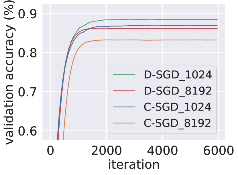
((a)) AlexNet

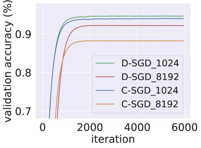
((b)) ResNet-18

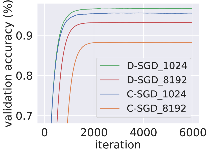
((c)) DenseNet-121

Figure 1: The validation accuracy comparison of C-SGD and D-SGD (ring topology) on CIFAR-10. The number of workers is set as 16, with a local batch size of 64 and 512 per worker, resulting in total batch sizes of 1024 and 8192, respectively. Validation accuracy comparison of C-SGD and D-SGD with other topologies and on Tiny ImageNet are included in Figure B.1 and Figure B.2, respectively. The training accuracy is almost $100\%$ everywhere. Exponential moving average is employed to smooth the validation accuracy curves. The training setting is included in Appendix B.

Directly analyzing the dynamics of the diffusion-like decentralized learning systems, instead of relying on upper bounds, can be challenging. Instead, we aim to establish a relationship between D-SGD and other centralized training algorithms. In recent years, there has been a growing interest in techniques that aim to improve the generalization of deep learning models. One of the most popular techniques is sharpness-aware minimization (SAM) (Foret et al., 2021; Kwon et al., 2021; Zhuang et al., 2022; Du et al., 2022; Kim et al., 2022), which is designed to explicitly minimize a sharpness-based perturbed loss; see the detailed background of SAM in Subsection A.3. Empirical studies have shown that SAM substantially improves the generalization of multiple architectures, including convolutional neural networks (Wu et al., 2020; Foret et al., 2021), vision transformers (Dosovitskiy et al., 2021) and large language models (Bahri et al., 2022). Average-direction SAM (Wen et al., 2023), a kind of SAM variants where sharpness is calculated as the (weighted) average within a small neighborhood around the current iterate, has been shown to generalize on par with vanilla SAM (Ujváry et al., 2022).

In this paper, we provide a completely new perspective for understanding decentralized learning by showing that

Specifically, our contributions are summarized below.

• We prove that D-SGD asymptotically minimizes the loss function of an average-direction sharpness-aware minimization algorithm with zero additional computation (see Theorem 1), which directly connects decentralized training and centralized training. The asymptotic equivalence also implies a regularization-optimization trade-off in decentralized training. Our theory is applicable to arbitrary communication topologies (see Definition A.1) and general non-convex and non-$\beta$-smooth (see Definition A.5) objectives (e.g., deep neural networks training).

• The equivalence further reveals the potential benefits of the decentralized training paradigm, which challenges the previously held belief that centralized training is optimal. We demonstrate three advantages of training with decentralized models based on the equivalence: (1) there exists a surprising free uncertainty estimation mechanism in D-SGD, where the weight diversity matrix $\bm{\Xi}{\scriptstyle(t)}$ is learned to estimate $\Sigma_{q}$, the intractable covariance of the posterior;(2) D-SGD has a gradient smoothing effect, which improves training stability (see Corollary 2); and that (3) the sharpness regularizer of D-SGD does not decrease as the total batch size increases (see Theorem 3), which justifies the superior generalizability of D-SGD than C-SGD, especially in large-batch settings where gradient variance remains low. Our empirical results also fully support our theory (see Figure 1 and Figure 3).

To the best of our knowledge, our work is the first to establish the equivalence of D-SGD and average-direction SAM, which constitutes a direct connection between decentralized training and centralized training algorithms. This breakthrough makes it easier to analyze the diffusion-like decentralized systems, whose exact dynamics were considered challenging to understand. The theory further sheds light on the potential benefits of decentralized training paradigm. While our theory primarily focuses on vanilla D-SGD, it could be directly extended to general decentralized gradient-based algorithms. We anticipate the insights derived from our work will help bridge the decentralized learning and SAM communities, and pave the way for the development of fast and generalizable decentralized algorithms.

2 Related work

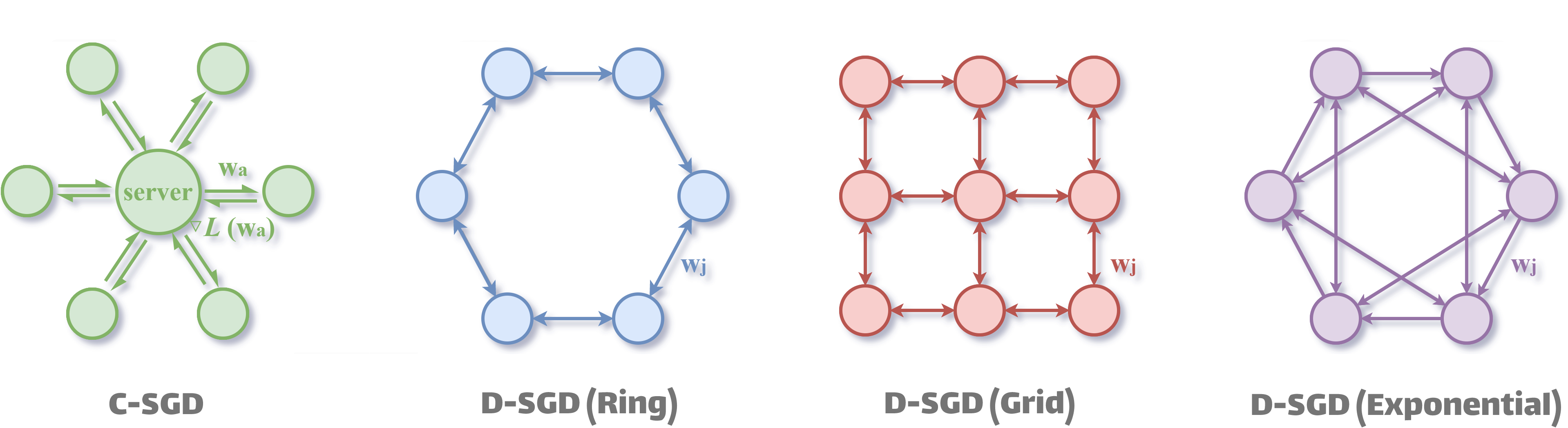
Figure 2: An illustration of centralized SGD and decentralized SGD. In C-SGD there is a central server aggregating global information while D-SGD relies only on peer-to-peer communication to diffuse information among workers.

Flatness and generalization. The flatness of the minimum has long been regarded as a proxy of generalization in the machine learning literature (Hochreiter & Schmidhuber, 1997; Neyshabur et al., 2017; Izmailov et al., 2018; Jiang et al., 2020). Intuitively, the loss around a flat minimum varies slowly in a large neighborhood, while a sharp minimum increases rapidly in a small neighborhood (Hochreiter & Schmidhuber, 1997). Through the lens of the minimum description length theory (Rissanen, 1983), flat minimizers, due to their specification with lower precision, tend to generalize better than sharp minimizers (Keskar et al., 2017). From a Bayesian perspective, sharp minimizers have highly concentrated posterior parameter distributions, indicating a greater specialization to the training set and thus are less robust to data perturbations than flat minimizers (MacKay, 1992; Chaudhari et al., 2019).

Generalization of D-SGD. Recently works by Sun et al. (2021), Zhu et al. (2022) and Deng et al. (2023) prove that decentralization introduces an additional positive term into the generalization error bounds, which suggests that decentralization may hurt generalization. However, these conservative upper bounds do not account for the unique phenomena in decentralized learning, such as the superior generalization performance of D-SGD in large batch scenarios. Gurbuzbalaban et al. (2022) offers an alternative perspective, showing that D-SGD with large, sparse topology has a heavier tail in parameter distribution than C-SGD in some cases, indicating better generalizability potential. Compared with Gurbuzbalaban et al. (2022), our theory is generally applicable to arbitrary communication topologies and learning rates. Another work by Zhang et al. (2021) demonstrates that decentralization introduces a landscape-dependent noise, which may improve the convergence of D-SGD. However, the impact of noise on the local geometry of the D-SGD trajectory and its effect on generalization remains unexplored. In contrast, we theoretically justify the flatness-seeking behavior of Hessian-dependent noise in D-SGD and then establish the asymptotic equivalence between D-SGD and SAM. Based on the equivalence, we prove that D-SGD has superior potential in generalizability compared with C-SGD, especially in large-batch settings.

3 Preliminaries

Basic notations. Suppose that $\mathcal{X}\subseteq\mathbb{R}^{d_{x}}$ and $\mathcal{Y}\subseteq\mathbb{R}$ are the input and output spaces, respectively. We denote the training set as $\mu=\left\{z_{1},\ldots,z_{N}\right\}$, where $z_{\zeta}=\left(x_{\zeta},y_{\zeta}\right),\zeta=1,\dots,N$ are sampled independent and identically distributed (i.i.d.) from an unknown data distribution $\mathcal{D}$ defined on $\mathcal{Z}=\mathcal{X}\times\mathcal{Y}$. The goal of supervised learning is to learn a predictor (or hypothesis) $g(\mathbf{w};\cdot)$, parameterized by $\mathbf{w}\in\mathbb{R}^{d}$ of an arbitrary finite dimension $d$, to approximate the mapping between the input variable $x\in\mathcal{X}$ and the output variable $y\in\mathcal{Y}$, based on the training set $\mu$. The function $c:\mathcal{Y}\times\mathcal{Y}\mapsto\mathbb{R}^{+}$ are defined to evaluate the prediction performance of hypothesis $g$. The loss of a hypothesis $g$ with respect to (w.r.t.) the example $z_{\zeta}=(x_{\zeta},y_{\zeta})$ is denoted by ${\bm{L}}(\mathbf{w};z_{\zeta})=c(g(\mathbf{w};x_{\zeta}),y_{\zeta})$, which measures the effectiveness of the learned model $\mathbf{w}$. The empirical and population risks of $\mathbf{w}$ are then defined as follows:

$${\bm{L}}^{\mu}_{\mathbf{w}}=\frac{1}{N}\sum_{\zeta=1}^{N}{\bm{L}}(\mathbf{w};z_{\zeta}),~{}~{}{\bm{L}}_{\mathbf{w}}=\mathbb{E}_{z\sim D}[{\bm{L}}(\mathbf{w};z)].$$

Distributed learning. Distributed learning trains a model $\mathbf{w}$ jointly using multiple workers (Shamir & Srebro, 2014). In this framework, the $j$-th worker $(j\scalebox{0.75}[1.0]{$=$}1,\dots,m)$ can access local training examples $\mu_{j}\scalebox{0.75}[1.0]{$=$}\{z_{j,1},\ldots,z_{j,|\mu_{j}|}\}$, drawn from the local empirical distribution $\mathcal{D}_{j}$. In this setup, the global empirical risk of $\mathbf{w}$ becomes

$${\bm{L}}^{\mu}_{\mathbf{w}}=\frac{1}{m}\sum_{j=1}^{m}{\bm{L}}^{\mu_{j}}_{\mathbf{w}},$$

where ${\bm{L}}^{\mu_{j}}_{\mathbf{w}}=\frac{1}{|\mu_{j}|}\sum_{\zeta=1}^{|\mu_{j}|}{\bm{L}}({\mathbf{w}};z_{j,\zeta})$ denotes the local empirical risk on the $j$-th worker and $z_{j,\zeta}\in\mu_{j}$, where $\zeta=1,\dots,|\mu_{j}|$, represent the local training data.

Distributed centralized stochastic gradient descent (C-SGD). In C-SGD (Dean et al., 2012; Li et al., 2014), the de facto distributed training algorithm, there is only one centralized model $\mathbf{w}_{a}{\scriptstyle(t)}$. C-SGD updates the model by

$$\mathbf{w}_{a}{\scriptstyle(t+1)}=\mathbf{w}_{a}{\scriptstyle(t)}-\eta\cdot\frac{1}{m}\sum_{j=1}^{m}\overbrace{\nabla{\bm{L}}^{\mu_{j}{\scriptstyle(t)}}(\mathbf{w}_{a}{\scriptstyle(t)})}^{\text{Local gradient computation}},$$ (1)

where $\eta$ denotes the learning rate (step size), $\mu_{j}{\scriptstyle(t)}=\{z_{j,1},\ldots,z_{j,|\mu_{j}{\scriptstyle(t)}|}\}$ denotes the local training batch independent and identically distributed (i.i.d.) drawn from the local empirical data distribution $\mathcal{D}_{j}$ at the $t$-th iteration, and $\nabla{\bm{L}}^{\mu_{j}{\scriptstyle(t)}}_{\mathbf{w}}=\nabla{\bm{L}}^{\mu_{j}{\scriptstyle(t)}}(\mathbf{w})=\frac{1}{|\mu_{j}{\scriptstyle(t)}|}\sum_{\zeta{\scriptstyle(t)}=1}^{|\mu_{j}{\scriptstyle(t)}|}\nabla{\bm{L}}({\mathbf{w}};z_{j,\zeta{\scriptstyle(t)}})$ stacks for the local mini-batch gradient of ${\bm{L}}$ w.r.t. the first argument $\mathbf{w}$. The total batch size of C-SGD at the $t$-th iteration is $|\mu{\scriptstyle(t)}|=\sum_{j=1}^{m}|\mu_{j}{\scriptstyle(t)}|$. Please refer to Subsection A.1 for more details of (distributed) centralized learning. In the next section, we will show that C-SGD equals the single-worker SGD with a larger batch size.

Decentralized stochastic gradient descent (D-SGD). In model decentralization scenarios, only peer-to-peer communication is allowed. The goal of D-SGD in the setup is to learn a consensus model $\mathbf{w}_{a}{\scriptstyle(t)}=\frac{1}{m}\sum_{j=1}^{m}\mathbf{w}_{j}{\scriptstyle(t)}$ on $m$ workers through gossip communication, where $\mathbf{w}_{j}{\scriptstyle(t)}$ stands for the $d$-dimensional local model on the $j$-th worker. We denote ${\mathbf{P}}=[\mathbf{P}_{j,k}]\in\mathbb{R}^{m\times m}$ as a doubly stochastic gossip matrix (see Definition A.1) that characterizes the underlying topology $\mathcal{G}$. The vanilla Adapt-While-Communicate (AWC) version of the mini-batch D-SGD (Nedic & Ozdaglar, 2009; Lian et al., 2017) updates the model on the $j$-th worker by

$$\mathbf{w}_{j}{\scriptstyle(t+1)}=\overbrace{\sum_{k=1}^{m}\mathbf{P}_{j,k}\mathbf{w}_{k}{\scriptstyle(t)}}^{\text{Communication}}-\eta\cdot\overbrace{\nabla{\bm{L}}^{\mu_{j}{\scriptstyle(t)}}(\mathbf{w}_{j}{\scriptstyle(t)})}^{\text{Local gradient computation}}.$$ (2)

For a more detailed background of decentralized learning, please kindly refer to Subsection A.2.

4 Theoretical results

In this section, we establish the equivalence between D-SGD and average-direction SAM under general non-convex and non-$\beta$-smooth objectives ${\bm{L}}$. We also provide a proof sketch to offer a more intuitive understanding. The equivalence further showcases the potential superiority of learning with decentralized models. Specifically, we prove that the additional noise introduced by decentralization leads to a gradient smoothing effect, which could stabilize optimization. Additionally, we show that the sharpness regularizer in D-SGD does not decrease as the total batch size increases, which guarantees generalizability in large-batch settings.

4.1 Equivalences of Decentralized SGD and average-direction SAM

In this subsection, we prove that D-SGD implicitly performs average-direction sharpness-aware minimization (SAM), followed by detailed implications.

Theorem 1 (D-SGD as SAM).

Suppose ${\bm{L}}\in C^{4}\left(\mathbb{R}^{d}\right)$, i.e., ${\bm{L}}$ is four times continuously differentiable. The mean iterate of the global averaged model of D-SGD, defined by $\mathbf{w}_{a}{\scriptstyle(t)}=\frac{1}{m}\sum_{j=1}^{m}\mathbf{w}_{j}{\scriptstyle(t)}$, is provided as follows:

$$\mathbb{E}_{\mu{\scriptscriptstyle(t)}} [\mathbf{w}_{a}{\scriptstyle(t+1)}]$$

$$= \mathbf{w}_{a}{\scriptstyle(t)}-\eta\color[rgb]{0,0,0.7}{\underbrace{\color[rgb]{0,0,0}{\mathchoice{\leavevmode\hbox to75.89pt{\vbox to11pt{\text{[drawing]}}}}{\leavevmode\hbox to75.89pt{\vbox to11pt{\text{[drawing]}}}}{\leavevmode\hbox to53.13pt{\vbox to7.7pt{\text{[drawing]}}}}{\leavevmode\hbox to37.95pt{\vbox to5.5pt{\text{[drawing]}}}}}}_{\text{asymptotic descent direction}}} \mathbb{E}_{\epsilon\sim\mathcal{N}(0,\bm{\Xi}{\scriptstyle(t)})}[\nabla{\bm{L}}_{\mathbf{w}_{a}{\scriptstyle(t)}+\epsilon}] \mathbb{E}_{\epsilon\sim\mathcal{N}(0,\bm{\Xi}{\scriptstyle(t)})}[\nabla{\bm{L}}_{\mathbf{w}_{a}{\scriptstyle(t)}+\epsilon}]$$

$$\scalebox{0.75}[1.0]{$+$}\underbrace{\mathcal{O}(\eta\ \mathbb{E}_{\epsilon\sim\mathcal{N}(0,\bm{\Xi}{\scriptstyle(t)})}\|\epsilon\|_{2}^{3}\scalebox{0.75}[1.0]{$+$}\frac{\eta}{m}\sum_{j=1}^{m}\|\mathbf{w}_{j}{\scriptstyle(t)}\scalebox{0.75}[1.0]{$-$}\mathbf{w}_{a}{\scriptstyle(t)}\|_{2}^{3})}_{\text{higher-order residual terms}},$$

where $\bm{\Xi}{\scriptstyle(t)}=\frac{1}{m}\sum_{j=1}^{m}(\mathbf{w}_{j}{\scriptstyle(t)}\scalebox{0.75}[1.0]{$-$}\mathbf{w}_{a}{\scriptstyle(t)}){(\mathbf{w}_{j}{\scriptstyle(t)}\scalebox{0.75}[1.0]{$-$}\mathbf{w}_{a}{\scriptstyle(t)})}^{\top}\in\mathbb{R}^{d\times d}$ denotes the weight diversity matrix and $\nabla{\bm{L}}_{\mathbf{w}_{a}{\scriptstyle(t)}+\epsilon}$ denotes the gradient value of ${\bm{L}}(\mathbf{w})$ at $\mathbf{w}_{a}{\scriptstyle(t)}+\epsilon$, i.e., $\nabla{\bm{L}}({\mathbf{w}})|_{\mathbf{w}={\mathbf{w}_{a}{\scriptstyle(t)}+\epsilon}}$.

The proof is deferred to Subsection C.2.

Asymptotic equivalence. According to Eq. 5 and Proposition C.3, $\mathbb{E}_{\epsilon\sim\mathcal{N}(0,\bm{\Xi}{\scriptstyle(t)})}[\nabla{\bm{L}}_{\mathbf{w}_{a}{\scriptstyle(t)}+\epsilon}]$ is of the order ${\bm{L}}_{\mathbf{w}_{a}{\scriptstyle(t)}}\scalebox{0.75}[1.0]{$+$}\mathcal{O}{(\frac{1}{m}\sum_{j=1}^{m}\|\mathbf{w}_{j}{\scriptstyle(t)}\scalebox{0.75}[1.0]{$-$}\mathbf{w}_{a}{\scriptstyle(t)}\|_{2}^{2})}$ while the residuals are of the higher-order $\mathcal{O}{(\frac{1}{m}\sum_{j=1}^{m}\|\mathbf{w}_{j}{\scriptstyle(t)}\scalebox{0.75}[1.0]{$-$}\mathbf{w}_{a}{\scriptstyle(t)}\|_{2}^{3})}$. Therefore, $\mathbb{E}_{\epsilon\sim\mathcal{N}(0,\bm{\Xi}{\scriptstyle(t)})}[\nabla{\bm{L}}_{\mathbf{w}_{a}{\scriptstyle(t)}+\epsilon}]$ gradually dominates the optimization direction as the local models are near consensus (i.e., $\mathbf{w}_{j}{\scriptstyle(t)}\scalebox{0.75}[1.0]{$\rightarrow$}\mathbf{w}_{a}{\scriptstyle(t)},\forall j$) and the descent direction of D-SGD asymptotically approaches $\mathbb{E}_{\epsilon\sim\mathcal{N}(0,\bm{\Xi}{\scriptstyle(t)})}[\nabla{\bm{L}}_{\mathbf{w}+\epsilon}]$. See Definition C.1 for details on the asymptotic equivalence.

Sharpness regularization. According to Theorem 1, D-SGD asymptotically optimizes $\mathbb{E}_{\epsilon\sim\mathcal{N}(0,\bm{\Xi}{\scriptstyle(t)})}[{\bm{L}}_{\mathbf{w}+\epsilon}]$, an averaged perturbed loss in a “basin” around $\mathbf{w}$, rather than the original point-loss. To further clarify, we can split “true objective” of D-SGD near consensus into the original loss plus an average-direction sharpness:

$$\mathbb{E}_{\mu{\scriptstyle(t)}}[{\bm{L}}_{\mathbf{w}}^{\text{\tiny D-SGD}}]\approx\underbrace{\ {\bm{L}}_{\mathbf{w}}\ }_{\text{{original loss}}}+\color[rgb]{0,0,0.7}{\underbrace{\color[rgb]{0,0,0}{\mathchoice{\leavevmode\hbox to73.67pt{\vbox to11pt{\text{[drawing]}}}}{\leavevmode\hbox to73.67pt{\vbox to11pt{\text{[drawing]}}}}{\leavevmode\hbox to51.57pt{\vbox to7.7pt{\text{[drawing]}}}}{\leavevmode\hbox to36.84pt{\vbox to5.5pt{\text{[drawing]}}}}}}_{\text{{sharpness-aware regularizer}}}}. \mathbb{E}_{\epsilon\sim\mathcal{N}(0,\bm{\Xi}{\scriptstyle(t)})}[{\bm{L}}_{\mathbf{w}+\epsilon}-{\bm{L}}_{\mathbf{w}}] \mathbb{E}_{\epsilon\sim\mathcal{N}(0,\bm{\Xi}{\scriptstyle(t)})}[{\bm{L}}_{\mathbf{w}+\epsilon}-{\bm{L}}_{\mathbf{w}}]$$

The second term $\mathbb{E}_{\epsilon\sim\mathcal{N}(0,\bm{\Xi}{\scriptstyle(t)})}[{\bm{L}}_{\mathbf{w}+\epsilon}-{\bm{L}}_{\mathbf{w}}]$ measures the weighted average sharpness at $\mathbf{w}$, which is a special form of the average-direction sharpness (Wen et al., 2023). Theorem 1 proves that D-SGD minimizes the loss function of an average-direction SAM asymptotically, which provides a direct connection between decentralized learning and centralized learning. As Theorem 1 only assumes ${\bm{L}}$ to be continuous and fourth-order differentiable, the result is generally applicable to non-convex non-$\beta$-smooth problems, including deep neural networks training.

We note that the sharpness regularizer in D-SGD is directly controlled by $\bm{\Xi}{\scriptstyle(t)}$, whose magnitude can be measured by the consensus distance, a key component characterizing the overall convergence of D-SGD (Kong et al., 2021),

$$\operatorname{Tr}{(\bm{\Xi}{\scriptstyle(t)})}=\frac{1}{m}\sum_{j=1}^{m}(\mathbf{w}_{j}{\scriptstyle(t)}\scalebox{0.75}[1.0]{$-$}\mathbf{w}_{a}{\scriptstyle(t)})^{\top}{(\mathbf{w}_{j}{\scriptstyle(t)}\scalebox{0.75}[1.0]{$-$}\mathbf{w}_{a}{\scriptstyle(t)})}.$$ (3)

Theorem 1 provides a theoretical explanation for the phenomena observed in (Kong et al., 2021): (1) Controlling consensus distance below a threshold in the initial training phases makes the SAM-type term quickly dominates the residual terms, thus ensuring good optimization; (2) Sustaining a non-negligible consensus distance at the middle phases maintains the sharpness regularization effect and therefore improves generalization over centralized training.

The implicit regularization effect in D-SGD shares similar insights with interesting studies on local SGD and federated learning, revealing that global coherence is not always optimal and a certain degree of drift in clients could be benign (Gu et al., 2023; Chor et al., 2023). Specifically, Gu et al. (2023) proves that the dissimilarity between local models induces a gradient noise, which drives the iterate to drift faster to flatter minima. Despite the shared characteristics, the consensus distance in decentralized learning is notably unique. The magnitude of the consensus distance exhibits dynamic adjustments. Proposition C.2 shows that if the learning rate is smaller than a certain threshold, then the consensus distance gradually decreases during training, indicating that the “searching space” of $\epsilon$ is relatively large in the initial training phase and then gradually declines. In addition, as shown in Proposition C.1, a small spectral gap (see Definition A.2) of the underlying communication topology (see Figure 2) leads to larger consensus distance, the magnitude of perturbation radius. According to Foret et al. (2021), a large perturbation radius ensures a lower generalization upper bound. However, the validation performance of D-SGD is not always satisfactory on large and sparse topologies with a small spectral gap (Kong et al., 2021), as there is regularization-optimization trade-off in D-SGD (please refer to the discussion in Section 6).

Variational interpretation of D-SGD. In the variational formulation (Zellner, 1988), $\min_{\mathbf{w}}\mathbb{E}_{\epsilon\sim\mathcal{N}(0,\bm{\Xi}{\scriptstyle(t)})}[{\bm{L}}_{\mathbf{w}+\epsilon}]$ is referred to as the variational optimization (Rockafellar & Wets, 2009). Theorem 1 shows that D-SGD not only optimizes $\mathbb{E}_{\epsilon\sim\mathcal{N}(0,\bm{\Xi}{\scriptstyle(t)})}$ with respect to $\mathbf{w}$, but also inherently estimates uncertainty for free: The weight diversity matrix $\bm{\Xi}{\scriptstyle(t)}$ (i.e., the empirical covariance matrix of $\mathbf{w}_{j}{\scriptstyle(t)})$ implicitly estimate $\Sigma_{q}$, the intractable posterior covariance,

$$\bm{\Xi}{\scriptstyle(t)}=\frac{1}{m}\sum_{j=1}^{m}(\mathbf{w}_{j}{\scriptstyle(t)}\scalebox{0.75}[1.0]{$-$}\mathbf{w}_{a}{\scriptstyle(t)}){(\mathbf{w}_{j}{\scriptstyle(t)}\scalebox{0.75}[1.0]{$-$}\mathbf{w}_{a}{\scriptstyle(t)})}^{\top}\approx\Sigma_{q}.$$

Note that $\bm{\Xi}{\scriptstyle(t)}$ is “used” implicitly along with the update of local models without any additional computational budget. The free uncertainty estimation mechanism indicates the uniqueness of the noise from decentralization, which depends both on the local loss landscape and the posterior.

Comparison of D-SGD and vanilla SAM. The loss function of vanilla SAM (Foret et al., 2021) can be written in the following form:

$${\bm{L}}^{\text{\tiny SAM}}(\mathbf{w},\Sigma)\scalebox{0.75}[1.0]{$=$}\max_{\epsilon\in\mathbb{R}^{d}\mid\epsilon^{T}\Sigma^{-1}\epsilon\leq d}[{\bm{L}}(\mathbf{w}\scalebox{0.75}[1.0]{$+$}\epsilon)\scalebox{0.75}[1.0]{$-$}{\bm{L}}(\mathbf{w})]\scalebox{0.75}[1.0]{$+$}{\bm{L}}(\mathbf{w}),$$

where the covariance matrix $\Sigma$ is set as $\frac{\rho^{2}}{d}I$, with $\rho$ being the perturbation radius and $I$ representing the identity matrix. Interestingly, $\rho$ in SAM plays a similar role as $\bm{\Xi}{\scriptstyle(t)}$ in D-SGD. However, in the SAM that D-SGD approximates, the covariance matrix $\bm{\Xi}{\scriptstyle(t)}$ is learned adaptively during training. Moreover, the iterate of D-SGD involves higher-order residuals, whereas vanilla SAM does not. The third difference is that vanilla SAM minimizes a worst-case sharpness $\max_{\epsilon^{T}\Sigma^{-1}\epsilon\leq d}L(\mathbf{w}+\epsilon)$ while D-SGD implicitly minimizes an average-direction sharpness (or a Bayes loss). However, the loss of vanilla SAM always upper bounds the Bayes loss (Möllenhoff & Khan, 2023), and they are close to each other in high dimensions where samples from $\mathcal{N}(\mathbf{w},\Sigma)$ concentrate around the ellipsoid $(\mathbf{w}-\epsilon)^{\top}\Sigma^{-1}(\mathbf{w}-\epsilon)=d$ (Vershynin, 2018). In addition, the sharpness regularization effect of D-SGD incurs zero additional computational overhead compared to SAM, which requires performing backpropagation twice at each iteration.

Comparison with related works. Initial efforts have viewed D-SGD as a centralized algorithm penalizing the weight norm $\|\mathbf{P}^{-\frac{1}{2}}\mathbf{W}\|^{2}_{\mathbf{I}-\mathbf{P}}$, a quantity similar to the consensus distance, where $\mathbf{W}=[\mathbf{w}_{1},\cdots,\mathbf{w}_{m}]^{T}\in\mathbb{R}^{m\times d}$ collects $m$ local models (Yuan et al., 2021; Gurbuzbalaban et al., 2022). However, little effort has been made so far to analyze the “interplay” between weight diversity measures, such as the consensus distance, and the local geometry of the D-SGD iterate. Our work fills this gap by showing the flatness-seeking behavior of the Hessian-consensus dependent noise in D-SGD and then exhibiting the asymptotic equivalence between D-SGD and SAM.

4.2 Proof sketch and idea

To impart a stronger intuition, we summarize the proof sketch of Theorem 1 and explain the motivation behind our proof idea. Full proof is deferred to Appendix C.

(1) Derive the iterate of the averaged model $\mathbf{w}_{a}{\scriptstyle(t)}$.

Directly analyzing the dynamics of the diffusion-like decentralized systems where information is gradually spread across the network is non-trivial. Instead, we focus on $\mathbf{w}_{a}{\scriptstyle(t)}=\frac{1}{m}\sum_{j=1}^{m}\mathbf{w}_{j}{\scriptstyle(t)}$, the global averaged model of D-SGD, whose update can be written as follows,

$$\mathbf{w}_{a}{\scriptstyle(t+1)}$$

$$\scalebox{0.75}[1.0]{$=$}\mathbf{w}_{a}{\scriptstyle(t)}\scalebox{0.75}[1.0]{$-$}\eta\big{[}\nabla{\bm{L}}^{\mu{\scriptscriptstyle(t)}}_{\mathbf{w}_{a}{\scriptstyle(t)}}\scalebox{0.75}[1.0]{$+$}\underbrace{\frac{1}{m}\sum_{j=1}^{m}(\nabla{\bm{L}}^{\mu_{j}{\scriptscriptstyle(t)}}_{\mathbf{w}_{j}{\scriptstyle(t)}}\scalebox{0.75}[1.0]{$-$}\nabla{\bm{L}}^{\mu_{j}{\scriptscriptstyle(t)}}_{\mathbf{w}_{a}{\scriptstyle(t)}})}_{\text{{gradient diversity among local workers}}}\big{]},$$ (4)

as $\frac{1}{m}\sum_{j=1}^{m}\sum_{k=1}^{m}\mathbf{P}_{j,k}\mathbf{w}_{k}{\scriptstyle(t)}\scalebox{0.75}[1.0]{$=$}\frac{1}{m}\sum_{k=1}^{m}\mathbf{w}_{k}{\scriptstyle(t)}\scalebox{0.75}[1.0]{$=$}\mathbf{w}_{a}{\scriptstyle(t)}$.

Eq. 4 shows that decentralization introduces an additional noise, which characterizes the gradient diversity between the global averaged model $\mathbf{w}_{a}{\scriptstyle(t)}$ and the local models $\mathbf{w}_{j}{\scriptstyle(t)}$ for $j\scalebox{0.75}[1.0]{$=$}1,\dots,m$, compared with its centralized counterpart. Therefore, we note that

One can deduce directly from Eq. 4 that distributed centralized SGD, whose gradient diversity remains zero, equals the standard single-worker mini-batch SGD with an equivalently large batch size.

Insight. We also note that the gradient diversity equals to zero on quadratic objective ${\bm{L}}$ (see Proposition C.4). Therefore, the quadratic approximation of loss functions ${\bm{L}}$ (Zhu et al., 2019b; Ibayashi & Imaizumi, 2021; Liu et al., 2021, 2022c) might be insufficient to characterize how decentralization impacts the training dynamics of D-SGD, especially on neural network loss landscapes where quadratic approximation may not be accurate even around minima (Ma et al., 2022). To better understand the dynamics of D-SGD on complex landscapes, it is crucial to consider higher-order geometric information of objective ${\bm{L}}$. In the following, we approximate the gradient diversity using Taylor expansion, instead of analyzing it on non-convex non-$\beta$-smooth loss ${\bm{L}}$ directly, which is highly non-trivial.

(2) Perform Taylor expansion on the gradient diversity. Since ${\bm{L}}\in C^{4}\left(\mathbb{R}^{d}\right)$, we can perform a second-order Taylor expansion on the gradient diversity around $\mathbf{w}_{a}{\scriptstyle(t)}$:

$$\frac{1}{m} \sum_{j=1}^{m}(\nabla{\bm{L}}^{\mu_{j}{\scriptscriptstyle(t)}}_{\mathbf{w}_{j}{\scriptstyle(t)}}\scalebox{0.75}[1.0]{$-$}\nabla{\bm{L}}^{\mu_{j}{\scriptscriptstyle(t)}}_{\mathbf{w}_{a}{\scriptstyle(t)}})\scalebox{0.75}[1.0]{$=$}\frac{1}{m}\sum_{j=1}^{m}{\bm{H}}^{\mu_{j}{\scriptscriptstyle(t)}}_{\mathbf{w}_{a}{\scriptstyle(t)}}\scalebox{0.75}[1.0]{$\cdot$}(\mathbf{w}_{j}{\scriptstyle(t)}\scalebox{0.75}[1.0]{$-$}\mathbf{w}_{a}{\scriptstyle(t)})$$

$$\scalebox{0.75}[1.0]{$+$}\frac{1}{2m}\sum_{j=1}^{m}{\bm{T}}^{\mu_{j}{\scriptscriptstyle(t)}}_{\mathbf{w}_{a}{\scriptstyle(t)}}\otimes[(\mathbf{w}_{j}{\scriptstyle(t)}\scalebox{0.75}[1.0]{$-$}\mathbf{w}_{a}{\scriptstyle(t)})(\mathbf{w}_{j}{\scriptstyle(t)}\scalebox{0.75}[1.0]{$-$}\mathbf{w}_{a}{\scriptstyle(t)})^{\top}],$$

plus residual terms $\mathcal{O}(\frac{1}{m}\sum_{j=1}^{m}\|\mathbf{w}_{j}{\scriptstyle(t)}\scalebox{0.75}[1.0]{$-$}\mathbf{w}_{a}{\scriptstyle(t)}\|_{2}^{3})$. Here ${\bm{H}}^{\mu_{j}{\scriptscriptstyle(t)}}_{\mathbf{w}_{a}{\scriptstyle(t)}}\triangleq\frac{1}{|\mu_{j}{\scriptscriptstyle(t)}|}\sum_{\zeta{\scriptscriptstyle(t)}=1}^{|\mu_{j}{\scriptscriptstyle(t)}|}{\bm{H}}({\mathbf{w}_{a}{\scriptscriptstyle(t)}};z_{j,\zeta{\scriptscriptstyle(t)}})$ denotes the empirical Hessian matrix evaluated at $\mathbf{w}_{a}{\scriptscriptstyle(t)}$ and ${\bm{T}}^{\mu_{j}{\scriptscriptstyle(t)}}_{\mathbf{w}_{a}{\scriptscriptstyle(t)}}\triangleq\frac{1}{|\mu_{j}{\scriptscriptstyle(t)}|}\sum_{\zeta{\scriptscriptstyle(t)}=1}^{|\mu_{j}{\scriptscriptstyle(t)}|}{\bm{T}}({\mathbf{w}_{a}{\scriptscriptstyle(t)}};z_{j,\zeta{\scriptscriptstyle(t)}})$ stacks for the empirical third-order partial derivative tensor at $\mathbf{w}_{a}{\scriptstyle(t)}$, where $\mu_{j}{\scriptstyle(t)}$ and $z_{j,\zeta{\scriptstyle(t)}}$ follows the notation in Eq. 1.

As $\mathbf{w}_{a}{\scriptstyle(t)}$ and local models $\mathbf{w}_{j}{\scriptstyle(t)}\ (j\scalebox{0.75}[1.0]{$=$}1,\dots,m)$ are only correlated with the super batch before the $t$-th iteration (see Eq. 2), taking expectation over $\mu{\scriptscriptstyle(t)}$ provides

$$\mathbb{E}_{\mu{\scriptscriptstyle(t)}} \big{[}\frac{1}{m}\sum_{j=1}^{m}(\nabla{\bm{L}}^{\mu_{j}{\scriptscriptstyle(t)}}_{\mathbf{w}_{j}{\scriptstyle(t)}}\scalebox{0.75}[1.0]{$-$}\nabla{\bm{L}}^{\mu_{j}{\scriptscriptstyle(t)}}_{\mathbf{w}_{a}{\scriptstyle(t)}})\big{]}$$

$$= {\bm{H}}_{\mathbf{w}_{a}{\scriptstyle(t)}}\cdot\underbrace{\frac{1}{m}\sum_{j=1}^{m}(\mathbf{w}_{j}{\scriptstyle(t)}\scalebox{0.75}[1.0]{$-$}\mathbf{w}_{a}{\scriptstyle(t)})}_{=0}$$

$$\scalebox{0.75}[1.0]{$+$}\frac{1}{2}{\bm{T}}_{\mathbf{w}_{a}{\scriptstyle(t)}}\otimes\big{[}\frac{1}{m}\sum_{j=1}^{m}(\mathbf{w}_{j}{\scriptstyle(t)}\scalebox{0.75}[1.0]{$-$}\mathbf{w}_{a}{\scriptstyle(t)})(\mathbf{w}_{j}{\scriptstyle(t)}\scalebox{0.75}[1.0]{$-$}\mathbf{w}_{a}{\scriptstyle(t)})^{\top}\big{]},$$

plus residual terms $\mathcal{O}(\frac{1}{m}\sum_{j=1}^{m}\|\mathbf{w}_{j}{\scriptstyle(t)}\scalebox{0.75}[1.0]{$-$}\mathbf{w}_{a}{\scriptstyle(t)}\|_{2}^{3})$, where ${\bm{H}}_{\mathbf{w}_{a}{\scriptstyle(t)}}\scalebox{0.75}[1.0]{$=$}\mathbb{E}_{\mu_{j}{\scriptscriptstyle(t)}}[{\bm{H}}^{\mu_{j}{\scriptscriptstyle(t)}}_{\mathbf{w}_{a}{\scriptstyle(t)}}]$ and ${\bm{T}}_{\mathbf{w}_{a}{\scriptstyle(t)}}\scalebox{0.75}[1.0]{$=$}\mathbb{E}_{\mu_{j}{\scriptscriptstyle(t)}}[{\bm{T}}^{\mu_{j}{\scriptscriptstyle(t)}}_{\mathbf{w}_{a}{\scriptstyle(t)}}]$.

Then the $i$-th entry of the expected gradient diversity can be written in the following form:

$$\mathbb{E}_{\mu{\scriptscriptstyle(t)}}\big{[}\frac{1}{m}\sum_{j=1}^{m}(\partial_{i}{\bm{L}}^{\mu_{j}{\scriptscriptstyle(t)}}_{\mathbf{w}_{j}{\scriptstyle(t)}}\scalebox{0.75}[1.0]{$-$}\partial_{i}{\bm{L}}^{\mu_{j}{\scriptscriptstyle(t)}}_{\mathbf{w}_{a}{\scriptstyle(t)}})\big{]}$$

$$\scalebox{0.75}[1.0]{$+$}\mathcal{O}(\frac{1}{m}\sum_{j=1}^{m}\|\mathbf{w}_{j}{\scriptstyle(t)}\scalebox{0.75}[1.0]{$-$}\mathbf{w}_{a}{\scriptstyle(t)}\|_{2}^{3}),$$ (5)

where $(\mathbf{w}_{j}{\scriptstyle(t)}\scalebox{0.75}[1.0]{$-$}\mathbf{w}_{a}{\scriptstyle(t)})_{l}$ denotes the $l$-th entry of the vector $\mathbf{w}_{j}{\scriptstyle(t)}\scalebox{0.75}[1.0]{$-$}\mathbf{w}_{a}{\scriptstyle(t)}$. The equality in the brace is due to Clairaut’s theorem (Rudin et al., 1976). Details are deferred to Subsection C.2. The right hand side (RHS) of this equality without taking value $\mathbf{w}_{a}{\scriptstyle(t)}$ is the $i$-th partial derivative of

$$\operatorname{Tr}(\nabla^{2}{\bm{L}}_{\mathbf{w}}\bm{\Xi}{\scriptscriptstyle(t)})$$

$$=\operatorname{Tr}(\nabla^{2}{\bm{L}}_{\mathbf{w}}\mathbb{E}_{\epsilon\sim\mathcal{N}(0,\bm{\Xi}{\scriptscriptstyle(t)})}[\epsilon\epsilon^{T}])$$

$$=\mathbb{E}_{\epsilon\sim\mathcal{N}(0,\bm{\Xi}{\scriptscriptstyle(t)})}[\epsilon^{T}\nabla^{2}{\bm{L}}_{\mathbf{w}}\epsilon]$$

$$=\underbrace{\mathbb{E}_{\epsilon\sim\mathcal{N}(0,\bm{\Xi}{\scriptscriptstyle(t)})}[2({\bm{L}}_{\mathbf{w}+\epsilon}\scalebox{0.75}[1.0]{$-$}{\bm{L}}_{\mathbf{w}})}_{\text{average-direction sharpness at $\mathbf{w}$}}\scalebox{0.75}[1.0]{$+$}\mathcal{O}{(\|\epsilon\|_{2}^{3})}].$$ (6)

Proof complete by combining Eq. 4 and Eq. 6. ∎

The proof sketch above outlines the high-level intuition of the flatness-seeking behavior of D-SGD.

4.3 Gradient smoothing effect of decentralization

Previous literature has shown the gradient stabilization effect of isotropic Gaussian noise injection (Bisla et al., 2022; Liu et al., 2022b). According to Theorem 1, decentralization can be interpreted as the injection of Gaussian noise into gradient. There arises a natural question that whether or not the noise introduced from decentralization, which is not necessarily isotropic, would smooth the gradient. We employ the following Corollary to answer this question.

Corollary 2 (Gradient smoothing effect).

Given that the vanilla loss function ${\bm{L}}_{\mathbf{w}}$ is $\alpha$-Lipschitz continuous and the gradient $\nabla{\bm{L}}_{\mathbf{w}}$ is $\beta$-Lipschitz continuous. We can conclude that the gradient $\nabla{\bm{L}}_{\mathbf{w}+\epsilon}$ where $\epsilon\sim\mathcal{N}(0,\bm{\Xi}{\scriptstyle(t)})$ is $\min\left\{\frac{\sqrt{2}\alpha}{\sigma_{\textnormal{min}}},\beta\right\}$-Lipschitz continuous, where $\sigma_{\textnormal{min}}=\lambda_{\textnormal{min}}(\bm{\Xi}{\scriptstyle(t)})$, the smallest eigenvalue of $\bm{\Xi}{\scriptstyle(t)}$.

Corollary 2 implies that if the lower bound of noise magnitude satisfies $\sigma_{\textnormal{min}}\geq\frac{\sqrt{2}\alpha}{\beta}$, then the noise $\epsilon$ can make the Lipschitz constant of gradients smaller, therefore leading to gradient smoothing. The gradient smoothing effect exhibited by D-SGD aligns with two empirical observations in large-batch settings: (1) the training curves of D-SGD are notably more stable than those of C-SGD, and (2) D-SGD can converge with larger learning rates, as reported in (Zhang et al., 2021). The proof is deferred to Subsection C.3. Further research directions include dynamical stability analysis (Kim et al., 2023; Wu & Su, 2023) of D-SGD.

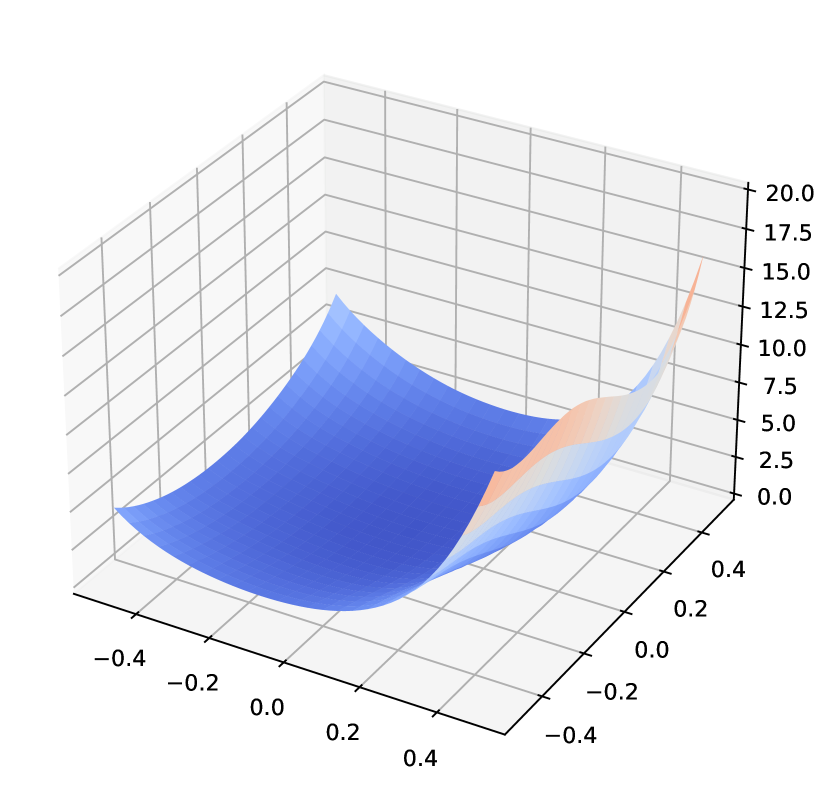
((a)) C-SGD, 128 total batch size

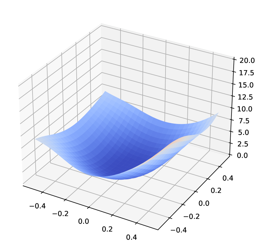
((b)) C-SGD, 1024 total batch size

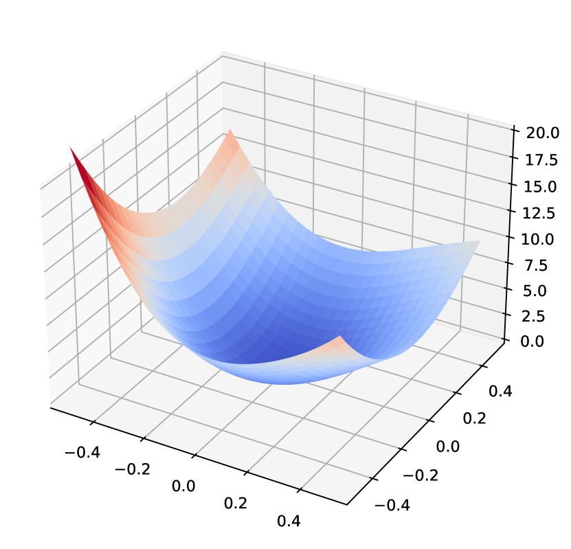
((c)) C-SGD, 8192 total batch size

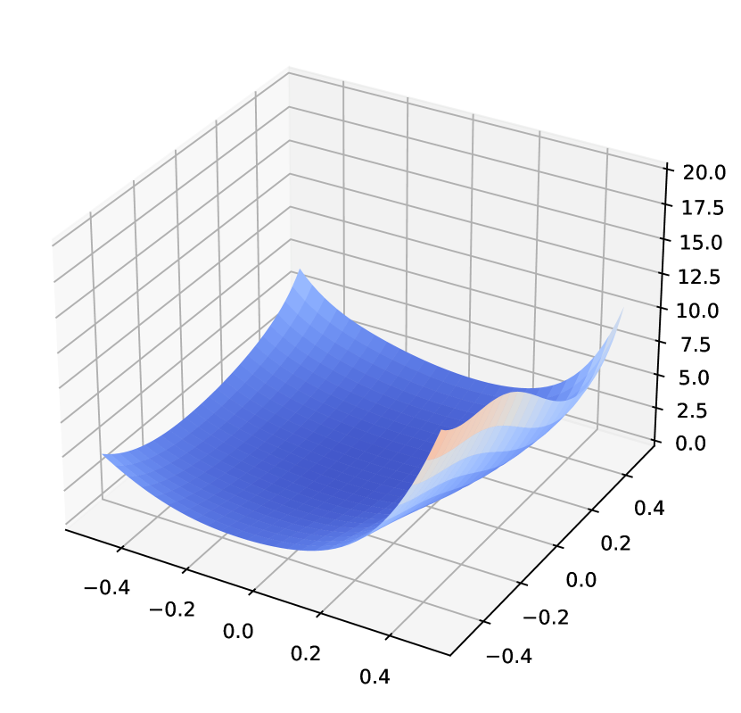
((d)) D-SGD, 128 total batch size

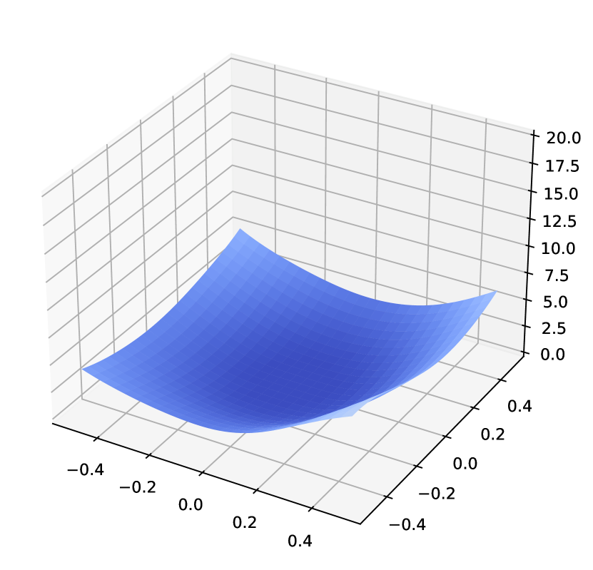
((e)) D-SGD, 1024 total batch size

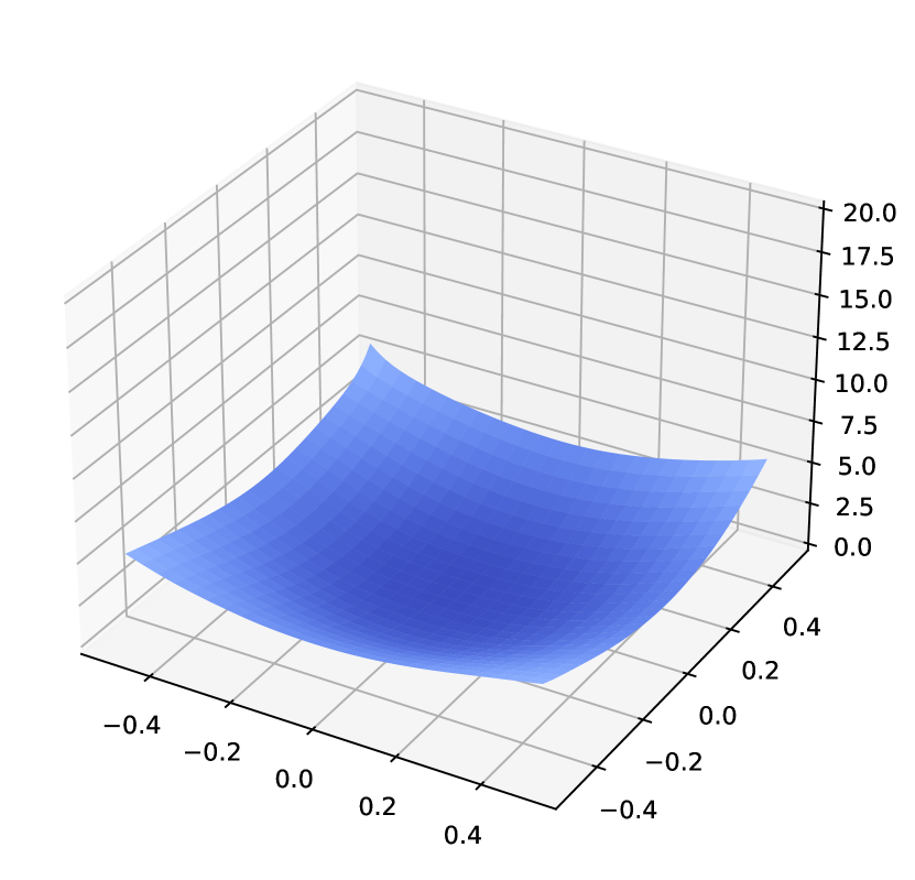
((f)) D-SGD, 8192 total batch size

Figure 3: Minima 3D visualization of ResNet-18 trained on CIFAR-10 using C-SGD and D-SGD (ring topology).

4.4 Generalization benefit of decentralization: the role of total batch size

In practice, data and model decentralization ordinarily imply large total batch sizes, as a massive number of workers are involved in the system in many practical scenarios. Large-batch training can enhance the utilization of super computing facilities and further speed up the entire training process. Thus, studying the large-batch setting is crucial for fully understanding the application of D-SGD.

Despite the importance, theoretical understanding of the generalization of large-batchdecentralized training remains an open problem. This subsection examines the implicit regularization of D-SGD with respect to (w.r.t.) total batch size $|\mu|$, and compares it to C-SGD. To investigate the impact of $|\mu|$, we analyze the effect of the gradient variance, in addition to the gradient expectation studied in Subsection 4.1.

Theorem 3.

Let $B=|\mu|$ denote the total batch size. With a probability greater than $1-\mathcal{O}(\frac{B}{(N-B)\eta^{2}})$, D-SGD implicit minimizes the following objective function:

$${\bm{L}}_{\mathbf{w}}^{\text{\tiny D-SGD}}\scalebox{0.75}[1.0]{$=$}{\bm{L}}_{\mathbf{w}}^{\mu}\scalebox{0.75}[1.0]{$+$}\underbrace{\operatorname{Tr}({\bm{H}}_{\mathbf{w}}^{\mu}\bm{\Xi}{\scriptstyle(t)})\scalebox{0.75}[1.0]{$+$}\frac{\eta}{4}\operatorname{Tr}({({\bm{H}}^{\mu}_{\mathbf{w}})}^{2}\bm{\Xi}{\scriptstyle(t)})}_{\text{batch size independent sharpness regularizer}}$$

$$\scalebox{0.75}[1.0]{$+$}\underbrace{\mathchoice{\leavevmode\hbox to5.76pt{\vbox to4.31pt{\text{[drawing]}}}}{\leavevmode\hbox to5.76pt{\vbox to4.31pt{\text{[drawing]}}}}{\leavevmode\hbox to4.03pt{\vbox to3.01pt{\text{[drawing]}}}}{\leavevmode\hbox to2.88pt{\vbox to2.15pt{\text{[drawing]}}}}\cdot\frac{1}{N}\sum_{j=1}^{N}\left[\|\nabla{\bm{L}}_{\mathbf{w}}^{j}\scalebox{0.75}[1.0]{$-$}\nabla{\bm{L}}_{\mathbf{w}}^{\mu}\|_{2}^{2}\scalebox{0.75}[1.0]{$+$}\operatorname{Tr}({({\bm{H}}_{\mathbf{w}}^{j}\scalebox{0.75}[1.0]{$-$}{\bm{H}}_{\mathbf{w}}^{\mu})}^{2}\bm{\Xi}{\scriptstyle(t)})\right]}_{\text{batch size dependent variance regularizer}} \kappa \kappa$$

$$\scalebox{0.75}[1.0]{$+$}\frac{\eta}{4}\|\nabla{\bm{L}}_{\mathbf{w}}^{\mu}\|_{2}^{2}\scalebox{0.75}[1.0]{$+$}\mathcal{R}^{A}\scalebox{0.75}[1.0]{$+$}\mathcal{O}{(\eta^{2})},$$

where $\kappa=\frac{\eta}{B}\cdot\frac{N\scalebox{0.75}[1.0]{$-$}B}{(N\scalebox{0.75}[1.0]{$-$}1)}$, and $\mathcal{R}^{A}$ absorbs all higher-order residuals. The empirical gradient $\nabla{\bm{L}}^{\mu}_{\mathbf{w}}$ on the super-batch $\mu$ are averaged over the one-sample gradients $\nabla{\bm{L}}_{\mathbf{w}}^{j}\ (j=1,\dots,m)$. Similarly, the empirical Hessian ${\bm{H}}_{\mathbf{w}}^{\mu}$ is an average of ${\bm{H}}_{\mathbf{w}}^{j}={\bm{H}}(\mathbf{w};z_{j})\ (j=1,\dots,m)$.

A corresponding implicit regularization of C-SGD (and SGD) is established in Lemma C.6, which demonstrates that C-SGD has an implicit gradient variance reduction mechanism to improve generalization (see Figure C.1). However, as the total batch size $B$ approaches the total training sample size $N$, the regularization term diminishes rapidly, even in the case when the learning rate scales with the total batch size, since the ratio $\kappa=\frac{N-B}{N-1}$ converges to $0$ gradually.

On the contrary, Theorem 3 proves that the sharpness regularization terms in D-SGD do not decrease as the total batch size increases, unlike in C-SGD, which theoretically justifies the potential superior generalizability of D-SGD in large-batch settings. The underlying intuition is that decentralization introduces additional noise, which compensates for the noise required for D-SGD to generalize well in large-batch scenarios. The proof is included in Subsection C.4.

5 Empirial results

This section empirically validates our theory. We introduce the experimental setup and then study how decentralization impacts minima flatness via local landscape visualization.

Dataset and architecture. Decentralized learning is simulated in a dataset-centric setup by uniformly partitioning data among multiple workers (GPUs) to accelerate the training process. Vanilla D-SGD with various commonly used topologies (see Figure 2) and C-SGD are employed to train image classifiers on CIFAR-10 (Krizhevsky et al., 2009) and Tiny ImageNet (Le & Yang, 2015) with AlexNet (Krizhevsky et al., 2017), ResNet-18 (He et al., 2016b) and DenseNet-121 (Huang et al., 2017). Detailed implementation setting is inclued in Appendix B.

As demonstrated in Figure 1, Figure B.1 and Figure B.2, D-SGD could outperform C-SGD in terms of generalizability in large-batch settings. We also note that the gap in generalizability between D-SGD and C-SGD in a large-batch scenario is larger on the CIFAR-10 dataset, which we attribute to the smaller $\kappa$ value (see Theorem 3). To further support our claim that D-SGD favors flatter minima than C-SGD in large-batch scenarios, we plotted the minima learned by both algorithms using the loss landscape visualization tool in Li et al. (2018). The resulting plots are shown in Figure 3, along with additional plots in Appendix B.

These figures demonstrate that D-SGD could learn flatter minima than C-SGD in large-batch settings, and this difference in flatness becomes larger as the total batch size increases. These observations are consistent with the claims made in Theorem 1 and Theorem 3 that D-SGD favors flatter minima than its centralized counterpart, especially in the large-batch scenarios. Future work includes visualizing the whole trajectories of D-SGD.

6 Discussion and Broader Impact

Question 1: How to scale learning rate w.r.t. batch size and spectral gap in decentralized deep learning?

As proved in Theorem 1, the training dynamics of D-SGD and C-SGD are completely different. There also exists potential landscape smoothing and batch size-independent regularization effect of D-SGD (Corollary 2 and Theorem 3). Consequently, we conjecture that D-SGD could be more “tolerable” to hyperparameters such as learning rate than C-SGD. However, the existing tricks for hyperparameter tuning are tailored for C-SGD (e.g., linear scaling rule). A natural question is that can we design a general scaling strategy of learning rate as a function of batch size and the spectral gap of the communication topology, in order to maintain generalizability of D-SGD in large-batch settings?

Question 2: Would continuously reducing spectral gap improve the validation performance of D-SGD?

The answer is negative, as D-SGD inherently exhibits a regularization-optimization trade-off. On the one hand, a sparse topology with a too-small spectral gap leads to large consensus distance (see proof in Proposition C.1), which also slows down the converges of the higher-order residual terms, and consequently, hampers the optimization of the original objective. On the other hand, although a small spectral gap increases the sharpness regularization effect, it also makes the optimization of $\mathbb{E}_{\epsilon\sim\mathcal{N}(0,\bm{\Xi}{\scriptstyle(t)})}[\nabla{\bm{L}}_{\mathbf{w}_{a}{\scriptstyle(t)}+\epsilon}]$ difficult. In SAM, a too large perturbation radius (or neighborhood size) $\rho$ incurs divergence (Andriushchenko & Flammarion, 2022; Mueller & Hein, 2022). Similarly, a topology with a small spectral gap leads to a large $\operatorname{Tr}{(\bm{\Xi{\scriptscriptstyle(t)}})}$, the magnitude of the variance of $\epsilon$. A large $\operatorname{Tr}{(\bm{\Xi{\scriptscriptstyle(t)}})}$ results in an increased search space for the optimization problem $\min_{\mathbf{w}}\mathbb{E}_{\epsilon\sim\mathcal{N}(0,\bm{\Xi}{\scriptstyle(t)})}[{\bm{L}}_{\mathbf{w}+\epsilon}-{\bm{L}}_{\mathbf{w}}]$, making it more difficult to solve. These intuitions align with the observation that the D-SGD converges slowly on sparse topologies (Lian et al., 2017; Koloskova et al., 2020). Based on the analysis, we conjecture that there exists “sweet spots”, which balance the sharpness regularization introduced by proper decentralization and the optimization issues originated from sparse topologies. Finding these “sweet spots” then becomes a promising direction in a decentralized deep learning.

Future work 1: Fine-grained convergence and generalization analyses of decentralized learning algorithms.

We have demonstrated several potential benefits of D-SGD based on the established equivalence. Another direct extension of our work is to utilize the connection between decentralized learning and centralized learning to improve the existing convergence and generalization bounds of decentralized learning algorithms.

Future work 2: Provide adversarial robustness guarantees for decentralized learning algorithms.

Cao et al. (2023) find that decentralized stochastic gradient algorithms are more adversarial robust than their centralized counterpart in certain scenarios. They boldly conjecture that the superiority could be attributed to their inclination towards flatter minimizers. The question is can we provide rigorous adversarial robustness guarantees of decentralized learning algorithms, and develop more robust algorithms?

Future work 3: Bridge decentralized learning and SAM.

An interesting question arising from the asymptotic equivalence is that does D-SGD share the properties of SAM, beyond generalizablity, including better interpretability (Andriushchenko et al., 2023) and transferability (Chen et al., 2022)? Furthermore, it is worth exploring whether the insights gained from SAM (Andriushchenko & Flammarion, 2022; Möllenhoff & Khan, 2023; Wen et al., 2023) can be utilized to design more effective decentralized algorithms.

7 Conclusion

This paper challenges the conventional belief that centralized learning is optimal in generalizablity and establishes a surprising asymptotic equivalence of decentralized SGD and average-direction SAM. This asymptotic equivalence further demonstrates a regularization-optimization trade-off and three advantages of D-SGD: (1) there exists a surprising free uncertainty estimation mechanism in D-SGD to estimate the intractable posterior covariance; (2) D-SGD has a gradient smoothing effect; and (3) the sharpness regularization effect of D-SGD does not decrease as total batch size increases, which justifies the superior generalizablity of D-SGD over centralized SGD (C-SGD) in large-batch settings. Although our theory focuses primarily on the vanilla decentralized SGD, we believe our theoretical insights are applicable to a broad range of decentralized gradient-based algorithms. Code is available at  D-SGD and SAM.

Appendix A Background

A.1 Distributed centralized training (data decentralization)

Efficiently training large-scale models on massive amounts of data is challenging yet important for real-world applications (Narayanan et al., 2021; Shen et al., 2023). To handle an increasing amount of data and parameters, distributed training on multiple workers emerges. Traditional distributed training systems usually follow a centralized setup (parameter server).

Distributed centralized stochastic gradient descent (C-SGD). In C-SGD (Dean et al., 2012; Li et al., 2014), the de facto distributed training algorithm, there is only one centralized model $\mathbf{w}_{a}{\scriptstyle(t)}$. C-SGD updates the model by

$$\mathbf{w}_{a}{\scriptstyle(t+1)}=\mathbf{w}_{a}{\scriptstyle(t)}-\eta\cdot\frac{1}{m}\sum_{j=1}^{m}\overbrace{\nabla{\bm{L}}^{\mu_{j}{\scriptstyle(t)}}(\mathbf{w}_{a}{\scriptstyle(t)})}^{\text{Local gradient computation}},$$ (A.1)

where $\eta$ is the learning rate, $\mu_{j}{\scriptstyle(t)}=\{z_{j,1},\ldots,z_{j,|\mu_{j}{\scriptstyle(t)}|}\}$ denotes the local training batch independent and identically distributed (i.i.d.) drawn from the data distribution $\mathcal{D}$ at the $t$-th iteration, and $\nabla{\bm{L}}^{\mu_{j}{\scriptstyle(t)}}_{\mathbf{w}}=\nabla{\bm{L}}^{\mu_{j}{\scriptstyle(t)}}(\mathbf{w})=\frac{1}{|\mu_{j}{\scriptstyle(t)}|}\sum_{\zeta{\scriptstyle(t)}=1}^{|\mu_{j}{\scriptstyle(t)}|}\nabla{\bm{L}}({\mathbf{w}};z_{j,\zeta{\scriptstyle(t)}})$ stacks for the local mini-batch gradient of ${\bm{L}}$ w.r.t. the first argument $\mathbf{w}$. The total batch size of C-SGD at $t$-th iteration is $|\mu{\scriptstyle(t)}|=\sum_{j=1}^{m}|\mu_{j}{\scriptstyle(t)}|$.

“Centralized” refers to the fact that in C-SGD, there is a central server receiving weight or gradient information from local workers (see Figure 2). To clarify, the process of updating the global model with the globally averaged gradients, as shown in equation A.1, is equivalent to averaging the local weights after performing local gradient updates on the global model:

$$\mathbf{w}_{j}{\scriptstyle(t+1)}=\mathbf{w}_{j}{\scriptstyle(t)}-\eta\cdot\nabla{\bm{L}}^{\mu_{j}{\scriptstyle(t)}}(\mathbf{w}_{a}{\scriptstyle(t)}),\quad\mathbf{w}_{a}{\scriptstyle(t+1)}=\frac{1}{m}\sum_{j=1}^{m}\mathbf{w}_{j}{\scriptstyle(t+1)},$$

$$\Rightarrow \mathbf{w}_{a}{\scriptstyle(t+1)}=\mathbf{w}_{a}{\scriptstyle(t)}-\eta\cdot\frac{1}{m}\sum_{j=1}^{m}\overbrace{\nabla{\bm{L}}^{\mu_{j}{\scriptstyle(t)}}(\mathbf{w}_{a}{\scriptstyle(t)})}^{\text{Local gradient computation}}.$$ (A.2)

C-SGD defined in Eq. A.1 and Subsection A.1 are mathematically identical to the Federated Averaging algorithm (McMahan et al., 2017) under the condition that the local step is set as $1$ and all local workers are selected by the server in each round. To avoid misunderstandings, we include the term “distributed” in C-SGD to differentiate it from traditional single-worker SGD (Cauchy et al., 1847; Robbins, 1951).

A.2 Decentralized training (data and model decentralization)

Limitations of server-based training. Despite convenience and scalability, central server-based training scheme suffers from two main issues: (1) a centralized communication protocol slows down training since central servers are easily overloaded, especially in low-bandwidth or high-latency cases (Lian et al., 2017); (2) there exists a potential information leakage through privacy attacks on the gradients transmitted to central server despite decentralizing data using Federated Learning (Zhu et al., 2019a; Geiping et al., 2020; Yin et al., 2021; Wang et al., 2023). As an alternative, decentralized learning (machine learning in a peer-to-peer architecture) allows workers to balance the load on the central server (Lian et al., 2017), as well as maintain confidentiality (Warnat-Herresthal et al., 2021).

Development of decentralized algorithms. The earliest work of classical decentralized optimization can be traced back to Tsitsiklis (1984), Tsitsiklis et al. (1986) and Nedic & Ozdaglar (2009). Decentralized SGD, a direct combination of decentralization and gradient-based optimization, has been extended to various contexts, including time-varying topologies (Nedić & Olshevsky, 2014; Lu & Wu, 2020; Koloskova et al., 2020; Ying et al., 2021a), directed topologies (Assran et al., 2019; Taheri et al., 2020; Song et al., 2022), asynchronous settings (Lian et al., 2018; Xu et al., 2021; Nadiradze et al., 2021; Bornstein et al., 2023), personalized settings (Li et al., 2022; Shi et al., 2023a), data-heterogeneous scenarios (Tang et al., 2018; Vogels et al., 2021; Le Bars et al., 2023; Shi et al., 2023b) and Byzantine-robust versions (Yang et al., 2020; Farhadkhani et al., 2023). Although our theory focuses primarily on the vanilla decentralized SGD, we anticipate our theoretical insights will be applicable to a broad range of decentralized algorithms.

We then summarize some commonly used notions regarding decentralized training in the following.

Definition A.1 (Doubly Stochastic Matrix).

Let $\mathcal{G}=(\mathcal{V},\mathcal{E})$ stand for the decentralized communication topology, where $\mathcal{V}$ denotes the set of $m$ computational nodes and $\mathcal{E}$ represents the edge set. For any given topology $\mathcal{G}=(\mathcal{V},\mathcal{E})$, the doubly stochastic gossip matrix ${\mathbf{P}}=[\mathbf{P}_{j,k}]\in\mathbb{R}^{m\times m}$ is defined on the edge set $\mathcal{E}$ that satisfies

• ${\mathbf{P}}={\mathbf{P}}^{\top}$ (symmetric);

• If $j\neq k$ and $(j,k)\notin{\cal E}$, then $\mathbf{P}_{j,k}=0$ (disconnected) and otherwise, $\mathbf{P}_{j,k}>0$ (connected);

• $\mathbf{P}_{j,k}\in[0,1]\ \ \forall k,l$ and $\sum_{k}\mathbf{P}_{j,k}=\sum_{l}\mathbf{P}_{j,k}=1$ (standard weight matrix for undirected graph).

The doubly stochasticity of the gossip matrices is a standard assumption in decentralized learning (Lian et al., 2017; Koloskova et al., 2020). It is worth noticing that our theory is generally applicable to arbitrary communication topologies whose gossip matrices are doubly stochastic.

In the following we illustrate some commonly-used communication topologies.

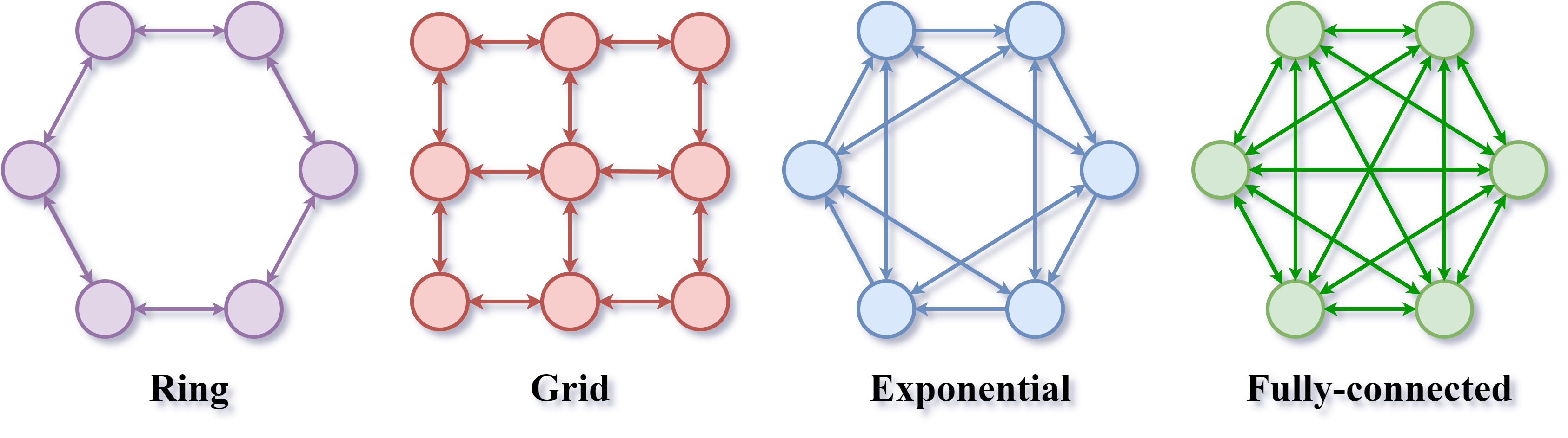
Figure A.1: An illustration of some commonly used topologies.

The intensity of gossip communications is measured by the spectral gap (Seneta, 2006) of $\mathbf{P}$.

Definition A.2 (Spectral Gap).

Denote $\lambda=\max\left\{\left|\lambda_{2}\right|,\left|\lambda_{m}\right|\right\}$ where $\lambda_{i}\ (i=2,\dots,m)$ is the $i$-th largest eigenvalue of gossip matrix ${\mathbf{P}}\in\mathbb{R}^{m\times m}$. The spectral gap of a gossip matrix $\mathbf{P}$ can be defined as follows:

$${\textnormal{spectral gap}}:=1-\lambda.$$

According to the definition of doubly stochastic matrix (Definition A.1), we have $0\leq\lambda<1$. The spectral gap measures the connectivity of the communication topology. A topology is considered sparse if its communication matrix has a small spectral gap close to $0$, while a topology is considered dense if its communication matrix has a large spectral gap close to $1$.

A.3 Sharpness-aware minimization

Sharpness-aware minimization (SAM) is proposed by Foret et al. (2021) to minimize a perturbed loss function for the purpose of improving generalization, which is studied concurrently by Wu et al. (2020) and Zheng et al. (2021). Subsequently, various SAM variants emerge, including adaptive SAM (Kwon et al., 2021), surrogate gap guided SAM (Zhuang et al., 2022), LookSAM (Liu et al., 2022a), Fisher SAM (Kim et al., 2022), random SAM (Liu et al., 2022b), sparse SAM (Mi et al., 2022), variational SAM (Ujváry et al., 2022) and Bayes SAM (Möllenhoff & Khan, 2023).

Definition A.3 (Vanilla SAM (Foret et al., 2021)).

The loss function of vanilla SAM is defined as follows:

$${\bm{L}}^{\text{\tiny SAM}}(\mathbf{w})=\max_{\|\in\|_{p}\leq\rho}{\bm{L}}(\mathbf{w}+\epsilon).$$

Foret et al. (2021) propose to use a first-order approximation to simplify the max step:

$${\bm{L}}^{\text{\tiny SAM}}(\mathbf{w})\approx\max_{\|\in\|_{p}\leq\rho}[{\bm{L}}(\mathbf{w})+\epsilon^{\top}\nabla{\bm{L}}(\mathbf{w})],$$

where $\epsilon^{*}=\rho\frac{\nabla{\bm{L}}(\mathbf{w})}{\|\nabla{\bm{L}}(\mathbf{w})\|_{2}}$ is the close-form solution.

Therefore, the gradient update of vanilla SAM becomes

$$\nabla{\bm{L}}^{\text{\tiny SAM}}(\mathbf{w})\approx\nabla{\bm{L}}(\mathbf{w}+\epsilon^{*})=\nabla{\bm{L}}(\mathbf{w}+\rho\frac{\nabla{\bm{L}}(\mathbf{w})}{\|\nabla{\bm{L}}(\mathbf{w})\|_{2}}).$$

Definition A.4 (Average-direction SAM (Wen et al., 2023)).

Average-direction SAM (AD-SAM) minimizes

$${\bm{L}}^{\text{\tiny AD-SAM}}(\mathbf{w})=\mathbb{E}_{\epsilon\sim\mathcal{N}(0,I)}[{\bm{L}}({\mathbf{w}+\epsilon^{\top}\frac{\nabla{\bm{L}}(\mathbf{w})}{\|\nabla{\bm{L}}(\mathbf{w})\|_{2}}})].$$

Average-direction is named because it minimizes an averaged loss in a “basin” around $\mathbf{w}$, rather than the original point-loss. Actually, the generalization bound of vanilla SAM in Foret et al. (2021) upper bounds the generalization error by the average-direction sharpness ${\bm{L}}^{\text{\tiny AD-SAM}}(\mathbf{w})-{\bm{L}}(\mathbf{w})$. However, Wen et al. (2023) proves that average-direction SAM actually minimizes ${\bm{L}}(\mathbf{w})+\operatorname{Tr}({{\bm{H}}(\mathbf{w})})$ rather than $\max_{\|\in\|_{p}\leq\rho}{\bm{L}}(\mathbf{w}+\epsilon)$.

The average-direction SAM that defined in our paper is sightly different from that in (Wen et al., 2023):

$${\underbrace{{\mathchoice{\leavevmode\hbox to73.67pt{\vbox to11pt{\text{[drawing]}}}}{\leavevmode\hbox to73.67pt{\vbox to11pt{\text{[drawing]}}}}{\leavevmode\hbox to54.03pt{\vbox to8.75pt{\text{[drawing]}}}}{\leavevmode\hbox to48.17pt{\vbox to7.25pt{\text{[drawing]}}}}}}_{\text{{average-direction sharpness}}}}. \mathbb{E}_{\epsilon\sim\mathcal{N}(0,\bm{\Xi}{\scriptstyle(t)})}[{\bm{L}}_{\mathbf{w}+\epsilon}-{\bm{L}}_{\mathbf{w}}] \mathbb{E}_{\epsilon\sim\mathcal{N}(0,\bm{\Xi}{\scriptstyle(t)})}[{\bm{L}}_{\mathbf{w}+\epsilon}-{\bm{L}}_{\mathbf{w}}]$$

This kind of AD-SAM depends both on the local landscape and consensus, which is discussed in detail in Subsection 4.1.

A.4 Generalization in large-batch training

Large-batch training is of significant interest for deep learning deployment, which can contribute to a significant speed-up in training neural networks (Goyal et al., 2017; You et al., 2018; Shallue et al., 2019). Unfortunately, it is widely observed that in the centralized learning setting, large-batch training often suffers from a drastic generalization degradation, even with fine-tuned hyperparameters, from both empirical (Chen & Huo, 2016; Keskar et al., 2017; Hoffer et al., 2017; Shallue et al., 2019; Smith et al., 2020, 2021) and theoretical (He et al., 2019; Li et al., 2021) aspects. An explanation of this phenomenon is that large-batch training lacks sufficient gradient noise to escape “sharp” minima (Smith et al., 2020).

Mitigating generalization issues in large-batch training. Linear scaling rule (LSR) is a widely used hyper-parameter-free rule to make up the noise in large-batch deep learning (He et al., 2016a; Goyal et al., 2017; Bottou et al., 2018; Smith et al., 2020), which states that a fixed learning rate to total batch size ratio allows maintaining generalization performance when the total batch size increases. Apart from LSR, various optimization techniques have been proposed to reduce the gap, including learning rate warmup (Smith, 2017), Layer-wise Adaptive Rate Scaling (LARS) (You et al., 2017) and Layer-wise Adaptive Moments (LAMB) (You et al., 2020). Is worth noticing that decentralization could be a general training technique in a data-centric setup, which can be combined with these approaches to further improve generalization in large-batch training.

A.5 $\beta$-smoothness

Smoothness is a fundamental property of the objective function in optimization, which characterizes the behavior of its gradient with respect to changes in the parameters (Boyd et al., 2004). In particular, $\beta$-smoothness quantifies the rate at which the objective function varies with respect to changes in the input variables, which is demonstrated as follow:

Definition A.5 ($\beta$-smoothness).

${\bm{L}}$ is $\beta$-smooth if for any $z$ and $\mathbf{w},\widetilde{\mathbf{w}}\in\mathbb{R}^{d}$,

$$\big{\|}\nabla{\bm{L}}(\mathbf{w};z)-\nabla{\bm{L}}(\widetilde{\mathbf{w}};z)\big{\|}_{2}\leq\beta\|\mathbf{w}-\widetilde{\mathbf{w}}\|_{2}.$$ (A.3)

An objective function that lacks $\beta$-smoothness (i.e., non-$\beta$-smoothness) can exhibit sudden variations in its gradient with respect to the input variables, making it difficult to predict the behavior of the function and to design efficient optimization algorithms. However, $\beta$-smoothness is generally difficult to ensure at the beginning and intermediate phases of deep neural network training (Bassily et al., 2020). It is noteworthy that our theoretical framework does not rely on the $\beta$-smoothness assumption of the objective function ${\bm{L}}$, which renders it suited for different stages of deep neural network training.

A.6 Explanation of tensor product

The tensor product between a third-order tensor ${\bm{T}}\in\mathbb{R}^{d\times d\times d}$ and a second-order tensor (matrix) ${\bm{M}}\in\mathbb{R}^{d\times d}$ in the proof of Theorem 1 is defined as

$$\underbrace{{({\bm{T}}\otimes{\bm{M}})}_{i}}_{\text{the $i$-th entry}}=\text{grandsum}{({\bm{T}}_{i}\odot{\bm{M}})},$$

where ${\bm{T}}_{i}\in\mathbb{R}^{d\times d}$ is a second-order tensor (matrix), $\odot$ denotes the Hadamard product (Davis, 1962), and the $\text{grandsum}(\cdot)$ (Merikoski, 1984) of a second-order tensor (matrix) $\tilde{{\bm{M}}}$ satisfies $\text{grandsum}(\tilde{{\bm{M}}})=\sum_{i,j}\tilde{{\bm{M}}}_{ij}$.

Appendix B Experimental Setup and Additional Results

This section provides a comprehensive account of the experimental setup, along with supplementary experiments comparing the generalization performance and the sharpness of the minima of C-SGD and D-SGD. The validation accuracy comparison of C-SGD and D-SGD includes three scenarios: on multiple communication topologies, without pretraining, and using layer-wise learning rate tuning.

Dataset and architecture. Decentralized learning is simulated in a dataset-centric setup by uniformly partitioning data among multiple workers (GPUs) to accelerate training. Vanilla D-SGD with various commonly used topologies (see Figure 2) and C-SGD are employed to train image classifiers on CIFAR-10 (Krizhevsky et al., 2009) and Tiny ImageNet (Le & Yang, 2015) with AlexNet (Krizhevsky et al., 2017), ResNet-18 (He et al., 2016b) and DenseNet-121 (Huang et al., 2017). The ImageNet pretrained models are used as initializations to achieve better final validation performance.

Implementation setting. The number of workers (one GPU as a worker) is set as 16; and the local batch size is set as 8, 64, and 512 per worker in different cases. For the case of local batch size 64, the initial learning rate is set as $0.1$ for ResNet-18 and ResNet-34 and $0.01$ for AlexNet, following the setup in (Zhang et al., 2021). The learning rate is divided by $10$ when the model has passed the $2/5$ and $4/5$ of the total number of iterations (He et al., 2016a). We apply the learning rate warm-up (Smith, 2017) and the linear scaling law (He et al., 2016a; Goyal et al., 2017) to maintain generalization performance with increased total batch size. Batch normalization (Ioffe & Szegedy, 2015) is employed in training AlexNet. In order to understand the effect of decentralization on the flatness of minima and generalization, all other training techniques are strictly controlled. The training accuracy is almost $100\%$ everywhere. Exponential moving average is employed to smooth the validation accuracy curves in Figure 1, Figure B.1 and Figure B.2. The code is based on PyTorch (Paszke et al., 2019).

Hardware environment. The experiments are conducted on a computing facility with NVIDIA^® Tesla^™ V100 16GB GPUs and Intel^® Xeon^® Gold 6140 CPU @ 2.30GHz CPUs.

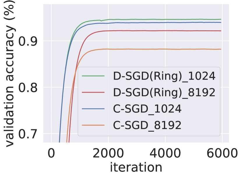
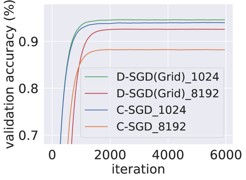
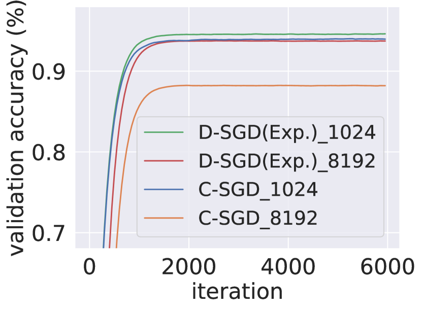
Figure B.1: The validation accuracy comparison of ResNet-18 trained on CIFAR-10 using C-SGD and D-SGD with various topologies (see Figure 2). The number of workers (one GPU as a worker) is set as 16; and the local batch size is set as 64, and 512 per worker (1024 and 8196 total batch size).

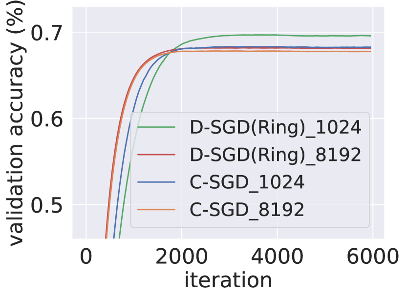
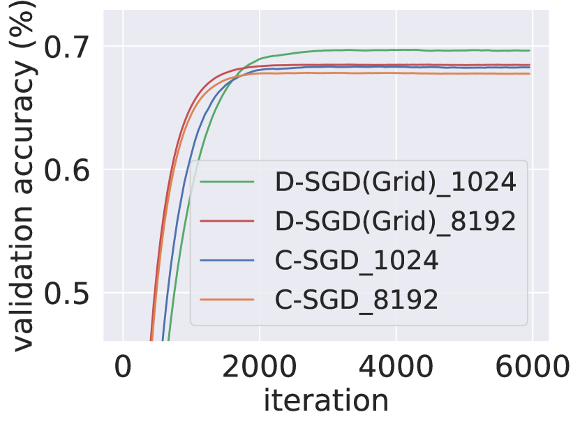
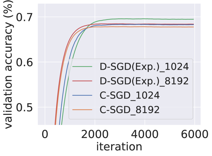
Figure B.2: The validation accuracy comparison of ResNet-18 trained on Tiny ImageNet using C-SGD and D-SGD with various topologies (see Figure 2). The number of workers (one GPU as a worker) is set as 16; and the local batch size is set as 64, and 512 per worker.

Figure B.1 and Figure B.2 show that D-SGD with different topologies could outperform C-SGD by a large margin in large-batch settings, which are consistent with the results shown in Figure 1.

Additional experiments without pretraining. Additional experiments are conducted to further investigate the impact of pretraining. All other training settings are kept the same as the previous experiments.

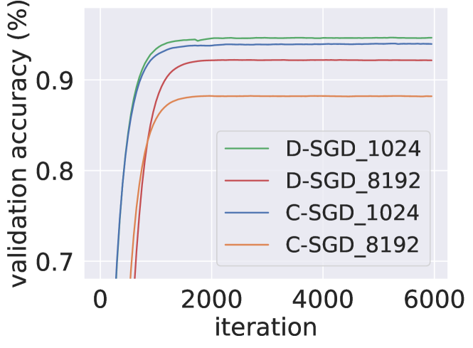
((a)) ResNet-18 (with ImageNet pretrained weights)

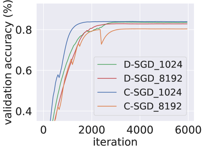
((b)) ResNet-18 (training from scratch)

Figure B.3: The validation accuracy comparison of ResNet-18 with (left) and without pretraining (right) trained on CIFAR-10 using C-SGD and D-SGD. The number of workers (one GPU as a worker) is set as 16; and the local batch size is set as 64, and 512 per worker.

One can observe from Figure B.3 that the gap in validation accuracy between C-SGD and D-SGD is alleviated in the training-from-scratch settings, which we attributes to the initial optimization difficulties of decentralized training without pretrained weights (see the discussion in Section 6). The findings align with our insight that the generalization benefits of decentralization are more pronounced when optimization is not a significant obstacle. We also note that without pretraining, the accuracy curves of D-SGD are notably smoother than that of C-SGD, which supports the theoretical results in Corollary 2.

Additional experiments on LAMB. Large-batch training is of significant interest for deep learning deployment. However, linearly scaling the learning rate with the batch size can lead to generalization degradation (Shallue et al., 2019; Smith et al., 2020, 2021; Li et al., 2021). To address this issue, specialized methods have been developed to carefully tune the scaling factor between the learning rate and batch size, such as Layer-wise Adaptive Rate Scaling (LARS) (You et al., 2017) and Layer-wise Adaptive Moments (LAMB) (You et al., 2020). LARS calculates a scaling factor based on the ratio of the norm of the weight matrix to the norm of the weight gradients for each layer, while LAMB incorporates adaptive moment estimation. These methods have been shown to improve the convergence rate and generalization performance of large-batch training. We compare the validation accuracy of centralized LAMB (C-LAMB) and decentralized LAMB (D-LAMB). We follow the baseline learning rate setups (i.e., 0.0035 and 0.01) in You et al. (2020) and conduct experiments with other different learning rates, which is shown below.

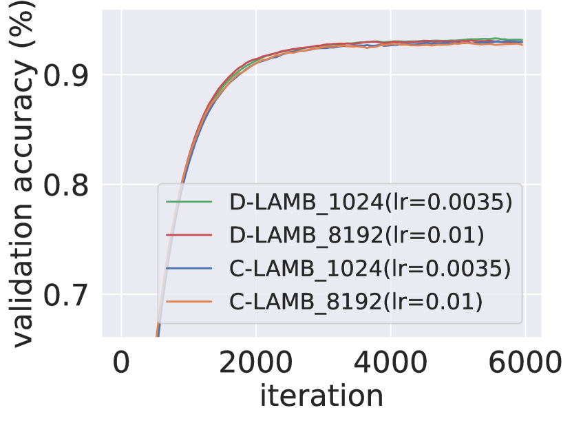
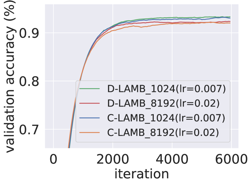
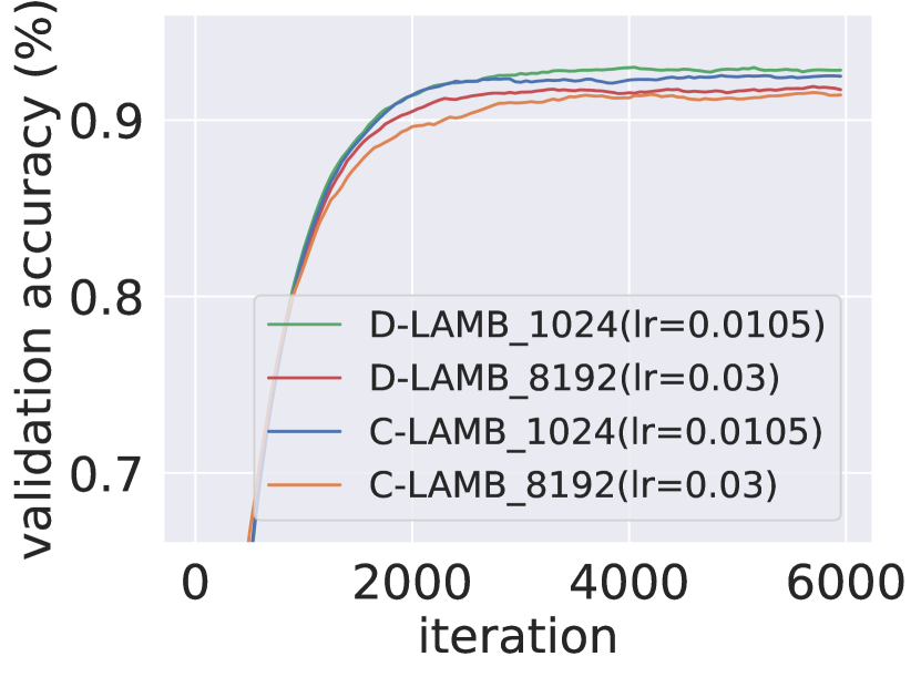
Figure B.4: The validation accuracy comparison of ResNet-18 trained on CIFAR-10 using centralized LAMB (C-LAMB) and decentralized LAMB (D-LAMB, ring topology) with different learning rates. The number of workers (one GPU as a worker) is set as 16; and the local batch size is set as 512 per worker (8196 total batch size). The baseline learning rate setups (i.e., 0.0035 and 0.01) follow You et al. (2020).

The best validation accuracy of C-LAMB training ResNet-18 on CIFAR-10 is 93.06 and 92.03 for 1024 and 8192 total batch size settings, respectively. The best validation accuracy of D-LAMB training ResNet-18 on CIFAR-10 is 93.32 and 92.95 for 1024 and 8192 total batch size settings, respectively. We find LAMB can mitigate the gap in generalizability between centralized training and decentralized training. However, decentralization still offers sight performance benefit on LAMB optimizer on multiple learning rates. Is is worth noticing that compared with LARS and LAMB, decentralization incurs zero additional computation overhead (e.g., no expensive computation of weight norm and gradient norm).

Minima visualizations. The following figures depicts the local loss landscape round minima learned by C-SGD and D-SGD.

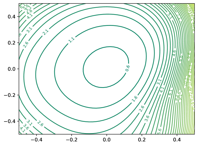
((a)) C-SGD, 128 total batch size

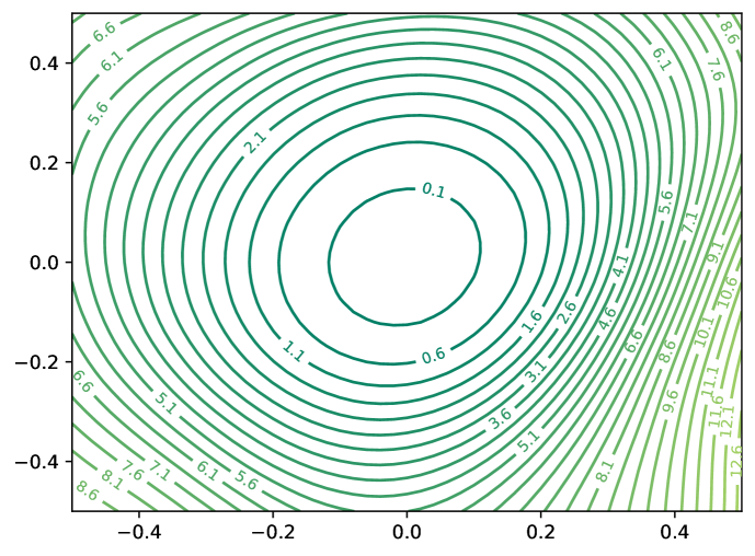
((b)) C-SGD, 1024 total batch size

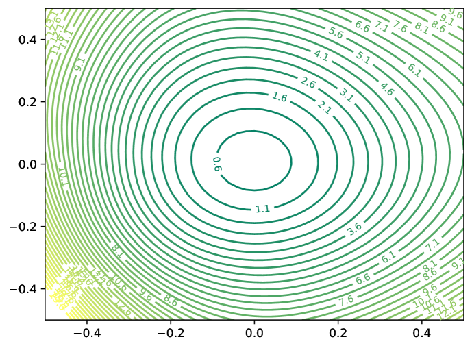
((c)) C-SGD, 8196 total batch size

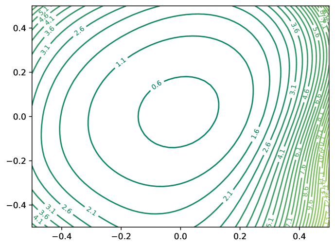
((d)) D-SGD, 128 total batch size

((e)) D-SGD, 1024 total batch size

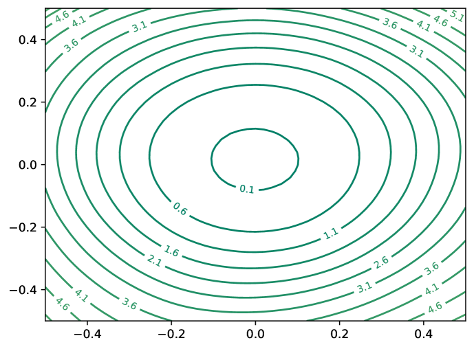
((f)) D-SGD, 8196 total batch size

Figure B.5: Minima 2D visualization of ResNet-18 trained on CIFAR-10 using C-SGD and D-SGD (Ring).

We also compare the minima learned by C-SGD and D-SGD with multiple topologies in Figure B.6.

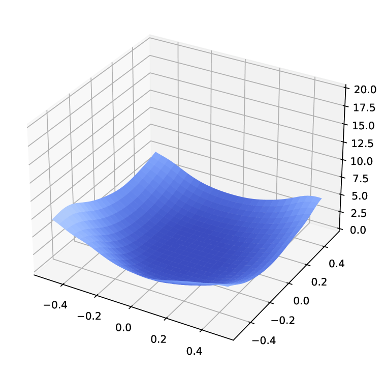
((a)) D-SGD (Ring),
1024 total batch size

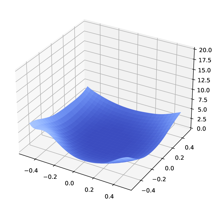
((b)) D-SGD (Grid),
1024 total batch size

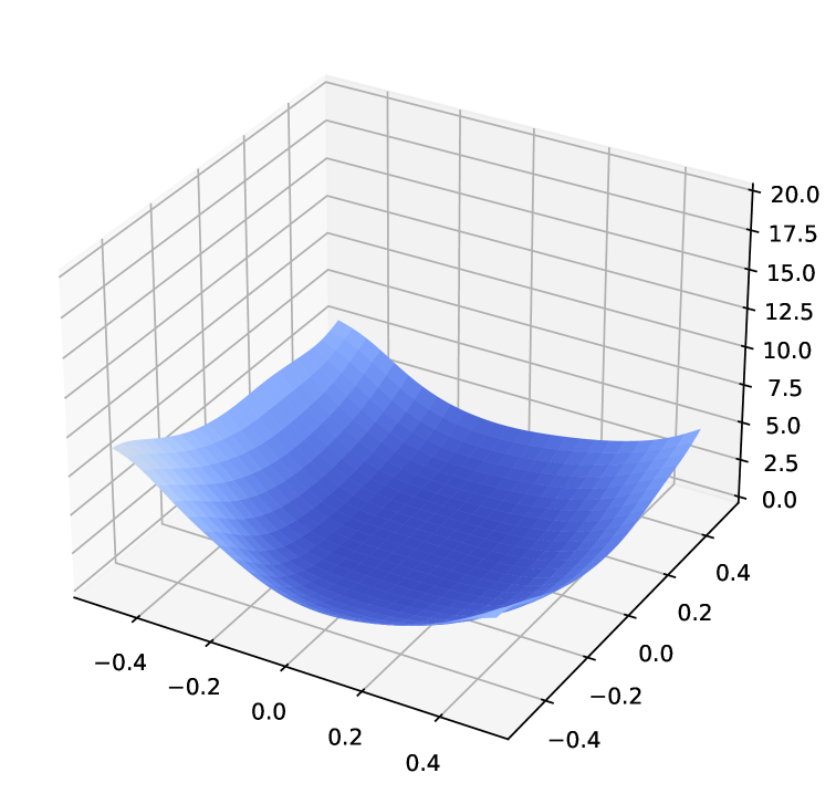
((c)) D-SGD (Exponential),
1024 total batch size

((d)) C-SGD,
1024 total batch size

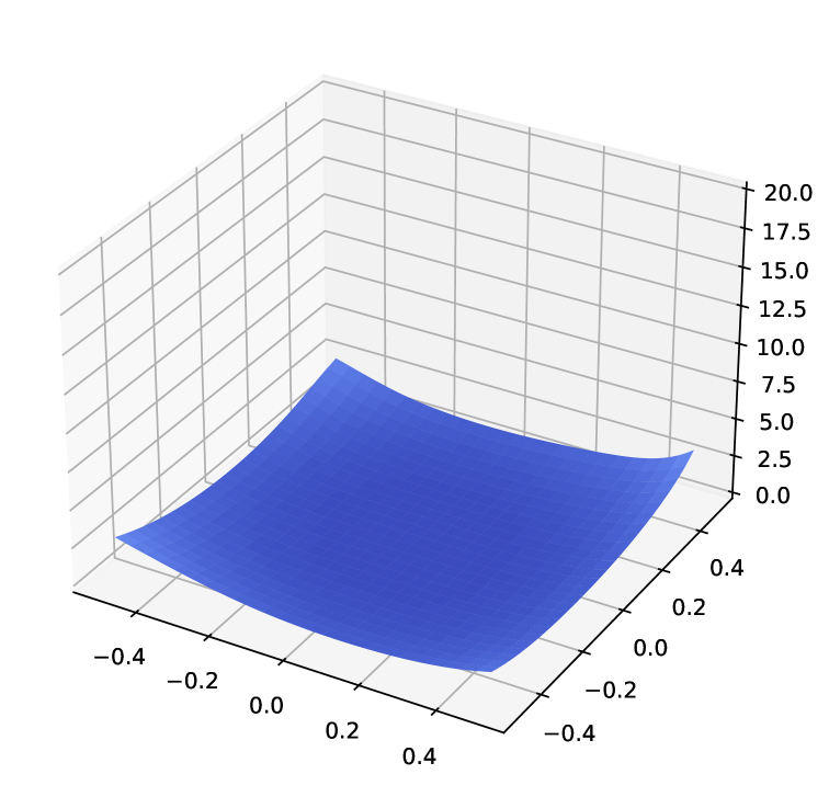
((e)) D-SGD (Ring),
8192 total batch size

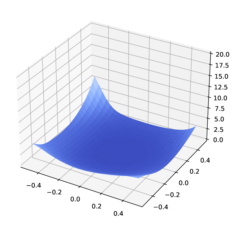
((f)) D-SGD (Grid),
8192 total batch size

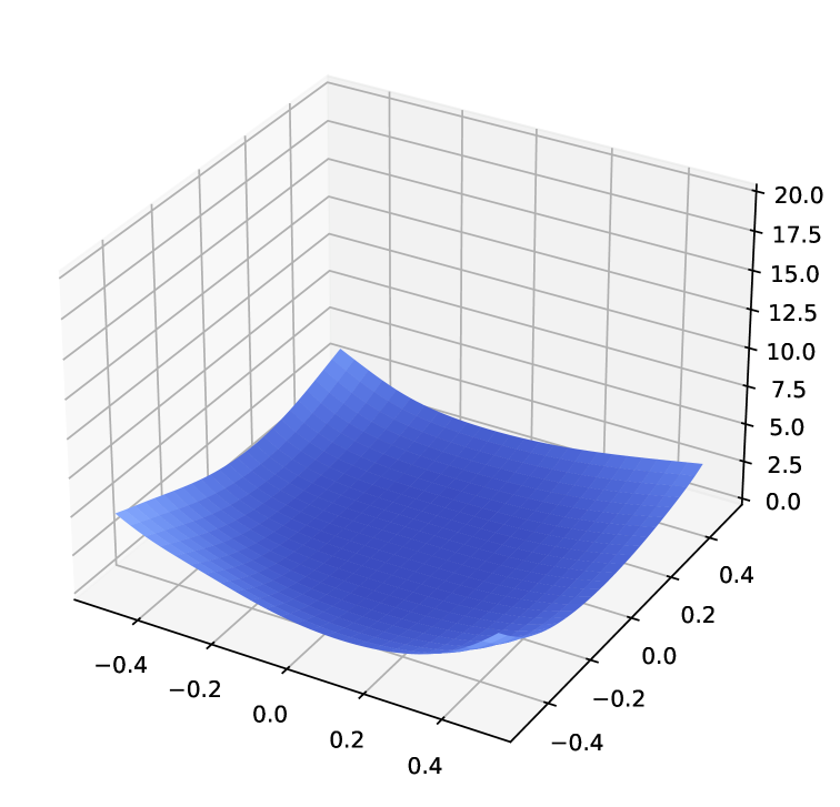
((g)) D-SGD (Exponential),
8196 total batch size

((h)) C-SGD,
8196 total batch size

Figure B.6: Minima 3D visualization of ResNet-18 trained on CIFAR-10 using D-SGD with ring, grid-like and exponential topologies.

From Figure B.5 and Figure B.6, one can observe that (1) the minima of D-SGD with multiple commonly-used topologies could be flatter than those of C-SGD; and that (2) the gap in flatness increases as the total batch size increases. The findings support the claims made by Theorem 1 and Theorem 3.

Appendix C Proof

C.1 Propositions on the consensus distance

We will introduce some useful propositions about the consensus distance, as shown below.

As the terms in brackets are of order $\mathcal{O}{\left(\frac{{(1-\lambda)}^{2}}{{\lambda}}\cdot{\operatorname{Tr}(\bm{\Xi}{\scriptstyle(t)})}\right)}$ according to Proposition C.1, the assumption on $\eta$ becomes $\eta\leq\mathcal{O}{({{\operatorname{Tr}(\bm{\Xi}{\scriptstyle(t)})}}^{\frac{1}{2}})}$. The proof follows directly from Lemma C.2 in (Kong et al., 2021).

The inequality is derived from the generalized mean inequality (Marshall et al., 1979).

C.2 Proof of Theorem 1

Proof of Proposition C.4.

On quadratic loss, we have

$$\frac{1}{m}\sum_{j=1}^{m}[\nabla{\bm{L}}^{\mu_{j}{\scriptscriptstyle(t)}}\left(\mathbf{w}_{j}{\scriptstyle(t)}\right)\scalebox{0.75}[1.0]{$-$}\nabla{\bm{L}}^{\mu_{j}{\scriptscriptstyle(t)}}\left(\mathbf{w}_{a}{\scriptstyle(t)}\right)]=\frac{1}{m}\sum_{j=1}^{m}[{\bm{H}}\mathbf{w}_{j}{\scriptstyle(t)}\scalebox{0.75}[1.0]{$+$}A\scalebox{0.75}[1.0]{$-$}{\bm{H}}\mathbf{w}_{a}{\scriptstyle(t)}\scalebox{0.75}[1.0]{$-$}A]={\bm{H}}\frac{1}{m}\sum_{j=1}^{m}[\mathbf{w}_{j}{\scriptstyle(t)}\scalebox{0.75}[1.0]{$-$}\mathbf{w}_{a}{\scriptstyle(t)}]=0.$$

In distributed centralized SGD, the gradient diversity satisfies

$$\frac{1}{m}\sum_{j=1}^{m}[\nabla{\bm{L}}^{\mu_{j}{\scriptscriptstyle(t)}}\underbrace{\left(\mathbf{w}_{j}{\scriptstyle(t)}\right)}_{=\mathbf{w}_{a}{\scriptstyle(t)}}\scalebox{0.75}[1.0]{$-$}\nabla{\bm{L}}^{\mu_{j}{\scriptscriptstyle(t)}}\left(\mathbf{w}_{a}{\scriptstyle(t)}\right)]=0.$$

∎

It can be deduced directly from Proposition C.4 that distributed centralized SGD, which has constant zero gradient diversity, is equivalent to standard single-worker mini-batch SGD with equivalently large batch size.

Proof of Theorem 1.

(1) Derive the iterate of the averaged model $\mathbf{w}_{a}{\scriptstyle(t)}$.

Directly analyzing the dynamics of the diffusion-like decentralized systems where information is gradually spread across the network is non-trivial. Instead, we focus on $\mathbf{w}_{a}{\scriptstyle(t)}=\frac{1}{m}\sum_{j=1}^{m}\mathbf{w}_{j}{\scriptstyle(t)}$, the global averaged model of D-SGD, whose update can be written as follows,

$$\mathbf{w}_{a}{\scriptstyle(t+1)}\scalebox{0.75}[1.0]{$=$}\mathbf{w}_{a}{\scriptstyle(t)}\scalebox{0.75}[1.0]{$-$}\eta\big{[}\nabla{\bm{L}}^{\mu{\scriptscriptstyle(t)}}_{\mathbf{w}_{a}{\scriptstyle(t)}}\scalebox{0.75}[1.0]{$+$}\underbrace{\frac{1}{m}\sum_{j=1}^{m}(\nabla{\bm{L}}^{\mu_{j}{\scriptscriptstyle(t)}}_{\mathbf{w}_{j}{\scriptstyle(t)}}\scalebox{0.75}[1.0]{$-$}\nabla{\bm{L}}^{\mu_{j}{\scriptscriptstyle(t)}}_{\mathbf{w}_{a}{\scriptstyle(t)}})}_{\text{{gradient diversity among local workers}}}\big{]}.$$ (C.1)

Remark. Eq. C.1 shows that decentralization introduces an additional noise, which characterizes the gradient diversity between the global averaged model $\mathbf{w}_{a}{\scriptstyle(t)}$ and the local models $\mathbf{w}_{j}{\scriptstyle(t)}$ for $j\scalebox{0.75}[1.0]{$=$}1,\dots,m$, compared with its centralized counterpart. Therefore, we note that

analyzing the gradient diversity is the major challenge of decentralized (gradient-based) learning

.

Insight. We also note that the gradient diversity equals to zero on quadratic objective ${\bm{L}}$ (see Proposition C.4). Therefore, the quadratic approximation of loss functions ${\bm{L}}$ (Zhu et al., 2019b; Ibayashi & Imaizumi, 2021; Liu et al., 2021, 2022c) might be insufficient to characterize how decentralization impacts the training dynamics of D-SGD, especially on neural network loss landscapes where quadratic approximation may not be accurate even around minima (Ma et al., 2022). To better understand the dynamics of D-SGD on complex landscapes, it is crucial to consider higher-order geometric information of objective ${\bm{L}}$. In the following, we approximate the gradient diversity using Taylor expansion, instead of analyzing it on non-convex non-$\beta$-smooth loss ${\bm{L}}$ directly, which is highly non-trivial.

(2) Perform Taylor expansion on the gradient diversity. Technically, we perform a second-order Taylor expansion on the gradient diversity around $\mathbf{w}_{a}{\scriptstyle(t)}$:

$$\frac{1}{m} \sum_{j=1}^{m}(\nabla{\bm{L}}^{\mu_{j}{\scriptscriptstyle(t)}}_{\mathbf{w}_{j}{\scriptstyle(t)}}\scalebox{0.75}[1.0]{$-$}\nabla{\bm{L}}^{\mu_{j}{\scriptscriptstyle(t)}}_{\mathbf{w}_{a}{\scriptstyle(t)}})=\frac{1}{m}\sum_{j=1}^{m}{\bm{H}}^{\mu_{j}{\scriptscriptstyle(t)}}_{\mathbf{w}_{a}{\scriptstyle(t)}}\cdot(\mathbf{w}_{j}{\scriptstyle(t)}\scalebox{0.75}[1.0]{$-$}\mathbf{w}_{a}{\scriptstyle(t)})\scalebox{0.75}[1.0]{$+$}\frac{1}{2m}\sum_{j=1}^{m}{\bm{T}}^{\mu_{j}{\scriptscriptstyle(t)}}_{\mathbf{w}_{a}{\scriptstyle(t)}}\otimes[(\mathbf{w}_{j}{\scriptstyle(t)}\scalebox{0.75}[1.0]{$-$}\mathbf{w}_{a}{\scriptstyle(t)})(\mathbf{w}_{j}{\scriptstyle(t)}\scalebox{0.75}[1.0]{$-$}\mathbf{w}_{a}{\scriptstyle(t)})^{\top}],$$

plus residual terms $\mathcal{O}(\frac{1}{m}\sum_{j=1}^{m}\|\mathbf{w}_{j}{\scriptstyle(t)}\scalebox{0.75}[1.0]{$-$}\mathbf{w}_{a}{\scriptstyle(t)}\|_{2}^{3})$. Here ${\bm{H}}^{\mu_{j}{\scriptscriptstyle(t)}}_{\mathbf{w}_{a}{\scriptstyle(t)}}\triangleq\frac{1}{|\mu_{j}{\scriptstyle(t)}|}\sum_{\zeta{\scriptstyle(t)}=1}^{|\mu_{j}{\scriptstyle(t)}|}{\bm{H}}({\mathbf{w}_{a}{\scriptstyle(t)}};z_{j,\zeta{\scriptstyle(t)}})$ denotes the empirical Hessian matrix evaluated at $\mathbf{w}_{a}{\scriptstyle(t)}$ and ${\bm{T}}^{\mu_{j}{\scriptscriptstyle(t)}}_{\mathbf{w}_{a}{\scriptstyle(t)}}\triangleq\frac{1}{|\mu_{j}{\scriptstyle(t)}|}\sum_{\zeta{\scriptstyle(t)}=1}^{|\mu_{j}{\scriptstyle(t)}|}{\bm{T}}({\mathbf{w}_{a}{\scriptstyle(t)}};z_{j,\zeta{\scriptstyle(t)}})$ stacks for the empirical third-order partial derivative tensor at $\mathbf{w}_{a}{\scriptstyle(t)}$, where $\mu_{j}{\scriptstyle(t)}$ and $z_{j,\zeta{\scriptstyle(t)}}$ follows the notation in Eq. 1.

As $\mathbf{w}_{a}{\scriptstyle(t)}$ and local models $\mathbf{w}_{j}{\scriptstyle(t)}\ (j\scalebox{0.75}[1.0]{$=$}1,\dots,m)$ are only correlated with the super batch before the $t$-th iteration (see Eq. 2), taking expectation over $\mu{\scriptscriptstyle(t)}$ provides

$$\mathbb{E}_{\mu{\scriptscriptstyle(t)}} \big{[}\frac{1}{m}\sum_{j=1}^{m}(\nabla{\bm{L}}^{\mu_{j}{\scriptscriptstyle(t)}}_{\mathbf{w}_{j}{\scriptstyle(t)}}\scalebox{0.75}[1.0]{$-$}\nabla{\bm{L}}^{\mu_{j}{\scriptscriptstyle(t)}}_{\mathbf{w}_{a}{\scriptstyle(t)}})\big{]}={\bm{H}}_{\mathbf{w}_{a}{\scriptstyle(t)}}\cdot\underbrace{\frac{1}{m}\sum_{j=1}^{m}(\mathbf{w}_{j}{\scriptstyle(t)}\scalebox{0.75}[1.0]{$-$}\mathbf{w}_{a}{\scriptstyle(t)})}_{=0}\scalebox{0.75}[1.0]{$+$}\frac{1}{2}{\bm{T}}_{\mathbf{w}_{a}{\scriptstyle(t)}}\otimes\big{[}\frac{1}{m}\sum_{j=1}^{m}(\mathbf{w}_{j}{\scriptstyle(t)}\scalebox{0.75}[1.0]{$-$}\mathbf{w}_{a}{\scriptstyle(t)})(\mathbf{w}_{j}{\scriptstyle(t)}\scalebox{0.75}[1.0]{$-$}\mathbf{w}_{a}{\scriptstyle(t)})^{\top}\big{]},$$

plus residual terms $\mathcal{O}(\frac{1}{m}\sum_{j=1}^{m}\|\mathbf{w}_{j}{\scriptstyle(t)}\scalebox{0.75}[1.0]{$-$}\mathbf{w}_{a}{\scriptstyle(t)}\|_{2}^{3})$, where ${\bm{H}}_{\mathbf{w}_{a}{\scriptstyle(t)}}\scalebox{0.75}[1.0]{$=$}\mathbb{E}_{\mu_{j}{\scriptscriptstyle(t)}}[{\bm{H}}^{\mu_{j}{\scriptscriptstyle(t)}}_{\mathbf{w}_{a}{\scriptstyle(t)}}]$ and ${\bm{T}}_{\mathbf{w}_{a}{\scriptstyle(t)}}\scalebox{0.75}[1.0]{$=$}\mathbb{E}_{\mu_{j}{\scriptscriptstyle(t)}}[{\bm{T}}^{\mu_{j}{\scriptscriptstyle(t)}}_{\mathbf{w}_{a}{\scriptstyle(t)}}]$.

The $i$-th entry of the above equation reads

$$\mathbb{E}_{\mu{\scriptscriptstyle(t)}}\big{[}\frac{1}{m}\sum_{j=1}^{m}(\partial_{i}{\bm{L}}^{\mu_{j}{\scriptscriptstyle(t)}}_{\mathbf{w}_{j}{\scriptstyle(t)}}\scalebox{0.75}[1.0]{$-$}\partial_{i}{\bm{L}}^{\mu_{j}{\scriptscriptstyle(t)}}_{\mathbf{w}_{a}{\scriptstyle(t)}})\big{]}$$

$$=\frac{1}{2}\underbrace{\sum_{l,s}\partial_{ils}^{3}{\bm{L}}_{\mathbf{w}_{a}{\scriptstyle(t)}}\frac{1}{m}\sum_{j=1}^{m}{(\mathbf{w}_{j}{\scriptstyle(t)}\scalebox{0.75}[1.0]{$-$}\mathbf{w}_{a}{\scriptstyle(t)})}_{l}{(\mathbf{w}_{j}{\scriptstyle(t)}\scalebox{0.75}[1.0]{$-$}\mathbf{w}_{a}{\scriptstyle(t)})}_{s}}_{\scalebox{0.75}[1.0]{$=$}\left[\partial_{i}\sum_{ls}\partial_{ls}^{2}{\bm{L}}_{\mathbf{w}}\left(\frac{1}{m}\sum_{j\scalebox{0.75}[1.0]{$=$}1}^{m}{(\mathbf{w}_{j}{\scriptscriptstyle(t)}\scalebox{0.75}[1.0]{$-$}\mathbf{w}_{a}{\scriptscriptstyle(t)})}_{l}{(\mathbf{w}_{j}{\scriptscriptstyle(t)}\scalebox{0.75}[1.0]{$-$}\mathbf{w}_{a}{\scriptscriptstyle(t)})}_{s}\right)\right]|_{\mathbf{w}\scalebox{0.75}[1.0]{$=$}\mathbf{w}_{a}{\scriptscriptstyle(t)}}}+\mathcal{O}(\frac{1}{m}\sum_{j=1}^{m}\|\mathbf{w}_{j}{\scriptstyle(t)}\scalebox{0.75}[1.0]{$-$}\mathbf{w}_{a}{\scriptstyle(t)}\|_{2}^{3}),$$ (C.2)

where $(\mathbf{w}_{j}{\scriptstyle(t)}\scalebox{0.75}[1.0]{$-$}\mathbf{w}_{a}{\scriptstyle(t)})_{l}$ denotes the $l$-th entry of the vector $\mathbf{w}_{j}{\scriptstyle(t)}\scalebox{0.75}[1.0]{$-$}\mathbf{w}_{a}{\scriptstyle(t)}$. Details regarding the derivations are provided below.

$$\sum_{l,s}\partial_{ils}^{3}{\bm{L}}_{\mathbf{w}_{a}{\scriptstyle(t)}}\frac{1}{m}\sum_{j=1}^{m}{(\mathbf{w}_{j}{\scriptstyle(t)}\scalebox{0.75}[1.0]{$-$}\mathbf{w}_{a}{\scriptstyle(t)})}_{l}{(\mathbf{w}_{j}{\scriptstyle(t)}\scalebox{0.75}[1.0]{$-$}\mathbf{w}_{a}{\scriptstyle(t)})}_{s}$$

$$=\left(\sum_{l,s}{\frac{\partial^{3}{\bm{L}}({\mathbf{w}})}{\partial(\mathbf{w})_{i}\partial(\mathbf{w})_{l}\partial(\mathbf{w})_{s}}}\Big{|}_{\mathbf{w}={\mathbf{w}_{a}{\scriptstyle(t)}}}\right)\cdot\frac{1}{m}\sum_{j=1}^{m}{(\mathbf{w}_{j}{\scriptstyle(t)}\scalebox{0.75}[1.0]{$-$}\mathbf{w}_{a}{\scriptstyle(t)})}_{l}{(\mathbf{w}_{j}{\scriptstyle(t)}\scalebox{0.75}[1.0]{$-$}\mathbf{w}_{a}{\scriptstyle(t)})}_{s}$$

$$=\left(\sum_{l,s}{\frac{\partial^{3}{\bm{L}}({\mathbf{w}})}{\partial(\mathbf{w})_{i}\partial(\mathbf{w})_{l}\partial(\mathbf{w})_{s}}}\cdot\frac{1}{m}\sum_{j=1}^{m}{(\mathbf{w}_{j}{\scriptstyle(t)}\scalebox{0.75}[1.0]{$-$}\mathbf{w}_{a}{\scriptstyle(t)})}_{l}{(\mathbf{w}_{j}{\scriptstyle(t)}\scalebox{0.75}[1.0]{$-$}\mathbf{w}_{a}{\scriptstyle(t)})}_{s}\right)\Big{|}_{\mathbf{w}={\mathbf{w}_{a}{\scriptstyle(t)}}}$$

$$=\frac{\partial\sum_{l,s}{\frac{\partial^{2}{\bm{L}}({\mathbf{w}})}{\partial(\mathbf{w})_{l}\partial(\mathbf{w})_{s}}}\cdot\frac{1}{m}\sum_{j=1}^{m}{(\mathbf{w}_{j}{\scriptstyle(t)}\scalebox{0.75}[1.0]{$-$}\mathbf{w}_{a}{\scriptstyle(t)})}_{l}{(\mathbf{w}_{j}{\scriptstyle(t)}\scalebox{0.75}[1.0]{$-$}\mathbf{w}_{a}{\scriptstyle(t)})}_{s}}{\partial(\mathbf{w})_{i}}\Big{|}_{\mathbf{w}={\mathbf{w}_{a}{\scriptstyle(t)}}},$$ (C.3)

where $(\mathbf{w})_{i},(\mathbf{w})_{l}$ and $(\mathbf{w})_{s}$ represent the $i$-th, $l$-th and $s$-th entry of the vector $\mathbf{w}$, respectively. The third equality above is due to Clairaut’s theorem (Rudin et al., 1976).

The RHS of the Eq. C.3 without taking value $\mathbf{w}_{a}{\scriptstyle(t)}$ is the $i$-th partial derivative of a quantity we term Hessian-consensus alignment,

$$\operatorname{Tr}(\nabla^{2}{\bm{L}}_{\mathbf{w}}\cdot\frac{1}{m}\sum_{j\scalebox{0.75}[1.0]{$=$}1}^{m}{(\mathbf{w}_{j}{\scriptstyle(t)}\scalebox{0.75}[1.0]{$-$}\mathbf{w}_{a}{\scriptstyle(t)})}_{l}{(\mathbf{w}_{j}{\scriptstyle(t)}\scalebox{0.75}[1.0]{$-$}\mathbf{w}_{a}{\scriptstyle(t)})}_{s})=\sum_{ls}\partial_{ls}^{2}{\bm{L}}_{\mathbf{w}}\cdot\frac{1}{m}\sum_{j\scalebox{0.75}[1.0]{$=$}1}^{m}{(\mathbf{w}_{j}{\scriptstyle(t)}\scalebox{0.75}[1.0]{$-$}\mathbf{w}_{a}{\scriptstyle(t)})}_{l}{(\mathbf{w}_{j}{\scriptstyle(t)}\scalebox{0.75}[1.0]{$-$}\mathbf{w}_{a}{\scriptstyle(t)})}_{s}.$$

Denote $\bm{\Xi}{\scriptstyle(t)}\scalebox{0.75}[1.0]{$=$}\frac{1}{m}\sum_{j=1}^{m}(\mathbf{w}_{j}{\scriptstyle(t)}\scalebox{0.75}[1.0]{$-$}\mathbf{w}_{a}{\scriptstyle(t)}){(\mathbf{w}_{j}{\scriptstyle(t)}\scalebox{0.75}[1.0]{$-$}\mathbf{w}_{a}{\scriptstyle(t)})}^{T}$. The positive definiteness and symmetry of $\bm{\Xi}{\scriptstyle(t)}$ guarantees

$$\operatorname{Tr}(\nabla^{2}{\bm{L}}_{\mathbf{w}}\bm{\Xi}{\scriptscriptstyle(t)}) =\operatorname{Tr}(\nabla^{2}{\bm{L}}_{\mathbf{w}}\mathbb{E}_{\epsilon\sim\mathcal{N}(0,\bm{\Xi}{\scriptscriptstyle(t)})}[\epsilon\epsilon^{T}])$$

$$=\mathbb{E}_{\epsilon\sim\mathcal{N}(0,\bm{\Xi}{\scriptscriptstyle(t)})}[\epsilon^{T}\nabla^{2}{\bm{L}}_{\mathbf{w}}\epsilon]$$

$$=\underbrace{\mathbb{E}_{\epsilon\sim\mathcal{N}(0,\bm{\Xi}{\scriptscriptstyle(t)})}[2({\bm{L}}_{\mathbf{w}+\epsilon}\scalebox{0.75}[1.0]{$-$}{\bm{L}}_{\mathbf{w}})}_{\text{{average-direction sharpness at} $\mathbf{w}$}}\scalebox{0.75}[1.0]{$+$}\mathcal{O}{(\|\epsilon\|_{2}^{3})}],$$

where the last equality is due to a second-order Taylor expansion of ${\bm{L}}_{\mathbf{w}+\epsilon}$ around $\mathbf{w}$.

Therefore, we arrive at

$$\left(\nabla\operatorname{Tr}(\nabla^{2}{\bm{L}}_{\mathbf{w}}\bm{\Xi}{\scriptscriptstyle(t)})\right)|_{\mathbf{w}=\mathbf{w}_{a}{\scriptstyle(t)}}=\underbrace{\mathbb{E}_{\epsilon\sim\mathcal{N}(0,\bm{\Xi}{\scriptscriptstyle(t)})}[2(\nabla{\bm{L}}_{\mathbf{w}_{a}{\scriptstyle(t)}+\epsilon}\scalebox{0.75}[1.0]{$-$}\nabla{\bm{L}}_{\mathbf{w}_{a}{\scriptstyle(t)}})}_{\text{{average-direction sharpness at} $\mathbf{w}_{a}{\scriptstyle(t)}$}}\scalebox{0.75}[1.0]{$+$}\mathcal{O}{(\|\epsilon\|_{2}^{3})}].$$ (C.4)

Combining Eq. C.4 and Eq. C.1 gives

$$\mathbb{E}_{\mu{\scriptscriptstyle(t)}} [\mathbf{w}_{a}{\scriptstyle(t+1)}]=\mathbf{w}_{a}{\scriptstyle(t)}-\eta\nabla\underbrace{\mathbb{E}_{\epsilon\sim\mathcal{N}(0,\bm{\Xi}{\scriptstyle(t)})}[{\bm{L}}_{\mathbf{w}_{a}{\scriptstyle(t)}+\epsilon}]}_{\text{{asymptotic descent direction}}}\scalebox{0.75}[1.0]{$+$}\underbrace{\mathcal{O}(\eta\ \mathbb{E}_{\epsilon\sim\mathcal{N}(0,\bm{\Xi}{\scriptstyle(t)})}\|\epsilon\|_{2}^{3}\scalebox{0.75}[1.0]{$+$}\frac{\eta}{m}\sum_{j=1}^{m}\|\mathbf{w}_{j}{\scriptstyle(t)}\scalebox{0.75}[1.0]{$-$}\mathbf{w}_{a}{\scriptstyle(t)}\|_{2}^{3})}_{\text{{higher-order residual terms}}},$$

which completes the proof.

∎

Asymptotic equivalence. Asymptotic equivalence is a fundamental concept in mathematics which describes the equivalent behavior of functions as their inputs approach a limit point (Erdélyi, 1956; De Bruijn, 1981). Two functions are said to be asymptotically equivalent if their ratio approaches $1$ as the input approaches the limit point. The asymptotic equivalence allows us to simplify complex functions and identify functions that exhibit the same limiting behavior. In the following, we define a new asymptotic equivalence called relative asymptotic equivalence, which characterizes the limiting equivalent behavior of two functions with respect to certain conditions.

Definition C.1 (Conditional asymptotic equivalence).

Let $f(u_{1},\cdots,u_{m})$ and $g(u_{1},\cdots,u_{m})$ be two multivariate functions of $u_{1},\cdots,u_{m}$, where $m$ is an arbitrary positive integer. $f(u_{1},\cdots,u_{m})$ and $g(u_{1},\cdots,u_{m})$ are said to be conditional asymptotically equivalent with respect to the limiting condition(s) $C$ if and only if

$$\lim_{C}\frac{f(u_{1},\cdots,u_{m})}{g(u_{1},\cdots,u_{m})}=1.$$ (C.5)

The conditional asymptotic equivalence is a direct extension of the original asymptotic equivalence, where the limiting conditions are only on the original variables $u_{1},\cdots,u_{m}$.

According to Definition C.1, $\eta\cdot\mathbb{E}_{\epsilon\sim\mathcal{N}(0,\bm{\Xi}{\scriptstyle(t)})}[\nabla{\bm{L}}_{\mathbf{w}_{a}{\scriptstyle(t)}+\epsilon}]$ and $\mathcal{O}(\eta\ \mathbb{E}_{\epsilon\sim\mathcal{N}(0,\bm{\Xi}{\scriptstyle(t)})}\|\epsilon\|_{2}^{3}+\frac{\eta}{m}\sum_{j=1}^{m}\|\mathbf{w}_{j}{\scriptstyle(t)}-\mathbf{w}_{a}{\scriptstyle(t)}\|_{2}^{3})$ in Theorem 1 are conditional asymptotically equivalent with respect to the condition $(\mathbf{w}_{j}{\scriptstyle(t)}-\mathbf{w}_{a}{\scriptstyle(t)})\to 0,\forall j=1,\dots,m$, as

$$\lim_{\begin{subarray}{c}(\mathbf{w}_{j}{\scriptscriptstyle(t)}\scalebox{0.75}[1.0]{$-$}\mathbf{w}_{a}{\scriptscriptstyle(t)})\scalebox{0.75}[1.0]{$\rightarrow$}0\\ \forall j=1,\dots,m\end{subarray}}\frac{\eta\left[\mathbb{E}_{\epsilon\sim\mathcal{N}(0,\bm{\Xi}{\scriptstyle(t)})}[\nabla{\bm{L}}_{\mathbf{w}_{a}{\scriptstyle(t)}\scalebox{0.75}[1.0]{$+$}\epsilon}]\scalebox{0.75}[1.0]{$-$}\nabla{\bm{L}}_{\mathbf{w}_{a}{\scriptstyle(t)}}\scalebox{0.75}[1.0]{$+$}\nabla{\bm{L}}_{\mathbf{w}_{a}{\scriptstyle(t)}}\right]\scalebox{0.75}[1.0]{$+$}\mathcal{O}(\eta\ \mathbb{E}_{\epsilon\sim\mathcal{N}(0,\bm{\Xi}{\scriptstyle(t)})}\|\epsilon\|_{2}^{3}\scalebox{0.75}[1.0]{$+$}\frac{\eta}{m}\sum_{j=1}^{m}\|\mathbf{w}_{j}{\scriptstyle(t)}\scalebox{0.75}[1.0]{$-$}\mathbf{w}_{a}{\scriptstyle(t)}\|_{2}^{3})}{\eta\left[\mathbb{E}_{\epsilon\sim\mathcal{N}(0,\bm{\Xi}{\scriptstyle(t)})}[\nabla{\bm{L}}_{\mathbf{w}_{a}{\scriptstyle(t)}\scalebox{0.75}[1.0]{$+$}\epsilon}]\scalebox{0.75}[1.0]{$-$}\nabla{\bm{L}}_{\mathbf{w}_{a}{\scriptstyle(t)}}\scalebox{0.75}[1.0]{$+$}\nabla{\bm{L}}_{\mathbf{w}_{a}{\scriptstyle(t)}}\right]}$$

$$=\lim_{\begin{subarray}{c}(\mathbf{w}_{j}{\scriptscriptstyle(t)}\scalebox{0.75}[1.0]{$-$}\mathbf{w}_{a}{\scriptscriptstyle(t)})\scalebox{0.75}[1.0]{$\rightarrow$}0\\ \forall j=1,\dots,m\end{subarray}}\frac{\frac{\mu_{1}}{m}\sum_{j=1}^{m}\|\mathbf{w}_{j}{\scriptstyle(t)}-\mathbf{w}_{a}{\scriptstyle(t)}\|_{2}^{2}+\nabla{\bm{L}}_{\mathbf{w}_{a}{\scriptstyle(t)}}+\frac{\mu_{2}}{m}\sum_{j=1}^{m}\|\mathbf{w}_{j}{\scriptstyle(t)}-\mathbf{w}_{a}{\scriptstyle(t)}\|_{2}^{3}}{\frac{\mu_{1}}{m}\sum_{j=1}^{m}\|\mathbf{w}_{j}{\scriptstyle(t)}-\mathbf{w}_{a}{\scriptstyle(t)}\|_{2}^{2}+\nabla{\bm{L}}_{\mathbf{w}_{a}{\scriptstyle(t)}}}$$

$$=1.$$ (C.6)

The first equality above is obtained by equivalent infinitesimal substitutions, where

$$\mu_{1}=\lim_{\begin{subarray}{c}(\mathbf{w}_{j}{\scriptscriptstyle(t)}\scalebox{0.75}[1.0]{$-$}\mathbf{w}_{a}{\scriptscriptstyle(t)})\scalebox{0.75}[1.0]{$\rightarrow$}0\\ \forall j=1,\dots,m\end{subarray}}\frac{\mathbb{E}_{\epsilon\sim\mathcal{N}(0,\bm{\Xi}{\scriptstyle(t)})}[\nabla{\bm{L}}_{\mathbf{w}_{a}{\scriptstyle(t)}+\epsilon}]-\nabla{\bm{L}}_{\mathbf{w}_{a}{\scriptstyle(t)}}}{\frac{1}{m}\sum_{j=1}^{m}\|\mathbf{w}_{j}{\scriptstyle(t)}-\mathbf{w}_{a}{\scriptstyle(t)}\|_{2}^{2}}\in\mathbb{R}\text{ and}$$ (C.7)

$$\mu_{2}=\lim_{\begin{subarray}{c}(\mathbf{w}_{j}{\scriptscriptstyle(t)}\scalebox{0.75}[1.0]{$-$}\mathbf{w}_{a}{\scriptscriptstyle(t)})\scalebox{0.75}[1.0]{$\rightarrow$}0\\ \forall j=1,\dots,m\end{subarray}}\frac{\mathcal{O}(\eta\ \mathbb{E}_{\epsilon\sim\mathcal{N}(0,\bm{\Xi}{\scriptstyle(t)})}\|\epsilon\|_{2}^{3}+\frac{\eta}{m}\sum_{j=1}^{m}\|\mathbf{w}_{j}{\scriptstyle(t)}-\mathbf{w}_{a}{\scriptstyle(t)}\|_{2}^{3})}{\frac{1}{m}\sum_{j=1}^{m}\|\mathbf{w}_{j}{\scriptstyle(t)}-\mathbf{w}_{a}{\scriptstyle(t)}\|_{2}^{3}}\in\mathbb{R}$$ (C.8)

depend only on the higher-order geometric information of ${\bm{L}}$ and are independent of $\mathbf{w}_{j}{\scriptstyle(t)}-\mathbf{w}_{a}{\scriptstyle(t)},\forall j=1,\dots,m$.

According to Subsection C.2, the expected gradient of D-SGD is asymptotically equivalent to $\mathbb{E}_{\epsilon\sim\mathcal{N}(0,\bm{\Xi}{\scriptstyle(t)})}[\nabla{\bm{L}}_{\mathbf{w}_{a}{\scriptstyle(t)}+\epsilon}]$, the gradient direction of an average-direction SAM. Note that in the limit when $\mathbf{w}_{j}{\scriptstyle(t)}-\mathbf{w}_{a}{\scriptstyle(t)}=0,\forall j=1,\dots,m$, D-SGD reduces to the standard SGD, which can be viewed as a specific instance of the average-direction SAM with $\epsilon=0$.

C.3 Proof of Corollary 2

Corollary 2 is an extension of Theorem 1 in (Bisla et al., 2022). To prove Corollary 2, we recall Lemma 1 in (Bisla et al., 2022).

Lemma C.5 ((Bisla et al., 2022)).

Given that vanilla loss function ${\bm{L}}_{\mathbf{w}}$ is $\alpha$-Lipschitz continuous, $\forall\mathbf{w}_{1},\mathbf{w}_{2}\in\mathbb{R}^{d}$, we have

$$\|\mathbb{E}_{\epsilon\sim\mathcal{N}(0,\bm{\Xi}{\scriptstyle(t)})}\left[\nabla{\bm{L}}_{\mathbf{w}_{1}+\epsilon}-\nabla{\bm{L}}_{\mathbf{w}_{2}+\epsilon}\right]\|_{2}\leq\alpha\int|p(\epsilon-\mathbf{w}_{1})-p(\epsilon-\mathbf{w}_{2})|d\epsilon,$$ (C.9)

where $p$ denotes the density function of $\mathcal{N}(0,\bm{\Xi}{\scriptstyle(t)})$.

Proof of Corollary 2.

(1) Proving the gradient $\nabla{\bm{L}}_{\mathbf{w}+\epsilon}$ is $\frac{\sqrt{2}\alpha}{\sigma_{\textnormal{min}}}$-Lipschitz continuous.

We start by writing the RHS of Eq. C.9 as

$$\int|p(\epsilon-\mathbf{w}_{1})-p(\epsilon-\mathbf{w}_{2})|d\epsilon\leq$$

$$=\int_{\epsilon:\|\epsilon-\mathbf{w}_{1}\|_{2}\geq\|\epsilon-\mathbf{w}_{2}\|_{2}}[p(\epsilon-\mathbf{w}_{1})-p(\epsilon-\mathbf{w}_{2})]d\epsilon+\int_{\epsilon:\|\epsilon-\mathbf{w}_{1}\|_{2}\leq\|\epsilon-\mathbf{w}_{2}\|_{2}}[p(\epsilon-\mathbf{w}_{1})-p(\epsilon-\mathbf{w}_{2})]d\epsilon$$

$$=2\int_{\epsilon:\|\epsilon-x\|_{2}\leq\|\epsilon-\mathbf{w}_{2}\|_{2}}[p(\epsilon-\mathbf{w}_{1})-p(\epsilon-\mathbf{w}_{2})]d\epsilon.$$

The change of variables $\hat{\epsilon}=\epsilon-\mathbf{w}_{1}$ for $p(\epsilon-\mathbf{w}_{1})$ and $\hat{\epsilon}=\epsilon-\mathbf{w}_{2}$ for $p(\epsilon-\mathbf{w}_{2})$ gives

$$\int_{\epsilon:\|\epsilon-x\|_{2}\leq\|\epsilon-\mathbf{w}_{2}\|_{2}}[p(\epsilon-\mathbf{w}_{1})-p(\epsilon-\mathbf{w}_{2})]d\epsilon =w\int_{\epsilon:\|\hat{\epsilon}\mid\leq\|\hat{\epsilon}+(x-y)\|}p(\hat{\epsilon})d\hat{\epsilon}-2\int_{\epsilon:\|\hat{\epsilon}\|\geq\|\hat{\epsilon}-(x-y)\|}p(\hat{\epsilon})d\hat{\epsilon}$$

$$=2\mathbb{P}_{\hat{\epsilon}\sim p}(\|\hat{\epsilon}\|\leq\|\hat{\epsilon}+(\mathbf{w}_{1}-\mathbf{w}_{2})\|)-2\mathbb{P}_{\hat{\epsilon}\sim p}(\|\hat{\epsilon}\|\geq\|\hat{\epsilon}-(\mathbf{w}_{1}-\mathbf{w}_{2})\|).$$

The first part in the RHS of the above equality reads,

$$\mathbb{P}_{\hat{\epsilon}\sim p}(\|\hat{\epsilon}\|\leq\|\hat{\epsilon}+(\mathbf{w}_{1}-\mathbf{w}_{2})\|) =\mathbb{P}_{\hat{\epsilon}\sim p}\left(\|\hat{\epsilon}\|^{2}\leq\|\hat{\epsilon}+(\mathbf{w}_{1}-\mathbf{w}_{2})\|^{2}\right)$$

$$=\mathbb{P}_{\hat{\epsilon}\sim p}\left(2\langle\hat{\epsilon},\mathbf{w}_{1}-\mathbf{w}_{2}\rangle\geq-\|\mathbf{w}_{1}-\mathbf{w}_{2}\|^{2}\right)$$

$$=\mathbb{P}_{\hat{\epsilon}\sim p}\left(2\left\langle\hat{\epsilon},\frac{\mathbf{w}_{1}-\mathbf{w}_{2}}{\|\mathbf{w}_{1}-\mathbf{w}_{2}\|}\right\rangle\geq-\|\mathbf{w}_{1}-\mathbf{w}_{2}\|\right).$$

According to the fact that $\|\frac{\mathbf{w}_{1}-\mathbf{w}_{2}}{\|\mathbf{w}_{1}-\mathbf{w}_{2}\|_{2}}\|_{2}=1$, which implies $\left\langle\hat{\epsilon},\frac{\mathbf{w}_{1}-\mathbf{w}_{2}}{\|\mathbf{w}_{1}-\mathbf{w}_{2}\|_{2}}\right\rangle\sim\mathcal{N}\left(0,\frac{{(\mathbf{w}_{1}-\mathbf{w}_{2})}^{\top}\bm{\Xi}{\scriptstyle(t)}{(\mathbf{w}_{1}-\mathbf{w}_{2})}}{\|\mathbf{w}_{1}-\mathbf{w}_{2}\|^{2}_{2}}\right)$, we obtain,

$$\mathbb{P}_{\hat{\epsilon}\sim p}(\|\hat{\epsilon}\|\leq\|\hat{\epsilon}+(\mathbf{w}_{1}-\mathbf{w}_{2})\|)$$

$$= \mathbb{P}_{\hat{\epsilon}\sim p}\left(\left\langle\hat{\epsilon},\frac{\mathbf{w}_{1}-\mathbf{w}_{2}}{\|\mathbf{w}_{1}-\mathbf{w}_{2}\|_{2}}\right\rangle\geq-\frac{\|\mathbf{w}_{1}-\mathbf{w}_{2}\|_{2}}{2}\right)$$

$$= \int_{-\frac{\|\mathbf{w}_{1}-\mathbf{w}_{2}\|_{2}}{2}}^{+\infty}\frac{1}{\sqrt{2\pi}}\frac{\|\mathbf{w}_{1}-\mathbf{w}_{2}\|_{2}}{{(\mathbf{w}_{1}-\mathbf{w}_{2}^{2})}^{\top}\bm{\Xi}{\scriptstyle(t)}{(\mathbf{w}_{1}-\mathbf{w}_{2})}}\exp\left(-\frac{\hat{\epsilon}^{2}\|\mathbf{w}_{1}-\mathbf{w}_{2}^{2}\|_{2}}{2{(\mathbf{w}_{1}-\mathbf{w}_{2})}^{\top}\bm{\Xi}{\scriptstyle(t)}{(\mathbf{w}_{1}-\mathbf{w}_{2})}}\right)d\hat{\hat{\epsilon}}.$$

By some token, we have,

$$\mathbb{P}_{\hat{\epsilon}\sim p}(\|\hat{\epsilon}\|\leq\|\hat{\epsilon}-(\mathbf{w}_{1}-\mathbf{w}_{2})\|)$$

$$= \int_{\frac{\|\mathbf{w}_{1}-\mathbf{w}_{2}\|_{2}}{2}}^{+\infty}\frac{1}{\sqrt{2\pi}}\frac{\|\mathbf{w}_{1}-\mathbf{w}_{2}\|_{2}^{2}}{{(\mathbf{w}_{1}-\mathbf{w}_{2})}^{\top}\bm{\Xi}{\scriptstyle(t)}{(\mathbf{w}_{1}-\mathbf{w}_{2})}}\exp\left(-\frac{\hat{\epsilon}^{2}\|\mathbf{w}_{1}-\mathbf{w}_{2}\|_{2}^{2}}{2{(\mathbf{w}_{1}-\mathbf{w}_{2})}^{\top}\bm{\Xi}{\scriptstyle(t)}{(\mathbf{w}_{1}-\mathbf{w}_{2})}}\right)d\hat{\hat{\epsilon}}.$$

Combining the two inequalities gives

$$\mathbb{P}_{\hat{\epsilon}\sim p} (\|\hat{\epsilon}\|\leq\|\hat{\epsilon}+(\mathbf{w}_{1}-\mathbf{w}_{2})\|)$$

$$=\int_{-\frac{\|\mathbf{w}_{1}-\mathbf{w}_{2}\|_{2}}{2}}^{\frac{\|\mathbf{w}_{1}-\mathbf{w}_{2}\|_{2}}{2}}\frac{\sqrt{2}}{\sqrt{\pi}}\frac{\|\mathbf{w}_{1}-\mathbf{w}_{2}\|^{2}_{2}}{{(\mathbf{w}_{1}-\mathbf{w}_{2})}^{\top}\bm{\Xi}{\scriptstyle(t)}{(\mathbf{w}_{1}-\mathbf{w}_{2})}}\exp\left(-\frac{\hat{\epsilon}^{2}\|\mathbf{w}_{1}-\mathbf{w}_{2}\|^{2}_{2}}{2{(\mathbf{w}_{1}-\mathbf{w}_{2})}^{\top}\bm{\Xi}{\scriptstyle(t)}{(\mathbf{w}_{1}-\mathbf{w}_{2})}}\right)d\hat{\hat{\epsilon}}.$$

Since $\exp\left(-\frac{\hat{\epsilon}^{2}\|\mathbf{w}_{1}-\mathbf{w}_{2}\|_{2}}{2{(\mathbf{w}_{1}-\mathbf{w}_{2})}^{\top}\bm{\Xi}{\scriptstyle(t)}{(\mathbf{w}_{1}-\mathbf{w}_{2})}}\right)\leq 1$, we can write

$$\mathbb{P}_{\hat{\epsilon}\sim p} (\|\hat{\epsilon}\|\leq\|\hat{\epsilon}+(\mathbf{w}_{1}-\mathbf{w}_{2})\|)\leq\frac{\sqrt{2}}{\sqrt{\pi}}\frac{\|\mathbf{w}_{1}-\mathbf{w}_{2}\|^{2}_{2}}{{(\mathbf{w}_{1}-\mathbf{w}_{2})}^{\top}\bm{\Xi}{\scriptstyle(t)}{(\mathbf{w}_{1}-\mathbf{w}_{2})}}\|\mathbf{w}_{1}-\mathbf{w}_{2}\|_{2}.$$

The goal then becomes upper bounding $\frac{\|\mathbf{w}_{1}-\mathbf{w}_{2}\|^{2}_{2}}{{(\mathbf{w}_{1}-\mathbf{w}_{2})}^{\top}\bm{\Xi}{\scriptstyle(t)}{(\mathbf{w}_{1}-\mathbf{w}_{2})}}$ with a constant, as shown below:

$$\frac{\|\mathbf{w}_{1}-\mathbf{w}_{2}\|^{2}_{2}}{{(\mathbf{w}_{1}-\mathbf{w}_{2})}^{\top}\bm{\Xi}{\scriptstyle(t)}{(\mathbf{w}_{1}-\mathbf{w}_{2})}} =\frac{\|\mathbf{w}_{1}-\mathbf{w}_{2}\|^{2}_{2}}{\operatorname{Tr}{\left({(\mathbf{w}_{1}-\mathbf{w}_{2})}^{\top}\bm{\Xi}{\scriptstyle(t)}{(\mathbf{w}_{1}-\mathbf{w}_{2})}\right)}}$$

$$=\frac{\|\mathbf{w}_{1}-\mathbf{w}_{2}\|^{2}_{2}}{\operatorname{Tr}{\left(\bm{\Xi}{\scriptstyle(t)}{(\mathbf{w}_{1}-\mathbf{w}_{2})}{(\mathbf{w}_{1}-\mathbf{w}_{2})}^{\top}\right)}}$$

$$\leq\frac{\|\mathbf{w}_{1}-\mathbf{w}_{2}\|^{2}_{2}}{\sigma_{\textnormal{min}}\operatorname{Tr}{({(\mathbf{w}_{1}-\mathbf{w}_{2})}{(\mathbf{w}_{1}-\mathbf{w}_{2})}^{\top})}}$$

$$=\frac{1}{\sigma_{\textnormal{min}}},$$

where the second equality uses the cyclic property of trace and the inequality is due to Von Neumann’s trace inequality (Von Neumann, 1937).

Therefore, we can prove that the gradient $\nabla{\bm{L}}_{\mathbf{w}+\epsilon}$ is $\frac{\sqrt{2}\alpha}{\sigma_{\textnormal{min}}}$-Lipschitz continuous by Lemma C.5.

(2) Proving the gradient $\nabla{\bm{L}}_{\mathbf{w}+\epsilon}$ is $\beta$-Lipschitz continuous.

$$\|\mathbb{E}_{\epsilon\sim\mathcal{N}(0,\bm{\Xi}{\scriptstyle(t)})}\left[\nabla{\bm{L}}_{\mathbf{w}_{1}+\epsilon}-\nabla{\bm{L}}_{\mathbf{w}_{2}+\epsilon}\right]\|_{2} \leq\|\int(\nabla{\bm{L}}_{\mathbf{w}_{1}+\epsilon}-\nabla{\bm{L}}_{\mathbf{w}_{2}+\epsilon})\ p(\epsilon)\ d\epsilon\|_{2}$$

$$\leq\int\|\nabla{\bm{L}}_{\mathbf{w}_{1}+\epsilon}-\nabla{\bm{L}}_{\mathbf{w}_{2}+\epsilon}\|_{2}\ p(\epsilon)\ d\epsilon$$

$$\leq\beta\|\mathbf{w}_{1}-\mathbf{w}_{2}\|_{2}\int p(\epsilon)d\epsilon$$

$$=\beta\|\mathbf{w}_{1}-\mathbf{w}_{2}\|_{2}.$$

The proof is now complete.

∎

C.4 Proof of Theorem 3

To prove Theorem 3, we start by showing how the gradient variance and the total batch size affect the training dynamics of the distributed central SGD.

Remark. Lemma C.6 demonstrates that the “true” loss function which C-SGD (or standard SGD) optimizes is closely tracked by the original loss plus the magnitude of averaged gradient and a constant times the variance of one-sample gradients. The last term, i.e., the total variance of one-sample gradient, serves as a measure of generalizability.

Intuition of the generalization advantage of low gradient variance. To intuitively explain the regularization effect of $\frac{1}{N}\sum_{j=1}^{N}\|\nabla{\bm{L}}_{\mathbf{w}}^{j}-{\bm{L}}^{\mu}_{\mathbf{w}}\|_{2}^{2}$, the empirical variance of gradient, we make a cartoon illustration of the loss function near two minima: the left one has low gradient variance and the right one has high gradient variance.

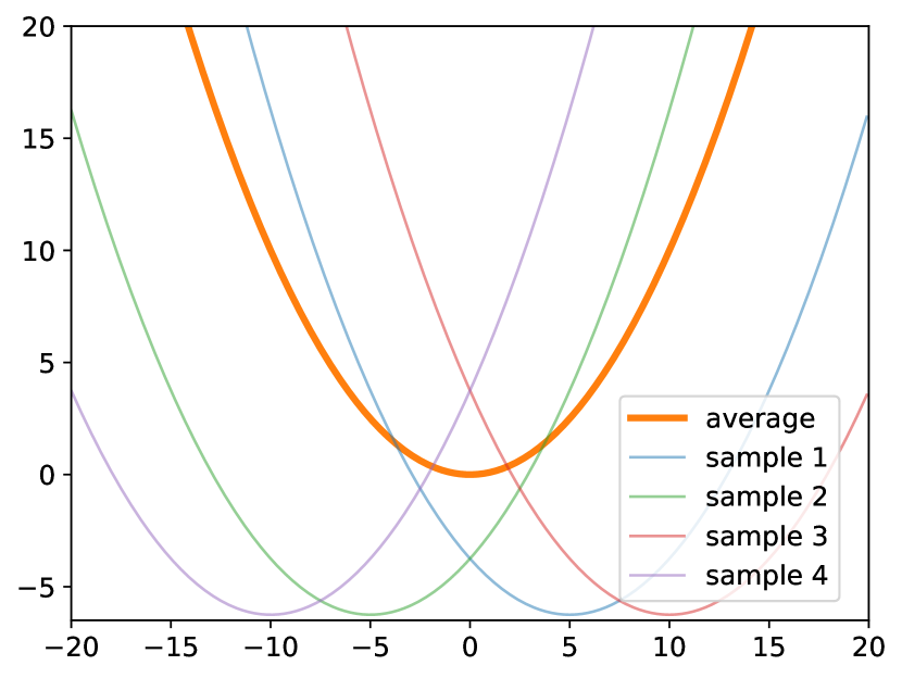
Figure C.1: An illustration of minima with low gradient variance (left) and high gradient variance (right)

The figures depict loss functions with identical average empirical loss, yet the one-sample losses are more tightly grouped in the left figure, and dispersed in the right figure. Figure C.1 illustrates that the loss function with lower gradient variance exhibits a lower sensitivity with respect to the specific sample used for evaluation. Therefore, the minima characterized by lower gradient variance may exhibit consistency in their performance when evaluated on unseen validation samples, which guarantees good generalization performance.

Lemma C.6 proves that there exists an implicit regularization effect on the variance of the one-sample gradient in SGD to improve generalization performance. It is noteworthy that as the total batch size $B$ approaches the total training sample size $N$, the regularization term diminishes rapidly, as the ratio $\frac{N-B}{N-1}$ approaches $0$ asymptotically.

Proof of Lemma C.6.

We recall the true loss function approximation of single worker SGD proposed by Smith et al. (2021):

$${\bm{L}}_{\mathbf{w}}^{\text{SGD}}=\ {\bm{L}}_{\mathbf{w}}^{\mu}\ +\frac{\eta}{4}\cdot\|\nabla{\bm{L}}_{\mathbf{w}}^{\mu}\|_{2}^{2}\ +\eta\cdot\underbrace{\frac{1}{mB^{2}}\sum_{i=0}^{m-1}\|\sum_{j=iB+1}^{iB+B}\nabla{\bm{L}}_{\mathbf{w}}^{j}-{\bm{L}}^{\mu}_{\mathbf{w}}\|_{2}^{2}}_{\text{variance of mini-batch gradients}}.$$ (C.11)

Denote $V_{j}=\nabla{\bm{L}}_{\mathbf{w}}^{j}-\nabla{\bm{L}}_{\mathbf{w}}^{\mu}$. The total variance of the mini-batch gradient in Eq. C.11 can be written as follows:

$$\frac{1}{mB^{2}}\sum_{i=0}^{m-1}\|\sum_{j=iB+1}^{iB+B}V_{j}\|_{2}^{2} =\frac{1}{mB^{2}}\sum_{i=0}^{m-1}\sum_{j_{1}=iB+1}^{iB+B}\sum_{j_{1}=iB+1}^{iB+B}V_{j_{1}}^{\top}V_{j_{2}}$$

$$=\frac{1}{mB^{2}}\sum_{i=0}^{m-1}\sum_{j_{1}=iB+1}^{iB+B}(V_{j_{1}}^{\top}V_{j_{1}}+\sum_{\begin{subarray}{c}j_{2}=iB+1\\ j_{2}\neq j_{1}\end{subarray}}^{iB+B}V_{j_{1}}^{\top}V_{j_{2}}).$$

The first part of the equation can be trivially written as $\frac{1}{mB^{2}}\sum_{i=0}^{m-1}\sum_{j_{1}=iB+1}^{iB+B}V_{j_{1}}^{\top}V_{j_{1}}=\frac{1}{NB}\sum_{j_{1}=1}^{N}V_{j_{1}}^{\top}V_{j_{1}}$. To tackle the remaining tricky part, we start by showing that

$$\frac{1}{mB^{2}}\sum_{i=0}^{m-1}\sum_{j_{1}=iB+1}^{iB+B}\sum_{\begin{subarray}{c}j_{2}=iB+1\\ j_{2}\neq j_{1}\end{subarray}}^{iB+B}V_{j_{1}}^{\top}V_{j_{2}} =\frac{1}{B^{2}}\sum_{j_{1}=1}^{B}\sum_{\begin{subarray}{c}j_{2}=1\\ j_{2}\neq j_{1}\end{subarray}}^{B}(\frac{1}{m}\sum_{i=0}^{m-1}V_{iB+j_{1}}^{\top}V_{iB+j_{2}}).$$ (C.12)

We then approximate $\frac{1}{m}\sum_{i=0}^{m-1}V_{iB+j_{1}}^{\top}V_{iB+j_{2}}$ using its expectation:

$$\frac{1}{m}\sum_{i=0}^{m-1}V_{iB+j_{1}}^{\top}V_{iB+j_{2}}=\mathbb{E}_{i}[V_{iB+j_{1}}^{\top}V_{iB+j_{2}}]+\underbrace{\left(\frac{1}{m}\sum_{i=0}^{m-1}V_{iB+j_{1}}^{\top}V_{iB+j_{2}}-\mathbb{E}_{i}[V_{iB+j_{1}}^{\top}V_{iB+j_{2}}]\right)}_{\text{bias estimator}},$$

where $\mathbb{E}_{i}$ eliminates the randomness of the sample $z_{i}$.

According to the Chebyshev’s inequality (Chebyshev, 1874; Marshall & Olkin, 1960), with a probability greater than $1-\frac{\sigma^{2}}{(m-1)\eta^{2}}=1-\frac{B\sigma^{2}}{(N-B)\eta^{2}}$, it holds that,

$$\frac{1}{m}\sum_{i=0}^{m-1}V_{iB+j_{1}}^{\top}V_{iB+j_{2}}=\mathbb{E}_{i}[V_{iB+j_{1}}^{\top}V_{iB+j_{2}}]+\mathcal{O}(\eta),$$

where $\sigma^{2}$ is the variance of random variables $V_{iB+j_{1}}^{\top}V_{iB+j_{2}}\ (i=1,\dots,m-1)$.

Substituting the sample mean approximation into Eq. C.12, we have that, with a probability greater than $1-\frac{B\sigma^{2}}{(N-B)\eta^{2}}$,

$$\frac{1}{mB^{2}}\sum_{i=0}^{m-1}\sum_{j_{1}=iB+1}^{iB+B}\sum_{\begin{subarray}{c}j_{2}=iB+1\\ j_{2}\neq j_{1}\end{subarray}}^{iB+B}V_{j_{1}}^{\top}V_{j_{2}} =\frac{B(B-1)}{B^{2}}\left(\mathbb{E}_{i}[V_{iB+j_{1}}^{\top}V_{iB+j_{2}}(1-\delta_{j_{1},j_{2}})]+\mathcal{O}{(\eta)}\right)$$

$$=\frac{B(B-1)}{B^{2}}\left(\frac{1}{N(N-1)}\sum_{i_{1}=0}^{N}\sum_{\begin{subarray}{c}i_{2}=0\\ i_{1}\neq i_{2}\end{subarray}}^{N}V_{i_{1}}^{\top}V_{i_{2}}+\mathcal{O}{(\eta)}\right),$$ (C.13)

where $\delta_{j_{1},j_{2}}$ denotes the Kronecker delta function. The derivation of the second equality is reminiscent of Subsection C.4, with a sight change of the indices.

Due to the fact that

$$\frac{1}{N(N-1)}\sum_{i_{1}=0}^{N}\sum_{i_{2}=0}^{N}V_{i_{1}}^{\top}V_{i_{2}} =\frac{1}{N-1}\|\frac{1}{N}\sum_{i_{1}=1}^{N}\nabla{\bm{L}}_{\mathbf{w}}^{i_{1}}-\nabla{\bm{L}}_{\mathbf{w}}^{\mu}\|_{2}^{2}$$

$$=\frac{1}{N-1}\|\nabla{\bm{L}}_{\mathbf{w}}^{\mu}-\nabla{\bm{L}}_{\mathbf{w}}^{\mu}\|_{2}^{2}$$

$$=0,$$

with a probability greater than $1-\frac{B\sigma^{2}}{(N-B)\eta^{2}}$, the total variance of mini-batch gradient in Eq. C.11 reads,

$$\frac{1}{mB^{2}}\sum_{i=0}^{m-1}\|\sum_{j=iB+1}^{iB+B}V_{j}\|_{2}^{2} =\frac{1}{NB}\sum_{j_{1}=1}^{N}V_{j_{1}}^{\top}V_{j_{1}}-\frac{(B-1)}{NB(N-1)}\left(\sum_{i_{1}=0}^{N}V_{i_{1}}^{\top}V_{i_{1}}\right)+\mathcal{O}{(\eta)}$$

$$=\frac{N-B}{(N-1)B}\cdot\underbrace{\frac{1}{N}\sum_{j=1}^{N}\|\nabla{\bm{L}}_{\mathbf{w}}^{j}-\nabla{\bm{L}}^{\mu}_{\mathbf{w}}\|_{2}^{2}}_{\text{variance of one-sample gradients}}+\mathcal{O}{(\eta)}.$$

According to Proposition C.4, the above results also applies for distributed centralized SGD with equivalently large batch size $B$. The proof is now complete.

∎

Theorem 3 is then established based on Lemma C.6.

Proof of Theorem 3.

According to Theorem 1, the gradient of D-SGD can be written as

$$\mathbb{E}_{\mu}[\nabla{\bm{L}}_{\mathbf{w}}^{\textnormal{D-SGD}}]=\mathbb{E}_{\epsilon\sim\mathcal{N}(0,\bm{\Xi}{\scriptstyle(t)})}[\nabla{\bm{L}}_{\mathbf{w}+\epsilon}]+\mathcal{R},$$ (C.14)

where the higher-order residual terms are absorbed in $\mathcal{R}$ for simplicity.

The mini-batch form of Eq. C.14 is

$$\hat{\nabla{\bm{L}}_{\mathbf{w}}^{\mu}}=\mathbb{E}_{\epsilon\sim\mathcal{N}(0,\bm{\Xi}{\scriptstyle(t)})}[\nabla{\bm{L}}_{\mathbf{w}+\epsilon}^{\mu}]+\mathcal{R}^{\mu}.$$

One can also derive the corresponding gradient evaluated on the $j$-th sample as

$$\hat{\nabla{\bm{L}}_{\mathbf{w}}^{j}}=\mathbb{E}_{\epsilon\sim\mathcal{N}(0,\bm{\Xi}{\scriptstyle(t)})}[\nabla{\bm{L}}_{\mathbf{w}+\epsilon}^{j}]+\mathcal{R}^{j}.$$

Replacing the original loss, the mini-batch gradient $\nabla{\bm{L}}_{\mathbf{w}}^{\mu}$ and the $j$-th sample gradient $\nabla{\bm{L}}_{\mathbf{w}}^{j}$ in Eq. C.10 with $\mathbb{E}_{\epsilon\sim\mathcal{N}(0,\bm{\Xi}{\scriptstyle(t)})}[{\bm{L}}_{\mathbf{w}+\epsilon}^{\mu}]$, $\hat{\nabla{\bm{L}}_{\mathbf{w}}^{\mu}}$ and $\hat{\nabla{\bm{L}}_{\mathbf{w}}^{j}}$, respectively, we obtain,

$${\bm{L}}_{\mathbf{w}}^{\text{D-SGD}}= \mathbb{E}_{\epsilon\sim\mathcal{N}(0,\bm{\Xi}{\scriptstyle(t)})}[{\bm{L}}_{\mathbf{w}+\epsilon}^{\mu}]+\frac{\eta}{4}\|\mathbb{E}_{\epsilon\sim\mathcal{N}(0,\bm{\Xi}{\scriptstyle(t)})}[\nabla{\bm{L}}_{\mathbf{w}+\epsilon}^{\mu}]+\nabla\mathcal{R}^{\mu}\|_{2}^{2}+\mathcal{R}^{\mu}$$

$$+\frac{\eta}{B}\cdot\frac{N-B}{(N-1)}\cdot\frac{1}{N}\sum_{j=1}^{N}\|\mathbb{E}_{\epsilon\sim\mathcal{N}(0,\bm{\Xi}{\scriptstyle(t)})}[\nabla{\bm{L}}_{\mathbf{w}+\epsilon}^{j}]-\mathbb{E}_{\epsilon\sim\mathcal{N}(0,\bm{\Xi}{\scriptstyle(t)})}[\nabla{\bm{L}}_{\mathbf{w}+\epsilon}^{\mu}]+\mathcal{R}^{j}-\mathcal{R}^{\mu}\|_{2}^{2}+\mathcal{O}{(\eta^{2})}$$

$$= {\bm{L}}_{\mathbf{w}}^{\mu}+\operatorname{Tr}({\bm{H}}^{\mu}_{\mathbf{w}}\bm{\Xi}{\scriptstyle(t)})+\frac{\eta}{4}\|\nabla{\bm{L}}_{\mathbf{w}}^{\mu}\|_{2}^{2}+\frac{\eta}{4}\operatorname{Tr}({({\bm{H}}^{\mu}_{\mathbf{w}})}^{2}\bm{\Xi}{\scriptstyle(t)})$$

$$+\frac{\eta}{B}\cdot\frac{N-B}{(N-1)}\cdot\frac{1}{N}\sum_{j=1}^{N}\left[\|\nabla{\bm{L}}_{\mathbf{w}}^{j}-\nabla{\bm{L}}_{\mathbf{w}}^{\mu}\|_{2}^{2}+\operatorname{Tr}({({\bm{H}}_{\mathbf{w}}^{j}-{\bm{H}}_{\mathbf{w}}^{\mu})}^{2}\bm{\Xi}{\scriptstyle(t)})\right]+\mathcal{R}^{A}+\mathcal{O}{(\eta^{2})},$$

with a probability greater than $1-\mathcal{O}(\frac{B}{(N-B)\eta^{2}})$, where $\mathcal{R}^{A}$ absorb all higher-order residuals. The second equality is due to first-order Taylor expansions.

The proof is now complete.

∎

References

- Andriushchenko & Flammarion (2022) Andriushchenko, M. and Flammarion, N. Towards understanding sharpness-aware minimization. In Proceedings of the 39th International Conference on Machine Learning, volume 162, pp. 639–668. PMLR, 2022.
- Andriushchenko et al. (2023) Andriushchenko, M., Bahri, D., Mobahi, H., and Flammarion, N. Sharpness-aware minimization leads to low-rank features. arXiv preprint arXiv:2305.16292, 2023.
- Assran et al. (2019) Assran, M., Loizou, N., Ballas, N., and Rabbat, M. Stochastic gradient push for distributed deep learning. In International Conference on Machine Learning, 2019.
- Bahri et al. (2022) Bahri, D., Mobahi, H., and Tay, Y. Sharpness-aware minimization improves language model generalization. In Proceedings of the 60th Annual Meeting of the Association for Computational Linguistics (Volume 1: Long Papers), pp. 7360–7371. Association for Computational Linguistics, 2022.
- Bassily et al. (2020) Bassily, R., Feldman, V., Guzmán, C., and Talwar, K. Stability of stochastic gradient descent on nonsmooth convex losses. In Advances in Neural Information Processing Systems, 2020.
- Beltrán et al. (2022) Beltrán, E. T. M., Pérez, M. Q., Sánchez, P. M. S., Bernal, S. L., Bovet, G., Pérez, M. G., Pérez, G. M., and Celdrán, A. H. Decentralized federated learning: Fundamentals, state-of-the-art, frameworks, trends, and challenges. arXiv preprint arXiv:2211.08413, 2022.
- Bisla et al. (2022) Bisla, D., Wang, J., and Choromanska, A. Low-pass filtering SGD for recovering flat optima in the deep learning optimization landscape. In International Conference on Artificial Intelligence and Statistics, pp. 8299–8339. PMLR, 2022.
- Bornstein et al. (2023) Bornstein, M., Rabbani, T., Wang, E. Z., Bedi, A., and Huang, F. SWIFT: Rapid decentralized federated learning via wait-free model communication. In The Eleventh International Conference on Learning Representations, 2023.
- Borzunov et al. (2022) Borzunov, A., Baranchuk, D., Dettmers, T., Ryabinin, M., Belkada, Y., Chumachenko, A., Samygin, P., and Raffel, C. Petals: Collaborative inference and fine-tuning of large models. arXiv preprint arXiv:2209.01188, 2022.
- Bottou et al. (2018) Bottou, L., Curtis, F. E., and Nocedal, J. Optimization methods for large-scale machine learning. Siam Review, 60(2):223–311, 2018.
- Boyd et al. (2004) Boyd, S., Boyd, S. P., and Vandenberghe, L. Convex optimization. Cambridge university press, 2004.
- Cao et al. (2023) Cao, Y., Rizk, E., Vlaski, S., and Sayed, A. H. Decentralized adversarial training over graphs. arXiv preprint arXiv:2303.13326, 2023.
- Cauchy et al. (1847) Cauchy, A. et al. Méthode générale pour la résolution des systemes d’équations simultanées. Comp. Rend. Sci. Paris, 25(1847):536–538, 1847.
- Chaudhari et al. (2019) Chaudhari, P., Choromanska, A., Soatto, S., LeCun, Y., Baldassi, C., Borgs, C., Chayes, J., Sagun, L., and Zecchina, R. Entropy-SGD: Biasing gradient descent into wide valleys. Journal of Statistical Mechanics: Theory and Experiment, 2019(12):124018, 2019.
- Chebyshev (1874) Chebyshev, P. L. Sur les valeurs limites des intégrales. Imprimerie de Gauthier-Villars Paris, 1874.
- Chen & Huo (2016) Chen, K. and Huo, Q. Scalable training of deep learning machines by incremental block training with intra-block parallel optimization and blockwise model-update filtering. In 2016 IEEE International Conference on Acoustics, Speech and Signal Processing (ICASSP), pp. 5880–5884. IEEE Press, 2016.
- Chen et al. (2022) Chen, X., Hsieh, C.-J., and Gong, B. When vision transformers outperform resnets without pre-training or strong data augmentations. In International Conference on Learning Representations, 2022.
- Chor et al. (2023) Chor, R., Sefidgaran, M., and Zaidi, A. More communication does not result in smaller generalization error in federated learning. arXiv preprint arXiv:2304.12216, 2023.
- Davis (1962) Davis, C. The norm of the schur product operation. Numerische Mathematik, 4:343–344, 1962.
- De Bruijn (1981) De Bruijn, N. G. Asymptotic methods in analysis, volume 4. Courier Corporation, 1981.
- Dean et al. (2012) Dean, J., Corrado, G., Monga, R., Chen, K., Devin, M., Mao, M., Ranzato, M., Senior, A., Tucker, P., Yang, K., et al. Large scale distributed deep networks. Advances in neural information processing systems, 2012.
- Deng et al. (2023) Deng, X., Sun, T., Li, S., and Li, D. Stability-based generalization analysis of the asynchronous decentralized sgd. In Proceedings of the AAAI Conference on Artificial Intelligence, 2023.
- Dosovitskiy et al. (2021) Dosovitskiy, A., Beyer, L., Kolesnikov, A., Weissenborn, D., Zhai, X., Unterthiner, T., Dehghani, M., Minderer, M., Heigold, G., Gelly, S., Uszkoreit, J., and Houlsby, N. An image is worth 16x16 words: Transformers for image recognition at scale. In International Conference on Learning Representations, 2021.
- Du et al. (2022) Du, J., Yan, H., Feng, J., Zhou, J. T., Zhen, L., Goh, R. S. M., and Tan, V. Efficient sharpness-aware minimization for improved training of neural networks. In International Conference on Learning Representations, 2022.
- Erdélyi (1956) Erdélyi, A. Asymptotic expansions. Number 3. Courier Corporation, 1956.
- Farhadkhani et al. (2023) Farhadkhani, S., Guerraoui, R., Gupta, N., Hoang, L. N., Pinot, R., and Stephan, J. Robust collaborative learning with linear gradient overhead. In International Conference on Machine Learning, 2023.
- Foret et al. (2021) Foret, P., Kleiner, A., Mobahi, H., and Neyshabur, B. Sharpness-aware minimization for efficiently improving generalization. In International Conference on Learning Representations, 2021.
- Geiping et al. (2020) Geiping, J., Bauermeister, H., Dröge, H., and Moeller, M. Inverting gradients - how easy is it to break privacy in federated learning? In Advances in Neural Information Processing Systems, 2020.
- Goyal et al. (2017) Goyal, P., Dollár, P., Girshick, R., Noordhuis, P., Wesolowski, L., Kyrola, A., Tulloch, A., Jia, Y., and He, K. Accurate, large minibatch sgd: Training imagenet in 1 hour. arXiv preprint arXiv:1706.02677, 2017.
- Gu et al. (2023) Gu, X., Lyu, K., Huang, L., and Arora, S. Why (and when) does local SGD generalize better than SGD? In International Conference on Learning Representations, 2023.
- Gurbuzbalaban et al. (2022) Gurbuzbalaban, M., Hu, Y., Simsekli, U., Yuan, K., and Zhu, L. Heavy-tail phenomenon in decentralized sgd. arXiv preprint arXiv:2205.06689, 2022.
- He et al. (2019) He, F., Liu, T., and Tao, D. Control batch size and learning rate to generalize well: Theoretical and empirical evidence. In Advances in Neural Information Processing Systems, pp. 1143–1152, 2019.
- He et al. (2016a) He, K., Zhang, X., Ren, S., and Sun, J. Deep residual learning for image recognition. In Proceedings of the IEEE conference on computer vision and pattern recognition, 2016a.
- He et al. (2016b) He, K., Zhang, X., Ren, S., and Sun, J. Identity mappings in deep residual networks. In European conference on computer vision. Springer, 2016b.
- Hochreiter & Schmidhuber (1997) Hochreiter, S. and Schmidhuber, J. Flat minima. Neural computation, 9(1):1–42, 1997.
- Hoffer et al. (2017) Hoffer, E., Hubara, I., and Soudry, D. Train longer, generalize better: closing the generalization gap in large batch training of neural networks. Advances in neural information processing systems, 2017.
- Huang et al. (2017) Huang, G., Liu, Z., van der Maaten, L., and Weinberger, K. Q. Densely connected convolutional networks. In Proceedings of the IEEE Conference on Computer Vision and Pattern Recognition (CVPR), July 2017.
- Ibayashi & Imaizumi (2021) Ibayashi, H. and Imaizumi, M. Exponential escape efficiency of sgd from sharp minima in non-stationary regime. arXiv preprint arXiv:2111.04004, 2021.
- Ioffe & Szegedy (2015) Ioffe, S. and Szegedy, C. Batch normalization: Accelerating deep network training by reducing internal covariate shift. In International conference on machine learning, 2015.
- Izmailov et al. (2018) Izmailov, P., Podoprikhin, D., Garipov, T., Vetrov, D., and Wilson, A. G. Averaging weights leads to wider optima and better generalization. arXiv preprint arXiv:1803.05407, 2018.
- Jiang et al. (2020) Jiang, Y., Neyshabur*, B., Mobahi, H., Krishnan, D., and Bengio, S. Fantastic generalization measures and where to find them. In International Conference on Learning Representations, 2020.
- Keskar et al. (2017) Keskar, N. S., Mudigere, D., Nocedal, J., Smelyanskiy, M., and Tang, P. T. P. On large-batch training for deep learning: Generalization gap and sharp minima. In International Conference on Learning Representations. PMLR, 2017.
- Kim et al. (2023) Kim, H., Park, J., Choi, Y., and Lee, J. Stability analysis of sharpness-aware minimization. arXiv preprint arXiv:2301.06308, 2023.
- Kim et al. (2022) Kim, M., Li, D., Hu, S. X., and Hospedales, T. Fisher SAM: Information geometry and sharpness aware minimisation. In Proceedings of the 39th International Conference on Machine Learning, volume 162 of Proceedings of Machine Learning Research, pp. 11148–11161. PMLR, 2022.
- Koloskova et al. (2020) Koloskova, A., Loizou, N., Boreiri, S., Jaggi, M., and Stich, S. A unified theory of decentralized SGD with changing topology and local updates. In International Conference on Machine Learning, 2020.
- Kong et al. (2021) Kong, L., Lin, T., Koloskova, A., Jaggi, M., and Stich, S. Consensus control for decentralized deep learning. In International Conference on Machine Learning. PMLR, 2021.
- Krizhevsky et al. (2009) Krizhevsky, A., Hinton, G., et al. Learning multiple layers of features from tiny images (tech. rep.). University of Toronto, 2009.
- Krizhevsky et al. (2017) Krizhevsky, A., Sutskever, I., and Hinton, G. E. Imagenet classification with deep convolutional neural networks. Communications of the ACM, 60(6):84–90, 2017.
- Kwon et al. (2021) Kwon, J., Kim, J., Park, H., and Choi, I. K. Asam: Adaptive sharpness-aware minimization for scale-invariant learning of deep neural networks. In International Conference on Machine Learning, pp. 5905–5914. PMLR, 2021.
- Le & Yang (2015) Le, Y. and Yang, X. Tiny imagenet visual recognition challenge. CS 231N, 2015.
- Le Bars et al. (2023) Le Bars, B., Bellet, A., Tommasi, M., Lavoie, E., and Kermarrec, A.-M. Refined convergence and topology learning for decentralized sgd with heterogeneous data. In Proceedings of The 26th International Conference on Artificial Intelligence and Statistics, volume 206, pp. 1672–1702. PMLR, 25–27 Apr 2023.
- Li et al. (2018) Li, H., Xu, Z., Taylor, G., Studer, C., and Goldstein, T. Visualizing the loss landscape of neural nets. Advances in neural information processing systems, 2018.
- Li et al. (2014) Li, M., Andersen, D. G., Smola, A. J., and Yu, K. Communication efficient distributed machine learning with the parameter server. Advances in Neural Information Processing Systems, 2014.
- Li et al. (2022) Li, S., Zhou, T., Tian, X., and Tao, D. Learning to collaborate in decentralized learning of personalized models. In Proceedings of the IEEE/CVF Conference on Computer Vision and Pattern Recognition, pp. 9766–9775, 2022.
- Li et al. (2021) Li, Z., Malladi, S., and Arora, S. On the validity of modeling sgd with stochastic differential equations (sdes). Advances in Neural Information Processing Systems, 2021.
- Lian et al. (2017) Lian, X., Zhang, C., Zhang, H., Hsieh, C.-J., Zhang, W., and Liu, J. Can decentralized algorithms outperform centralized algorithms? a case study for decentralized parallel stochastic gradient descent. In Advances in Neural Information Processing Systems, 2017.
- Lian et al. (2018) Lian, X., Zhang, W., Zhang, C., and Liu, J. Asynchronous decentralized parallel stochastic gradient descent. In International Conference on Machine Learning, 2018.
- Liu et al. (2021) Liu, K., Ziyin, L., and Ueda, M. Noise and fluctuation of finite learning rate stochastic gradient descent. In International Conference on Machine Learning. PMLR, 2021.
- Liu et al. (2022a) Liu, Y., Mai, S., Chen, X., Hsieh, C.-J., and You, Y. Towards efficient and scalable sharpness-aware minimization. In Proceedings of the IEEE/CVF Conference on Computer Vision and Pattern Recognition, pp. 12360–12370, 2022a.
- Liu et al. (2022b) Liu, Y., Mai, S., Cheng, M., Chen, X., Hsieh, C.-J., and You, Y. Random sharpness-aware minimization. In Oh, A. H., Agarwal, A., Belgrave, D., and Cho, K. (eds.), Advances in Neural Information Processing Systems, 2022b.
- Liu et al. (2022c) Liu, Z., Kangqiao, L., Takashi, M., and Masahito, U. Strength of minibatch noise in SGD. In International Conference on Learning Representations, 2022c.
- Lopes & Sayed (2008) Lopes, C. G. and Sayed, A. H. Diffusion least-mean squares over adaptive networks: Formulation and performance analysis. IEEE Transactions on Signal Processing, 2008.
- Lu et al. (2011) Lu, J., Tang, C. Y., Regier, P. R., and Bow, T. D. Gossip algorithms for convex consensus optimization over networks. IEEE Transactions on Automatic Control, 2011.
- Lu & Wu (2020) Lu, S. and Wu, C. W. Decentralized stochastic non-convex optimization over weakly connected time-varying digraphs. In ICASSP 2020-2020 IEEE International Conference on Acoustics, Speech and Signal Processing (ICASSP), 2020.
- Lu & Sa (2023) Lu, Y. and Sa, C. D. Decentralized learning: Theoretical optimality and practical improvements. Journal of Machine Learning Research, 24(93):1–62, 2023.
- Ma et al. (2022) Ma, C., Kunin, D., Wu, L., and Ying, L. Beyond the quadratic approximation: The multiscale structure of neural network loss landscapes. Journal of Machine Learning, 1(3):247–267, 2022.
- MacKay (1992) MacKay, D. J. A practical bayesian framework for backpropagation networks. Neural computation, 4(3):448–472, 1992.
- Marshall & Olkin (1960) Marshall, A. W. and Olkin, I. Multivariate chebyshev inequalities. The Annals of Mathematical Statistics, pp. 1001–1014, 1960.
- Marshall et al. (1979) Marshall, A. W., Olkin, I., and Arnold, B. C. Inequalities: theory of majorization and its applications. Springer, 1979.
- McMahan et al. (2017) McMahan, B., Moore, E., Ramage, D., Hampson, S., and Arcas, B. A. y. Communication-Efficient Learning of Deep Networks from Decentralized Data. In Proceedings of the 20th International Conference on Artificial Intelligence and Statistics, volume 54, pp. 1273–1282. PMLR, 2017.
- Merikoski (1984) Merikoski, J. K. On the trace and the sum of elements of a matrix. Linear algebra and its applications, 60:177–185, 1984.
- Mi et al. (2022) Mi, P., Shen, L., Ren, T., Zhou, Y., Sun, X., Ji, R., and Tao, D. Make sharpness-aware minimization stronger: A sparsified perturbation approach. In Oh, A. H., Agarwal, A., Belgrave, D., and Cho, K. (eds.), Advances in Neural Information Processing Systems, 2022.
- Mueller & Hein (2022) Mueller, M. and Hein, M. Perturbing batchnorm and only batchnorm benefits sharpness-aware minimization. In Has it Trained Yet? NeurIPS 2022 Workshop, 2022.
- Möllenhoff & Khan (2023) Möllenhoff, T. and Khan, M. E. SAM as an optimal relaxation of bayes. In The Eleventh International Conference on Learning Representations, 2023.
- Nadiradze et al. (2021) Nadiradze, G., Sabour, A., Davies, P., Li, S., and Alistarh, D. Asynchronous decentralized sgd with quantized and local updates. Advances in Neural Information Processing Systems, 2021.
- Narayanan et al. (2021) Narayanan, D., Shoeybi, M., Casper, J., LeGresley, P., Patwary, M., Korthikanti, V., Vainbrand, D., Kashinkunti, P., Bernauer, J., Catanzaro, B., et al. Efficient large-scale language model training on gpu clusters using megatron-lm. In Proceedings of the International Conference for High Performance Computing, Networking, Storage and Analysis, pp. 1–15, 2021.
- Nedic (2020) Nedic, A. Distributed gradient methods for convex machine learning problems in networks: Distributed optimization. IEEE Signal Processing Magazine, 2020.
- Nedić & Olshevsky (2014) Nedić, A. and Olshevsky, A. Distributed optimization over time-varying directed graphs. IEEE Transactions on Automatic Control, 60(3):601–615, 2014.
- Nedic & Ozdaglar (2009) Nedic, A. and Ozdaglar, A. Distributed subgradient methods for multi-agent optimization. IEEE Transactions on Automatic Control, 54(1):48–61, 2009.
- Neyshabur et al. (2017) Neyshabur, B., Bhojanapalli, S., Mcallester, D., and Srebro, N. Exploring generalization in deep learning. In Advances in Neural Information Processing Systems, 2017.
- Paszke et al. (2019) Paszke, A., Gross, S., Massa, F., Lerer, A., Bradbury, J., Chanan, G., Killeen, T., Lin, Z., Gimelshein, N., Antiga, L., et al. Pytorch: An imperative style, high-performance deep learning library. Advances in neural information processing systems, 2019.
- Reddi et al. (2021) Reddi, S. J., Charles, Z., Zaheer, M., Garrett, Z., Rush, K., Konečný, J., Kumar, S., and McMahan, H. B. Adaptive federated optimization. In International Conference on Learning Representations, 2021.
- Rissanen (1983) Rissanen, J. A universal prior for integers and estimation by minimum description length. The Annals of statistics, 11(2):416–431, 1983.
- Robbins (1951) Robbins, H. E. A stochastic approximation method. Annals of Mathematical Statistics, 22:400–407, 1951.
- Rockafellar & Wets (2009) Rockafellar, R. T. and Wets, R. J.-B. Variational analysis, volume 317. Springer Science & Business Media, 2009.
- Rudin et al. (1976) Rudin, W. et al. Principles of mathematical analysis. McGraw-hill New York, 1976.
- Seneta (2006) Seneta, E. Non-negative matrices and Markov chains. Springer Science & Business Media, 2006.
- Shallue et al. (2019) Shallue, C. J., Lee, J., Antognini, J., Sohl-Dickstein, J., Frostig, R., and Dahl, G. E. Measuring the effects of data parallelism on neural network training. Journal of Machine Learning Research, 20(112):1–49, 2019.
- Shamir & Srebro (2014) Shamir, O. and Srebro, N. Distributed stochastic optimization and learning. In 2014 52nd Annual Allerton Conference on Communication, Control, and Computing (Allerton), 2014.
- Shen et al. (2023) Shen, L., Sun, Y., Yu, Z., Ding, L., Tian, X., and Tao, D. On efficient training of large-scale deep learning models: A literature review. arXiv preprint arXiv:2304.03589, 2023.
- Shi et al. (2015) Shi, W., Ling, Q., Wu, G., and Yin, W. Extra: An exact first-order algorithm for decentralized consensus optimization. SIAM Journal on Optimization, 2015.
- Shi et al. (2023a) Shi, Y., Liu, Y., Sun, Y., Lin, Z., Shen, L., Wang, X., and Tao, D. Towards more suitable personalization in federated learning via decentralized partial model training. arXiv preprint arXiv:2305.15157, 2023a.
- Shi et al. (2023b) Shi, Y., Shen, L., Wei, K., Sun, Y., Yuan, B., Wang, X., and Tao, D. Improving the model consistency of decentralized federated learning. In Proceedings of the 40th International Conference on Machine Learning, pp. 31269–31291. PMLR, 2023b.
- Smith (2017) Smith, L. N. Cyclical learning rates for training neural networks. In 2017 IEEE winter conference on applications of computer vision (WACV), pp. 464–472. IEEE, 2017.
- Smith et al. (2020) Smith, S., Elsen, E., and De, S. On the generalization benefit of noise in stochastic gradient descent. In International Conference on Machine Learning. PMLR, 2020.
- Smith et al. (2021) Smith, S. L., Dherin, B., Barrett, D., and De, S. On the origin of implicit regularization in stochastic gradient descent. In International Conference on Learning Representations, 2021.
- Song et al. (2022) Song, Z., Li, W., Jin, K., Shi, L., Yan, M., Yin, W., and Yuan, K. Communication-efficient topologies for decentralized learning with $o(1)$ consensus rate. In Oh, A. H., Agarwal, A., Belgrave, D., and Cho, K. (eds.), Advances in Neural Information Processing Systems, 2022.
- Sun et al. (2021) Sun, T., Li, D., and Wang, B. Stability and generalization of decentralized stochastic gradient descent. In Proceedings of the AAAI Conference on Artificial Intelligence, volume 35, pp. 9756–9764, 2021.
- Taheri et al. (2020) Taheri, H., Mokhtari, A., Hassani, H., and Pedarsani, R. Quantized decentralized stochastic learning over directed graphs. In International Conference on Machine Learning. PMLR, 2020.
- Tang et al. (2018) Tang, H., Lian, X., Yan, M., Zhang, C., and Liu, J. D2: Decentralized training over decentralized data. In International Conference on Machine Learning. PMLR, 2018.
- Tsitsiklis et al. (1986) Tsitsiklis, J., Bertsekas, D., and Athans, M. Distributed asynchronous deterministic and stochastic gradient optimization algorithms. IEEE transactions on automatic control, 31(9):803–812, 1986.
- Tsitsiklis (1984) Tsitsiklis, J. N. Problems in decentralized decision making and computation. Technical report, Massachusetts Inst of Tech Cambridge Lab for Information and Decision Systems, 1984.
- Ujváry et al. (2022) Ujváry, S., Telek, Z., Kerekes, A., Mészáros, A., and Huszár, F. Rethinking sharpness-aware minimization as variational inference. In OPT 2022: Optimization for Machine Learning (NeurIPS 2022 Workshop), 2022.
- Vershynin (2018) Vershynin, R. High-dimensional probability: An introduction with applications in data science, volume 47. Cambridge university press, 2018.
- Vogels et al. (2021) Vogels, T., He, L., Koloskova, A., Karimireddy, S. P., Lin, T., Stich, S. U., and Jaggi, M. Relaysum for decentralized deep learning on heterogeneous data. Advances in Neural Information Processing Systems, 34:28004–28015, 2021.
- Von Neumann (1937) Von Neumann, J. Some matrix-inequalities and metrization of matric space. 1937.
- Wang et al. (2020) Wang, J., Liu, Q., Liang, H., Joshi, G., and Poor, H. V. Tackling the objective inconsistency problem in heterogeneous federated optimization. Advances in neural information processing systems, 33:7611–7623, 2020.
- Wang et al. (2022) Wang, J., Das, R., Joshi, G., Kale, S., Xu, Z., and Zhang, T. On the unreasonable effectiveness of federated averaging with heterogeneous data. arXiv preprint arXiv:2206.04723, 2022.
- Wang et al. (2023) Wang, Z., Lee, J., and Lei, Q. Reconstructing training data from model gradient, provably. In International Conference on Artificial Intelligence and Statistics, pp. 6595–6612. PMLR, 2023.
- Warnat-Herresthal et al. (2021) Warnat-Herresthal, S., Schultze, H., Shastry, K. L., Manamohan, S., Mukherjee, S., Garg, V., Sarveswara, R., Händler, K., Pickkers, P., Aziz, N. A., et al. Swarm learning for decentralized and confidential clinical machine learning. Nature, 2021.
- Wen et al. (2023) Wen, K., Ma, T., and Li, Z. How sharpness-aware minimization minimizes sharpness? In International Conference on Learning Representations, 2023.
- Wu et al. (2020) Wu, D., Xia, S.-T., and Wang, Y. Adversarial weight perturbation helps robust generalization. Advances in Neural Information Processing Systems, 33:2958–2969, 2020.
- Wu & Su (2023) Wu, L. and Su, W. J. The implicit regularization of dynamical stability in stochastic gradient descent. In International Conference on Machine Learning. PMLR, 2023.
- Xiao & Boyd (2004) Xiao, L. and Boyd, S. Fast linear iterations for distributed averaging. Systems & Control Letters, 2004.
- Xu et al. (2021) Xu, J., Zhang, W., and Wang, F. A(dp)2sgd: Asynchronous decentralized parallel stochastic gradient descent with differential privacy. IEEE Transactions on Pattern Analysis and Machine Intelligence, 2021.
- Yang et al. (2020) Yang, Z., Gang, A., and Bajwa, W. U. Adversary-resilient distributed and decentralized statistical inference and machine learning: An overview of recent advances under the byzantine threat model. IEEE Signal Processing Magazine, 37(3):146–159, 2020.
- Yin et al. (2018) Yin, D., Pananjady, A., Lam, M., Papailiopoulos, D., Ramchandran, K., and Bartlett, P. Gradient diversity: a key ingredient for scalable distributed learning. In Proceedings of the Twenty-First International Conference on Artificial Intelligence and Statistics, volume 84, pp. 1998–2007. PMLR, 2018.
- Yin et al. (2021) Yin, H., Mallya, A., Vahdat, A., Alvarez, J. M., Kautz, J., and Molchanov, P. See through gradients: Image batch recovery via gradinversion. In Proceedings of the IEEE/CVF Conference on Computer Vision and Pattern Recognition (CVPR), 2021.
- Ying et al. (2021a) Ying, B., Yuan, K., Chen, Y., Hu, H., Pan, P., and Yin, W. Exponential graph is provably efficient for decentralized deep training. In Advances in Neural Information Processing Systems, 2021a.
- Ying et al. (2021b) Ying, B., Yuan, K., Hu, H., Chen, Y., and Yin, W. Bluefog: Make decentralized algorithms practical for optimization and deep learning. arXiv preprint arXiv:2111.04287, 2021b.
- You et al. (2017) You, Y., Gitman, I., and Ginsburg, B. Large batch training of convolutional networks. arXiv preprint arXiv:1708.03888, 2017.
- You et al. (2018) You, Y., Zhang, Z., Hsieh, C.-J., Demmel, J., and Keutzer, K. Imagenet training in minutes. In Proceedings of the 47th International Conference on Parallel Processing. Association for Computing Machinery, 2018.
- You et al. (2020) You, Y., Li, J., Reddi, S., Hseu, J., Kumar, S., Bhojanapalli, S., Song, X., Demmel, J., Keutzer, K., and Hsieh, C.-J. Large batch optimization for deep learning: Training bert in 76 minutes. In International Conference on Learning Representations, 2020.
- Yuan et al. (2022) Yuan, B., He, Y., Davis, J. Q., Zhang, T., Dao, T., Chen, B., Liang, P., Re, C., and Zhang, C. Decentralized training of foundation models in heterogeneous environments. In Oh, A. H., Agarwal, A., Belgrave, D., and Cho, K. (eds.), Advances in Neural Information Processing Systems, 2022.
- Yuan et al. (2021) Yuan, K., Chen, Y., Huang, X., Zhang, Y., Pan, P., Xu, Y., and Yin, W. Decentlam: Decentralized momentum sgd for large-batch deep training. In Proceedings of the IEEE/CVF International Conference on Computer Vision, pp. 3029–3039, 2021.
- Zellner (1988) Zellner, A. Optimal information processing and bayes’s theorem. The American Statistician, 42(4):278–280, 1988.
- Zhang et al. (2020) Zhang, W., Cui, X., Kayi, A., Liu, M., Finkler, U., Kingsbury, B., Saon, G., Mroueh, Y., Buyuktosunoglu, A., Das, P., Kung, D. S., and Picheny, M. Improving efficiency in large-scale decentralized distributed training. ICASSP 2020 - 2020 IEEE International Conference on Acoustics, Speech and Signal Processing (ICASSP), pp. 3022–3026, 2020.
- Zhang et al. (2021) Zhang, W., Liu, M., Feng, Y., Cui, X., Kingsbury, B., and Tu, Y. Loss landscape dependent self-adjusting learning rates in decentralized stochastic gradient descent. arXiv preprint arXiv:2112.01433, 2021.
- Zheng et al. (2021) Zheng, Y., Zhang, R., and Mao, Y. Regularizing neural networks via adversarial model perturbation. In Proceedings of the IEEE/CVF Conference on Computer Vision and Pattern Recognition, pp. 8156–8165, 2021.
- Zhu et al. (2019a) Zhu, L., Liu, Z., and Han, S. Deep leakage from gradients. In Advances in Neural Information Processing Systems, 2019a.
- Zhu et al. (2022) Zhu, T., He, F., Zhang, L., Niu, Z., Song, M., and Tao, D. Topology-aware generalization of decentralized sgd. In International Conference on Machine Learning. PMLR, 2022.
- Zhu et al. (2019b) Zhu, Z., Wu, J., Yu, B., Wu, L., and Ma, J. The anisotropic noise in stochastic gradient descent: Its behavior of escaping from sharp minima and regularization effects. In International Conference on Machine Learning. PMLR, 2019b.
- Zhuang et al. (2022) Zhuang, J., Gong, B., Yuan, L., Cui, Y., Adam, H., Dvornek, N. C., sekhar tatikonda, s Duncan, J., and Liu, T. Surrogate gap minimization improves sharpness-aware training. In International Conference on Learning Representations, 2022.