Degenerate flat bands in twisted bilayer graphene

Abstract.

We prove that in the chiral limit of the Bistritzer-MacDonald Hamiltonian, there exist magic angles at which the Hamiltonian exhibits flat bands of multiplicity four instead of two. We analyze the structure of the Bloch functions associated with the four bands, compute the corresponding Chern number, and show that there exist infinitely many degenerate magic angles for a generic choice of tunnelling potentials. Moreover, we demonstrate that the Hamiltonian, when subject to typical tunnelling potentials, exclusively yields flat bands of either twofold or fourfold multiplicity at each magic angle.

1. Introduction and statement of results

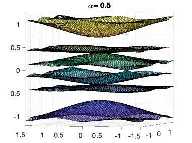
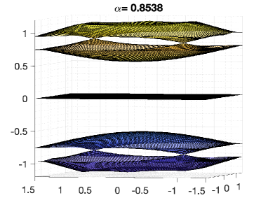
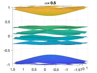
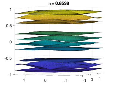
Figure 8. Bands of Hamiltonian at $\alpha=0.5$ (left) and $\alpha=0.8538$ (right) with potential $U_{2}$ (1.8). Bands of full continuum Bistritzer-MacDonald Hamiltonian with same $\alpha$ and $\beta=0.7\alpha$ with potential $U_{2}$ (1.8) and anti-chiral potential $V(z):=2\partial_{z}U_{2}(z)$.

Twisted bilayer graphene is a material consisting of two stacked graphene layers which are twisted with respect to each other by an angle $\theta.$ It has been predicted theoretically [BiMa11] that at a certain angle, the bands at zero energy become flat and strongly correlated electron effects dominate. This has then been experimentally confirmed that at this magic angle, the material exhibits phenomena such as superconductivity and a quantum Hall effect without external magnetic fields [Cao18, Ser19, Yan18]. Theoretically [TKV19] more magic angles have been expected. Perhaps contrary to common beliefs, we show that flat bands of higher multiplicity are ubiquitous in this model of bilayer graphene. Higher multiplicity bands have recently also been theoretically observed in models of twisted trilayer graphene [PT23, De23]. We verify numerically that the presence of higher degenerate (almost flat) bands close to zero energy is also valid for the full (not just chiral) model, see Figure 8.

The model we consider is based on the Bistritzer MacDonald Hamiltonian [BiMa11, CGG22, Wa^∗22] and its chiral limit of Tarnopolsky–Kruchkov–Vishwanath [TKV19]:

$$H(\alpha)=\begin{pmatrix}0&D(\alpha)^{*}\\ D(\alpha)&0\end{pmatrix}\text{ with }D(\alpha)=\begin{pmatrix}2D_{\bar{z}}&\alpha U_{+}(z)\\ \alpha U_{-}(z)&2D_{\bar{z}}\end{pmatrix}$$ (1.1)

where the parameter $\alpha$ is proportional to the inverse relative twisting angle. With $\omega=e^{2\pi i/3}$ and $\mathbf{a}={4\pi i}(a_{1}\omega+a_{2}\bar{\omega})$, $a_{j}\in\mathbb{Z}$, we assume that

$$U_{\pm}(z+\mathbf{a})=\omega^{\mp(a_{1}+a_{2})}U(z),\quad U_{\pm}(\omega z)=\omega U_{\pm}(z).$$ (1.2)

The most important case is given by

$$U_{+}(z)=U(z),\ \ \ U_{-}(z)=U(-z),\ \ \ \overline{U(\bar{z})}=U(z),$$ (1.3)

see (1.8) for concrete examples.

Floquet theory for the Hamiltonian (1.1) is based on moiré translations:

$${\mathscr{L}}_{\mathbf{a}}u:=\begin{pmatrix}\omega^{-(a_{1}+a_{2})}&0\\ 0&\omega^{a_{1}+a_{2}}\end{pmatrix}u(z+\mathbf{a}),\ \ \ \mathbf{a}={4\pi i}(a_{1}\omega+a_{2}\bar{\omega}).$$ (1.4)

The action is extended diagonally to $\mathbb{C}^{4}=\mathbb{C}^{2}\times\mathbb{C}^{2}$-valued functions and we $\mathscr{L}_{\mathbf{a}}H(\alpha)=H(\alpha)\mathscr{L}_{\mathbf{a}}$.

The Floquet spectrum is given by

$$\begin{gathered}H(\alpha)u=Eu,\ \ u\in H^{1}_{k}\ \ \ H^{s}_{k}:=L^{2}_{k}\cap H^{s}_{\rm{loc}},\\ L^{2}_{k}:=\{u=L^{2}_{\rm{loc}}(\mathbb{C};\mathbb{C}^{4}):\mathscr{L}_{\mathbf{a}}u=e^{i\langle k,\mathbf{a}\rangle}u\},\quad\langle z,w\rangle:=\operatorname{Re}(z\bar{w}).\end{gathered}$$ (1.5)

The spectrum is discrete and symmetric with respect to the origin and we index it as follows (with $\mathbb{Z}^{*}:=\mathbb{Z}\setminus\{0\}$)

$$\begin{gathered}\{E_{j}(\alpha,k)\}_{j\in\mathbb{Z}^{*}},\ \ \ E_{j}(\alpha,k)=-E_{-j}(\alpha,k),\\ 0\leq E_{1}(\alpha,k)\leq E_{2}(\alpha,k)\leq\cdots,\ \ \ E_{1}(\alpha,K)=E_{1}(\alpha,-K)=0,\end{gathered}$$ (1.6)

see [BHZ22b, §2] for more details. The points $K,-K$, $K=i$, are called the Dirac points and are typically denoted by $K$ and $K^{\prime}$ in the physics literature.

Definition (Magic angles and their multiplicities). A value of $\alpha$ in (1.1) is called magical if $H(\alpha)$ has a flat band at zero

$$E_{1}(\alpha,k)\equiv 0,\ \ k\in\mathbb{C}.$$

The set of magic $\alpha$’s is denoted by $\mathcal{A}$ or $\mathcal{A}(U)$ if we specify the dependence on the potential. The multiplicity of a magic $\alpha$ is defined as

$$m(\alpha)=m_{U}(\alpha)=\min\{j>0:\max_{k}E_{j+1}(\alpha,k)>0\}.$$ (1.7)

Magic angles are (up to physical constants) reciprocals of $\alpha\in\mathcal{A}$.

Because of the symmetry of the spectrum (1.6) simple $\alpha$’s correspond flat bands of multiplicity $2$ and double $\alpha$’s, to flat bands of multiplicity 4.

Examples of $U$’s satisfying (1.2) and (1.3) are given by

$$U_{1}(z)=\sum_{\ell=0}^{2}\omega^{\ell}e^{\frac{1}{2}({z\bar{\omega}^{\ell}-\bar{z}\omega^{\ell}})}\ \text{ and }\ U_{2}(z)=\tfrac{1}{\sqrt{2}}\Big{(}U_{1}(z)-\sum_{\ell=0}^{2}\omega^{\ell}e^{-(z\bar{\omega}^{\ell}-\bar{z}\omega^{\ell})}\Big{)}.$$ (1.8)

Numerical experiments suggest that these two potentials exhibit flat bands of different multiplicities:

$$m_{U_{j}}(\alpha)=j,\ \ \alpha\in\mathcal{A}_{U_{j}}\cap\mathbb{R},\ \ j=1,2,$$ (1.9)

see Figure 1. We show (see Theorem 2 below) that the potential $U_{1}$ (the Bistritzer–MacDonald potential) has infinitely many (complex) degenerate magic $\alpha$’s. While in case of $U_{1}$ all magic angles on the real axis appear to be simple, the two-fold degenerate magic angles, with non-zero imaginary part, become real when a suitable magnetic field is added [Le22].

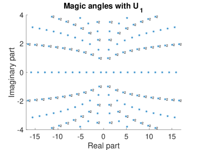
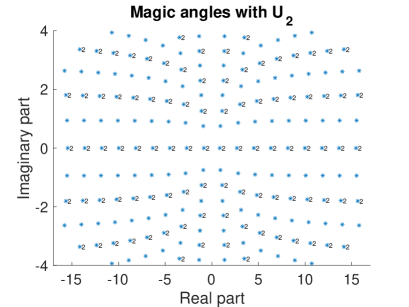
Figure 1. Magic angles $\alpha$ derived from potentials $U=U_{1}$ (left) and $U=U_{2}$ (right) in (1.1). The multiplicity of the flat bands $u$ of $(D(\alpha)+k)u_{k}=0$ is illustrated by the numbers (no number $\rightarrow$ simple magic angle, 2 $\rightarrow$ two-fold degenerate magic angle) in the figure. The movie https://math.berkeley.edu/~zworski/Interpolation.mp4 shows the magic angles for interpolation between these potentials: $U(z)=(\cos\theta-\sin\theta)U_{1}(z)+\sin\theta U_{2}(z)$; multiplicity one magic angles are coded by ${\color[rgb]{1,0,0}*}$ and multiplicity two by ${\color[rgb]{0,0,1}*}$.

$k$		$\alpha_{k}$		$\alpha_{k}-\alpha_{k-1}$
1		0.585663
2		2.221182		1.6355
3		3.751406		1.5302
4		5.276498		1.5251
5		6.794785		1.5183
6		8.312999		1.5182
7		9.829067		1.5161
8		11.345340		1.5163
9		12.860608		1.5153
10		14.376072		1.5155
11		15.890964		1.5149

$k$		$\alpha_{k}$		$\alpha_{k}-\alpha_{k-1}$
1		0.853799
2		2.691433		1.8376
3		4.507960		1.8165
4		6.332311		1.8244
5		8.157130		1.8248
6		9.983510		1.8264
7		11.809376		1.8259
8		13.635446		1.8261
9		15.460894		1.8255
10		17.286231		1.8253
11		19.111041		1.8248

Table 1. First $11$ real magic angles, rounded to 6 digits, for $U=U_{1}$ (left) and $U=U_{2}$ (right). The $\alpha$’s for $U_{1}$ are simple and the ones on the right are double.

Figure 2. Let $\alpha\approx 0.853799$ as in Table 1, lowest two Bloch band with positive energy close to the first magic angle with $U=U_{2}$. We plot $E_{1}(k)$ (left) and $E_{2}(k)$ (right).

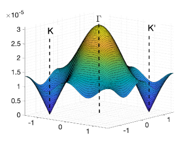
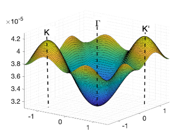
Figure 3. Let $\alpha\approx 0.9628+0.9873i$ the first complex magic angle for $U=U_{1}$, lowest two Bloch band with positive energy close to the first degenerate magic angle. We plot $E_{1}(k)$ (left) and $E_{2}(k)$ (right).

The first theorem is a rigidity result stating that two-fold degenerate $\alpha$’s have to appear in certain representations:

Theorem 1 (Rigidity).

Using (1.5), define $L^{2}_{0,p}:=\{u\in L^{2}_{0}:u(\omega z)=\bar{\omega}^{p}u(z)\}$, $p\in\mathbb{Z}_{3}$. Assume that the Hamiltonian (1.1) satisfies (1.2) and (1.3).

Then, with the definition of multiplicity (1.7) ,

$$\begin{split}&m(\alpha)=1\ \Longrightarrow\ \dim\ker_{L^{2}_{0,2}}D(\alpha)=1,\\ &m(\alpha)=2\ \Longrightarrow\ \dim\ker_{L^{2}_{0,0}}D(\alpha)=\dim\ker_{L^{2}_{0,1}}D(\alpha)=1.\end{split}$$ (1.10)

The first implication in (1.10) is included in [BHZ22b, Theorem 2]. The location of the zeros of the elements of $\ker_{L^{2}_{0,j}}D(\alpha)$ in (1.10) is is described in Theorem 8, see also [BHZ22b, Theorem 3] for the case of simple magic angles.

To prove existence of magic $\alpha$’s of higher multiplicities we use trace computations first used to show that $\mathcal{A}$ is non-empty [Be*22] and then that $|\mathcal{A}|=\infty$ [BHZ22a]. The traces here refer to $\operatorname{tr}T_{k}^{2p}$ where $T_{k}$ is a Birman–Schwinger operator with spectrum given by $\{1/\alpha:\alpha\in\mathcal{A}\}$ - see §2, [Be*22, Theorem 3], [BHZ22a, Theorem 1].

Theorem 1 shows that to show existence of degenerate $\alpha$’s we need to show that $\operatorname{tr}((T_{0}|_{L^{2}_{0,j}})^{2p})\neq 0$, $j=0,1$ (as explained in §3 we are allowed to take $k=0$).

Theorem 2 (Degenerate magic angles).

For the Bistritzer–MacDonald potential, $U_{0}=U_{1}$, defined in (1.8), there exist infinitely many $\alpha\in\mathcal{A}$ which are not simple.

Theorem 7 in §4 states this for for a larger class of potentials satisfying the assumptions of [BHZ22a, Theorem 5] with an additional non-degeneracy condition, see Theorem 6.

It is natural to ask if multiplicities always occur and if multiplicities of higher degree are also ubiquitous. If we do not demand that (1.3) holds, then, generically in the sense of Baire, magic angles are either simple or two-fold degenerate:

Theorem 3 (Generic simplicity).

For Hamiltonians (1.1) satisfying (1.2), there exists a generic subset (an intersection of open dense sets), $\mathscr{V}_{0}\subset\mathscr{V}$, where the space of matrix valued potentials, $\mathscr{V}$, is defined in (6.3), such that if $V\in\mathscr{V}_{0}$ then (see (1.7))

$$m(\alpha)\leq 2.$$

More precisely, when $\alpha$ is simple then

$$\dim\ker_{L^{2}_{0,2}}(D(\alpha))=1\text{ and }\dim\ker_{L^{2}_{0,0}}(D(\alpha))=\dim\ker_{L^{2}_{0,1}}(D(\alpha))=0$$ (1.11)

and when it is double,

$$\dim\ker_{L^{2}_{0,2}}(D(\alpha))=0\text{ and }\dim\ker_{L^{2}_{0,0}}(D(\alpha))=\dim\ker_{L^{2}_{0,1}}(D(\alpha))=1.$$ (1.12)

Remark. It may seem at first the conclusions (1.11),(1.12) follow from Theorem 1. However, in that theorem we assumed also (1.3) which does not need to hold for potentials in $\mathscr{V}_{0}$.

We also have an analogue of [BHZ22b, Theorem 2]: we show that two-fold degenerate flat bands are gapped from the rest of the spectrum.

Theorem 4 (Spectral gap).

Suppose that $D(\alpha)$ is given by (1.1) with $U_{\pm}$ satisfying (1.2). If $\alpha\in\mathcal{A}$ then

$$\begin{split}\forall j>2,&k\in{\mathbb{C}}\quad E_{j}(\alpha,k)>0\ \text{ and }\ E_{1}(\alpha,k)=E_{2}(\alpha,k)=0\\ &\Longleftrightarrow\forall k\in{\mathbb{C}}:\operatorname{dim}\ker_{L^{2}_{0}}(D(\alpha)+k)=2\\ &\Longleftrightarrow\exists p\in{\mathbb{C}}:\operatorname{dim}\ker_{L^{2}_{0}}(D(\alpha)+p)=2.\end{split}$$

The Chern number and Berry curvature associated to the doubly degenerate flat band have similar properties to the case of simple flat bands. In particular, we have the following result proved in 9.

Theorem 5 (Flat band topology).

Let $\alpha\in\mathcal{A}$ be two-fold degenerate. The Chern number of the rank 2 vector bundle $E$ associated to $\ker_{L^{2}_{0}}(D(\alpha)+k)$ (see (9.18)) is

$$c_{1}(E)=-1.$$ (1.13)

In addition, the trace of the curvature, $H$, is non-negative and satisfies $H(k)=H(\omega k)$, $H(k)=H(-k)$.

In Section 10, we collect numerical observations on the possibility of having eigenvalues of $T_{k}$ of algebraic multiplicity $2$ but geometric multiplicity $1$ and thus corresponding to simple magic angles. We also discuss features of the Berry curvature for two-fold degenerate magic angles.

Acknowledgements. We would like to thank Mengxuan Yang for helpful discussions. TH and MZ were partially supported by the National Science Foundation under the grant DMS-1901462 and by the Simons Foundation under a “Moiré Materials Magic” grant.

2. Properties of the Hamiltonian

In this article we will follow the equivalent, but mathematically simpler, notation introduced in [BZ23] and based on the more natural lattice $\Lambda=\omega\mathbb{Z}\oplus\mathbb{Z}$. To do so, we perform the following change of variables $z_{\rm{new}}=\frac{4}{3}\pi z_{\rm{old}}$ - see [BHZ22b, Appendix A].

Thus we work now with (1.1) but now we assume

$$U_{\pm}(z+\gamma)=e^{\pm i\langle\gamma,K\rangle}U_{\pm}(z),\ \ \gamma\in\Lambda,\quad U_{\pm}(\omega z)=\omega U_{\pm}(z).$$ (2.1)

Here and elsewhere, $\langle z,w\rangle:=\operatorname{Re}(z\bar{w})$, $\pm K$ are the nonzero points of high symmetry, $\omega K\equiv K\!\!\mod\!\Lambda^{*}$, $K=\frac{4}{3}\pi$.

The analogue of (1.3) is given by

$$U_{+}(z)=U(z),\ \ \ U_{-}(z)=U(-z),\ \ \ \quad\overline{U(\bar{z})}=-U(-z),$$ (2.2)

and the Bistritzer–MacDonald potential is now $U(z)=-\frac{4}{3}\pi iU_{1}(\frac{4}{3}\pi iz)$, where $U_{1}$ is given in (1.8).

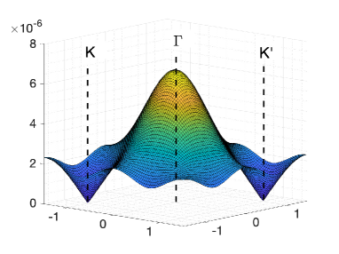
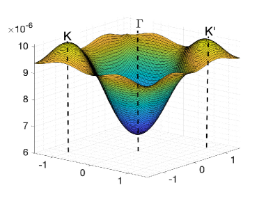
Figure 4. Let $\alpha\approx 0.853799$ as in Table 1, lowest two Bloch band with positive energy close to the first magic angle with $U=U_{2}$. We plot $E_{1}(k)$ (left) and $E_{2}(k)$ (right).

The off-diagonal operator $D(\alpha)$ is

$$D(\alpha)=\begin{pmatrix}2D_{\bar{z}}&\alpha U(z)\\ \alpha U(-z)&2D_{\bar{z}}\end{pmatrix},\quad U(z):=-\tfrac{4}{3}\pi iU_{0}\left(\tfrac{4}{3}\pi iz\right).$$ (2.3)

We then define

$$\rho(z):=\operatorname{diag}(\chi_{k_{j}}(\gamma)),\quad k_{2}=-k_{1}=K,\ \ \in{\mathbb{C}}/\Lambda^{*},\quad\chi_{k}(\gamma):=e^{i\langle\gamma,k\rangle},$$

so that

$$V(z+\gamma)=\rho(\gamma)V(z)\rho(\gamma)^{-1},\ \ \ V(z):=\begin{pmatrix}0&U_{+}(z)\\ U_{-}(z)&0\end{pmatrix}.$$

The modified potential, $V_{\rho}(z):=\rho(z)V(z)\rho(z)^{-1}$, is $\Lambda$-periodic and thus

$$\rho(z)D(\alpha)\rho(z)^{-1}=D_{\rho}(\alpha),\quad D_{\rho}(\alpha):=\operatorname{diag}((2D_{\bar{z}}-k_{j})_{j=1}^{2})+V_{\rho}(z).$$

Using the rotation operator $\Omega u(z)=u(\omega z)$ satisfying $\Omega D(\alpha)=\omega D(\alpha)\Omega$ we can define $\mathscr{C}=\operatorname{diag}(1,\bar{\omega})\Omega$ such that $\mathscr{C}H=H\mathscr{C}$ and translation operator $\mathscr{L}_{\gamma}u(z):=\rho(\gamma)u(z+\gamma).$ By using the translation $\mathscr{L}_{\gamma}$, we can define, for $k\in\mathbb{C}$, the spaces

$$H_{k}^{s}:=H_{k}^{s}({\mathbb{C}}/\Lambda,{\mathbb{C}}^{n}):=\{u\in H^{s}_{\text{loc}}({\mathbb{C}};{\mathbb{C}}^{n}):\mathscr{L}_{\gamma}u=e^{i\langle k,\gamma\rangle}u,\gamma\in\Lambda\},\text{ with }L^{2}_{k}:=H_{k}^{0},$$

where $n=1$ corresponds to the first, $n=2$ to the upper two, and $n=4$ to all components of $\mathscr{L}_{\gamma}.$

When $k\in\mathcal{K}:=\{K,-K,0\}+\Lambda^{*}$ we also define

$$L^{2}_{k,p}=L^{2}_{k,p}(\mathbb{C}/\Gamma;\mathbb{C}^{n}):=\{u\in L^{2}_{k}:u(\omega z)=\bar{\omega}^{p}u(z)\},\ \ L^{2}_{k}=\bigoplus_{p\in{\mathbb{Z}}_{3}}L^{2}_{k,p}.$$

We can then define a generalized Bloch transform

$$\begin{gathered}\mathcal{B}u(z,k):=\sum_{\gamma\in\Lambda}e^{i\langle z+\gamma,k\rangle}\mathscr{L}_{\gamma}u(z),\ \ \ \mathcal{B}u(z,k+p)=e^{i\langle z,p\rangle}\mathcal{B}u(z,k),\ \ p\in\Lambda^{*},\ \ \ u\in\mathscr{S}(\mathbb{C}),\\ \mathscr{L}_{\alpha}\mathcal{B}u(\bullet,k)=\sum_{\gamma}e^{i\langle z+\alpha+\gamma,k\rangle}\mathscr{L}_{\alpha+\gamma}u(z)=\mathcal{B}u(\bullet,k),\ \ \alpha\in\Lambda\end{gathered}$$

such that

$$\begin{gathered}\mathcal{B}D(\alpha)=(D(\alpha)-k)\mathcal{B},\ \ \ D(\alpha)-k=e^{i\langle z,k\rangle}D(\alpha)e^{-i\langle z,k\rangle},\\ \mathcal{B}H(\alpha)=H_{k}(\alpha)\mathcal{B},\ \ \ H_{k}(\alpha):=e^{i\langle z,k\rangle}H(\alpha)e^{-i\langle z,k\rangle}=\begin{pmatrix}\ \ 0&D(\alpha)^{*}-\bar{k}\\ D(\alpha)-k&0\end{pmatrix}.\end{gathered}$$ (2.4)

In particular, we say $H(\alpha)$ exhibits a flat band at energy zero if and only if $0\in\bigcap_{k\in\mathbb{C}}\operatorname{Spec}(H_{k}(\alpha)).$ To study the set of $\alpha$ at which $H(\alpha)$ exhibits a flat band at zero, we define the set of Dirac points $\mathcal{K}_{0}:=\{K,-K\}+\Lambda^{*}$ such that for $k\notin\mathcal{K}_{0}$ we can define the compact Birman-Schwinger operator

$$T_{k}=R(k)V(z):L^{2}_{0}\to L^{2}_{0},\quad R(k)=(2D_{\bar{z}}-k)^{-1}.$$ (2.5)

This operator then characterizes the set of magic angles in the sense stated in the next Proposition

Proposition 2.1 ([Be*22, Theorem 2],[BHZ22b, Proposition 2.2]).

There exists a discrete set $\mathcal{A}$ such that

$$\operatorname{Spec}_{L^{2}_{0}}D(\alpha)=\left\{\begin{array}[]{ll}\mathcal{K}_{0}&\alpha\notin\mathcal{A},\\ \mathbb{C}&\alpha\in\mathcal{A}.\end{array}\right.$$ (2.6)

Moreover,

$$\alpha\in\mathcal{A}\ \Longleftrightarrow\ \exists\,k\notin\mathcal{K}_{0},\ \alpha^{-1}\in\operatorname{Spec}_{L^{2}_{0}}T_{k}\ \Longleftrightarrow\forall\,k\in\mathcal{K}_{0},\alpha^{-1}\in\operatorname{Spec}_{L^{2}_{0}}T_{k},$$ (2.7)

where $T_{k}$ is a compact operator given by

$$T_{k}:=R(k)V(z):L^{2}_{0}\to L^{2}_{0},\ \ \ R(k):=(2D_{\bar{z}}-k)^{-1}$$ (2.8)

In particular, the spectrum of $T_{k_{0}}$ is independent of $k_{0}\notin\mathcal{K}_{0}$ and characterizes parameters $\alpha\in{\mathbb{C}}$ at which the Hamiltonian exhibits a flat band at zero energy. Since the parameter $\alpha$ is inherently connected with the twisting angle, we shall refer to $\alpha$’s at which (2.7) occurs as magic and denote their set by $\mathcal{A}\subset\mathbb{C}$. We then square the operator $T_{k_{0}}^{2}=\operatorname{diag}(A_{k_{0}},B_{k_{0}})$ where $A_{k_{0}}=R(k_{0})U(z)R(k_{0})U(-z).$ Setting $k_{0}=0$, we notice that $T_{0}$ leaves the subspaces $L^{2}_{0,j}$ invariant. By projecting the spaces $L^{2}_{0,j}$ onto the first component, we can define $A_{0}$ on spaces $L^{2}_{0,j}.$

Remark. If $\alpha\in\mathcal{A}$ be simple, then $1/\alpha$ is an eigenvalue of $T_{0}$ with eigenvalue of geometric multiplicity $1$ and the Hamiltonian exhibits a two-fold degenerate flat band at energy zero. If $\alpha\in\mathcal{A}$ is two-fold degenerate, then $1/\alpha$ is an eigenvalue of $T_{0}$ with eigenvalue of geometric multiplicity $2$ and the Hamiltonian exhibits a four-fold degenerate flat band at energy zero. It follows from [BHZ22b, Theorem$2$] and Theorem 4 that we can drop the minima in the above definition.

Suppose that the potential $U(z)$ satisfies the symmetries given in (2.1), namely

$$U(z+\gamma)=e^{i\langle\gamma,K\rangle}U(z),\ \ \ U(\omega z)=\omega U(z).$$

Since $U$ is then periodic with respect to $3\Lambda$ ($3K\equiv 0\!\!\mod\!\Lambda^{*}$), expanding in Fourier series gives

$$U=\sum_{p\in\Lambda^{*}/3}a_{p}e^{i\langle z,p\rangle}$$

. The translational symmetry now writes:

$$\forall p\in\Lambda^{*}/3,\ \ \forall\gamma\in\Lambda,\quad a_{p}e^{i\langle\gamma,p\rangle}=a_{p}e^{i\langle\gamma,K\rangle}.$$

Identifying the Fourier coefficients now gives that for all $p\in\Lambda^{*}/3$,

$$a_{p}\neq 0\ \Longrightarrow\ \forall\,\gamma\in\Lambda,\ \ \langle\gamma,p\rangle=\langle\gamma,K\rangle\ \Longrightarrow\ p\equiv K\!\!\mod\Lambda^{*}.$$

In other words, we see that (changing notation)

$$U(z)=\sum_{p\in\Lambda^{*}}a_{p}e^{i\langle p+K,z\rangle}.$$ (2.9)

We now investigate the rotational symmetry: it is equivalent to

$$\sum_{p\in\Lambda^{*}}a_{p}e^{i\langle\bar{\omega}p+\bar{\omega}K,z\rangle}=f(\omega z)=\omega f(z)=\sum_{p\in\Lambda^{*}}\omega a_{p}e^{i\langle p+K,z\rangle}.$$

Now, $\bar{\omega}p+\bar{\omega}K=\bar{\omega}p-z^{-1}(\omega)+K$, where we defined the rescaling map

$$z:\Lambda^{*}\to\Lambda,\quad z(k):={\sqrt{3}k}/{4\pi i}.$$ (2.10)

Hence, the right hand side of the equality previous equality rewrites

$$f(\omega z)=\sum_{p\in\Lambda^{*}}a_{\omega p+z^{-1}(\bar{\omega})}e^{i\langle p+K,z\rangle},$$

that is $a_{p}=\omega a_{\omega p+z^{-1}(\bar{\omega})}.$ The previous discussion justified the following characterization of potentials $U(z)$ satisfying the symmetries given in (2.1)

$$U(z)\text{ satisfies }\eqref{eq:news}\ \iff\ U(z)=\sum_{p\in\Lambda^{*}}a_{p}e^{i\langle p+K,z\rangle}\text{ and }\forall p\in\Lambda^{*},a_{p}=\omega a_{\omega p+z^{-1}(\bar{\omega})}.$$ (2.11)

In other words, the values of $a_{p}$ are determined on the orbits of

$$\kappa:\Lambda^{*}\in p\mapsto\omega p+z^{-1}(\bar{\omega}),\ \ \ {\rm{Orb}}(p)=\{p,\omega p+z^{-1}(\bar{\omega}),\bar{\omega}p-z^{-1}(\omega)\},\ \ a_{\kappa(p)}=\bar{\omega}a_{p}.$$

So, for instance, the BM potential, up to a factor, comes from the orbit of $p=0$.

In addition there exist a number of further anti-linear symmetries of the chiral Hamiltonian

$$Qv(z)=\overline{v(-z)},\quad\mathscr{Q}u(z)=\begin{pmatrix}0&Q\\ Q&0\end{pmatrix}u(z),$$

satisfying $QD(\alpha)Q=D(\alpha)^{*}$ with $Q:L^{2}_{k,p}({\mathbb{C}}/\Lambda;{\mathbb{C}}^{2})\to L^{2}_{k,-p}({\mathbb{C}}/\Lambda;{\mathbb{C}}^{2})$ with $\mathscr{Q}:L^{2}_{k,p}({\mathbb{C}}/\Lambda;{\mathbb{C}}^{4})\to L^{2}_{k,-p+1}({\mathbb{C}}/\Lambda;{\mathbb{C}}^{4})$ satisfying $H(\alpha)\mathscr{Q}=\mathscr{Q}H(\alpha)$ and

$$\mathscr{E}v(z):=Jv(-z),\quad J:=\begin{pmatrix}0&1\\ -1&0\end{pmatrix}$$

with $\mathscr{E}:L^{2}_{\pm K,\ell}({\mathbb{C}}/\Lambda;{\mathbb{C}}^{2})\to L^{2}_{\mp K,\ell}({\mathbb{C}}/\Lambda;{\mathbb{C}}^{2})$ and

$$\mathscr{E}:L^{2}_{0,\ell}({\mathbb{C}}/\Lambda;{\mathbb{C}}^{2})\to L^{2}_{0,\ell}({\mathbb{C}}/\Lambda;{\mathbb{C}}^{2})\text{ satisfying }\mathscr{E}D(\alpha)\mathscr{E}^{*}=-D(\alpha).$$ (2.12)

Finally, we also introduce their composition $\mathscr{A}:L^{2}_{k,p}({\mathbb{C}}/\Lambda;{\mathbb{C}}^{2})\to L^{2}_{k,-p}({\mathbb{C}}/\Lambda;{\mathbb{C}}^{2})$

$$\mathscr{A}:=\mathscr{E}Q,\text{ with }\mathscr{A}v(z):=\begin{pmatrix}0&1\\ -1&0\end{pmatrix}\overline{v(z)}$$ (2.13)

with $\mathscr{A}D(\alpha)\mathscr{A}=-D(\alpha)^{*}.$

Using the above symmetries, we observe that

Proposition 2.2.

The spectrum of $RV$ satisfies $\operatorname{Spec}_{L^{2}_{0,p}}(RV)=\operatorname{Spec}_{L^{2}_{0,-p+1}}(RV).$ In particular, for $m\geq 2$ we find $\operatorname{tr}_{L^{2}_{0,p}}(RV)^{2m}=\operatorname{tr}_{L^{2}_{0,-p+1}}(RV)^{2m}.$

Proof.

Let $v\in L^{2}_{0,p}$ satisfy $RVv=-\lambda v$ then by multiplying by $2D_{\bar{z}}$ we find $D(1/\lambda)v=0$. Thus, $D(1/\lambda)^{*}Qv=0$ with $Qv\in L^{2}_{0,-p}.$ We thus have

$$0=D(1/\lambda)^{*}Qv=D(1/\lambda)^{*}R^{*}(2D_{z})Qv.$$

We conclude that $(2D_{z})Qv\in L^{2}_{0,-p+1}$ is an eigenvector to $(RV)^{*}$ with eigenvalue $-\bar{\lambda}.$ ∎

3. Trace computations

To prove the existence of degenerate magic angles (Theorem 2) we argue by contradiction using the Birman–Schwinger operator $T_{k}$ defined in (2.5). From theorem 1, we see that in the case if all the $\alpha$’s were all simple then the traces of $T_{k}^{2p}$ restricted to $L^{2}_{0,0}$ or $L^{2}_{0,1}$ would have to vanish. For a general $k$, the operator $T_{k}$ does not preserve the rotational invariant subspaces $L^{2}_{0,j}$. To achieve that we set $k=0$ so that the proof reduces to showing that $\operatorname{tr}((T_{0})_{L^{2}_{0,0}}^{2\ell})\neq 0$ for some value of $\ell$. That is done using the previous rationality condition $\operatorname{tr}((T_{0})_{L^{2}_{0,0}}^{2\ell})=q_{\ell}\pi/\sqrt{3}$ for $q_{\ell}\in\mathbb{Q}$ obtained before by the authors [BHZ22a][Theorem 1] and some elementary arguments involving transcendental numbers.

3.1. Traces on rotationally invariant subspaces

We recall that an orthonormal basis of $L_{0}^{2}(\mathbb{C}/3\Lambda;\mathbb{C})$ is given by setting

$$e_{\nu}(z):=e^{i\langle\nu,z\rangle}/\sqrt{\mathrm{Vol}(\mathbb{C}/3\Lambda)},\quad\nu\in\Lambda^{*}+K,\ \ \langle\nu,z\rangle:=\mathrm{Re}(\bar{z}\nu).$$

We see that $\Omega e_{\nu}=e_{\bar{\omega}\nu}.$ This means that an orthonormal basis of $L^{2}_{{0,j}}$ is given by

$$e_{[\nu]}(z)=\frac{1}{\sqrt{3}}\big{(}e_{\nu}(z)+\omega^{j}e_{\omega\nu}(z)+\bar{\omega}^{j}e_{\bar{\omega}\nu}(z)\big{)},\;\;\nu\in\Lambda^{*}+K,\;\;[\nu]=\{\nu,\omega\nu,\bar{\omega}\nu\}.$$

Following our approach developed in [BHZ22a], we compute the sum of powers of magic angles by computing traces of the operator $T_{k}$ defined in (2.8). Since odd powers of $T_{k}$ have vanishing traces it suffices to compute the traces of powers of the Hilbert-Schmidt operator

$$A_{k}:=R(k)U(z)R(k)U(-z):L^{2}_{0}\to L^{2}_{0},\quad k\notin(K+\Lambda^{*})\cup(-K+\Lambda^{*})=\mathcal{K}_{0}.$$ (3.1)

Due to the relation

$$\forall k\notin\mathcal{K}_{0},\quad\Omega^{-1}A_{k}\Omega=A_{\omega k},$$

we see that subspaces $L^{2}_{0,j}$ are not in general invariant by $A_{k}$. This makes a direct application of the strategy of [BHZ22a] impossible. However, we see that the operator $A_{0}$ does preserve this smaller subspace. From now on, we therefore specialize to $k=0$. For $\ell\geq 2$, one can compute the trace on $L^{2}_{{0,j}}$:

$$\operatorname{tr}\big{(}(A_{0})^{\ell}_{|L^{2}_{{0,j}}}\big{)}=\sum_{[\nu],\nu\in\Lambda^{*}+K}\langle A_{0}^{\ell}e_{[\nu]},e_{[\nu]}\rangle.$$

Now, we write that, using bilinearity of the scalar product

$$3\langle A_{0}^{\ell}e_{[\nu]},e_{[\nu]}\rangle=\sum_{h=0}^{2}\langle A_{0}^{\ell}e_{\omega^{h}\nu},e_{\omega^{h}\nu}\rangle+\sum_{k\neq h}\omega^{j(k-h)}\langle A_{0}^{\ell}e_{\omega^{h}\nu},e_{\omega^{k}\nu}\rangle.$$

Thus, when summing on $[\nu]$, the first term gives a third of the trace on $L^{2}_{0}$, (which was computed in [Be*22] for $\ell=2$ and $U_{0}=U_{1}$ and shown to be equal to $4\pi/\sqrt{3}$)

$$\begin{split}\operatorname{tr}((A_{0})^{\ell}_{|L^{2}_{{0,j}}})&=\tfrac{1}{3}\operatorname{tr}(A_{0}^{\ell})+\tfrac{1}{3}\sum_{[\nu],\nu\in\Lambda^{*}+K}\sum_{k\neq h}\omega^{j(k-h)}\langle A_{0}^{\ell}e_{\omega^{h}\nu},e_{\omega^{k}\nu}\rangle\\ &=:\tfrac{1}{3}\operatorname{tr}(A_{0}^{2})+\tfrac{1}{3}\mathcal{R}_{\ell,j}.\end{split}$$ (3.2)

3.2. Existence of degenerate magic angles

Our strategy now consists in using [BHZ22a, Theorem1] and the fact that $\pi/\sqrt{3}$ is transcendental to contradict the conclusion of theorem 1. More explicitly, we will prove the following statement:

Theorem 6.

Let $U\in C^{\infty}(\mathbb{C}/3\Lambda)$ satisfying the first two symmetries of (2.1) with only finitely many non-zero Fourier modes $a_{p}\in\pi\mathbb{Q}(\omega/\sqrt{3})$, appearing in the decomposition (2.11). Then, if we denote $\mathcal{A}(U)$ the set of $($complex$)$ magic angles for the potential $U$ and if $\mathcal{A}(U)\neq\emptyset$, there exists $\alpha \in\mathcal{A}(U)$ which is not simple. This is, in particular true for the the Bistritzer–MacDonald potential $U_{1}$ defined in (1.8).

Proof.

We start by noticing that the existence of a magic angle is equivalent to the existence of a non-vanishing trace

$$\exists\ell\geq 2,\quad\operatorname{tr}((A_{0})_{|L^{2}_{0}}^{\ell})\neq 0.$$

This follows from the properties of the regularized Fredholm determinant, cf. [BHZ22a]. We fix such an $\ell$. Using [BHZ22a, Theorem $5$], and the hypothesis on the potential, this implies that $\operatorname{tr}(A_{0}^{\ell})\in\pi\mathbb{Q}(\omega)$. Since the trace is non-zero by assumption, this proves that $\operatorname{tr}(A_{0}^{\ell})$ is transcendental. The idea is to prove that the sum defining the remainder $\mathcal{R}_{\ell,j}$ is always a finite sum, under the assumption that the potential has only finitely many non-zero Fourier mode. We then prove that, by assuming that $a_{p}\in\pi\mathbb{Q}(\omega/\sqrt{3})$, each term in the sum defining $\mathcal{R}_{\ell,j}$ is in $\mathbb{Q}(\omega)$ so that $\mathcal{R}_{\ell,j}\in\mathbb{Q}(\omega)$ is algebraic. This will prove that $\operatorname{tr}((A_{0})^{\ell}_{|L^{2}_{{0,j}}})\neq 0$ by (3.2) and contradict the conclusion of theorem 1; thus proving the existence of non-simple magic angle for the potential $U$. We start with the formula defining the remainder

$$\mathcal{R}_{\ell,j}:=\sum_{[\nu],\nu\in\Lambda^{*}+K}\sum_{k\neq h}\omega^{j(k-h)}\langle A_{0}^{\ell}e_{\omega^{h}\nu},e_{\omega^{k}\nu}\rangle.$$

The summand $\langle A_{0}^{\ell}e_{\omega^{h}\nu},e_{\omega^{k}\nu}\rangle$ is non-zero only if $A_{0}^{\ell}e_{\omega^{h}\nu}$ has a non-vanishing Fourier mode corresponding to $e_{\omega^{k}\nu}$. Now, if we look at the definition of $A_{0}$ (see 3.1), we see that the $R(k)$ part acts diagonally (with coefficients in $(i\pi)^{-1}\mathbb{Q}(\omega)$ as we chose $k=0$) on the Fourier basis, on the other hand, the $U(z)$ and $U(-z)$ parts act as a finite sum of weighted shifts on this basis (it is here where we use the assumption of having finitely many non-vanishing Fourier modes). Moreover, by assumption, the weights are elements of $(i\pi)\mathbb{Q}(\omega)$.This means that there exists a finite subset $\mathcal{F}_{U}^{\ell}\subset 3\Gamma^{*}$ such that

$$\forall\nu\in\Lambda^{*}+K,\quad A_{0}^{\ell}e_{\nu}=\sum_{\eta\in\mathcal{F}_{U}^{\ell}}a_{\eta}e_{\nu+\eta},\quad a_{\eta}\in\mathbb{Q}(\omega).$$ (3.3)

But this means that there exists a constant $R>0$ such that for any $\eta\in\mathcal{F}_{U}^{\ell}$, we have $|\eta|\leq R$. In particular, if $\langle A_{0}^{\ell}e_{\omega^{h}\nu},e_{\omega^{k}\nu}\rangle$ is non-zero, then $|\omega^{h}\nu-\omega^{k}\nu|\leq R$. Now, because $h\neq j$, this inequality is false outside a compact set for $\nu$. But because $\nu$ is on a lattice, which is discrete, we conclude that the above inequality is true for at most a finite number of $\nu$. Thus, the sum defining $\mathcal{R}_{\ell,j}$ is finite.
Finally, for the non-zero terms of the sum, we use (3.3) again to conclude that $\langle A_{0}^{\ell}e_{\omega^{h}\nu},e_{\omega^{k}\nu}\rangle=a_{\eta}\in\mathbb{Q}(\omega).$ This proves the existence of a non-simple magic angle for the potential $U$. ∎

4. Infinite number of degenerate magic angles

We now adapt the argument, already used in [BHZ22a, Theorem $6$], to prove that the number of non-simple magic angles is actually infinite. This actually refines the previous theorem by showing there is an infinite number of non-simple magic angles.

In the next theorem we use the same notation and assumptions as in Theorem 6. The definition of multiplicity is given in (1.9).

Theorem 7.

Let

$$\mathcal{A}_{m}(U):=\{\alpha\in\mathcal{A}(U):m_{U}(\alpha)\geq 2\}$$

be the set of non-simple magic angles. Then

$$|\mathcal{A}(U)|>0\ \Longrightarrow\ |\mathcal{A}_{m}(U)|=+\infty.$$ (4.1)

In particular, the set of magic angles for the Bistritzer–MacDonald potential $U=U_{1}$ (see (1.8)) is infinite.

In addition, if for $N\geq 0$, and $a=(a_{p})_{\{p\in\Lambda^{*};\|p\|_{\infty}\leq N\}}$, $U_{a}$ is given by (2.11) with coefficients $a$, then (4.1) holds for a generic $($in the sense of Baire$)$ set of coefficients $a=(a_{p})_{\{p\in\Lambda^{*};\|p\|_{\infty}\leq N\}}\in\mathbb{C}^{(2N+1)^{2}}$ which contains $(\pi\mathbb{Q}(\omega/\sqrt{3}))^{(2N+1)^{2}}.$ Here, we used the notation $\|p\|_{\infty}=\|\tfrac{4\pi i}{\sqrt{3}}(p_{1}+p_{2}\omega)\|_{\infty}:=\max(p_{1},p_{2}).$

Proof.

We start by observing that since $\pi$ is transcendental on $\mathbb{Q}$, it is also transcendental in $\mathbb{Q}(\omega/\sqrt{3}).$ Now, we shall assume that there exist only finitely many non-simple eigenvalues of $A_{0}^{2}$ on $L^{2}_{0}$. This implies, by theorem 1 that $(A_{0})^{\ell}_{|L^{2}_{{0,1}}}$ has only finitely many eigenvalues, we denote them by $\lambda_{i}\in\mathbb{C}$ for $i=1,..,N$. Then we define the $n$-th symmetric polynomial

$$e_{n}(\lambda_{1},\ldots,\lambda_{N})=\sum_{1\leq j_{1}<j_{2}<\cdots<j_{n}\leq N}\lambda_{j_{1}}\dotsm\lambda_{j_{n}}.$$

Newton identities show that this polynomial can be expressed as

$$e_{n}(\lambda_{1},\ldots,\lambda_{N})=(-1)^{n}\sum_{m_{1}+2m_{2}+\cdots+nm_{n}=n\atop m_{1}\geq 0,\ldots,m_{n}\geq 0}\prod_{i=1}^{n}\frac{(-\operatorname{tr}(A_{0})^{2i}_{|L^{2}_{{0,1}}})^{m_{i}}}{m_{i}!i^{m_{i}}}$$ (4.2)

where $e_{n}=0$ for $n>N.$ The fact that $\mathcal{A}(U)\neq\emptyset$ implies, by theorem 6 that $\mathcal{A}_{m}(U)\neq\emptyset$. Now, this means that there is a non-vanishing trace of $(A_{0})^{\ell}_{|L^{2}_{{0,2}}}$. Choose $m_{0}$ to be the minimal power for which the trace is non-zero. Choose $n=m_{0}\times K$ where $K$ is a large integer, and using the fact that $e_{n}=0$, we deduce that $\pi$ is the root of the polynomial of degree $K$ with coefficients in $\mathbb{Q}\left(\frac{\omega}{\sqrt{3}}\right)$ given by

$$\begin{split}\sum_{m_{1}+2m_{2}+\cdots+nm_{n}=n\atop m_{1}\geq 0,\ldots,m_{n}\geq 0}\prod_{i=1}^{m_{0}\times K}(\operatorname{tr}(A_{0})^{2i}_{|L^{2}_{{0,1}}})^{m_{i}}&=\sum_{m_{1}+2m_{2}+\cdots+nm_{n}=n\atop m_{1}\geq 0,\ldots,m_{n}\geq 0}\prod_{i=1}^{m_{0}\times K}(\underbrace{\frac{1}{3}\operatorname{tr}(A_{0})^{2i}_{|L^{2}_{{0}}}}_{\in\mathbb{Q}\left(\frac{\omega}{\sqrt{3}}\right)\pi}-\underbrace{\mathcal{R}_{i,1}}_{\in\mathbb{Q}\left(\frac{\omega}{\sqrt{3}}\right)})^{m_{i}}\\ &=0.\end{split}$$

The power $m_{1}\cdots m_{n}$ of $\pi$ is maximized, among the tuples we sum by the unique choice $m_{i}=\delta_{i,m_{0}}K$. By choice of $m_{0}$, this gives that the above polynomial has a non-zero leading coefficient and is therefore non-zero. This contradicts the fact that $\pi$ is transcendental and concludes the proof.

Now, let $a=(a_{p})_{\{p\in\Lambda^{*};\|p\|_{\infty}\leq N\}}\in\mathbb{C}^{(2N+1)^{2}}\in\mathbb{C}^{(2N+1)^{2}}$ and assume that $\mathcal{A}(U_{a})\neq\emptyset$. Then, we can find an open neighborhood of $a$, $\Omega_{a}\ni a$, such that for coefficients $b=(b_{p})_{\{p\in\Lambda^{*};\|p\|_{\infty}\leq N\}}\in\Omega_{a}$ we have $\mathcal{A}(U_{b})\neq\emptyset$. Take $q=(q_{p})_{\{p\in\Lambda^{*};\|p\|_{\infty}\leq N\}}\in(\pi\mathbb{Q}(\omega/\sqrt{3}))^{(2N+1)^{2}}\cap\Omega_{a}$ for which we then have $|\mathcal{A}(U_{q})|=\infty.$ Continuity of eigenvalues of $T_{k}$ as the potential $U$ changes shows that the $V_{m,a}:=\{b\in\Omega_{a}:|\mathcal{A}(U_{b})|\geq m\}$ is open and dense in $\Omega_{a}$. Hence, the set coefficients for which $0<|\mathcal{A}(U_{b})|<\infty$ is given by $\bigcup_{m\in\mathbb{N}}\bigcup_{q\in(\mathbb{Q}+i\mathbb{Q})^{2N+1}}\Omega_{q}\setminus V_{m,q}$. It is then meagre and does not contain $(\pi\mathbb{Q}(\omega/\sqrt{3}))^{(2N+1)^{2}}.$ ∎

5. Numerical evaluation of the trace and existence of non-real magic angle

In this section the potential $U$ will be taken to be equal to $U_{1}$ defined in (1.8). In the last section, we have proven that the traces on the rotational-invariant subspaces can be written as

$$\operatorname{tr}((A_{0})^{\ell}_{|L^{2}_{{0,j}}})=\tfrac{1}{3}\operatorname{tr}(A_{0}^{\ell})+\tfrac{1}{3}\mathcal{R}_{\ell,j},$$ (5.1)

where the remainder was shown to be a finite sum. Although the first term $\operatorname{tr}(A_{0}^{\ell})$ is a priori an infinite sum, the authors provided in [BHZ22a, Theo. 7] a semi-explicit formula which can be evaluated rigorously with computer assistance for $U=U_{1}$ and small values of $\ell$. From [BHZ22a, Table 1], we see that

$$\operatorname{tr}((A_{0}^{2})_{|L^{2}_{0}})=\frac{4\pi}{\sqrt{3}},\quad\operatorname{tr}((A_{0}^{3})_{|L^{2}_{0}})=\frac{96\pi}{7\sqrt{3}},\quad\operatorname{tr}((A_{0}^{4})_{|L^{2}_{0}})=\frac{40\pi}{\sqrt{3}}.$$

We can read off from the above $\operatorname{tr}(A_{0}^{2})\operatorname{tr}(A_{0}^{4})<\operatorname{tr}(A_{0}^{3})^{2}$. If all magic angles were real, then by $\ell^{p}$-interpolation $\operatorname{tr}(A_{0}^{2})\operatorname{tr}(A_{0}^{4})\geq\operatorname{tr}(A_{0}^{3})^{2}$, which is a contradiction. In other words, we have proven that

Proposition 5.1.

Let $U=U_{1}$ be the potential defined in (1.8), then $\mathcal{A}\cap{\mathbb{C}}\setminus{\mathbb{R}}\neq\emptyset.$

Our goal here is to mimic this argument on rotational-invariant subspace by computing the finite remainders $\mathcal{R}_{\ell,j}$ using computer assistance to find the exact results.

From doing so, we obtain the following result.

Proposition 5.2.

For the Bistritzer-MacDonald potential $U_{1}$ defined in (1.8), we have

$$\operatorname{tr}((A_{0}^{2})_{|L^{2}_{0,1}})=\operatorname{tr}((A_{0}^{2})_{|L^{2}_{0,0}})=\frac{4\pi}{3\sqrt{3}}-3\approx-0.581601<0$$

and $\operatorname{tr}((A_{0}^{2})_{|L^{2}_{0,2}})=\frac{4\pi}{\sqrt{3}}+6\approx 8.4184.$ For the higher powers, we find

$$\operatorname{tr}((A_{0}^{3})_{|L^{2}_{0,2}})=\frac{32\pi}{7\sqrt{3}}+\frac{810}{49}\approx 24.8223\text{ and }\operatorname{tr}((A_{0}^{4})_{|L^{2}_{0,2}})=\frac{40\pi}{3\sqrt{3}}+\frac{4374}{91}\approx 72.2499.$$

This implies the inequality

$$\operatorname{tr}((A_{0}^{2})_{|L^{2}_{0,2}})\operatorname{tr}((A_{0}^{4})_{|L^{2}_{0,2}})<\operatorname{tr}((A_{0}^{3})_{|L^{2}_{0,2}})^{2}.$$

We conclude that for any $j\in\mathbb{Z}_{3}$, there is a non-real magic angle $\alpha_{j}\in{\mathbb{C}}\setminus{\mathbb{R}}$ with corresponding eigenfunction $u\in L^{2}_{0,j}$ of $T_{k}$. By Theorem 1, we conclude the existence of non-real and non-simple magic angles.

We note that as the traces depend continuously on the potential $U$, the inequalities

$$\operatorname{tr}((A_{0}^{2})_{|L^{2}_{0,1}})=\operatorname{tr}((A_{0}^{2})_{|L^{2}_{0,0}})<0\text{ and }\operatorname{tr}((A_{0}^{2})_{|L^{2}_{0,2}})\operatorname{tr}((A_{0}^{4})_{|L^{2}_{0,2}})<\operatorname{tr}((A_{0}^{3})_{|L^{2}_{0,2}})^{2}$$

remain true for small perturbations of $U$ and so does the existence of a non-real and non-simple magic angle. As stated in the introduction, the potential $U_{2}$, defined in (1.8), leads to real and doubly-degenerate magic angles. We then see numerically that $\operatorname{tr}((A_{0}^{2})_{|L^{2}_{0,1}})=\operatorname{tr}((A_{0}^{2})_{|L^{2}_{0,0}})>0$, see Figure 5. To interpolate between these two opposite behaviors, we introduce the potentials

$$U_{\theta}(z):=U(z)=(\cos\theta-\sin\theta)U_{1}(z)+\sin\theta U_{2}(z),$$ (5.2)

see https://math.berkeley.edu/~zworski/Interpolation.mp4 for a movie showing the dependence of the set of magic angle when $\theta$ varies.

In Figure 5 we show $\operatorname{tr}((A_{0}^{2})_{|L^{2}_{0,0}}),\operatorname{tr}((A_{0}^{2})_{|L^{2}_{0,2}})$ as a function of $\theta$, verifying that the inequality $\operatorname{tr}((A_{0}^{2})_{|L^{2}_{0,0}})<0$ holds for a large range of values $\theta$.

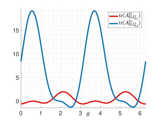
Figure 5. ${\color[rgb]{1,0,0}\operatorname{tr}((A_{0}^{2})_{|L^{2}_{0,1}})}$ and ${\color[rgb]{0,0,1}\operatorname{tr}((A_{0}^{2})_{|L^{2}_{0,2}})}$ for potentials $U_{\theta}(z)$ in (5.2). While for $\theta=0$, $U_{\theta=0}=U_{1}$ we see that $\operatorname{tr}((A_{0}^{2})_{|L^{2}_{0,2}})>0$ and $\operatorname{tr}((A_{0}^{2})_{|L^{2}_{0,1}})<0$. For $\theta=2\pi 7/8\approx 5.5$ and $U_{\theta=2\pi 7/8}=U_{2}$ we have $\operatorname{tr}((A_{0}^{2})_{|L^{2}_{0,2}})<0$ and $\operatorname{tr}((A_{0}^{2})_{|L^{2}_{0,1}})>0$, instead.

Remark. This previous computation could be made rigorous at the cost of adapting the algorithm used in [BHZ22a, Theo. 7] to the potential $U_{\theta}$ in order to compute the first term in (5.1).

6. Generic simplicity in each representation

6.1. Generalized potentials

We now consider the general class of potentials $U_{\pm}(z)$ satisfying

$$U_{\pm}(\omega z)=\omega U_{\pm}(z),U_{\pm}(z+\gamma)=e^{\mp 2i\langle\gamma,K\rangle}U_{\pm}(z),\quad\gamma\in\Gamma.$$ (6.1)

We do not however assume $\overline{U_{\pm}(\bar{z})}=-U_{\pm}(z)$ and then define

$$V(z):=\begin{pmatrix}0&U_{+}(z)\\ U_{-}(z)&0\end{pmatrix}\text{ such that }D_{V}(\alpha)=2D_{\bar{z}}+\alpha V(z).$$

It is convenient to use the following Hilbert space of real analytic potentials defined using the following norm: for fixed $\delta>0$,

$$\|V\|_{\delta}^{2}:=\sum_{\pm}\sum_{k\in\Lambda^{*}/3}|a^{\pm}_{k}|^{2}e^{2|k|\delta},\ \ \ \ U_{\pm}(z)=\sum_{k\in K+\Lambda^{*}}a^{\pm}_{k}e^{\pm i\langle z,k\rangle}.$$ (6.2)

Then we define $\mathscr{V}=\mathscr{V}_{\delta}$ by

$$V\in\mathscr{V}\ \Longleftrightarrow\ \text{ $V$ satisfies \eqref{eq:newU}, }\ \|V\|_{\delta}<\infty.$$ (6.3)

We note that we have as before,

$$\mathscr{L}_{\mathbf{a}}D_{V}(\alpha)=D_{V}(\alpha)\mathscr{L}_{\mathbf{a}},\ \ \ \Omega D_{V}(\alpha)=D_{V}(\alpha)\Omega.$$

We also recall the antilinear symmetry $\mathscr{A}:L^{2}_{k,j}\to L^{2}_{k,-j}$ defined by

$$\mathscr{A}:=\begin{pmatrix}\ \ 0&\Gamma\\ -\Gamma&0\end{pmatrix},\ \ \Gamma v(z)=\overline{v(z)},\ \ \ \ \mathscr{A}D_{V}(\alpha)\mathscr{A}={-}D_{V}(\alpha)^{*}.$$ (6.4)

6.2. Proof of generic simplicity

Our proof of Theorem 3 is an adaptation of the argument for generic simplicity of resonances by Klopp–Zworski [KZ95] – see also [DyZw19, §4.5.5].

We then use the decomposition

$$L^{2}_{0}=\bigoplus_{j=0}^{2}L^{2}_{{0,j}},\ \ \ L^{2}_{{0,j}}\simeq L^{2}(F),$$

where $F$ is a fixed fundamental domain of $G_{3}$. For $V\in\mathscr{V}$ and $R=(2D_{\bar{z}})^{-1}$

$$V:L^{2}_{{0,j}}\to L^{2}_{{0,j-1}},\ \ \ R:L^{2}_{0,j-1}\to L^{2}_{0,j}\ \Longrightarrow\ RV:L^{2}_{0,j}\to L^{2}_{0,j}.$$

Before proceeding we record the following regularity result:

Lemma 6.1.

Suppose that for some $\lambda\in\mathbb{C}$ and $k\in\mathbb{N}$ and $w\in L^{2}(\mathbb{C}/3\Lambda;\mathbb{C})$, $(RV-\lambda)^{k}w=0$. Then $w\in C^{\omega}(\mathbb{C}/3\Lambda;\mathbb{C})$, that is, $w$ is real analytic. The same conclusion holds if $(V^{*}R^{*}-\lambda)^{k}w=0$.

Proof.

We prove a slightly more general statement that $(RV-\lambda)^{k}w=f\in C^{\omega}(\mathbb{C}/3\Lambda;\mathbb{C}^{2})$ implies that $w\in C^{\omega}(\mathbb{C}/3\Lambda;\mathbb{C}^{2})$. We proceed by induction on $k$. For $k=0$, $w=f$. If $k>0$, we put $\widetilde{w}:=(RV-\lambda)^{k-1}{w}$ and note that (the case of $\lambda=0$ is even simpler)

$$D_{V}(-1/\lambda)\widetilde{w}=2\lambda^{-1}D_{\bar{z}}(RV-\lambda)\widetilde{w}=2\lambda^{-1}D_{\bar{z}}{f}\in C^{\omega}.$$

This means that $\widetilde{w}$ is a solution of an elliptic equation with analytic coefficients, hence it is analytic [HöI, Theorem 9.5.1]. The inductive hypothesis now shows that $w$ is analytic.

In the case of $(V^{*}R^{*}-\lambda)^{k}{w}=0$, we proceed similarly but put $\widetilde{w}:=R^{*}(V^{*}R^{*}-\lambda)^{k-1}{w}$, so that

$$D_{V}(-1/\bar{\lambda})^{*}\widetilde{w}=2\bar{\lambda}^{-1}D_{z}R^{*}(V^{*}R^{*}-\lambda)(V^{*}R^{*}-\lambda)^{k-1}{w}=2\bar{\lambda}^{-1}D_{z}R^{*}{f}\in C^{\omega}.$$

Since $(V^{*}R^{*}-\lambda)^{k-1}w=2D_{z}\widetilde{w}$ the inductive argument proceeds as before. ∎

The next lemma shows that we have generic simplicity for operators restricted to the three representations:

Lemma 6.2.

There exists a generic subset of $\mathscr{V}_{j}$ of $\mathscr{V}$ such that for $V\in\mathscr{V}_{j}$, the eigenvalues of $RV|_{L^{2}_{0,j}}$ are simple.

Proof.

We follow the presentation in the proof of [DyZw19, Theorem 4.39] with modifications needed for our case. We fix $j$ and consider all operators as acting on $\mathscr{H}:=L^{2}_{{0,j}}$. The eigenvalue multiplicity is defined using the resolvent:

$$m_{V}(\lambda):=\frac{1}{2\pi i}\operatorname{tr}\oint_{\lambda}(\zeta-RV)^{-1}d\zeta,$$

where the integral is over a sufficiently small positively oriented circle around $\lambda$. We then define

$$\mathscr{E}_{r}:=\{W\in\mathscr{V}:m_{W}(\lambda)\leq 1,\ \lambda\in\mathbb{C}\setminus D(0,r)\}.$$ (6.5)

We want to show that for $r>0$, $\mathscr{E}_{r}$ is open and dense. That will show that the set

$$\mathscr{E}:=\{W\in\mathscr{V}:\ \forall\,\lambda,\ m_{W}(\lambda)\leq 1\}=\bigcap_{n\in{\mathbb{N}}}\mathscr{E}_{\frac{1}{n}}$$

is generic (and in particular, by the Baire category theorem, it has a nowhere dense complement).

Suppose that $RW$ has exactly one eigenvalue $\lambda_{0}$ in $D(\lambda,r)$ and $\operatorname{Spec}(RW)\cap D(\lambda,2r)=\{\lambda_{0}\}$. Putting $\Omega:=D(\lambda,r)$ we then define

$$\Pi_{W}(\Omega):=\frac{1}{2\pi i}\int_{\partial\Omega}(\zeta-RW)^{-1}d\zeta,\ \ \ m_{W}(\Omega):=\operatorname{tr}\Pi_{W}(\Omega).$$ (6.6)

If $V\in\mathscr{V}$ and $\|V\|_{\delta}$ is sufficiently small then for $\zeta\in\partial\Omega$,

$$(R(W+V)-\zeta)^{-1}=(RW-\zeta)^{-1}(I+RV(RW-\zeta)^{-1})^{-1},$$

exists and we can define $\Pi_{W+{V}}(\Omega)$ as in (6.6). This also shows that if $\|{V}\|_{\delta}<\varepsilon$ for sufficiently small $\varepsilon$ then for $\zeta\in\partial\Omega$,

$$(RW-\zeta)^{-1}-(R(W+{V})-\zeta)^{-1}=\mathcal{O}_{\varepsilon}(\|{V}\|_{\delta})_{\mathscr{H}\to\mathscr{H}}.$$

It follows that $\|\Pi_{W}(\Omega)-\Pi_{W+{V}}(\Omega)\|_{\mathscr{H}\to\mathscr{H}}\leq C_{\varepsilon}\|{V}\|_{\delta}$. In particular, if we take $\|{V}\|_{\delta}<1/C_{\varepsilon}$, then $\Pi_{W}(\Omega)$ and $\Pi_{W+{V}}(\Omega)$ have the same rank

$$m_{W+V}(\Omega) \|V\|_{\delta}$$ is constant for sufficiently small. (6.7)

This immediately implies that $\mathscr{E}_{r}$ is open: if $\lambda$ is a simple eigenvalue of $RW$ then $m_{W}(\Omega)=1$ this values does not change under small perturbations.

Now we want to show that $\mathscr{E}_{r}$ is dense. This follows from the following statement

$$\begin{gathered}\forall\;W\in\mathscr{V},\ \varepsilon>0\ \ \exists\;V\in\mathscr{V}\ \ \ W+V\in\mathscr{E}_{r},\ \ \ \ \|V\|_{\delta}<\varepsilon.\end{gathered}$$ (6.8)

As the number of eigenvalues of $RW$ outside $D(0,r)$ is finite, it is enough to prove a local statement as it can be applied successively to obtain (6.8) (once an eigenvalue is simple it stays simple for sufficiently small perturbations). That is, it is enough to show that

$$\begin{gathered}\forall\;W\in\mathscr{V},\ \varepsilon>0\ \ \exists\;V\in\mathscr{V}\ \forall\,\lambda\in\Omega\\ m_{W+V}(\lambda)\leq 1,\ \ \ \|V\|_{\delta}<\varepsilon.\end{gathered}$$ (6.9)

As in [KZ95] we proceed by induction and start by noting that one of two cases has to occur:

$$\begin{gathered}\forall\,\varepsilon>0\ \ \exists\,V\in\mathscr{V},\ \lambda\in\Omega\ \ \ 1\leq m_{W+V}(\lambda)<m_{W+V}(\Omega),\ \ \ \|V\|_{\delta}<\varepsilon,\end{gathered}$$ (6.10)

or

$$\begin{gathered}\exists\,\varepsilon>0\ \forall\,V\in\mathscr{V},\|V\|_{\delta}<\varepsilon\ \exists\,\lambda=\lambda(V)\in\Omega\ \ \ m_{W+V}(\lambda)=m_{W+V}(\Omega).\end{gathered}$$ (6.11)

The first case implies that adding an arbitrarily small $V$ to $W$ produces at least two distinct eigenvalues of $R(V+W)$. The second case implies that for any small perturbation preserves maximal multiplicity.

We will now show that (6.11) cannot occur. For that assume that $m_{W}(\lambda)=M$ and that (6.11) holds. For $V\in\mathscr{V}$, $\|V\|_{\delta}<\varepsilon$, put, in the notation of (6.6),

$$k(V):=\min\{k:(R(W+V)-\lambda(V))^{k}\Pi_{W+V}(\Omega)=0\}.$$

Then $1\leq k(V)\leq M$ and $\mathscr{V}\ni V\mapsto k(V)$ is a lower semi-continuous function. In fact, if $\|V_{j}-V\|_{\mathscr{V}}\to 0$ and then, from (6.6), we see that $(R(W+V_{j})-\lambda(V_{j}))^{k}\Pi_{W+V_{j}}(\Omega)=0$, then $(R(W+V)-\lambda(V))^{k}\Pi_{W+V}(\Omega)=0$.

We also define

$$k_{0}:=\max\{k(V):V\in\mathscr{V},\|V\|_{\delta}<\varepsilon/2\}.$$

It follows that if $k(V^{\prime})=k_{0}$ then $k(V+V^{\prime})=k_{0}$ for $\|V\|_{\delta}<\rho$, with a sufficiently small $\rho$. Hence we can replace $W$ by $W+V^{\prime}$, decrease $\varepsilon$ and assume that

$$\begin{gathered}(R(W+V)-\lambda(V))^{k_{0}}\Pi_{V+W}(\Omega)=0,\\ (R(W+V)-\lambda(V))^{k_{0}-1}\Pi_{V+W}(\Omega)\neq 0,\\ m_{W+V}(\lambda(V))=\operatorname{tr}\Pi_{V+W}=M>1,\ \ \ \forall\,V,\ \ \|V\|_{\delta}<\varepsilon.\end{gathered}$$ (6.12)

To see that (6.12) is impossible we first assume that $k_{0}>1$. Take $V=V(t)=W+tV$, $\|V\|_{C^{M}}<\varepsilon$, $t\in[-1,1]$. For $h,g\in\mathscr{H}$ we define (dropping $\Omega$ in $\Pi_{\bullet}(\Omega)$)

$$\begin{split}&w(t):=(R(W+tV)-\lambda(t))^{k_{0}-1}\Pi_{W+tV}h,\\ &\widetilde{w}(t):=((W^{*}+tV^{*})R^{*}-\overline{\lambda(t)})^{k_{0}-1}\Pi_{W+tV}^{*}g.\end{split}$$

By our assumption (6.12) we can choose $g$ and $h$ so that $w:=w(0)\not\equiv 0$ and $\widetilde{w}:=\widetilde{w}(0)\not\equiv 0$. Lemma 6.1 then implies that

$$\operatorname{supp}w=\operatorname{supp}\widetilde{w}=\mathbb{C}/3\Lambda.$$ (6.13)

Since $\lambda(t)$ is assumed to be the only eigenvalue of $RV(t)$ in $\Omega$ and since it has fixed algebraic and geometric multiplicity, the functions $t\mapsto\lambda(tV),\Pi_{W+tV},w(t)$ depend smoothly on $t$. Hence, we can differentiate:

$$\begin{split}0&=\frac{d}{dt}(R(W+tV)-\lambda(t))^{k_{0}}\Pi_{W+tV}h\\ &=\sum_{\ell=0}^{k_{0}-1}(R(W+tV)-\lambda(t))^{\ell}RV(R(W+tV)-\lambda(t))^{k_{0}-1-\ell}\Pi_{W+tV}h\\ &\ \ \ \ \ +(R(W+tV)-\lambda(t))H(t)\end{split}$$

where $H(t)\in\mathscr{H}$. We now put $t=0$ and take the $\mathscr{H}$ inner product with $\widetilde{w}$: the term with $H(0)$ disappears as $(RW-\lambda(0))^{k_{0}}\Pi_{W}^{*}\equiv 0$ as do all the terms with $\ell>0$. Consequently, we obtain

$$\forall\,V\in\mathscr{V}\ \ \langle V{w},R^{*}\widetilde{w}\rangle=0.$$

Since $V\in L^{2}_{{0,1}}$, $w\in L^{2}_{{0,j}}$, $R^{*}\widetilde{w}\in L^{2}_{{0,j+1}}$, we conclude that (with $\circ_{j}$ denoting components of $\bullet=w,\widetilde{w}$)

$$\langle U_{+}w_{2},R^{*}\widetilde{w}_{1}\rangle_{L^{2}(F)}+\langle U_{-}w_{1},R^{*}\widetilde{w}_{2}\rangle_{L^{2}(F)}=0,$$ (6.14)

where $F$ is a fundamental domain of the joint group action defined by $\mathscr{L}$ and $\mathscr{C}$. Since $V$ is arbitrary on $F$, this implies that $\bar{w}(z)(R^{*}\widetilde{w})(z)\equiv 0$, which in turn contradicts (6.13).

It remains to consider the case of $k_{0}=1$ in (6.12). In that case the finite rank projection $\Pi_{W}$ can be written as (with the notation, $(f\otimes g)(u):=f\langle u,g\rangle$)

$$\Pi_{W}=\sum_{j=1}^{M}w_{j}\otimes\widetilde{w}_{j},\ \ \ \langle{w}_{j},\widetilde{w}_{k}\rangle=\delta_{jk},\ \ \ (RW-\lambda_{0}){w}_{j}=0,\ \ (W^{*}R^{*}-\bar{\lambda}_{0})\widetilde{w}_{k}=0.$$ (6.15)

Then,

$$\begin{split}0&=\frac{d}{dt}\left[(\lambda(t)-R(W+tV))\Pi_{W+tV}\right]\\ &=\lambda^{\prime}(t)\Pi_{W+tV}-RV\Pi_{W+tV}+(\lambda(t)-R(W+tV))\frac{d}{dt}\Pi_{W+tV}\end{split}$$

Applied to $w_{j}$ and paired with $\widetilde{w}_{k}$ we get at $t=0$,

$$0=\lambda^{\prime}(0)\delta_{jk}-\langle RVw_{j},\widetilde{w}_{k}\rangle.$$

Hence we need to show that for $j\neq k$

$$\langle RVw_{j},\widetilde{w}_{k}\rangle=0,\ \ \forall\,V\in\mathscr{V}\ \Longrightarrow\ w_{j}=\widetilde{w}_{k}=0.$$ (6.16)

But that is done as in the discussion after (6.14).

We have now proved that (6.10) holds and we use it now to prove (6.9) by induction on $m_{W}(\lambda_{0})$ where $\lambda_{0}$ is the unique eigenvalues of $RW$ in $D(\lambda_{0},2r)$, $\Omega:=D(\lambda_{0},r)$. If $m_{W}(\lambda_{0})=1$ there is nothing to prove. Assuming that we proved (6.9) for $m_{W}(\lambda_{0})<M$ assume that $m_{W}(\lambda_{0})=M$. From (6.10) we see that we can find $V$, $\|V_{0}\|_{\delta}<\varepsilon/2$ such that $m_{W+V_{0}}(\Omega)=m_{W}(\Omega)$ (see (6.7)) and such that all eigenvalues in $\Omega$, $\lambda_{1},\cdots,\lambda_{k}$, satisfy $m_{W+V_{0}}(\lambda_{j})<M$. We now find $r_{j}$ such that,

$$\begin{gathered}D(\lambda_{j},2r_{j})\subset\Omega,\ \ \ D(\lambda_{j},2r_{j})\cap D(\lambda_{k},2r_{k})=\emptyset,\ \ j\neq k,\\ \{\lambda_{j}\}=D(\lambda_{j},2r_{j})\cap\operatorname{Spec}(R(W+V_{0})).\end{gathered}$$

We put $\Omega_{j}:=D(\lambda_{j},r_{j})$ and apply (6.9) successively to $W+V_{0}+\cdots V_{j-1}$, $j=1,\cdots,k$, in $\Omega_{j}$ with $\|V_{j}\|_{\delta}<\varepsilon/2^{j+1}$. That gives the desired $V=\sum_{j=0}^{k}V_{j}$. ∎

7. Zeros and generic simplicity

In this section we recall the theta functions, discuss zeros of the elements of the kernel in the case of higher multiplicities. We then use these facts to complete the proof of Theorem 3.

The zeros always fall into three point characterized by high symmetry: $\omega z\equiv z\mod\Lambda$. That determines them (up to $\Lambda$) as $0$, $\pm z_{S}$, where

$$z_{S}=i/\sqrt{3},\ \ \ \omega z_{S}=z_{S}-(1+\omega),$$

is known as the stacking point.

7.1. Transformation between invariant subspaces

We use the following notation

$$\begin{gathered}\theta(z)=\theta_{1}(\zeta|\omega):=-\sum_{n\in\mathbb{Z}}\exp(\pi i(n+\tfrac{1}{2})^{2}\omega+2\pi i(n+\tfrac{1}{2})(\zeta+\tfrac{1}{2})),\end{gathered}$$ (7.1)

$$\theta(\zeta+m)=(-1)^{m}\theta(\zeta),\ \ \theta(\zeta+n\omega)=(-1)^{n}e^{-\pi in^{2}\omega-2\pi i\zeta n}\theta(\zeta),$$

and the fact that $\theta$ has simple zeros at $\Lambda$ (and not other zeros) – see [Mu83]. We can then define

$$F_{k}(z)=e^{\frac{i}{2}(z-\bar{z})k}\frac{\theta(z-z(k))}{\theta(z)},\ \ \ z(k):=\frac{\sqrt{3}k}{4\pi i},\ \ z:\Lambda^{*}\to\Lambda.$$ (7.2)

In particular, we have then

$$\begin{gathered}F_{k}(z+m+n\omega)=e^{-nk\operatorname{Im}\omega}e^{2\pi inz(k)}F_{k}(z)=F_{k}(z),\\ (2D_{\bar{z}}+k)F_{k}(z)=c(k)\delta_{0}(z),\ \ c(k):=2\pi i{\theta(z(k))}/{\theta^{\prime}(0)}.\end{gathered}$$ (7.3)

One then has that for $u\in\ker_{L^{2}_{0}}(D(\alpha))$ vanishing at a point $w$ one has

$$(D(\alpha)+k)F_{k}(z-w)u(z)=0.$$ (7.4)

7.2. Zeros

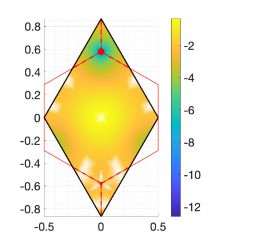
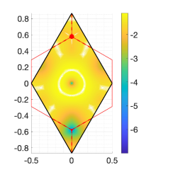
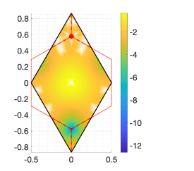
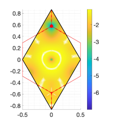
Figure 6. Modulus of flat band wavefunctions of $\ker_{X}(D(\alpha))$ at first magic angle $\alpha=0.853799$ with $X=L^{2}_{i,j}$ with $i=K$(top), $i=-K$ (bottom), $j=0$ (left), $j=1$ (right) for potential $U_{2}$ in (1.8).

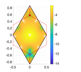
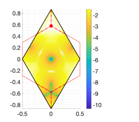
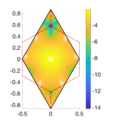
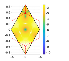
Figure 7. Flat band wavefunctions of $\ker_{X}(D(\alpha))$ at first magic angle $\alpha=0.853799$ with $X=L^{2}_{0,0}$ (left) and $X=L^{2}_{0,1}$ (right) for potential $U_{2}$ in (1.8) upper component, top and lower component, bottom.

We start with a simple Lemma

Lemma 7.1.

Let $u\in\ker_{L^{2}_{0,0}({\mathbb{C}}/\Lambda;{\mathbb{C}}^{2})}(D(\alpha))$ and $z_{S}:=i/\sqrt{3}$ then

$$u(z)=(z-z_{S})w_{1}(z)\text{ and }u(z)=(z+z_{S})w_{2}(z)\text{ with }w_{1},w_{2}\in C^{\infty}({\mathbb{C}};{\mathbb{C}}^{2}).$$

Let $u\in\ker_{L^{2}_{0,1}({\mathbb{C}}/\Lambda;{\mathbb{C}}^{2})}(D(\alpha))$ then

$$u(z)=z^{2}w(z),\text{ with }w\in C^{\infty}({\mathbb{C}};{\mathbb{C}}^{2}).$$

Proof.

Let $u\in\ker_{L^{2}_{0,0}({\mathbb{C}}/\Lambda;{\mathbb{C}}^{2})}(D(\alpha))$, $z_{S}=i/\sqrt{3}$ and $\omega z_{S}=z_{S}-(1+\omega).$ Thus

$$\begin{split}u(\pm z_{S})&=u(\pm\omega z_{S})=u(\pm z_{S}\mp(1+\omega))=\operatorname{diag}(e^{-i\langle\mp(1+\omega),K\rangle},e^{i\langle\mp(1+\omega),K\rangle})\mathscr{L}_{\mp(1+\omega)}u(\pm z_{S})\\ &=\operatorname{diag}(\omega^{\pm 1},\omega^{\mp 1})u(\pm z_{S}).\end{split}$$

This implies that $u(\pm z_{S})=0$. Due to [BHZ22b, Lemma $3.2$], we conclude that

$$u(z)=(z-z_{S})w_{1}(z)\text{ and }u(z)=(z+z_{S})w_{2}(z)$$

with $w_{1},w_{2}\in C^{\infty}({\mathbb{C}};{\mathbb{C}}^{2}).$

Let $u\in\ker_{L^{2}_{0,1}({\mathbb{C}}/\Lambda;{\mathbb{C}}^{2})}(D(\alpha))$, then since $u(\omega z)=\bar{\omega}u(z)$ we conclude that $u(0)=0.$ Again by [BHZ22b, Lemma $3.2$], we have $u(z)=z\tilde{w}(z)$ with $w\in C^{\omega}({\mathbb{C}};{\mathbb{C}}^{2}).$ Using that

$$\bar{\omega}u(z)=u(\omega z)=\omega z\tilde{w}(\omega z)$$

we conclude that $\omega z\tilde{w}(z)=\omega u(z)=z\tilde{w}(\omega z)$ which implies that $\omega\tilde{w}(z)=\tilde{w}(\omega z).$ If the zero of $\tilde{w}$ is of order one, then this implies that

$$u(z)=z^{2}w(z),\text{ with }w\in C^{\omega}({\mathbb{C}};{\mathbb{C}}^{2}).$$

∎

Theorem 8.

Let $\operatorname{dim}\ker_{L^{2}_{0,j}}(D(\alpha))\leq 1$ for all $j\in{\mathbb{Z}}_{3}$, then the zeros exhibited in Lemma 7.1 are the only ones counting multiplicity.

Proof.

We first show that the zeros occur only at the points specified in Lemma 7.1, i.e. $\{0,\pm z_{S}\}$. Suppose otherwise and that in addition $z_{0}\notin\{0,\pm z_{S}\}$. This way, $\omega^{j}z_{0}$ describe three distinct points ${\mathbb{C}}/\Gamma_{3}$. Thus, there exists a meromorphic function $g_{z_{0}}$ with poles of order one at points $\omega^{j}z_{0}+\Lambda$ and satisfying both translational and rotational symmetry

$$g_{z_{0}}(z+\gamma)=g_{z_{0}}(z),\ \ \gamma\in\Lambda,\ \ g_{z_{0}}(\omega z)=g_{z_{0}}(z).$$

One can then choose (see [Mu83, §I.6])

$$g_{z_{0}}(z)=c\prod_{j=0}^{2}\frac{\theta(z\omega^{j-1}+z_{0})}{\theta(z\omega^{j-1}-z_{0})}.$$

This way, the newly defined function $\widetilde{u}(z):=g_{z_{0}}(z)u(z)$ satisfies $D(\alpha)\widetilde{u}=0$ with $\widetilde{u}\in L^{2}_{{0,j}}({\mathbb{C}}/\Lambda)$ for $u\in L^{2}_{0,j}({\mathbb{C}}/\Lambda).$ Uniqueness of $u$ in representations $L^{2}_{0,j}$ implies that there is no such zero.

We now exclude further zeros at $0$. We recall that if $u\in\ker_{L^{2}_{0,j}({\mathbb{C}}/\Lambda;{\mathbb{C}}^{2})}(D(\alpha))$ with $j\in\{0,1\}$ has further zeros at $0$, then they have to be at least of the form $u(z)=z^{3}w(z)$ for $w$ smooth by rotational symmetry and by successively applying [BHZ22b, Lemma $3.2$]. From this it follows that

$$\widetilde{u}(z):=\wp^{\prime}(z;\omega,1)u\in L^{2}_{0,0}({\mathbb{C}}/\Lambda),$$ (7.5)

with $D(\alpha)\widetilde{u}=0$. Since the elements of the nullspace of $D(\alpha)$, $u$, are assumed to be unique up to a multiplicative constant, we conclude that this is impossible. (Here $\wp(z;\omega_{1},\omega_{2})$ is the Weierstrass $\wp$-function – see [Mu83, §I.6]. It is periodic with respect to ${\mathbb{Z}}\omega_{1}+{\mathbb{Z}}\omega_{2}$ and its derivative has a pole of order $3$ at $z=0$.)

Finally, we may now turn to $\pm z_{S}$. We start by showing that $u\in\ker_{L^{2}_{0,j}({\mathbb{C}}/\Lambda;{\mathbb{C}}^{2})}(D(\alpha))$ does not have a zero of second order at $\pm z_{S}.$ Indeed, if we assume that $z_{0}=\pm z_{S}$ is a zero of order 2, then since $\mathscr{E}$ leaves $L^{2}_{0,0}$ invariant, the zero at $z_{0}=\mp z_{S}$ is of second order as well. This is impossible as this implies the existence of four zeros which by the usual theta function argument, cf. [BHZ22b, Lemma $4.1$], allows us to construct four linearly independent elements of the nullspace of $D(\alpha).$ The same argument, using the symmetry $\mathscr{E}$, shows that $u\in\ker_{L^{2}_{0,1}({\mathbb{C}}/\Lambda)}(D(\alpha))$ cannot vanish at $\pm z_{S}.$ ∎

We record the following immediate consequence which will be useful later:

Lemma 7.2.

If $\operatorname{dim}\ker_{L^{2}_{0,j}}(D(\alpha))\leq 1$, for then $j\in\mathbb{Z}_{3}$,

$$\wp(z;\omega_{1},\omega_{2})\ker_{L^{2}_{0,1}({\mathbb{C}}/\Lambda;{\mathbb{C}}^{2})}(D(\alpha))=\ker_{L^{2}_{0,0}({\mathbb{C}}/\Lambda;{\mathbb{C}}^{2})}(D(\alpha)).$$

7.3. Generic magic angles

We already showed in Proposition 2.2 that $\operatorname{Spec}_{L^{2}_{0,0}}(RW)=\operatorname{Spec}_{L^{2}_{0,1}}(RW)$ and know from the previous Lemma that we can ensure simplicity of spectra of $RW$ in each representation $L^{2}_{0,j}$. We shall now see that we can split spectra of $RW$ in $L^{2}_{0,0},L^{2}_{0,1}$ from the one in $L^{2}_{0,2}.$

Lemma 7.3.

Suppose that

$$\operatorname{Spec}_{L^{2}_{{0,j}}}(RW)\cap D(\lambda_{0},2r)=\{\lambda_{0}\},\ \ \ j\in{\mathbb{Z}}_{3},\ r>0,$$

and $\lambda_{0}$ is a simple eigenvalue of $RW|_{L^{2}_{{0,j}}}$. Then, for every $\varepsilon>0$ there exists $V\in\mathscr{V}$, $\|V\|_{\delta}<\varepsilon$, such that for some $\lambda_{1}\neq\lambda_{2}$

$$\begin{split}&\operatorname{Spec}_{L^{2}_{{0,2}}}(R(W+V))\cap D(\lambda_{0},r)=\{\lambda_{2}\},\\ &\operatorname{Spec}_{L^{2}_{{0,j}}}(R(W+V))\cap D(\lambda_{0},r)=\{\lambda_{1}\},j\in\{0,1\}.\ \ \end{split}$$ (7.6)

Proof.

As in (6.15) we have ${w}_{k},\widetilde{w}_{k}\in L^{2}_{{0,j_{k}}}$, such that $\langle w_{k},\widetilde{w}_{k}\rangle=1$, and

$$(2\lambda_{0}D_{\bar{z}}-W){w}_{k}=0,\ \ \ (2\bar{\lambda}_{0}D_{z}-W^{*})R^{*}\widetilde{w}_{k}=0.$$

Since the eigenvalue $\lambda_{0}$ is assumed to be simple, (6.4) gives

$$R^{*}\widetilde{w}_{p}=\gamma_{1-p}\mathscr{A}w_{1-p}=\gamma_{1-p}\begin{pmatrix}\ \bar{w}_{(1-p)2}\\ -\bar{w}_{(1-p)1}\end{pmatrix},\ \ w_{p}=\begin{pmatrix}w_{p1}\\ w_{p2}\end{pmatrix},\ \ \gamma_{p}\in\mathbb{C}^{*}.$$ (7.7)

We can split an eigenvalue with eigenvectors $w_{k}$, if we can find $V$ such that (see (6.14) for the notation)

$$\begin{gathered}\langle Vw_{2},R^{*}\widetilde{w}_{2}\rangle_{L^{2}(F)}\neq\langle Vw_{0},R^{*}\widetilde{w}_{0}\rangle_{L^{2}(F)},\text{ with }\\ \langle Vw_{2},R^{*}\widetilde{w}_{2}\rangle=\bar{\gamma_{2}}\int_{F}\left(U_{+}(z)w_{22}^{2}(z)-U_{-}(z)w_{21}^{2}(z)\right)dm(z)\text{ and }\\ \langle Vw_{0},R^{*}\widetilde{w}_{0}\rangle=\bar{\gamma}_{1}\langle Vw_{0},\mathscr{A}w_{1}\rangle=\bar{\gamma_{1}}\int_{F}\left(U_{+}(z)w_{02}(z)w_{12}(z)-U_{-}(z)w_{01}(z)w_{11}(z)\right)dm(z)\end{gathered}$$

where we used (7.7) to obtain the last equality. If for all (analytic) $U_{\pm}$ the terms were equal it would follow that $\bar{\gamma_{2}}w_{2\ell}^{2}=\bar{\gamma_{1}}w_{0\ell}w_{1\ell}$ for $\ell\in\{1,2\}$. This implies that $w_{2\ell}$ vanishes at $0,\pm z_{S}$. However, the zeros at $\pm z_{S}$ have to be at least of order $2$ since by rotational and translational symmetry

$$\begin{split}w_{2}(z\pm z_{S})&=\bar{\omega}w_{2}(\omega(z\pm z_{S}))=\bar{\omega}w_{2}(\omega z\pm z_{S}\mp(1+\omega))\\ &=\bar{\omega}\operatorname{diag}(\omega^{\pm 1},\omega^{\mp 1})w(\omega z\pm z_{S}).\end{split}$$ (7.8)

This means that for instance at $z_{S}$ we have $w_{2}(z\pm z_{S})=\operatorname{diag}(1,\omega)w(\omega z\pm z_{S})$ which means that the first component has to vanish at least to third order and the second component at least to second order. This implies that $w_{2}$ has at least $5$ zeros counting multiplicities and this is impossible by the usual theta function argument [BHZ22b, Lemma $4.1$]. ∎

We can now finish

Proof of Theorem 3.

Lemma 6.2 (strictly speaking its proof) and Lemma 7.3 now show that for every $r>0$, the set

$$\mathscr{V}_{r}:=\{V:\text{ $RV|_{L^{2}_{0,1}\oplus L^{2}_{0,2}}$ has simple eigenvalues in $\mathbb{C}\setminus D(0,r)$}\}$$

is open and dense. We then obtain $\mathscr{V}_{0}$ by taking the intersection of $\mathscr{V}_{1/n}$. ∎

8. Spectral gap and Rigidity

In this section we prove Theorems 1 and 4, the two-fold degenerate magic angle rigidity and spectral gap between the flat bands and the rest of the spectrum.

Proof of Theorem 1.

From [BHZ22b, Theorem $2$] we know that if $\dim\ker_{L^{2}_{0}}(D(\alpha)+p)=2$ then $\dim\ker_{L^{2}_{0}}D(\alpha)\geq 2$. To obtain a contradiction, we suppose $\ker_{L^{2}_{0,1}}D(\alpha)=\{0\}$.

From Lemma 7.2 we conclude that $V:=\ker_{L^{2}_{0,2}}D(\alpha)\geq 2$. In fact, $\dim V=2$ or else the theta function argument, see [BHZ22b, Lemma 4.1], gives $\dim\ker_{L^{2}_{0}}(D(\alpha)+p)>2$. We decompose $V$ into the eigenspaces of $\mathscr{E}$. In particular we have a basis

$$u_{j}(z)=\begin{pmatrix}f_{j}(z)\\ \varepsilon_{j}if_{j}(-z)\end{pmatrix},\ \ \varepsilon_{j}\in\{\pm 1\},j\in\{1,2\}.$$

We conclude that $u_{j}$ can only vanish at $0$: otherwise there would be three zeros: $u_{j}(z_{0})=0$ then $u_{j}(-z_{0})=0$. And that is again impossible, see [BHZ22b, Lemma $4.1$]. So, we are in the situation of having two independent elements of $\ker_{L^{2}_{0,2}}D(\alpha)$ each with a simple zero at $0$. We want to show that

$$\ker_{L^{2}_{0}}(D(\alpha)+k)=Y_{k}:=\{G_{k,\lambda}(z):=F_{k}(z)(\lambda_{1}u_{1}(z)+\lambda_{2}u_{2}(z)):\lambda\in\mathbb{C}^{2}\}.$$

We claim that $G_{k,\lambda}(z)$ vanishes only at $z(k)+\Lambda^{*}$ where $z(k):={\sqrt{3}k}/{4\pi i}$. Otherwise for some $\lambda\in\mathbb{C}^{2}\setminus\{0\}$ and $z_{1}\notin\Lambda^{*}$, $\lambda_{1}u_{1}(z_{1})+\lambda_{2}u_{2}(z_{1})=0$, and that would mean that $W(u_{1},u_{2})\equiv 0$ and consequently $u_{1}(z)=g(z)u_{2}(z)$, where $g$ is a meromorphic function. But this leads to a contradiction as follows: $u_{j}(z)$ vanish simply at $z=0$ so $g(0)\neq 0$ and it has to vanish at at least two points (or have a double zero) - but that contradicts the uniqueness of the zero of $u_{j}$.

Now, suppose that $v_{k}\in\ker_{L^{2}_{0}}(D(\alpha)+k)$ we again conclude by the Wronskian argument (using the fact that $G_{k,\lambda}(z(k))=0$)

$$v_{k}(z)=g_{\lambda}(z)G_{k,\lambda}(z),$$

and $g_{\lambda}$ is nontrivial if we assume that $v_{k}$ is not in $Y_{k}$. But as $v_{k}$ was arbitrary that means that $u_{1}$ and $u_{2}$ have to be dependent. Hence, $\dim V=1$ which is the desired contradiction ∎

Proof of Theorem 4.

We need to show that there exists $p$ such that $\operatorname{dim}\ker_{L^{2}_{0}}(D(\alpha)+p)=2$ then this implies that for all $k\in\mathbb{C}$ we have $\operatorname{dim}\ker_{L^{2}_{0}}(D(\alpha)+k)=2$. As in the proof of Theorem 1, [BHZ22b, Theorem $2$] shows that $\dim\ker_{L^{2}_{0}}D(\alpha)\geq 2$ and consequently Theorem 1 shows that there exists $u\in\ker_{L^{2}_{0,1}}(D(\alpha))$. The rotational symmetry forces $u$ to vanish a second order at $0$, see Lemma 7.1. Hence, we can construct at least two linearly independent solution in $\ker_{L^{2}_{0}}(D(\alpha)+k)$ of the form

$$G_{k,r}(z):=F_{k+r}(z)F_{-r}(z)u(z)=\theta(z-z(k+r))\theta(z+z(r))e^{\frac{i}{2}k(z-\bar{z})}\frac{u(z)}{\theta(z)^{2}},$$ (8.1)

by taking two suitable choices of $r$. This is possible since the function $G_{k,r}$ has zeros at $z(k+r)$ and $z(-r)$ with $z(r):={\sqrt{3}r}/{4\pi i}$. We note that $\theta(z-z(k+r))\theta(z+z(r))\in\mathscr{G}_{k}$, where

$$\begin{gathered}\mathscr{G}_{k}=\{G\in\mathscr{O}(\mathbb{C}):G(z+\gamma)=e_{\gamma}(z)G(z),\ \gamma\in\Lambda\},\\ e_{1}=1,\ \ e_{\omega}(z)=e^{i\beta-4\pi iz},\ \ \beta=-2\pi i\omega^{2}+4\pi iz(k),\end{gathered}$$ (8.2)

and $e_{\gamma}$ is a multiplier in the sense of [BHZ22b, (B.2)]. We have, $\dim\mathscr{G}_{k}=2$ and $\mathscr{G}_{k}={\rm{span}}\{\theta(z-z(k+r))\theta(z+z(r)),r\in\mathbb{C}\}$ – see [TaZw23, Proposition 7.9] for an elementary argument or use the Riemann–Roch theorem.

Thus, it suffices to show that $\operatorname{dim}\ker_{L^{2}_{0}}(D(\alpha)+k)=2.$ We shall do this by showing that the space, defined using (8.1) or equivalently (8.2),

$$\begin{split}X_{k}&:=\operatorname{span}\{G_{k,r}:r\in{\mathbb{C}}\}=\mathscr{G}_{k}\cdot w\\ &\subset\ker_{L^{2}_{0}}(D(\alpha)+k),\ \ \ \ w(z):=e^{\frac{i}{2}(z-\bar{z})}u(z)/\theta(z)^{2}\end{split}$$ (8.3)

coincides with $\ker_{L^{2}_{0}}(D(\alpha)+k).$ Since its dimension is 2 that will prove the claim.

Let $v_{k}\in L^{2}_{0}$ be such that $(D(\alpha)+k)v=0.$ Our goal is to show that $v_{k}$ and $G_{k,r}$ are linearly dependent for some suitable $r$. Writing $v_{k}=(\varphi_{1},\varphi_{2})$ and $G_{k,r}=(\psi_{1},\psi_{2})$, then the Wronskian $W:=\varphi_{1}\psi_{2}-\varphi_{2}\psi_{1}$ satisfies

$$(2D_{\bar{z}}+k)W\equiv 0,\quad W(z+\gamma)=W(z),\quad\gamma\in\Lambda,$$

see [BHZ22b, (4.2)]. From $\mathscr{L}_{\gamma}u=u$, we find that $\varphi_{1}(z+\gamma)=e^{-i\langle\gamma,K\rangle}\varphi_{1}(z)$ and $\varphi_{2}(z+\gamma)=e^{i\langle\gamma,K\rangle}\varphi_{2}(z)$. Similar reasoning for $\psi_{1}$ and $\psi_{2}$ shows periodicity of $W$. Since $G_{k,r}$ has roots, it follows that $W$ vanishes at some $z_{0}$ and therefore $W\equiv 0.$ Indeed, if $k\notin\Lambda^{*}$, $W\equiv 0$ since $2D_{\bar{z}}+k$ is invertible. For $k\in\Lambda^{*}$ we have $W(z)=e^{-i\langle k,z-z_{1}\rangle}W(z_{0})=0$. This implies that

$$v_{k}(z)=g_{r}(z)G_{k,r}(z),\quad g_{r}(z+\gamma)=g_{r}(z),\quad z\in\Lambda$$ (8.4)

where $g_{r}(z)={\varphi_{1}}/{\psi_{1}}={\varphi_{2}}/{\psi_{2}}$ is a non-trivial meromorphic function if we assume that $v_{k}$ and $G_{k,r}$ are linearly independent. To see that the function is meromorphic, we notice that

$$2D_{\bar{z}}g_{r}(z)=\frac{(\psi_{1}2D_{\bar{z}}\varphi_{1}-\varphi_{1}2D_{\bar{z}}\psi_{1})(z)}{\psi_{1}(z)^{2}}=-k\frac{(\psi_{1}\varphi_{1}-\varphi_{1}\psi_{1})(z)}{\psi_{1}(z)^{2}}+\frac{U(z)W(z)}{\psi_{1}(z)^{2}}=0$$

showing holomorphy away from $\psi_{1}^{-1}(0)\cap\psi_{2}^{-1}(0)$. To see the meromorphic behaviour of $g_{r}$ at the set, see the argument in the paragraph after [BHZ22b, (4.4)]. In particular $g_{r}$ has at most $2$ poles.

If this was not the case then $G_{k,r}$ has at least three zeros. Let $w_{1}$ be one of the zeros, then $z\mapsto F_{-k}(z-w_{1})G_{k,r}(z)$ has also three zeros for $p$ as in our assumption. But then [BHZ22b, Lemma 4.1] provides a contradiction.

We also recall that, as a consequence of periodicity and the argument principle, the number of zeros of $g_{r}$ per fundamental cell coincides with the number of poles there. But then (8.4) shows that $v_{k}$ has to vanish at two points, say, $z_{1},z_{2}$. Put

$$v_{p}:=F_{p-k}(z-z_{1})v_{k}\in\ker_{L^{2}_{0}}(D(\alpha)+p).$$ (8.5)

In the notation of (8.3), $X_{p}\subset\ker_{L^{2}_{0}}(D(\alpha)+p)$ and as both vector spaces have the same dimension, they are equal. Thus, it follows that $v_{p}\in X_{p}:=\operatorname{span}\{G_{p,r},r\in{\mathbb{C}}\}$ with zeros $z_{2},z_{3},$ where $z_{3}$ satisfies $F_{p-k}(z_{3}-z_{1})=0.$

Then, we can choose $r$ such that $z(-r)=z_{3}$ and define $z_{4}:=z(p+r)$ such that both $z(-r^{\prime}),z(p+r^{\prime})\notin\{z_{3},z_{4}\}$. This ensures that $G_{p,r}$ and $G_{p,r^{\prime}}$ are linearly independent elements in $X_{p}$ and form a basis. We conclude that $v_{p}=\lambda_{1}G_{p,r}+\lambda_{2}G_{p,r^{\prime}}$, for some $\lambda_{1},\lambda_{2}$. Since $v_{p}(z_{3})=G_{p,r}(z_{3})=0$ and $G_{p,r^{\prime}}(z_{3})\neq 0$, this implies that $\lambda_{2}=0$ and thus $v_{p}=\lambda_{1}G_{p,r}.$ By inverting (8.5), we find

$$v_{k}=\frac{v_{p}}{F_{p-k}(\bullet-z_{1})}=\lambda_{1}\frac{G_{p,r}}{F_{p-k}(\bullet-z_{1})}=\tilde{\lambda}_{1}G_{k,s},$$

where $\tilde{\lambda}_{1}=e^{-i(p-k)(z_{1}-\bar{z}_{1})}\lambda_{1}$ and $s=p+r$. Hence an arbitrary $v_{k}\in\ker_{L^{2}_{0,1}}(D(\alpha)+k)$ is in $X_{k}$, that is $X_{k}=\ker_{L^{2}_{0,1}}(D(\alpha)+k)$ as claimed. ∎

9. The Chern number of a 2-degenerate flat band

In this section we compute the Chern number of the flat band in the case of 2-fold degeneracy. We start by a general discussion of of the Chern connection and the Berry connection in the case holomorphic vector bundles. Although we stress our case of the two torus, §§9.1 and 9.2 apply to vector bundles over more general manifolds.

9.1. The Chern connection

Suppose that $\pi:E\mapsto X$ is a holomorphic vector bundle over a torus $X=\mathbb{C}/\Lambda^{*}$ (see [TaZw23, §2.7] for a quick introduction sufficient for our purposes or [We07] for an in-depth treatment), and that $E$ is a sub-bundle of a trivial Hilbert bundle over $X$, $X\times\mathscr{H}$, where $\mathscr{H}$ is a Hilbert space. This gives a hermitian structure on $E$: for $k\in X$, we introduce an inner product on the fibers $E_{k}:=\pi^{-1}(k)$, using $E_{k}\subset\mathscr{H}$:

$$\langle\zeta,\zeta^{\prime}\rangle_{k}:=\langle\zeta,\zeta^{\prime}\rangle_{\mathscr{H}},\ \ \ \zeta,\zeta^{\prime}\in E_{k}.$$

We then have two natural connections on $E$, the Chern connection, available when the bundle is holomorphic and equipped with hermitian structure, and a hermitian connection, available for any smooth vector bundle embedded in a Hilbert bundle. In the context of vector bundles of eigenfunctions, the latter is called the Berry connection and we adopt this terminology for the general case as well.

We first define the Chern connection. For that we choose a local holomorphic trivialization $U\subset X$, $\pi^{-1}(U)\simeq U\times\mathbb{C}^{n}$, for which the hermitian metric is given by

$$\langle\zeta,\zeta\rangle_{k}=\langle G(k)\zeta,\zeta\rangle=\sum_{i,j=1}^{n}G_{ij}(k)\zeta_{i}\bar{\zeta}_{j}\ \ \zeta\in\mathbb{C}^{n},\ \ k\in U.$$ (9.1)

We note that if $\{u_{1}(k),\ldots,u_{n}(k)\}\subset\mathscr{H}$ is a basis of $E_{k}$ for $k\in U$, and $U\ni k\to u_{j}(k)$ are holomorphic, then $G(k)$ is the Gramian matrix:

$$G(k):=\left(\langle u_{i}(k),u_{j}(k)\rangle_{\mathscr{H}}\right)_{1\leq i,j\leq n}.$$ (9.2)

If $s:X\to E$ is a section, then the Chern connection $D_{C}:C^{\infty}(X;E)\to C^{\infty}(X;E\otimes T^{*}X)$, over $U$ is given by (using only the local trivialization and (9.1))

$$\begin{gathered}D_{C}s(k):=ds(k)+\eta_{C}(k)s(k),\\ \eta_{C}(k):=G(k)^{-1}\partial_{k}G(k)\,dk\in C^{\infty}(U,\operatorname{Hom}(\mathbb{C}^{n},\mathbb{C}^{n})\otimes(T^{*}U)^{1,0}).\end{gathered}$$ (9.3)

Here $\partial_{k}$ denotes the holomorphic derivative and the notation $(T^{*}U)^{1,0}$ indicates that only $dk$ and not $d\bar{k}$ appear in the matrix valued 1-form $\eta_{C}$, $\eta_{C}=\eta_{C}^{1,0}$. We also recall that $D_{C}$ is the unique hermitian connection with this property – see [We07, Theorem 2.1].

For the definition of the Berry connection we only require that $E\to X$ is a smooth vector bundle which is a subbundle of $X\times\mathscr{H}$, where $\mathscr{H}$ is a Hilbert space. That means for $k\in X$ we have a well defined orthogonal projection $\Pi(k):\mathscr{H}\to E_{k}:=\pi^{-1}(k)$ and an inclusion map $\iota:E\hookrightarrow X\times\mathscr{H}$. The formula for the Berry connection is then given by

$$D_{B}s(k):=\Pi(k)(d(\iota\circ s)(k)).$$ (9.4)

To find a local expression similar to (9.3) we use the Gramian (9.2). If $s(k)=\sum_{j=1}^{n}s_{j}^{U}(k)u_{j}(k)=:A(k)s^{U}(k)$, $A(k):\mathbb{C}^{n}\to\mathscr{H}$ (so that $A(k)$ provides a local trivialization) then $\Pi(k)=A(k)G(k)^{-1}A(k)^{*}$ and

$$\begin{gathered}\begin{split}D_{B}s(k)&=\Pi(k)\sum_{j=1}^{n}\left(ds_{j}^{U}(k)u_{j}(k)+s_{j}^{U}(k)du_{j}(k)\right)\\ &=A(k)(ds^{U}(k)+\eta_{B}(k)s^{U}(k)),\end{split}\\ \eta_{B}(k)=G(k)^{-1}B(k)\in C^{\infty}(U,\operatorname{Hom}(\mathbb{C}^{n},\mathbb{C}^{n})\otimes T^{*}U),\\ B(k)_{\ell j}:=\langle du_{j}(k),u_{\ell}(k)\rangle_{\mathscr{H}}\in C^{\infty}(U,T^{*}U).\end{gathered}$$ (9.5)

These formulas hold for choices of $u_{j}$ which are not necessarily holomorphic. However if, as in (9.2), $k\mapsto u_{j}(k)$ are holomorphic, then

$$\begin{split}(\partial_{k}G(k))_{ij}dk&=\langle\partial_{k}u_{i}(k),u_{j}(k)\rangle_{\mathscr{H}}dk+\langle u_{i}(k),\partial_{\bar{k}}u_{j}(k)\rangle_{\mathscr{H}}dk\\ &=\langle\partial_{k}u_{i}(k),u_{j}(k)\rangle_{\mathscr{H}}dk\\ &=\langle du_{i}(k),u_{j}(k)\rangle=B(k)_{ij},\end{split}$$ (9.6)

since $\partial_{\bar{k}}u_{j}(k)=0$ and $dw=\partial_{k}w\,dk+\partial_{\bar{k}}w\,d\bar{k}$. In particular, that means that in the notation of (9.3) and (9.4)

$$\begin{split}\text{$U\ni k\mapsto u_{\ell}(k)$ holomorphic }&\ \Longrightarrow\ \ \eta_{C}(k)=\eta_{B}(k),\ k\in U\\ &\ \Longrightarrow\ \ D_{C}=D_{B},\end{split}$$ (9.7)

We record this standard fact as

Proposition 9.1.

Suppose that $X$ is a complex manifold and $E\mapsto X$ is a holomorphic vector bundle with a holomorphic embedding $\iota:E\to X\times\mathscr{H}$ into a trivial Hilbert bundle. Then the Berry connection (9.4) and the Chern connection (9.3) defined using the hermitian structure on $\mathscr{H}$ are equal.

Remark. As was pointed out to us by Michael Singer, the conclusion (9.7) could be deduced directly from the uniqueness of the Chern connection mentioned after (9.3): using (9.4) we have $D_{B}^{(0,1)}s(k)=\Pi(k)(d^{(0,1)}(\iota\circ s)(k))$. But as the embedding $\iota$ (an inclusion, in our case) is holomorphic this implies that $D_{B}^{(0,1)}s(k)=0$ for holomorphic sections. This and being hermitian characterize the Chern connection. We should also stress that the discussion above does not depend on the fact that $X$ has complex dimension one.

The curvature of a connection $D$ is given by

$$\Theta:=D\circ D,$$ (9.8)

which is a globally defined two form with values in $\operatorname{Hom}(E,E)$. In a local trivialization in which $D=d+\eta$, we have $\Theta=d\eta+\eta\wedge\eta$. For the Chern connection, for $X$ of any dimension $\Theta=\bar{\partial}\partial\eta_{C}$ since (9.3) shows that $\partial\eta_{C}=-\eta_{C}\wedge\eta_{C}$ (when $X$ has a complex dimension one, this is obvious as $dk\wedge dk=0$). It is then immediate from (9.7) that

$$\Theta:=D_{C}\circ D_{C}=D_{B}\circ D_{B},$$ (9.9)

that is, in the holomorphic case, the curvatures defined using the Chern curvature or the Berry curvature agree for holomorphic vector bundles embedded in trivial Hilbert bundles.

The Chern class (a Chern number in the case of $\mathbb{C}/\Lambda^{*}$) is given by

$$c_{1}(E):=\frac{i}{2\pi}\int_{\mathbb{C}/\Lambda^{*}}\operatorname{tr}\Theta\in\mathbb{Z},$$

where we note that over $U\subset\mathbb{C}/\Lambda^{*}$ for which we defined (9.2),

$$\begin{split}\operatorname{tr}\Theta&=\partial_{\bar{k}}\operatorname{tr}G(k)^{-1}\partial_{k}G(k)\,d\bar{k}\wedge dk\\ &=\partial_{\bar{k}}\partial_{k}\log g(k)\,d\bar{k}\wedge dk,\ \ \ \ g(k):=\det G(k),\end{split}$$ (9.10)

where we used Jacobi’s formula [DyZw19, (B.5.14)]. In particular,

$$H(k):=\partial_{\bar{k}}\partial_{k}\log g(k)=g(k)^{-2}(g(k)\partial_{\bar{k}}\partial_{k}g(k)-|\partial_{k}g(k)|^{2}).$$

For any holomorphic hermitian vector bundle the trace of the curvature of the Chern connection, $\operatorname{tr}\Theta$ can be interpreted as a curvature of a line bundle. If $\pi:E\to X$ has rank $n$, we obtain a line bundle $\pi:L:=\wedge^{n}E\to X$. It inherits hermitian structure from $E$. If we define the Chern connection on $\wedge^{n}E$ as in (9.3) (using only holomorphy and the hermitian structure) we obtain a new curvature $\Theta_{L}$ which is a differential two form on $X$, and

$$\Theta_{L}=\operatorname{tr}\Theta.$$

In case when $E$ embeds holomorphically in $X\times\mathscr{H}$ we can then take, as in (9.2), $k\mapsto u_{j}(k)\in\mathscr{H}$, $j=1,\cdots,n$, a local holomorphic basis of $E$. Then for

$$\Phi(k):=\wedge_{j=1}^{n}u_{j}(k)\in\wedge^{n}E_{k}\subset\wedge^{n}\mathscr{H},$$ (9.11)

we have

$$\|\Phi(k)\|^{2}_{\wedge^{n}\mathscr{H}}=\det\left((\langle u_{j}(k),u_{\ell}(k)\rangle_{\mathscr{H}})_{1\leq j,\ell\leq n}\right)=\det G(k)=g(k).$$

In particular when $X=\mathbb{C}/\Lambda^{*}$, we obtain, as in [BHZ22b, (5.10)], $\Theta_{L}=H(k)d\bar{k}\wedge dk$ with

$$H(k)=\|\Phi(k)\|^{-4}\left(\|\Phi(k)\|^{2}\|\partial_{k}\Phi(k)\|^{2}-|\langle\partial_{k}\Phi(k),\Phi(k)\rangle|^{2}\right)\geq 0,$$ (9.12)

where $\|\bullet\|=\|\bullet\|_{\wedge^{n}\mathscr{H}}$.

Remark. From a physics perspective the construction of the line bundle $\wedge^{n}E$, in the case of $E\subset X\times\mathscr{H}$ can be interpreted as the Slater determinant of the individual Bloch functions on the fermionic $n$-particle Hilbert space. We thus find that the trace of the curvature of the rank $n$ vector bundle coincides with the curvature of the line bundle described by the $n$-particle wavefunction.

9.2. The Berry curvature

For completeness we derive the standard formula for the curvature of the Berry connection (9.4):

Proposition 9.2.

Suppose that $\pi:E\to X$ is a complex vector bundle over a manifold $X$ and that there exists an embedding $\iota:E\to X\times\mathscr{H}$ into a trivial Hilbert bundle. Then the curvature of the connection (9.4) is given in terms of the orthogonal projection $\Pi(k):\mathscr{H}\to E_{k}:=\pi^{-1}(k)$, as

$$\Theta=\Pi\,d\Pi\wedge d\Pi|_{E},$$ (9.13)

and is a differential two form with values in $\operatorname{Hom}(E,E)$.

Proof.

This is a local computation so for some $U\subset X$ we can choose a smoothly varying orthonormal basis $\{u_{j}(k)\}_{j=1}^{n}$, $k\in U$. Then in the notation of (9.5) (we drop the dependence on $k$ in $A(k)$, $\Pi(k)$ and $E_{k}$)

$$A:\mathbb{C}^{n}\to\mathscr{H},\ \ A^{*}:\mathscr{H}\to\mathbb{C}^{n},\ \ \ AA^{*}=\Pi,\ \ A^{*}A=I_{\mathbb{C}^{n}}.$$ (9.14)

With the trivialization given by $A$, we have (using (9.14))

$$Ds=A^{*}(\Pi(d(As))=A^{*}\Pi Ads+A^{*}\Pi dAs=ds+A^{*}dAs=:ds+\eta ds.$$

Hence, in this trivialization, the curvature is a differential two form with values in $\operatorname{Hom}(\mathbb{C}^{n},\mathbb{C}^{n})$:

$$\begin{split}A^{*}\Theta A&=d\eta+\eta\wedge\eta=d(A^{*}dA)+A^{*}dA\wedge A^{*}dA\\ &=dA^{*}\wedge dA+A^{*}dA\wedge A^{*}dA.\end{split}$$

The curvature $\Theta=D_{B}\circ D_{B}$ which is a differential form with values in $\operatorname{Hom}(E,E)$, is then given by

$$\begin{split}\Theta&=\Pi\Theta\Pi=A(dA^{*}\wedge dA+A^{*}dA\wedge A^{*}dA)A^{*}\\ &=AdA^{*}\wedge dAA^{*}+AA^{*}dA\wedge A^{*}dAA^{*}\\ &=AdA^{*}\wedge dAA^{*}+AdA^{*}A\wedge dA^{*}AA^{*},\end{split}$$ (9.15)

where we used $d(A^{*}A)=0$.

The right hand side in (9.13) is given by

$$\begin{split}AA^{*}d(AA^{*})\wedge d(AA^{*})&=AA^{*}((dAA^{*}+AdA^{*})\wedge(dAA^{*}+AdA^{*})\\ &=AA^{*}\left(dA\wedge(A^{*}dA)A^{*}+dA\wedge(A^{*}A)dA^{*}\right.\\ &\ \ \ \ \ \left.+AdA^{*}\wedge dAA^{*}+AdA^{*}\wedge dAA^{*}\right).\end{split}$$

From (9.14) we see that $A^{*}A=I_{\mathbb{C}^{n}}$ and that $A^{*}dA=-dA^{*}A$. Hence,

$$\begin{split}\Pi d\Pi\wedge d\Pi&=AA^{*}\left(-dA\wedge dA^{*}AA^{*}+dA\wedge dA^{*}\right.\\ &\ \ \ \ \ +\left.AdA^{*}\wedge dAA^{*}+AdA^{*}\wedge AdA^{*}\right).\end{split}$$

Acting on $E$, $AA^{*}=I_{E}$ and hence the first two terms in the bracket cancel:

$$\Pi d\Pi\wedge d\Pi|_{E}=AdA^{*}\wedge dAA^{*}|_{E}+AdA^{*}\wedge AdA^{*}|_{E}.$$

But from (9.15) that is the same as the action of $\Theta$ on $E$.

∎

9.3. Flat bands of multiplicity $2$ and proof of Theorem 5

We now consider

$$V(k):=\ker_{H^{1}_{0}}(D(\alpha)+k)\subset L^{2}_{0}.$$ (9.16)

This defines a (trivial) vector bundle $\widetilde{E}\to\mathbb{C}$:

$$\widetilde{E}:=\{(k,v):v\in V(k)\}\subset\mathbb{C}\times L^{2}_{0}(\mathbb{C}/\Lambda;\mathbb{C}^{2}).$$

To define a vector bundle over the torus $\mathbb{C}/\Lambda^{*}$ we define an equivalence relation on $\mathbb{C}\times L^{2}_{0}(\mathbb{C}/\Lambda;\mathbb{C}^{2})$:

$$\begin{gathered}\exists\,p\in\Lambda^{*}\ (k,u)\sim_{\tau}(k+p,\tau(p)^{-1}u),\ \ [\tau(p)u](z)=e^{i\langle z,k\rangle}v(z),\end{gathered}$$ (9.17)

and notice that $\tau(p)^{-1}V(k)=V(k+p)$. Using this (see [TaZw23, Lemma 8.4] or [BHZ22b, Lemma 5.1]),

$$E:=\widetilde{E}\,/\sim_{\tau}\,\to\mathbb{C}/\Lambda^{*}.$$ (9.18)

is a holomorphic vector bundle over $\mathbb{C}/\Lambda^{*}$.

Since $\Pi(k+p)=\tau(p)^{-1}\Pi(k)\tau(p)$, the Berry connection defined by (9.4) on $\widetilde{E}$, satisfies

$$(D_{B}s)(k+p)=\Pi(k+p)(d(\iota\circ s)(k+p))=\tau^{-1}(p)\Pi(k)d(\iota\circ\tau(p)s(k+p)).$$

Hence, if for $k\in U\subset X$, $(k,s(k))\sim_{\tau}(k^{\prime},s^{\prime}(k^{\prime}))$ then $k^{\prime}=k+p$, $s^{\prime}(k+p)=\tau(p)^{-1}s(k)$, for some $p\in\Lambda^{*}$ and

$$(k,D_{B}s(k))\sim_{\tau}(k^{\prime},D_{B}s^{\prime}(k^{\prime})).$$

This means that $D_{B}$ is a well defined connection on $\widetilde{E}$. Since the Chern connection is intrinsically defined on $\widetilde{E}$ using holomorphic and hermitian structures, the two connections are equal.

We now assume that $\dim V(k)=2$. Theorem 8 then shows that there exists $u_{0}\in L^{2}_{0,0}$ with simple zeros at $\pm z_{S}+\Lambda^{*}$. This allows us a characterization of $V(k)$ when $k\notin\Lambda^{*}$:

$$V(k)=\{\zeta_{1}F_{k}(z+z_{S})u_{0}(z)+\zeta_{2}F_{k}(z-z_{S})u_{0}(z),\ \zeta=(\zeta_{1},\zeta_{2})\in\mathbb{C}^{2}\},\quad k\notin\Lambda^{*}.$$ (9.19)

Remark. The space $V(k)$ could have been constructed equally well using $u_{1}\in\ker_{L^{2}_{0,1}}D(\alpha)$ even though the spaces appear to be different. Instead of (9.19) we could have taken

$$W(k):=\{\zeta_{1}F_{k}(z+z_{S})u_{0}(z)+\zeta_{2}F_{k}(z)u_{1}(z),\zeta\in\mathbb{C}^{2}\},\quad k\notin-K+\Lambda^{*}.$$ (9.20)

We can take $u_{1}(z)=F_{K}(z)^{-1}F_{-K}(z)^{-1}u_{0}(z)$ (giving the condition on $k$ in (9.20)). That the spaces have to coincide follows from the properties (8.2) in the proof of Theorem 4. An explicit map between the spaces $V(k)$ and $W(k)$ can be constructed using a theta function identity [KhZa15, (3.4)].

Returning to (9.19) we recall [BHZ22b, Lemma 3.3] for $p\in\Lambda^{*}$,

$$\begin{gathered}F_{k+p}(z)=e_{p}(k)^{-1}\tau(p)F_{k}(z),\\ e_{p}(k):=\frac{\theta(z(k))}{\theta(z(k+p))}=(-1)^{n}(-1)^{m}e^{i\pi n^{2}\omega+2\pi inz(k)},\end{gathered}$$ (9.21)

where $z(p)=m+n\omega$, $n,m\in\mathbb{Z}$. We define the Gramian (9.2) using

$$u_{j}(k)(z):=u_{0}(z)F_{k}(z-(-1)^{j}z_{S}),\ \ j=1,2,\ \ k\notin\Lambda^{*},$$

so that, for $p\in\Lambda^{*}$,

$$\begin{split}G_{\ell m}(k+p)&=\langle F_{k+p}(\bullet-(-1)^{\ell}z_{S})u_{0},F_{k+p}(\bullet-(-1)^{m}(z-(-1)^{m}z_{S})u_{0}\rangle\\ &=\langle e_{p}(k)^{-1}e^{i\langle\bullet-(-1)^{\ell}z_{S},p\rangle}u_{\ell},e_{p}(k)^{-1}e^{i\langle\bullet-(-1)^{m}z_{S},p\rangle}u_{m}\rangle\\ &=e^{i((-1)^{m}-(-1)^{\ell})\langle z_{S},p\rangle}|e_{p}(k)|^{-2}G_{\ell m}(k).\end{split}$$

This shows that

$$|e_{p}(k)|^{4}g(k+p)=g(k),\ \ \ k\notin\Lambda^{*}.$$ (9.22)

We should stress that even though $\log g(k)$ is not well defined at $k\in\Lambda^{*}$,

$$H(k):=\partial_{\bar{k}}\partial_{k}\log g(k)\in C^{\infty}(\mathbb{C}\setminus\Lambda^{*}),\ \ \ H(k+p)=H(k),\ \ k\notin\Lambda^{*},\ p\in\Lambda^{*}$$ (9.23)

extends to a smooth function in $\mathbb{C}$. That follows from the fact that $\operatorname{tr}\Theta=d(g^{-1}dg)=Hd\bar{k}\wedge dk$ is a well defined 2-form on $\mathbb{C}/\Lambda^{*}$. We now choose an interior of a fundamental domain of $\Lambda^{*}$, $F:=\{t+s\omega:-2\pi/\sqrt{3}<t,s,<2\pi/\sqrt{3}\}$ so that

$$\begin{split}c_{1}(E)&=\frac{i}{2\pi}\int_{F}\operatorname{tr}\Theta=\frac{i}{2\pi}\lim_{\varepsilon\to 0}\int_{F\setminus D(0,\varepsilon)}\partial_{\bar{k}}\partial_{k}\log g(k)d\bar{k}\wedge dk\\ &=\frac{i}{2\pi}\int_{\partial F}\partial_{k}\log g(k)dk-\frac{i}{2\pi}\lim_{\varepsilon\to 0}\int_{\partial D(0,\varepsilon)}\partial_{k}\log g(k)dk.\end{split}$$ (9.24)

Using (9.22) we see that

$$\frac{i}{2\pi}\int_{\partial F}\partial_{k}\log g(k)dk=-2.$$

(See [BHZ22b, (5.9),(B.8)] for a similar calculation.)

It remains to evaluate the limit on the right hand side of (9.24). We note that $g(k)\geq 0$ and $g(k)=0$ for $k\in\Lambda^{*}$ only. We write $F_{j}=F_{j}(k,z)=F_{k}(z-(-1)^{j}z_{S})$, $F_{j}^{\prime}=\partial_{k}F_{j}$. We then use (9.11) with $n=2$, and $\Phi(k)=F_{1}(k)u_{0}\wedge F_{2}(k)u_{0}$, which gives (using $\|u_{0}\|=1$, $F_{j}(0,z)=1)$,

$$\begin{split}\partial_{\bar{k}}\partial_{k}g(k)|_{k=0}&=\langle\partial_{k}\Phi(k),\partial_{k}\Phi(k)\rangle_{\wedge^{2}L^{2}_{0}}|_{k=0}=\|F_{1}^{\prime}u_{0}\wedge u_{0}+u_{0}\wedge F_{2}^{\prime}u_{0}\|_{\wedge^{2}L^{2}_{0}}>0\end{split}$$ (9.25)

unless $F_{1}^{\prime}u_{0}\wedge u_{0}=F_{2}^{\prime}u_{0}\wedge u_{0}$. Since

$$\begin{split}F_{1}^{\prime}(0,z)-F_{2}^{\prime}(0,z)&=i(z_{S}-\bar{z}_{S})+\frac{\sqrt{3}}{4\pi i}\left(\frac{\theta^{\prime}(z-z_{S})}{\theta(z-z_{S})}-\frac{\theta^{\prime}(z+z_{S})}{\theta(z+z_{S})}\right)\\ &\sim\pm\frac{\sqrt{3}}{4\pi i(z\mp z_{S})},\ \ \ z\sim\pm z_{S},\end{split}$$

this is clear impossible. Since $\Phi(0)=g(0)=0$, $\partial_{k}^{2}g(k)|_{k=0}=\langle\partial_{k}^{2}\Phi(0),\Phi(0)\rangle=0$, and hence, $g(k)=g_{0}|k|^{2}+\mathcal{O}(|k|^{3})$, $g_{0}>0$. It is now easy to evaluate the limit on the right hand side of (9.24):

$$\begin{split}-\frac{i}{2\pi}\lim_{\varepsilon\to 0}\int_{\partial D(0,\varepsilon)}\partial_{k}\log g(k)dk&=-\frac{i}{2\pi}\lim_{\varepsilon\to 0}\int_{\partial D(0,\varepsilon)}\partial_{k}\log(g_{0}|k|^{2}+\mathcal{O}(|k|^{3})dk\\ &=-\frac{i}{2\pi}\lim_{\varepsilon\to 0}\int_{\partial D(0,\varepsilon)}\frac{g_{0}\bar{k}+\mathcal{O}(|k|^{2})}{g_{0}|k|^{2}+\mathcal{O}(|k|^{3})}dk\\ &=-\frac{i}{2\pi}\lim_{\varepsilon\to 0}\int_{\partial D(0,\varepsilon)}(k^{-1}+\mathcal{O}(1))dk\\ &=-\frac{i}{2\pi}\lim_{\varepsilon\to 0}(2\pi i+\mathcal{O}(\varepsilon))=1.\end{split}.$$

Returning to (9.24) we have proved that $c_{1}(E)=-1$.

Finally, we observe that for $\Omega:L^{2}_{0}(\mathbb{C}/\Lambda;\mathbb{C})\to L^{2}_{0}(\mathbb{C}/\Lambda;\mathbb{C})$, $\Omega u(z):=u(\omega z)$, $\ker_{H^{1}_{0}}(D(\alpha)+\bar{\omega}k)=\Omega\ker_{H^{1}_{0}}(D(\alpha)+k)$ (see [BHZ22b, §2.1]). Hence, in the notation of (9.4). $\Omega\Pi(k)\Omega^{*}=\Pi(\bar{\omega}k)$. Hence, if $Rk:=\bar{\omega}k$, this means that $R^{*}\Pi=\Omega\Pi\Omega^{*}$. Also the pull back of $\Theta$ by $R$ is well defined and, using (9.13) we see that

$$R^{*}\Theta=R^{*}(\Pi d\Pi\wedge d\Pi)=R^{*}\Pi d(R^{*}\Pi)\wedge d(R^{*})\Pi=\Omega(\Pi d\Pi\wedge d\Pi)\Omega^{*}=\Omega\Theta\Omega^{*}.$$

In particular, in the notation of (9.23), we have

$$\operatorname{tr}R^{*}\Theta=\operatorname{tr}\Theta\ \Longrightarrow\ H(\bar{\omega}k)=H(k).$$

Strictly speaking we should, just as we did at the end of (9.18), justify passing to the quotient. That is again easy by noting that $\Omega\tau(p)\Omega^{*}=\tau(\bar{\omega}p)$. This completes the proof of Theorem 5.

$X=L^{2}_{0,2}$	$X=L^{2}_{0,0}$	$X=L^{2}_{0,1}$
1.2400 – 0.0000i	1.6002 + 0.0000i	1.6002 + 0.0000i
1.2400 – 0.0000i	1.2583 – 1.1836i	1.2583 – 1.1836i
1.3424 + 1.6788i	1.2583 + 1.1836i	1.2583 + 1.1836i
1.3424 – 1.6788i	1.4019 – 2.2763i	1.4019 – 2.2763i
2.9543 + 0.0000i	1.4019 + 2.2763i	1.4019 + 2.2763i
1.4575 + 2.7610i	1.5001 + 3.3130i	1.5001 + 3.3130i
1.4575 – 2.7610i	1.5001 – 3.3130i	1.5001 – 3.3130i
3.5878 + 1.9298i	3.4078 + 1.3122i	3.4078 + 1.3122i
3.5878 – 1.9298i	3.4078 – 1.3122i	3.4078 – 1.3122i

Table 2. Magic angles for $\theta=2.808850897$ and $U_{0}(\zeta)=\cos(\theta)U_{1}(\zeta)+\sin(\theta)\sum_{i=0}^{2}\omega^{i}e^{-(\zeta\bar{\omega}^{i}-\bar{\zeta}\omega^{i})}$ such that $1/\alpha\in\operatorname{Spec}_{X}(T_{0})$ (counting algebraic multiplicity). The magic angle with algebraic multiplicity $2$ and geometric multiplicity $1$ is highlighted in blue.

10. Numerical observations

Here we present two numerical observations related to our mathematical results.

10.1. Algebraic multiplicities in the spectral characterization

Theorem 1 implies that it is impossible to have

$$\dim\ker_{L_{0}^{2}}(D(\alpha))=\dim\ker_{L_{0,2}^{2}}(D(\alpha))=2$$

which is equivalent to having eigenvalues of geometric multiplicity $2$ for $T_{0}$, i.e.

$$\dim\ker_{L^{2}_{0}}(T_{0}-1/\alpha)=\dim\ker_{L^{2}_{0,2}}(T_{0}-1/\alpha)=2,$$

we can indeed have that $1/\alpha$ is an eigenvalue of algebraic multiplicity $2$ and geometric multiplicity $1$ on $L^{2}_{0}$ and $L^{2}_{0,2}.$ This is illustrated in Table 2 and Figure 9. In particular, it implies that $T_{k}$ in general is not diagonalizable. Since the algebraic multiplicity of $T_{k}$ is independent of $k$, it follows by Theorem 4 and its analogue in [BHZ22b] for simple and two-fold degenerate magic angles, that the geometric multiplicity is independent of $k$. Examples of this are exhibited in Table 2 and Figures 9 and 10.

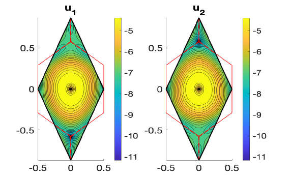
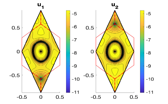
Figure 9. The first two singular values of $D(\alpha)$ are $2.804e-15$ and $3.990$ suggesting the existence of only one flat band at $\alpha=1.2400$ for $\theta=2.808850$ and $U_{0}(\zeta)=\cos(\theta)U_{1}(\zeta)+\sin(\theta)\sum_{i=0}^{2}\omega^{i}e^{-(\zeta\bar{\omega}^{i}-\bar{\zeta}\omega^{i})}$. The eigenvector of $T_{0}$ with eigenvalue $1/\alpha$ is shown on top and the generalized one at the bottom.

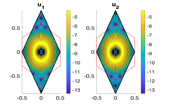
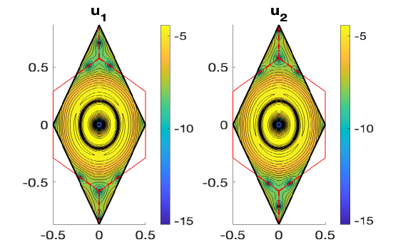
Figure 10. One flat band for $\alpha=5.3811$ for $\theta=2.7672151$ and $U_{0}(\zeta)=\cos(\theta)U_{1}(\zeta)+\sin(\theta)\sum_{i=0}^{2}\omega^{i}e^{-(\zeta\bar{\omega}^{i}-\bar{\zeta}\omega^{i})}$. The eigenvector of $T_{0}$ with eigenvalue $1/\alpha$ is shown on top and the generalized one at the bottom.

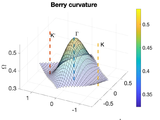
Figure 11. The plot of the curvature of the holomorphic line bundle corresponding to the first two-fold generate magic angle, defined in (9.23) with potential $U_{2}$, as in (1.8). The extrema at $K,\Gamma,K^{\prime}$ follow from Theorem 5.

Figure 12. Cross-section of curvature for $k_{x}=0$ for the first seven magic angles with potential $U_{2}$, as in (1.8), in increasing order. The extrema at $K,\Gamma,K^{\prime}$ follow from Theorem 5.

10.2. Behaviour of the curvature

Since we established in Theorem 5 that $H(\omega z)=H(z)$ where $H$ is the scalar curvature. We conclude that $0$ and $\pm z_{S}$ are critical points of $H$. In addition, the symmetry $\mathscr{E}$ defined in (2.12) and the formula (7.4) imply that the Gramian matrix satisfies for simple or two-fold degenerate magic angles

$$G(k)=G(-k).$$

This implies the symmetries in Figure 11.

However, while it seems that the maximum is attained at $\Gamma$ and the minima at $K,K^{\prime}$, we do not have an analytical argument for this at the moment.

Figure 12 shows that the standard deviation of the Berry curvature, for the potential $U_{2}$ with only two-fold degenerate real magic angles, increases monotonically for the real magic angles. This is in contrast to the case of simple magic angles in [BHZ22b, Figure $7$].

References

- [Be*21] S. Becker, M. Embree, J. Wittsten and M. Zworski, Spectral characterization of magic angles in twisted bilayer graphene, Phys. Rev. B 103, 165113, (2021).
- [Be*22] S. Becker, M. Embree, J. Wittsten and M. Zworski, Mathematics of magic angles in a model of twisted bilayer graphene, Probab. Math. Phys. 3 (2022), 69–103.
- [BZ23] S. Becker and M. Zworski, Dirac points for twisted bilayer graphene with in-plane magnetic field, preprint.
- [BHZ22a] S. Becker, T. Humbert and M. Zworski, Integrability in the chiral model of magic angles, preprint.
- [BHZ22b] S. Becker, T. Humbert and M. Zworski, Fine structure of flat bands in a chiral model of magic angles, preprint.
- [BiMa11] R. Bistritzer and A. MacDonald, Moiré bands in twisted double-layer graphene. PNAS, 108, 12233–12237, (2011).
- [CGG22] E. Cancès, L. Garrigue, D. Gontier, A simple derivation of moiré-scale continuous models for twisted bilayer graphene. arXiv:2206.05685.
- [Cao18] Cao, Y., Fatemi, V., Fang, S. et al. Unconventional superconductivity in magic-angle graphene superlattices. Nature 556, 43-50, (2018).
- [DuNo80] B.A. Dubrovin and S.P. Novikov, Ground states in a periodic field. Magnetic Bloch functions and vector bundles. Soviet Math. Dokl. 22, 1, 240–244, (1980).
- [De23] T. Devakul, P. J. Ledwith, L. Xia, A. Uri, S. de la Barrera, P. Jarillo-Herrero, L. Fu Magic-angle helical trilayer graphene.arXiv:2305.03031, 2023.
- [DyZw19] S. Dyatlov and M. Zworski, Mathematical Theory of Scattering Resonances, AMS 2019, http://math.mit.edu/~dyatlov/res/
- [HöI] L. Hörmander, The Analysis of Linear Partial Differential Operators I. Distribution Theory and Fourier Analysis, Springer Verlag, 1983.
- [KZ95] F. Klopp and M. Zworski, Generic simplicity of resonances, Helv. Phys. Acta 68(1995), 531–538.
- [Ka80] T. Kato, Perturbation Theory for Linear Operators, Corrected second edition, Springer, 1980.
- [KhZa15] S. Kharchev and A. Zabrodin, Theta vocabulary I. J. Geom. Phys. 94(2015), 19–31.
- [Le22] C. Le, Q. Zhang, C. Fan, X. Wu, C.-K.. Chiu, Double and Quadruple Flat Bands tuned by Alternative magnetic Fluxes in Twisted Bilayer Graphene,arXiv:2210.13976. 2022.
- [Mu83] D. Mumford, Tata Lectures on Theta. I. Progress in Mathematics, 28, Birkhäuser, Boston, 1983.
- [PT23] FK Popov, G Tarnopolsky, Magic Angles In Equal-Twist Trilayer Graphene, arXiv:2303.15505, 2023.
- [Ser19] M. Serlin, Intrinsic quantized anomalous Hall effect in a moiré heterostructure, Science, Vol 367, Issue 6480, 900-903, (2019).
- [SGG12] P. San–Jose, J. González, and F. Guinea, Non-Abelian gauge potentials in graphene bilayers, Phys. Rev. Lett. 108, 216802 (2012).
- [Si77] B. Simon, Notes on infinite determinants of Hilbert space operators, Adv. in Math. 24 (1977), 244-273.
-
[TaZw23]
Z. Tao and M. Zworski,
PDE methods in condensed matter physics, Lecture Notes, 2023,
https://math.berkeley.edu/~zworski/Notes_279.pdf. - [TKV19] G. Tarnopolsky, A.J. Kruchkov and A. Vishwanath, Origin of magic angles in twisted bilayer graphene, Phys. Rev. Lett. 122, 106405, (2019).
- [Wa∗22] A. B. Watson, T. Kong, A. H. MacDonald, and M. Luskin Bistritzer-MacDonald dynamics in twisted bilayer graphene, arXiv:2207.13767.
- [WaLu21] A. Watson and M. Luskin, Existence of the first magic angle for the chiral model of bilayer graphene, J. Math. Phys. 62, 091502 (2021).
- [We07] R.O. Wells, Differential Analysis on Complex Manifolds, 3rd edition, Springer Verlag, (2007).
- [Yan18] M. Yankowitz, Tuning superconductivity in twisted bilayer graphene , Science, Vol 363, Issue 6431 pp. 1059-1064, (2019).