Branching model with state dependent offspring distribution for Chlamydia spread

Abstract

Chlamydiae are bacteria with an interesting unusual developmental cycle. A single bacterium in its infectious form (elementary body, EB) enters the host cell, where it converts into its dividing form (reticulate body, RB), and divides by binary fission. Since only the EB form is infectious, before the host cell dies, RBs start to convert into EBs. After the host cell dies RBs do not survive. We model the population growth by a 2-type discrete-time branching process, where the probability of duplication depends on the state. Maximizing the EB production leads to a stochastic optimization problem. Simulation study shows that our novel model is able to reproduce the main features of the development of the population.

1 Introduction

Chlamydiae are obligate intracellular bacteria which have a unique two-stage developmental cycle, with two forms, the elementary body (EB) and the reticulate body (RB). The EB is the infectious form and it is not capable to multiply. After infecting the host cell, the EB differentiates to RB. RBs multiply in the host cell by binary fission. After some time RBs redifferentiate to EBs. The EBs are then released from the host cell ready to infect new host cells.

This unique life-cycle triggered a lot of mathematical work to model the growth of the population. Wilson [9] worked out a deterministic model taking into account the infected and uninfected host cells and the extracellular Chlamydia concentration. Wan and Enciso [8] formulated a deterministic model for the quantities of RBs and EBs, and solved an optimal control problem to maximize the quantity of EBs when the host cell dies. The same problem in a stochastic framework was investigated by Enciso et al. [3] and Lee et al. [7].

RB divide repeatedly by binary fission, which expands the RB population. Then after a period of no conversion, RBs convert into EBs. It was shown recently by Lee et al. [7] using 3D electron microscopy method and manual counting that this conversion occurs asynchronously, so that some RBs are converting into EBs, while others continue to divide. Mathematical models suggested up to now are unable to reproduce this asynchronous conversion, since both in the deterministic differential equation model in [8] and in the stochastic model in [3] the optimal conversion strategy is the so-called ‘bang-bang’ strategy, that is, up to some time the population duplicates, then converts to EBs with the maximal possible rate.

Branching processes are well-known tools to model cell proliferation, see the monographs by Haccou et al. [4], Kimmel and Axelrod [6]. In [3], a continuous time Markov chain model was introduced with time-dependent transition rates, and the cell death was assumed to be independent of the population process. Bogdanov et al. [1] used a discrete-time Galton–Watson process to model chlamydia growth in the presence of antibiotics. Here we use a discrete-time branching process model, where the probability of duplication and the time of the cell death depends on the state of the process. Finding the optimal conversion strategy leads to a stochastic optimization problem, a so-called discrete-time Markov control process, see e.g. Hernández-Lerma and Lasserre [5]. The only input of the process is a death-rate function $d(x,y)$, which determines the probability that the host cell dies if there are $x$ RBs and $y$ EBs. Simulation study shows that with a simple death-rate function our model is able to capture the real behavior described recently in [7].

The paper is organized as follows. In section 2 we describe our model. In sections 3 and 4 we analyze the cases when the host cell’s death time is independent of, or depends on the process. The latter case is biologically more relevant. Section 5 contains a simulation study.

2 The theoretical model

Consider a two-type discrete-time Galton–Watson branching process $\mathbf{X}^{\pi}=(\mathbf{X}_{n}^{\pi})_{n}=$ $(X_{n}^{\pi},Y_{n}^{\pi})_{n}$, $n\geq 0$, together with a sequence of probabilities $\pi=(p_{n})_{n}$. We assume that $\pi$ is adapted to the natural filtration $(\mathcal{F}_{n})_{n}$ generated by $\mathbf{X}$, i.e. $\mathcal{F}_{n}=\sigma(\mathbf{X}_{k}^{\pi},k\leq n)$. Initially $\mathbf{X}_{0}^{\pi}=(1,0)$, and the process evolves as

$$\begin{split}&X_{n+1}^{\pi}=\sum_{i=1}^{X_{n}^{\pi}}\xi_{n,i},\\ &Y_{n+1}^{\pi}=Y_{n}^{\pi}+\sum_{i=1}^{X_{n}^{\pi}}\left(1-\frac{\xi_{n,i}}{2}\right),\quad n\geq 0,\end{split}$$

where $(\xi_{n},\xi_{n,i}),n=1,2,\ldots,i=1,2,\ldots$ are conditionally independent random variables given $(p_{n})_{n}$, for fix $n$ the variables $(\xi_{n},\xi_{n,i}),i=1,2,\ldots$ are identically distributed, such that $\mathbf{P}(\xi_{n}=2|p_{n})=p_{n}$, $\mathbf{P}(\xi_{n}=0|p_{n})=1-p_{n}$.

Here $X_{n}^{\pi}$ stands for the number of RBs and $Y_{n}^{\pi}$ for the number of EBs in generation $n$. In generation $n$ each RB duplicates with probability $p_{n}$ and converts into EB with probability $1-p_{n}$. If $\xi_{n,i}=2$, then the $i$th RB in generation $n$ duplicates, while if $\xi_{n,i}=0$ then it converts to EB. The process $\pi$, the sequence of duplication probabilities, is adapted to $(\mathcal{F}_{n})_{n}$, which intuitively means that based on the whole past of the process the population determines its duplication probabilities. In what follows, we call the random process $\pi$ a strategy.

For the conditional expectations we obtain

$$\begin{split}\mathbf{E}[(X_{n+1}^{\pi},Y_{n+1}^{\pi})|\mathcal{F}_{n}]&=(2p_{n}X_{n}^{\pi},Y_{n}^{\pi}+(1-p_{n})X_{n}^{\pi})\\ &=\mathbf{X}_{n}^{\pi}\begin{pmatrix}2p_{n}&1-p_{n}\\ 0&1\end{pmatrix}.\end{split}$$

If $p_{n}$ depends only on the actual state $(X_{n},Y_{n})$, then the process is Markovian.

The process ends at a random time $T\in\{1,2,\ldots\}$ when the infected host cell dies. The aim of the bacterial population is to produce as many EBs as possible, that is to maximize $\mathbf{E}(Y_{T}^{\pi})$ over all possible strategies $(p_{n})$. Denoting by $\mathcal{P}$ the set of all strategies, a strategy $\mathbf{q}$ is optimal, if

$$\sup_{\pi\in\mathcal{P}}\mathbf{E}(Y_{T}^{\pi})=\mathbf{E}(Y_{T}^{\mathbf{q}}).$$

Note that we do not claim neither existence nor uniqueness, see the remark after Theorem 1.

The cause of the host cell’s death and the distribution of its time is not yet well-understood. Experiments show the lysis times of different host cells varies between 48 and 72 hours post infection (hpi), see Elwell et al. [2]. Here we consider two models. If $T$ is independent of the process than we can calculate explicitly the optimal strategy, which turns out to be a deterministic ‘bang-bang’ strategy. Depending on the distribution of $T$, the population doubles up to some deterministic time ($p_{n}=1$), and then all the RBs convert to EBs immediately ($p_{n}=0$). This phenomena is analogous to the findings in the continuous time setup in [3], where independence of $T$ and $\mathbf{X}^{\pi}$ was tacitly assumed. Therefore, this model cannot explain the asynchronous conversion. In our second model we assume that the host cell dies at time $n$ with a certain probability depending on $\mathbf{X}_{n}^{\pi}$, such that more bacteria imply higher death probability. In this more complex and more realistic model we can determine the optimal strategy only numerically. We found that asynchronous conversion happens naturally. In simulations we obtained similar behavior as in real experiments in [7].

3 Death time $T$ is independent of $\mathbf{X}$

Assume that the host cell’s death time $T$ is independent of the process $\mathbf{X}^{\pi}$. Introduce the notation $\pi_{\ell}=(1,1,\ldots,1,0,0,\ldots)$, where the first $\ell\geq 0$ components are 1.

Theorem 1.

Assume that $T\geq 1$ is bounded and it is independent of $\mathbf{X}^{\pi}$. Let $\ell$ be such that

$$2^{\ell}\mathbf{P}(T>\ell)=\sup_{k\geq 0}2^{k}\mathbf{P}(T>k).$$ (1)

Then the optimal strategy is $\pi_{\ell}$ with optimal value

$$\sup_{\pi\in\mathcal{P}}\mathbf{E}(Y_{T}^{\pi})=\sup_{k\geq 0}2^{k}\mathbf{P}(T>k).$$

There are distributions such that $\lim_{k\to\infty}2^{k}\mathbf{P}(T>k)=\infty$, in which case it is easy to see that there is no optimal strategy. Furthermore, one can construct distributions for which $\ell$ in (1) is not unique, showing that the optimal strategy is not necessarily unique.

Proof.

To ease notation we suppress $\pi$. Since $T\leq N$, for some $N$, in the optimal strategy $p_{N-1}=0$. Next, using the independence of $T$ and $X$

$$\begin{split}&\mathbf{E}\left[Y_{T}|T>N-2,\mathcal{F}_{N-2}\right]\\ &=Y_{N-2}+2p_{N-2}X_{N-2}\mathbf{P}(T=N|T>N-2)+X_{N-2}(1-p_{N-2})\\ &=Y_{N-2}+X_{N-2}\left(1+p_{N-2}(2\mathbf{P}(T=N|T>N-2)-1)\right).\end{split}$$

Thus, $p_{N-2}$ is either 0 or 1, and its value only depends on the distribution of $T$. Iteration gives that the optimal strategy is deterministic, and each $p_{i}$ is 0 or 1.

This means that the population doubles up to generation $k$, then all the RBs convert to EBs. These strategies are easy to compare. Under $\pi_{k}$ simply $Y_{T}=\mathbb{I}(T\geq k+1)2^{k}$, with $\mathbb{I}$ standing for the indicator function, thus

$$\mathbf{E}(Y_{T})=\mathbf{P}(T>k)2^{k}.$$

Taking the maximum in $k$, we obtain that $\pi_{\ell}$ is indeed the optimal strategy. ∎

4 Death time $T$ depends on $\mathbf{X}$

Here we assume that $T$, the death time depends on the process $\mathbf{X}^{\pi}$. Given that the host cell is alive in generation $n-1$, the probability that it dies in the next step is $d(X_{n}^{\pi},Y_{n}^{\pi})$, that is

$$\mathbf{P}(T=n|T>n-1,\mathcal{F}_{n})=d(X_{n}^{\pi},Y_{n}^{\pi}).$$

The deterministic death-rate function $d$ describes the effect of RBs and EBs to cell’s death. It is not clear which type is more harmful to the host cell, since RB particles are larger, while EB particles secrete chemicals poisoning the host cell, see e.g. [2]. Assume that

$$\exists\ C>0\ \text{ such that }\ d(x,y)=1\ \text{ whenever }\ x+y\geq C.$$ (2)

That is, if the total number of bacteria exceeds $C$ the host cell necessarily dies. This is biologically a natural assumption.

In this scenario the process is a special discrete-time Markov control process (or Markov decision process). For theory and properties of these processes we refer to the monograph by Hernández-Lerma and Lasserre [5]. To see that our model fits in the theory we slightly modify our process. Recall that $X_{n}=X_{n}^{\pi}$ depends on the strategy $\pi$, however for notational ease we suppress the upper index. Let $\widetilde{X}_{n}=X_{n}\mathbb{I}(T>n)$, $\widetilde{Y}_{n}=Y_{n}\mathbb{I}(T\geq n)$. Note that $\widetilde{X}_{T}=0$, $\widetilde{Y}_{T}=Y_{T}$, and $\widetilde{Y}_{T+1}=0$, which is convenient at the definition of the reward function in (4). Then the state space is $\mathbb{N}\times\mathbb{N}$, the control set, the set of possible duplication probabilities, is $[0,1]$ for any state, and the transition probabilities are, for $x>0$, $y\geq 0$,

$$\begin{split}&\mathbf{P}\left(\widetilde{X}_{n+1}=2j,\widetilde{Y}_{n+1}=y+x-j|\widetilde{X}_{n}=x,\widetilde{Y}_{n}=y,p_{n}=p\right)\\ &=\binom{x}{j}p^{j}(1-p)^{x-j}(1-d(2j,y+x-j)),\quad j=1,\ldots,x,\\ &\mathbf{P}\left(\widetilde{X}_{n+1}=0,\widetilde{Y}_{n+1}=y+x-j|\widetilde{X}_{n}=x,\widetilde{Y}_{n}=y,p_{n}=p\right)\\ &=\binom{x}{j}p^{j}(1-p)^{x-j}d(2j,y+x-j),\quad j=1,\ldots,x,\\ &\mathbf{P}\left(\widetilde{X}_{n+1}=0,\widetilde{Y}_{n+1}=y+x|\widetilde{X}_{n}=x,\widetilde{Y}_{n}=y,p_{n}=p\right)\\ &=(1-p)^{x},\end{split}$$ (3)

while if $x=0$

$$\mathbf{P}(\widetilde{X}_{n+1}=0,\widetilde{Y}_{n+1}=0|\widetilde{X}_{n}=0,\widetilde{Y}_{n}=y,p_{n}=p)=1.$$

The first two formulae correspond to the possibility that $j\geq 1$ bacteria duplicate (with probability $\binom{x}{j}p^{j}(1-p)^{x-j}$) and the host cell remains alive, or die, while the third formula corresponds to the possibility that all the RBs convert to EBs, and in this case it does not matter whether the host cell dies or not. The fourth equation states that $(0,0)$ is the unique absorbing state, which is a convenient condition for the form of the reward function.

The reward function ($-1$ times the cost function in [5]) gives the number of EBs upon cell’s death, that is

$$c(x,y)=\begin{cases}y,&x=0,\\ 0,&\text{otherwise}\end{cases}$$ (4)

Define the value function

$$h(x,y)=\begin{cases}\sup_{\pi\in\mathcal{P}}\mathbf{E}\left[\sum_{n=0}^{\infty}c(\widetilde{X}_{n},\widetilde{Y}_{n})|(\widetilde{X}_{0},\widetilde{Y}_{0})=(x,y)\right],&d(x,y)<1,\\ y,&d(x,y)=1.\end{cases}$$ (5)

which is the optimal number of expected EBs upon host cell’s death, given that the host cell is alive and $(\widetilde{X}_{0},\widetilde{Y}_{0})=(x,y)$, if $d(x,y)<1$. If $d(x,y)=1$ then the cell cannot be alive at state $(x,y)$, thus the reward is $y$. Clearly $h(0,y)=y$. Note that since $(0,0)$ is the only absorbing state, in the infinite sum in (5) there is only one non-zero term.

We are looking for the value $h(x,y)$ and the optimal strategy $\pi$. This stochastic optimization problem is in fact a finite-horizon problem, see [5, Chapter 3]. Indeed, from any state $(\widetilde{X}_{n},\widetilde{Y}_{n})=(x,y)$ either the total number of bacteria increases ($j\geq 1$ and the host cell survives in (3)), or $\widetilde{X}_{n+1}=0$, meaning that the cell dies. Therefore, by condition (2) from any initial state $(x,y)$ the process reaches the absorbing state $(0,0)$ in at most $C+1$ steps. So in (5) in the summation the upper limit can be changed to $C$. Using Theorem 3.2.1 in [5] both the value function $h$ and the optimal strategy can be determined by backward induction on time. In our setup, backward induction on the total number of bacteria is more natural, and this goes as follows.

Theorem 2.

Assume that (2) holds. Then $h(x,y)=y$ if $x+y\geq C$, and $h(0,y)=y$ for any $y$. Assume that $h(x,y)$ is determined whenever $x+y\geq m$ for some $m\leq C$, and let $x+y=m-1$. Then

$$\begin{split}&h(x,y)=\max_{p\in[0,1]}\sum_{j=0}^{x}\binom{x}{j}p^{j}(1-p)^{x-j}\\ &\times\left[d(2j,y+x-j)(y+x-j)+(1-d(2j,y+x-j))h(2j,y+x-j)\right],\end{split}$$ (6)

where all the values of $h$ on the right-hand side are determined. The maximum in $p$ of the continuous function on the right-hand side of (6) is attained at $p(x,y)$, which gives the optimal strategy.

Proof.

From definition (5) we see that $h(x,y)=y$ if $x+y\geq C$ or $x=0$. Formula (6) follows from the Markovian structure and from the transition probabilities in (3).

Indeed, from $(x,y)$, $x+y=m-1$, the possible states in (6) are $(2j,y+x-j)$, $j=0,1,\ldots,x$, with total number of bacteria $x+y+j$, therefore $h(2j,y+x-j)$ is determined for $j\geq 1$ by the induction assumption, and for $j=0$ by definition $h(0,x+y)=x+y$. Thus all the quantities in (6) are known, so $h(x,y)$ can be calculated. ∎

5 Simulation studies

For a given death-rate function $d$, we can determine numerically the value function and the optimal strategy using Theorem 2. Then, the process is a simple Galton–Watson branching process with state-dependent offspring distribution, which can be simulated easily. In each examples below the empirical mean of RBs and EBs are calculated from 1000 simulations.

First we consider a simple threshold death-rate function, that is for some $C>0$

$$d_{1}(x,y)=d_{1}(x+y)=\begin{cases}1,&\text{ if }x+y\geq C,\\ 0,&\text{ otherwise.}\end{cases}$$ (7)

This is a simple, but biologically very unnatural death-rate function. In this case the bacteria typically start to convert to EBs at an early stage, and after a lot of generation it reaches the optimal bound $C-1$.

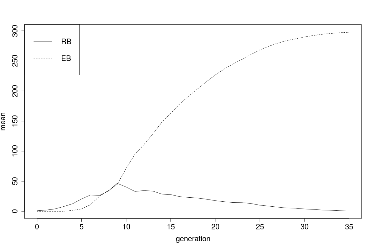
Figure 1: The mean number of EBs and RBs for the death-rate (7) with $C=300$.

For simulations we choose $C=300$. The value function is almost constant 299 with $h(1,0)=298.7$. In Figure 1 we see that the number of RBs is typically small, while the number of EBs starts to increase at an early stage. In Figure 2 there are six trajectories of the process. On Figure 9 (top left) we see the numerical $p$ values. The structure of the death-rate function causes the discontinuity of the $p$ function. Note e.g. that $p(x,y)\equiv 1$ on the line $\{(x,y):2x+y=299\}$, since after one duplication the population reaches the maximum possible value $299$.

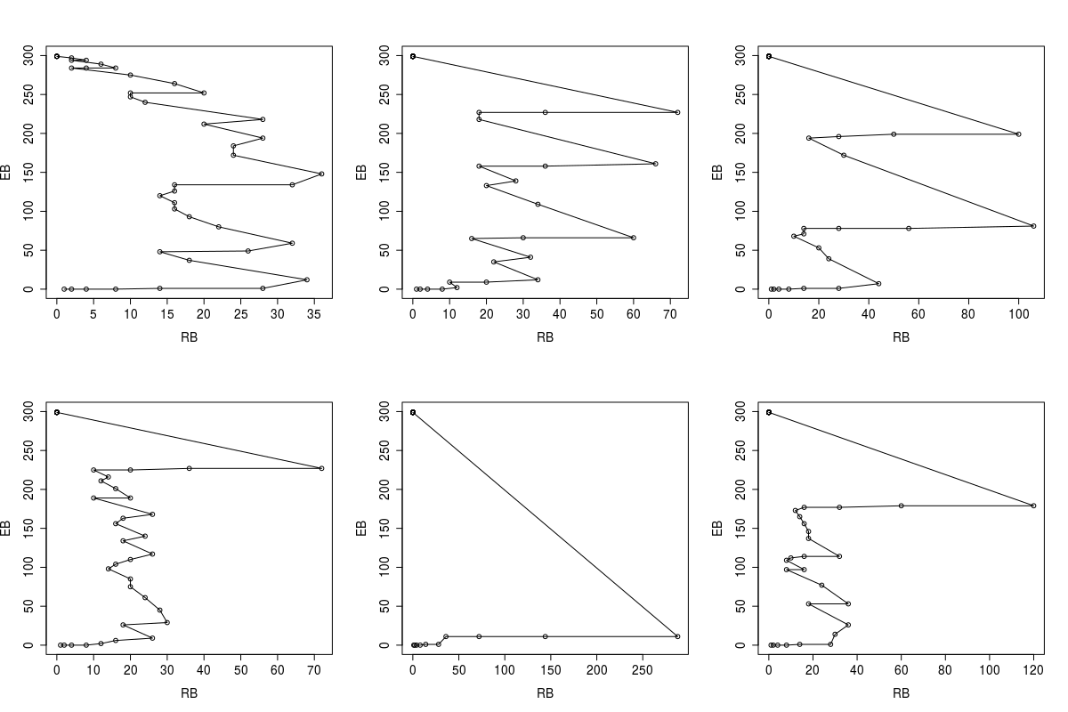
Figure 2: Simulations of the process with death-rate (7) and $C=300$.

Consider a smoother death-rate function

$$d_{2}(x,y)=\begin{cases}1-e^{-c_{0}(\alpha x+\beta y)},&x+y\leq C-1,\\ 1,&x+y\geq C.\end{cases}$$ (8)

If the total number of bacteria is small, then it is unlikely that the host cell dies. The parameters $\alpha,\beta$ allows us to tune the relative effect of EBs and RBs on the host cell’s death. On the one hand RBs are much larger than EBs suggesting $\alpha>\beta$, on the other hand EBs secrete chemicals enhancing cell death. Note that biological experiments suggests that chlamydia controls host cell survival, see [2, p. 392]. We tried three scenarios, with $c_{0}=0.0003$ in each cases and $(\alpha,\beta)=(1,3)$, $(2,2)$, and $(3,1)$, with $C=2500$, $1500$, $3000$, respectively. We chose $C$ large enough, so that the optimal strategy does not depend on its actual value. The rationale of choice of the different threshold values $C$ can be seen from Figure 9. For the empirical mean of 1000 simulations and some typical trajectories see Figures 3 – 8.

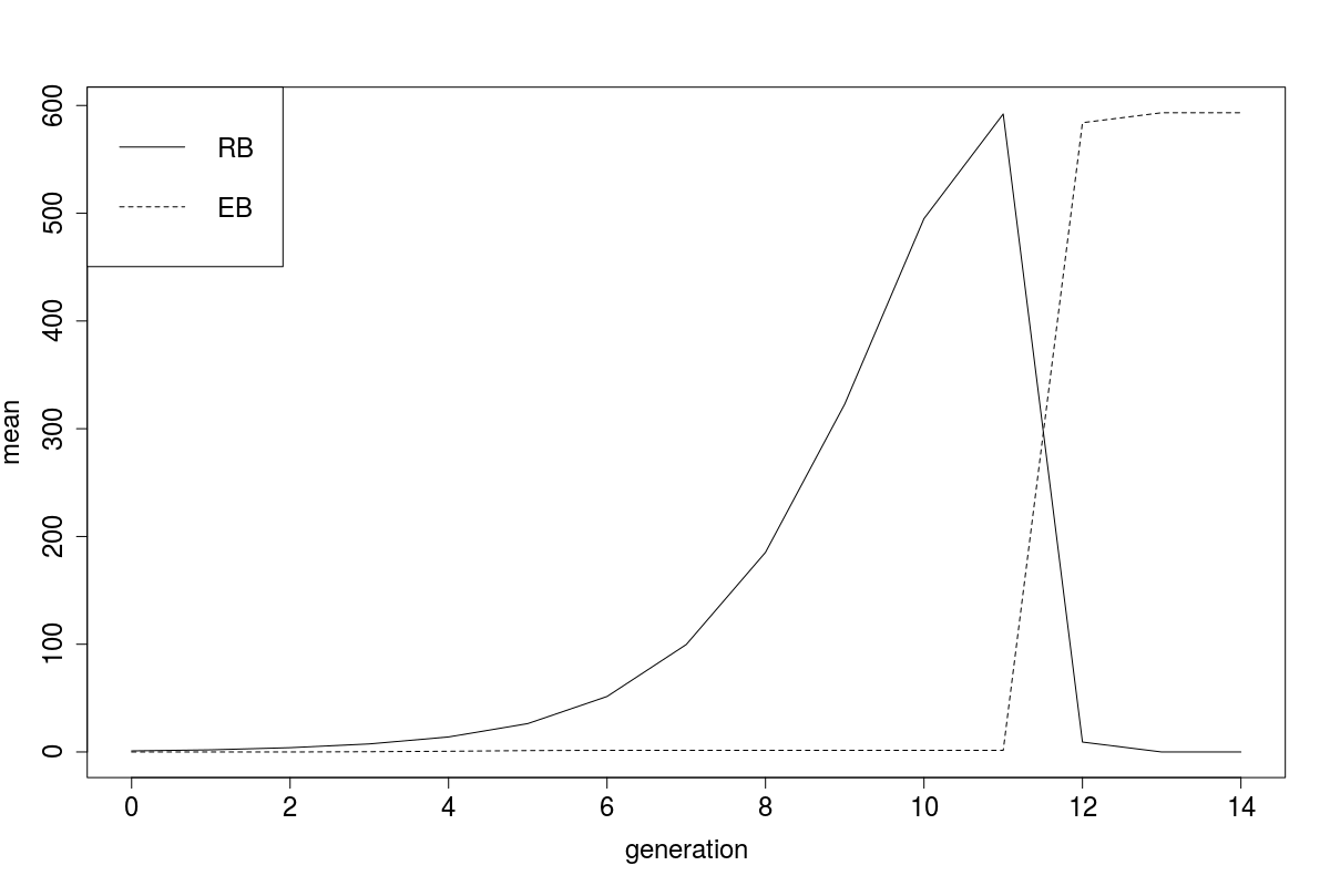
Figure 3: The mean number of EBs and RBs for the death-rate (8), with $(\alpha,\beta)=(1,3)$.

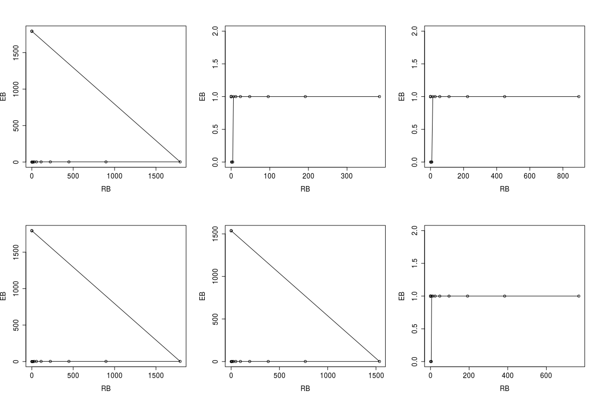
Figure 4: Simulations of the process with death-rate (8), with $(\alpha,\beta)=(1,3)$.

A quick look on the mean functions and on some trajectories of the processes reveals that the population behaves very differently. For $(\alpha,\beta)=(1,3)$ the relative effect of EBs on cell-death is much larger. Therefore, the process prefer to have only RBs up to some point (generation 11), and then all RBs convert to EBs immediately, resulting an ‘all or nothing’ strategy. The exponential increase of RBs and the sudden change is clearly visible both on the means (Figure 3), and on the trajectories (Figure 4). Here $h(1,0)=605$. The optimal $p$ values on Figure 9 (top right) show the same pattern: in each state either all cells duplicate ($p=1$), or all cells convert ($p=0$).

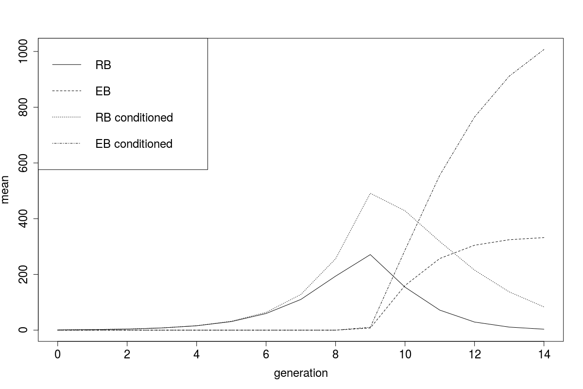
Figure 5: The mean and conditional mean of EBs and RBs for the death-rate (8), with $(\alpha,\beta)=(2,2)$.

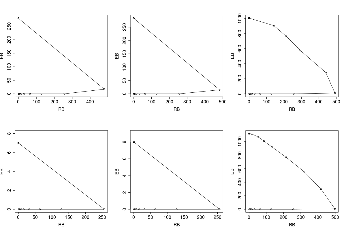
Figure 6: Simulations of the process with death-rate (8), with $(\alpha,\beta)=(2,2)$.

For $(\alpha,\beta)=(2,2)$ the relative effect of RBs and EBs is the same. The RBs duplicate and increase exponentially up to generation 9, then they start to convert to EBs. In Figures 5 and 6 we see that in generations 9–12 the EBs and RBs simultaneously appear, showing the asynchronous conversion obtained in real experiments in [7]. Here $h(1,0)=324$.

gen	0	3	5	7	10	11	12	13
hpi	12	16	20	24	28	32	36	40
RB	1	8	32	128	430	318	213	142
EB	0	0	0	0	287	559	770	910
RB	1.3	7.6	34	105	385	507	271	171
EB	0	0	0	3.7	192	656	706	751

Table 1: Conditional means for $(\alpha,\beta)=(2,2)$ in our simulations, and real data from Lee et al. [7] (last two rows)

In Figure 5 we also plotted the empirical means of the EBs and RBs conditioned on that the host cell is alive. In the real experiment in Lee et al. [7] only those inclusions are counted where the host cell is alive. This clearly causes a bias. We can transform the generation time to real time, hours-post-infection (hpi). After the EB enters the host cell, it takes about 12 hours to convert to RB and to start to duplicate. Between 12 and 24 hpi the doubling time is about 1.8 hours, and around 28 hpi RB-EB conversion starts, see [7, p. 2]. In Table 1 we copied the measurements from [7] to see that our model captures extremely well the experimental data.

For the optimal $p$ values in Figure 9 (bottom left) we do see values other than 0 and 1. There are no big jumps in the $p$ values, which makes it biologically relevant.

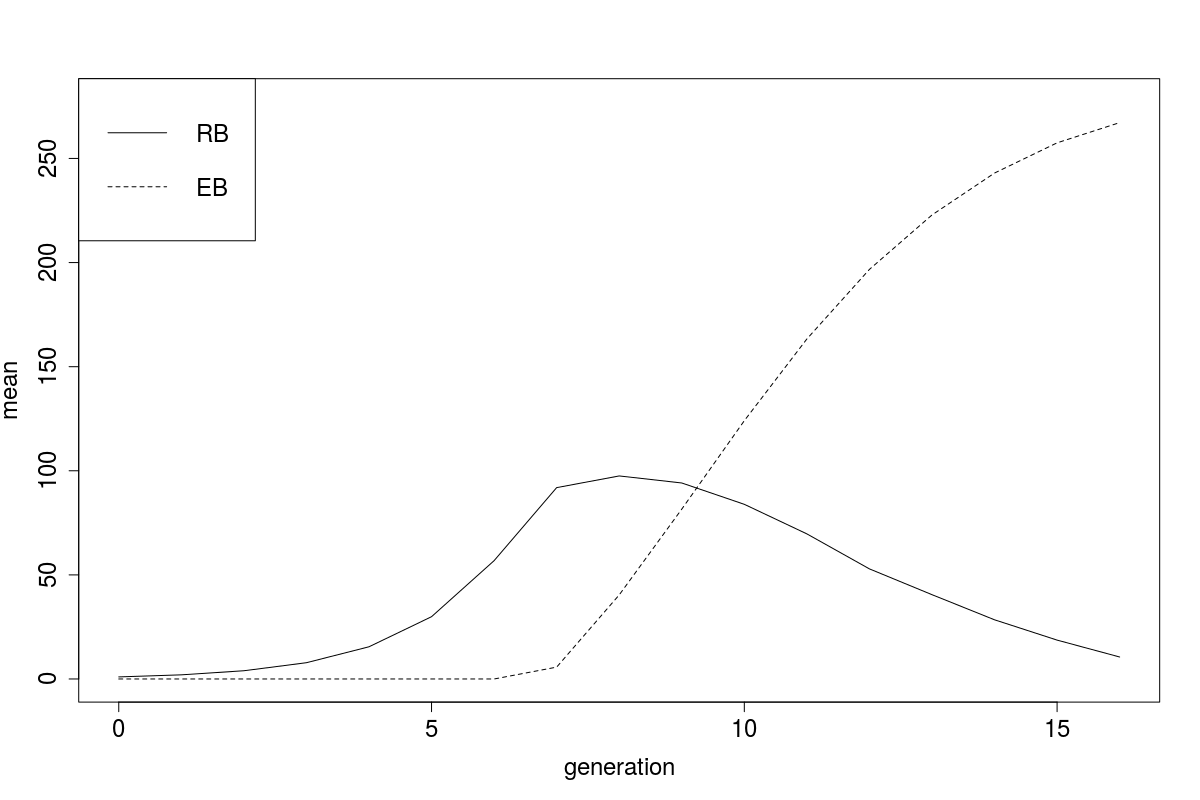
Figure 7: The mean number of EBs and RBs for the death-rate (8), with $(\alpha,\beta)=(3,1)$.

Figure 8: Simulations of the process with death-rate (8), with $(\alpha,\beta)=(3,1)$.

Finally, for $(\alpha,\beta)=(3,1)$ the relative effect of RBs is much larger, which implies a shorter period of exponential increase in the RB population, and a longer coexistence of RB and EB population, see Figures 7 and 8. These results suggest that the effect of RBs on host cell’s death is larger, or at least as large as the effect of EBs. Here $h(1,0)=285.7$. The $p$ values in Figure 9 are even smoother than in the previous case, and the population prefers to have not too many RBs.

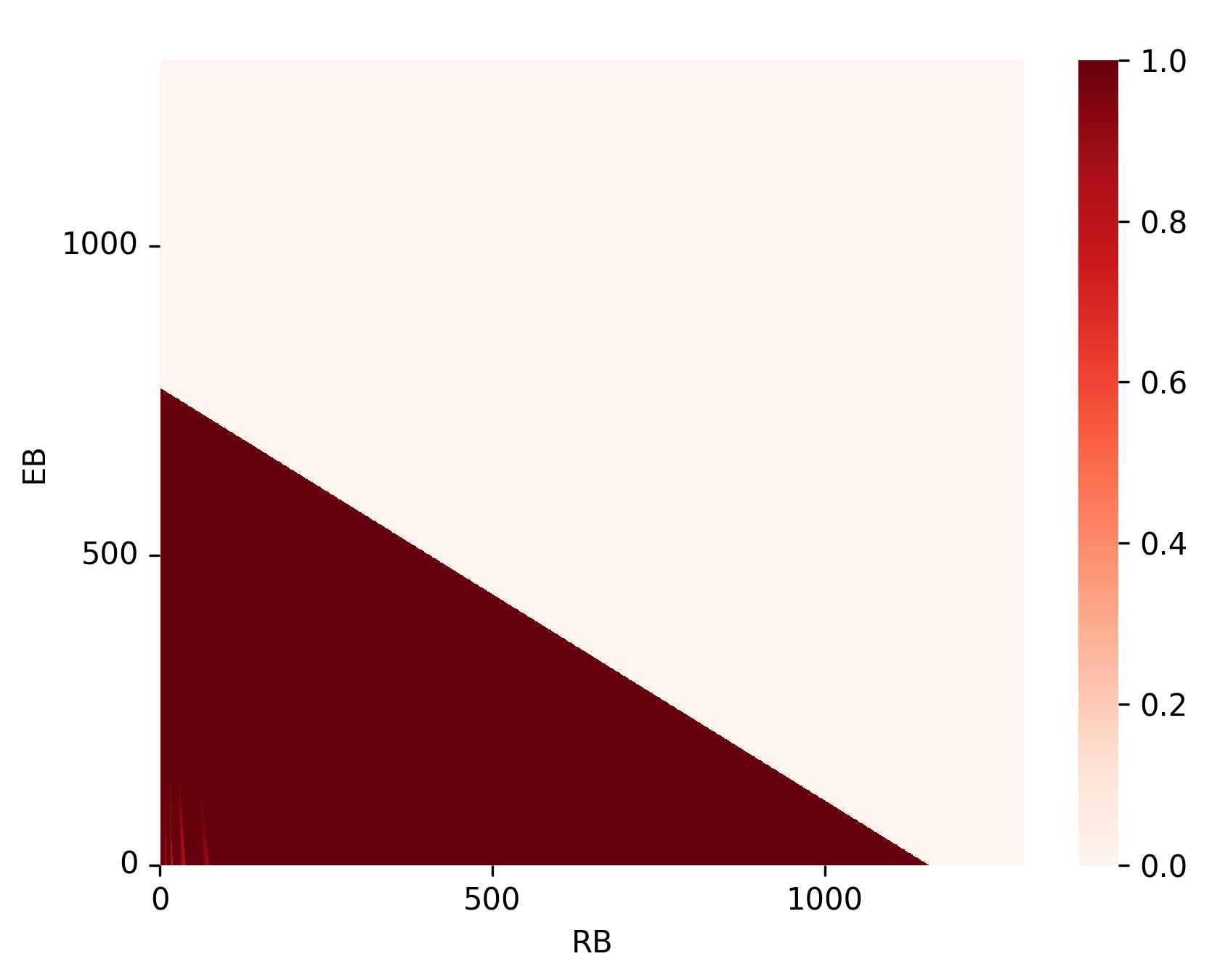
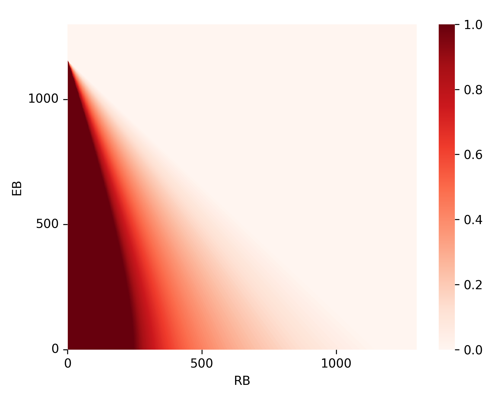
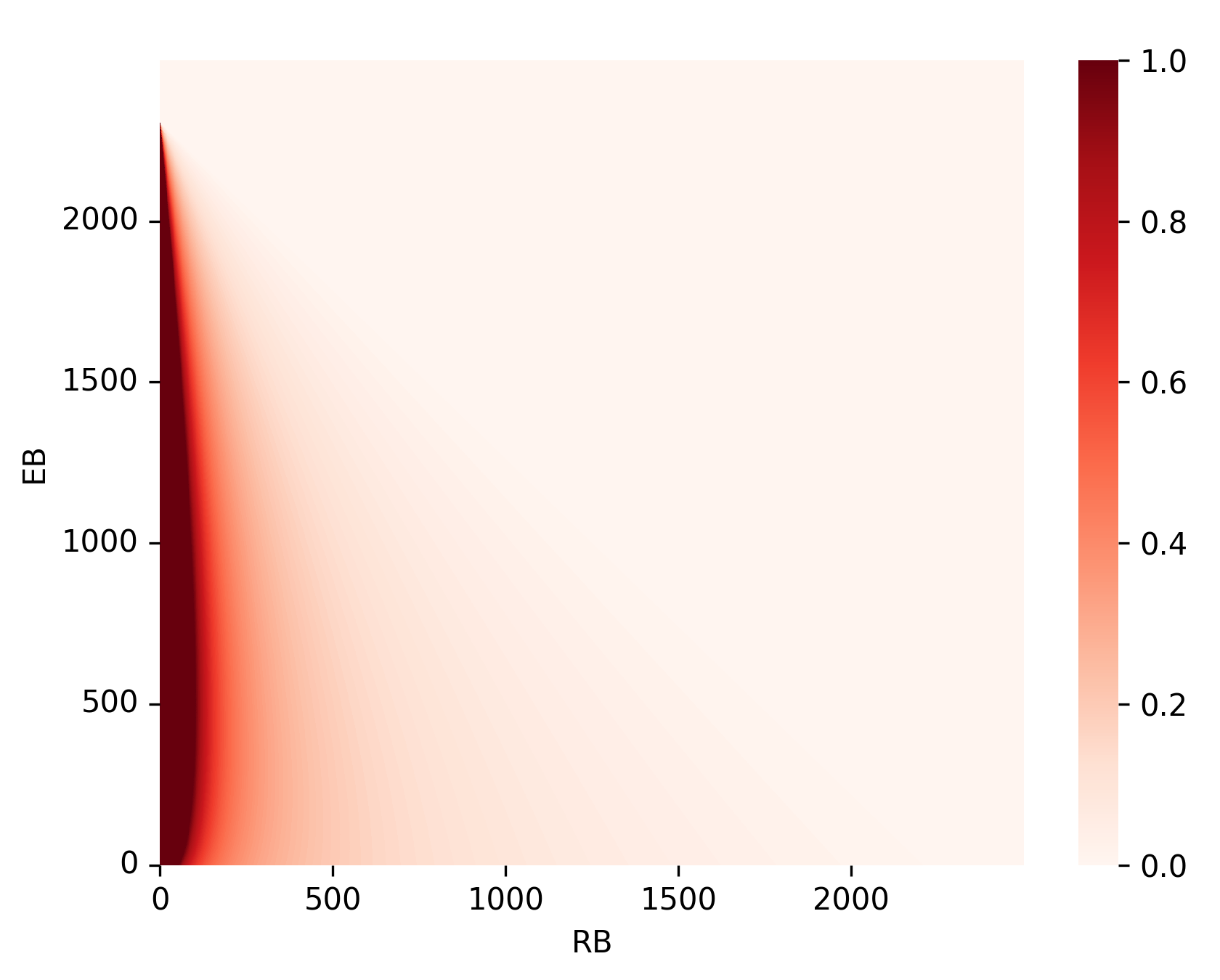
Figure 9: The numerical $p$ values corresponding to the death-rate function (7) with $C=300$ (top left), and to (8) with $(\alpha,\beta)=(1,3)$ (top right), $(\alpha,\beta)=(2,2)$ (bottom left), $(\alpha,\beta)=(3,1)$ (bottom right).

6 Concluding remarks

To model the evolution of Chlamydia populations we propose a novel Galton–Watson branching model, where the state-dependent offspring distribution is determined by solving a stochastic optimization problem. The only input of the process is a death-rate function $d$, which describes the probability that the host cell dies in a given state.

Choosing a natural death-rate function our simulation study shows that the process captures the asynchronous conversion property of the population, which was recently found experimentally in [7]. Moreover, our simulated data fits extremely well to the real measurements in [7], see Table 1. To the best of our knowledge, this is the first mathematical model which reproduces this phenomena.

The cause of the host cell’s death is not yet well-understood. Experiments suggests that chlamydia controls host cell survival, as an early death would be disadvantageous to the bacterial population, see [2, p. 394]. However, the amount of bacteria in the host cell definitely has a strong effect. It is not clear which form of the bacteria is more harmful to the host cell, since RBs are larger physically, while EBs secrete chemicals. Varying the relative effect of RBs and EBs on the death time of the host cell, our simulation studies suggest that RBs and EBs have the same effect on the host cell’s death.

Acknowledgements. We are grateful to Dezső Virok for explaining us the necessary biology. PK is partially supported by the János Bolyai Research Scholarship of the Hungarian Academy of Sciences. MSz is supported by the ÚNKP-22-3-SZTE-457 new national excellence program of the ministry for culture and innovation from the source of the national research, development and innovation fund. This research was supported by the Ministry of Innovation and Technology of Hungary from the National Research, Development and Innovation Fund, project no. TKP2021-NVA-09.

References

- [1] Anita Bogdanov, Péter Kevei, Máté Szalai, and Dezső Virok. Stochastic modeling of in vitro bactericidal potency. Bull. Math. Biol., 84(1):Paper No. 6, 18, 2022.
- [2] C. Elwell, K. Mirrashidi, and J. Engel. Chlamydia cell biology and pathogenesis. Nat Rev Microbiol, 14(24):385–400, 2016.
- [3] German Enciso, Christine Sütterlin, Ming Tan, and Frederic Y. M. Wan. Stochastic chlamydia dynamics and optimal spread. Bull. Math. Biol., 83(4):Paper No. 24, 35, 2021.
- [4] Patsy Haccou, Peter Jagers, and Vladimir A. Vatutin. Branching processes: variation, growth, and extinction of populations, volume 5 of Cambridge Studies in Adaptive Dynamics. Cambridge University Press, Cambridge; IIASA, Laxenburg, 2007.
- [5] Onésimo Hernández-Lerma and Jean Bernard Lasserre. Discrete-time Markov control processes, volume 30 of Applications of Mathematics (New York). Springer-Verlag, New York, 1996.
- [6] Marek Kimmel and David E. Axelrod. Branching processes in biology, volume 19 of Interdisciplinary Applied Mathematics. Springer, New York, second edition, 2015.
- [7] J.K. Lee, G.A. Enciso, D. Boassa, C.N. Chander, T.H. Lou, Pairawan S.S., M.C. Guo, Wan F.Y.M., M.H. Ellisman, C. Sütterlin, and M. Tan. Replication-dependent size reduction precedes differentiation in chlamydia trachomatis. Nat Commun., 45(9):3884–3891, 2018.
- [8] Frederic Y. M. Wan and Germán A. Enciso. Optimal proliferation and differentiation of chlamydia trachomatis. Stud. Appl. Math., 139(1):129–178, 2017.
- [9] D. P. Wilson. Mathematical modelling of chlamydia. ANZIAM J., 45((C)):C201–C214, 2003/04.