A Plaque Test for Redundancies in Relational Data

Abstract.

Inspired by the visualization of dental plaque at the dentist’s office, this article proposes a novel visualization technique for identifying redundancies in relational data. Our approach builds upon an established information-theoretic framework that, despite being well-principled, remains unexplored in practical applications. In this framework, we calculate the information content (or entropy) of each cell in a relation instance, given a set of functional dependencies. The entropy value represents the likelihood of inferring the cell’s value based on the dependencies and the remaining tuples. By highlighting cells with lower entropy, we effectively visualize redundancies in the data. We present an initial prototype implementation and demonstrate that a straightforward approach is insufficient for handling practical problem sizes. To address this limitation, we propose several optimizations, which we prove to be correct. Additionally, we present a Monte Carlo approximation technique with a known error, enabling computationally tractable computations. Using a real-world dataset of modest size, we illustrate the potential of our visualization technique. Our vision is to support domain experts with data profiling and data cleaning tasks, akin to the functionality of a plaque test at the dentist’s.

1. Introduction

Database normalization is a well-studied field, with the theory of functional dependencies as a cornerstone, cf. (Abiteboul et al., 1995). There are several proposals for visualizing functional dependencies, such as sunburst diagrams or graph-based visualizations (Kruse et al., 2017). Yet these approaches only visualize the dependencies, irrespective of the data instance.

We propose a novel visualization that reveals the redundancies captured by functional dependencies. We refer to our approach as a “plaque test”: Like to a dentist who colors dental plaque to show patients unwanted residue on their teeth, our plaque test reveals redundancies in relational data. The plaque test may be applied in data profiling, when dependencies have been discovered, or before carrying out data cleaning tasks or proceeding towards schema normalization — in all these scenarios, domain experts will want to assess the redundancies resident in their data.

Formally, our approach leverages an existing information-theo-retic framework by Arenas and Libkin (Arenas and Libkin, 2003). To the best of our knowledge, we are the first to implement and apply this framework to a practical problem. For better illustration and to provide intuition, we proceed with an illustrative example.

ID	AlbumTitle	Band	BYear	RYear	Track	TrackTitle
1	Not That Kind	Anastacia	1999	2000	1	Not That Kind
1	Not That Kind	Anastacia	1999	2000	2	I’m Outta Love
1	Not That Kind	Anastacia	1999	2000	3	Cowboys …
2	Wish You Were Here	Pink Floyd	1965	1975	1	Shine On You…
3	Freak of Nature	Anastacia	1999	2001	1	Paid my Dues

(a) The relational input data.

ID	AT	B	BY	RY	T	TT
1	0.8	0.8	0.7	0.8	1	1
1	0.8	0.8	0.7	0.8	1	1
1	0.8	0.8	0.7	0.8	1	1
1	1	1	1	1	1	1
1	1	1	0.7	1	1	1

(b) Entropies for only 3 FDs.

ID	AT	B	BY	RY	T	TT
0.6	0.6	0.4	0.4	0.6	1	1
0.6	0.6	0.4	0.4	0.6	1	1
0.6	0.6	0.4	0.4	0.6	1	1
1	1	1	1	1	1	1
1	1	0.7	0.7	1	1	1

(c) Entropies for 23 FDs.

Figure 1. Plaque tests for the original relation (left) with genuine functional dependencies (middle) and automatically discovered functional dependencies (right). Cell color/hue according to entropy values, attribute names abbreviated.

Example 1.1.

Figure 1(a) shows a popular textbook example for discussing database normalization. The relation manages a CD collection. Each CD has an identifier (ID), an AlbumTitle (AT), and was released in a given year (RYear/RY). The band who released the CD (Band/B) was founded in a given year (BYear/BY). Each CD has several tracks (Track/T), each having a title (TrackTitle/TT).

We assume the following functional dependencies to hold:

ID $$\rightarrow\mbox{AlbumTitle, Band, RYear}$$

ID, Track $$\rightarrow\mbox{Title}\qquad\mbox{and}\qquad\mbox{Band}\rightarrow\mbox{BYear}$$

Figure 1(b) shows a plaque test for this relation, given these dependencies: Each cell carries an entropy value, where smaller values reflect a higher degree of redundancy. Accordingly, the deeper the blue hue, the more redundant a value.

Specifically, let us consider the dependency “$\mbox{ID}\rightarrow\mbox{AlbumTitle}$”. In the given instance, the title of the album with ID 1 is recorded redundantly, captured by an entropy of 0.8. If the title were “lost” in the first tuple, it could be recovered from the second or third tuple (and vice versa). In contrast, if the title of Anastacia’s album with ID 3 were lost, it could not be recovered. Intuitively, there is redundancy in the album title “Not That Kind”, which is why it tests positive for redundancy and is highlighted in light blue. This is different for the album title “Freak of Nature”: Cells in white (entropy 1) contain nonredundant data, i.e., their values cannot be recovered from others.

Let us next consider the dependency “Band $\rightarrow$ BYear”, stating that the band determines the year of foundation. Since there are four entries for band Anastacia, the year of foundation is even more redundant than the year of release of her album “Not That Kind”. Accordingly, our plaque test colors the foundation years for Anastacia’s band in a deeper hue (as the entropy drops to 0.7).

So far, we only considered genuine dependencies. We next assume that the dependencies have been automatically discovered in data profiling, yielding additional dependencies.

Example 1.2.

Let us assume that the input relation was profiled by a tool such as Metanome (Papenbrock et al., 2015), which automatically discovers 23 dependencies for this given relation. This includes the cyclic dependency “Band $\rightarrow$ BYear” and “BYear $\rightarrow$ Band”. These happen to hold in the specific instance, but may not hold in general.

Figure 1(c) shows the result of our plaque test. The smaller entropy values, darker hues, and additionally colored cells indicate that the relation now contains additional redundancies. For instance, the entropy value for band Anastacia is as low as 0.4, since it may be recovered from several dependencies, e.g., “ID $\rightarrow$ Band” and “BYear $\rightarrow$ Band”.

As these examples illustrate, the plaque test visually captures redundancies in a way that aligns with intuition.

Contributions

• We apply an existing information-theoretical framework as a “plaque test”, visually revealing redundancies inherent in relational data.

• We show that a straightforward implementation for computing entropy values does not scale beyond toy examples. Accordingly, we propose effective optimizations:

  1. We discuss scenarios where entropy values can be immediately assigned to 1, thereby skipping computation, and where one can focus on a (smaller) subset of the data instance when computing entropy values. We prove the correctness of these optimizations.

  2. We present a Monte Carlo approximation for the computation of entropy values and provide a formula to determine the number of iterations required to achieve a given accuracy with a certain confidence.

• We conduct first experiments with our prototype implementation and present a plaque test on a real-world dataset.

Structure

We give preliminaries on functional dependencies, entropy and information content in Section 2. In Section 3 we introduce two optimizations, one is an exact method and the other an approximate approach. We present our experiments with our prototype in Section 4. We discuss related work in Section 5 and conclude with an outlook in Section 6.

2. Preliminaries

When introducing functional dependencies in Section 2.1, we deviate from the common definition (cf. (Abiteboul et al., 1995)) in that we take the order of tuples into account, allowing us to identify individual cells in a relation instance. The notion of entropy-related information content originates from the work by Arenas and Libkin (Arenas and Libkin, 2003) (Section 2.2). As a first contribution, we then present simplifications to compute the corresponding entropy values (Section 2.3).

Denote by $\mathbb{N}$ the set of positive integers, $\mathbb{N}:=\{1,2,3,\dots\}$.

2.1. Functional Dependencies

Definition 2.1.

A relation $R$ of arity $m$ is specified by a finite set $\operatorname{sort}(R):=\{A_{1},\dots,A_{m}\}$ of attributes $A_{i}$. The domain of an attribute $A$ is denoted by $\operatorname{Dom}(A)$.

An instance $I$ of a relation $R$ is a partial map

$$I\colon\mathbb{N}\rightharpoonup\bigtimes_{A\in\operatorname{sort}(R)}\operatorname{Dom}(A)$$

with finite domain of definition $\operatorname{Def}(I):=\{j\in\mathbb{N}\mid I(j)\text{ is defined}\}$.

The above definition of a relation instance allows duplicate tuples and preserves the order of the tuples.

Definition 2.2.

A relational database schema $S=\{R_{1},\dots,R_{r}\}$ consists of finitely many relations $R_{i}$. Its set of attributes is $\operatorname{sort}(S):=\bigcup_{i}\operatorname{sort}(R_{i})$. An instance $I$ of $S$ consists of an instance $I_{i}$ for each relation $R_{i}$ of $S$.

To simplify the exposition, in this work we consider schemas $S$ consisting of only one relation $R$ and we assume that $\operatorname{Dom}(A)=\mathbb{N}$ for all $A\in\operatorname{sort}(R)$, i.e., each tuple consists of positive integers. Thus an instance $I$ of a relation $R$ of arity $m$ can be seen as just a partial map $I\colon\mathbb{N}\rightharpoonup\mathbb{N}^{m}$.

Definition 2.3.

Let $R$ be a relation and $I$ an instance of $R$. For a subset $K:=\{A_{1},\dots,A_{s}\}\subseteq\operatorname{sort}(R)$ of attributes we have the projection $\pi_{K}(I)$ of the tuples in $I$ to the attributes in $K$. Moreover, for a subset $J\subseteq\operatorname{Def}(I)$ we have the restricted map $I|_{J}\colon J\to\mathbb{N}^{m}$ defined for all indices $j\in J$.

Given an instance $I$ of a relation $R$ we denote by $t_{j}[A_{k}]$ the value of the attribute $A_{k}$ in the $j$-th tuple $t_{j}:=I(j)$ of $I$. Similarly, for a subset $K=\{A_{1},\dots,A_{s}\}\subseteq\operatorname{sort}(R)$ of attributes we denote by $t_{j}[A_{1}\ldots A_{s}]$ the tuple of values $t_{j}[A_{1}],\dots,t_{j}[A_{s}]$, i.e., the $j$-th tuple $\pi_{K}(I(j))$ of the projection $\pi_{K}(I)$.

Definition 2.4.

A functional dependency in a relation $R$ is a pair $f:=(\{A_{1},\dots,A_{s}\},B)$, where $A_{1},\dots,A_{s},B\in\operatorname{sort}(R)$ are attributes. We write such a pair as $A_{1}\ldots A_{s}\to B$.

An instance $I$ of a relation $R$ is said to fulfill the functional dependency $f$ (write $I\models f$) if for all $j_{1},j_{2}\in\operatorname{Def}(I)$ it holds $t_{j_{1}}[A_{1}\ldots A_{s}]=t_{j_{2}}[A_{1}\ldots A_{s}]~{}\Rightarrow~{}t_{j_{1}}[B]=t_{j_{2}}[B]$.

Moreover, the instance $I$ fulfills a set $F$ of functional dependencies (write $I\models F$) if $I\models f$ for all $f\in F$.

We also consider relation instances having unspecified values at some positions. Let $\operatorname{\mathbf{var}}$ be a (countably infinite) set of variables.

Definition 2.5.

Let $I$ be an instance of a relation $R$ with attributes $\operatorname{sort}(R)=\{A_{1},\dots,A_{m}\}$. A position in $I$ is a pair $(j,A_{k})$ with $j\in\operatorname{Def}(I)$ and $k\in\{1,\dots,m\}$; it represents the cell of the $k$-th attribute of the $j$-th tuple, whose value is $t_{j}[A_{k}]$. The instance obtained by putting the value $v$ at position $p=(j,A_{k})$ is denoted by $I_{p\leftarrow v}$.

Let $Q=\{q_{1},\dots,q_{k}\}$ be a set of positions and $X=\{x_{1},\dots,x_{k}\}$ a set of distinct variables. The instance obtained by replacing each position $q_{i}$ by the variable $x_{i}$ for $1\leq i\leq k$ is denoted by $I_{Q\leftarrow X}$ (hence, the instance obtained by replacing the positions from $Q$ by variables, and then position $p$ by the value $v$, is $(I_{Q\leftarrow X})_{p\leftarrow v}$).

An instance $I$ containing distinct variables fulfills a functional dependency $f:=A_{1}\ldots A_{s}\to B$ (write $I\models f$) if for all $j_{1},j_{2}\in\operatorname{Def}(I)$ such that $t_{j_{1}}[B]\notin\operatorname{\mathbf{var}}$ and $t_{j_{2}}[B]\notin\operatorname{\mathbf{var}}$ there holds

$$t_{j_{1}}[A_{1}\ldots A_{s}]=t_{j_{2}}[A_{1}\ldots A_{s}]~{}\Rightarrow~{}t_{j_{1}}[B]=t_{j_{2}}[B].$$

So the above definition requires the functional dependency to be fulfilled only for tuples without variables. Indeed, since all variables are distinct, it is always possible to put in values in their positions such that the functional dependency is fulfilled.

2.2. Entropy and Information Content

In the following we deal with discrete probability spaces $\mathcal{X}=(X,P_{\mathcal{X}})$ on finite sets $X$, where $P_{\mathcal{X}}(x)$ for $x\in X$ denotes the probability of the event $\{x\}$. The information-theoretic entropy of the probability space $\mathcal{X}$ is then given by

$$H(\mathcal{X})\,:=\,-\sum_{x\in X}P_{\mathcal{X}}(x)\log P_{\mathcal{X}}(x).$$

If $\mathcal{A}=(A,P_{\mathcal{A}})$ and $\mathcal{B}=(B,P_{\mathcal{B}})$ are probability spaces on finite sets $A$ and $B$ with joint distribution $P_{\mathcal{A}\times\mathcal{B}}$, then the conditional probability of $a\in A$ given $b\in B$ is defined by

$$P(a|b)\,:=\,\frac{P_{\mathcal{A}\times\mathcal{B}}(a,b)}{P_{\mathcal{B}}(b)}$$

provided that $P_{\mathcal{B}}(b)$ is nonzero. Conversely, the conditional probabilities $P(a|b)$ with the probabilities $P_{\mathcal{B}}(b)$ determine the joint distribution $P_{\mathcal{A}\times\mathcal{B}}$ by the above formula.

Definition 2.6.

Let $\mathcal{A}=(A,P_{\mathcal{A}})$ and $\mathcal{B}=(B,P_{\mathcal{B}})$ be probability spaces. The conditional entropy of $\mathcal{A}$ given $\mathcal{B}$ is

$$H(\mathcal{A}\mid\mathcal{B})\,:=\,-\sum_{b\in B}P_{\mathcal{B}}(b)\sum_{a\in A}P(a|b)\log P(a|b).$$

This value describes the remaining uncertainty in probability space $\mathcal{A}$ given the outcome in $\mathcal{B}$. If the probability distributions of $\mathcal{A}$ and $\mathcal{B}$ are independent, then $P(a|b)=P_{\mathcal{A}}(a)$ for all $b\in B$, and thus $H(\mathcal{A}\mid\mathcal{B})=-\sum_{a\in A}P_{\mathcal{A}}(a)\log P_{\mathcal{A}}(a)=H(\mathcal{A})$.

Consider now a relation instance $I$ of arity $m$ and denote by $\operatorname{Pos}:=\operatorname{Def}(I)\times\{A_{1},\dots,A_{m}\}$ its set of positions. Let $F$ be a set of functional dependencies fulfilled by $I$ and $p\in\operatorname{Pos}$ a position. We define two probability spaces as follows.

First, let $\mathcal{B}(I,p):=(\mathcal{P}(\operatorname{Pos}\setminus\{p\}),P_{\mathcal{B}})$, where $P_{\mathcal{B}}$ is the uniform distribution on the set of all subsets of $\operatorname{Pos}\setminus\{p\}$. This space models the possible cases when we lose a set of possible values from the instance $I$ on positions other than the considered one $p$.

Then, for $k\in\mathbb{N}$ we let $\mathcal{A}_{F}^{k}(I,p):=(\{1,\dots,k\},P_{\mathcal{A}})$, where the conditional probability of $v\in\{1,\dots,k\}$ given $Q\subseteq\operatorname{Pos}\setminus\{p\}$ is

$$P(v|Q)\,:=\,\begin{cases}1/\#V_{Q}&\text{if }v\in V_{Q},\\ 0&\text{otherwise},\end{cases}$$

with $V_{Q}:=\{v\in\{1,\dots,k\}\mid(I_{Q\leftarrow X})_{p\leftarrow v}\models F\}$. This probability space models the possible values in $\{1,\dots,k\}$ to be put in at position $p$ for which we lost the value, when $Q$ is the set of positions of the other lost values in the instance.

Definition 2.7.

Let $F$ be a set of functional dependencies for a schema $S$ and let $I$ be an instance of $S$ with $I\models F$. The information content of position $p$ with respect to $F$ in instance $I$ is given as

$$\operatorname{INF}_{I}(p\mid F)\,:=\,\lim_{k\to\infty}\frac{\operatorname{INF}_{I}^{k}(p\mid F)}{\log k},$$

where $\operatorname{INF}_{I}^{k}(p\mid F):=H(\mathcal{A}_{F}^{k}(I,p)\mid\mathcal{B}(I,p))$ is the conditional entropy of the probability space modelling the possible values for the considered position $p$ given the space modelling the possible sets of other lost values in the instance.

Unfortunately, when using the above formula for the conditional entropy $\operatorname{INF}_{I}^{k}(p\mid F)$ directly, the computation grows exponentially with the number of cells in the given instance. Indeed, for each cell except the one at position $p$ the value can be deleted or not, so every subset of $\operatorname{Pos}\setminus\{p\}$ is an elementary event in the probability space $\mathcal{B}(I,p)$. Therefore, each additional cell in the instance $I$ doubles the number of events to be taken into account for the computation of the information content.

2.3. Simplifications

We now provide more compact and simplified (but still exponentially complex) formulas for the information content. The first result follows easily from the definition of conditional entropy.

Proposition 2.8.

Let $F$ be a set of functional dependencies and $I$ an instance with $I\models F$. Then the information content of a position $p$ in $I$ with respect to $F$ is given by

$$\operatorname{INF}_{I}(p\mid F)=\frac{1}{2^{\#\operatorname{Pos}-1}}\sum_{\!Q\subseteq\operatorname{Pos}\setminus\{p\}\!}\lim_{k\to\infty}\frac{\log\#V_{Q}}{\log k},$$

where $V_{Q}:=\{v\in\{1,\dots,k\}\mid(I_{Q\leftarrow X})_{p\leftarrow v}\models F\}$.

Proof.

By the definition of conditional entropy we obtain

$$\operatorname{INF}_{I}^{k}(p\mid F) =-\sum_{\!Q\subseteq\operatorname{Pos}\setminus\{p\}\!}P_{\mathcal{B}}(Q)\sum_{v=1}^{k}P(v|Q)\log P(v|Q)$$

$$=-\sum_{\!Q\subseteq\operatorname{Pos}\setminus\{p\}\!}\frac{1}{\#\mathcal{P}(\operatorname{Pos}\setminus\{p\})}\sum_{v\in V_{Q}}\frac{1}{\#V_{Q}}\log\frac{1}{\#V_{Q}}$$

$$=\frac{1}{2^{\#\operatorname{Pos}-1}}\sum_{\!Q\subseteq\operatorname{Pos}\setminus\{p\}\!}\log\#V_{Q}.$$

Normalizing and computing the limit shows the assumption. ∎

The values $\operatorname{INF}_{I}(p\mid F,Q):=\lim_{k\to\infty}\frac{\log\#V_{Q}}{\log k}$ can be seen as the information content of $p$ in $I$ with respect to $F$ given a fixed subset $Q\subseteq\operatorname{Pos}\setminus\{p\}$ to be substituted by variables. The next result shows that for these there are only two possible outcomes.

Lemma 2.9.

Let $F$, $I$ and $p$ be as above. For any $Q\subseteq\operatorname{Pos}\setminus\{p\}$ we have $\operatorname{INF}_{I}(p\mid F,Q)\in\{0,1\}$.

Proof.

Consider any “fresh” value $a\in\mathbb{N}$, which does not appear in the column of position $p$ in the relation instance $I$. It is easy to see that whether the instance $(I_{Q\leftarrow X})_{p\leftarrow a}$ fulfills $F$ or not does not depend on the choice of those values $a$. Therefore, either $\log\#V_{Q}/\log k\to 1$ or $\log\#V_{Q}/\log k\to 0$ as $k\to\infty$. ∎

From this lemma and its proof we deduce the following simplification for the computation of information content.

Proposition 2.10.

Let $F$ be a set of functional dependencies and $I$ an instance with $I\models F$. Let $p$ be a position in $I$ with attribute $A$, and let $a\in\mathbb{N}$ be any value not appearing in the column of attribute $A$. Then we have

$$\operatorname{INF}_{I}(p\mid F)=\frac{\#\{Q\subseteq\operatorname{Pos}\setminus\{p\}\mid(I_{Q\leftarrow X})_{p\leftarrow a}\models F\}}{2^{\#\operatorname{Pos}-1}}.$$

Proof.

Define $\mathcal{P}_{a}:=\{Q\subseteq\operatorname{Pos}\setminus\{p\}\mid(I_{Q\leftarrow X})_{p\leftarrow a}\models F\}$. From the proof of the previous lemma we have that $\operatorname{INF}_{I}(p\mid F,Q)=1$ if and only if $Q\in\mathcal{P}_{a}$. Thus we obtain

$$\operatorname{INF}_{I}(p\mid F)=\frac{1}{2^{\#\operatorname{Pos}-1}}\sum_{\!Q\subseteq\operatorname{Pos}\setminus\{p\}\!}\operatorname{INF}_{I}(p\mid F,Q)=\frac{\#\mathcal{P}_{a}}{2^{\#\operatorname{Pos}-1}}.\qed$$

Although we have simplified the computation of the information content somewhat, one needs still to consider all subsets of $\operatorname{Pos}\setminus\{p\}$, leading to exponential complexity. Therefore, we present in the following some optimizations for this computation.

3. Optimizations

In this section we provide optimizations that speed up the computation of information content a lot. In Section 3.1 we deal with exact methods and prove their correctness, while in Section 3.2 we present a very useful approximate approach.

3.1. Reducing the Problem Size

We give two shortcuts for computing the information content in a relation instance. The first identifies positions where there cannot be any redundancy, so that the information content equals $1$.

Definition 3.1.

Let $p=(j,B)\in\operatorname{Pos}$ be a position with attribute $B$ in an instance $I$ and let $f$ be a functional dependency $A_{1}\dots A_{s}\to B$ with $I\models f$. We say that the value at $p$ is unique with respect to $f$ if for every $j^{\prime}\in\operatorname{Def}(I)$ there holds

$$t_{j}[A_{1}\ldots A_{s}]=t_{j^{\prime}}[A_{1}\ldots A_{s}]\,\Rightarrow\,j=j^{\prime}$$

(so if $j\neq j^{\prime}$, then $t_{j}[A_{1}\ldots A_{s}]\neq t_{j^{\prime}}[A_{1}\ldots A_{s}]$).

For a set $F$ of functional dependencies with $I\models F$, the value at $p$ is unique with respect to $F$ if it is unique with respect to all $f\in F$ of the form $A_{1}\ldots A_{s}\to B$.

Note that in particular, a value at position $p$ with attribute $B$ is unique with respect to $F$ in case the attribute $B$ does not appear on the right-hand side of any functional dependency in $F$.

Proposition 3.2.

Let $p\in Pos$ be a position in an instance $I$, where $I\models F$ for a set of functional dependencies $F$. Then $\operatorname{INF}_{I}(p\mid F)=1$ if and only if the value at $p$ is unique with respect to $F$.

Proof.

Let $p=(j,B)\in Pos$ and let $a$ be a “fresh” value not appearing in the column of attribute $B$ in instance $I$.

“$\Leftarrow$”. By Prop. 2.10 it suffices to show that for every subset $Q\subseteq\operatorname{Pos}\setminus\{p\}$ it holds that $(I_{Q\leftarrow X})_{p\leftarrow a}\models F$. So let $f\in F$ be a functional dependency $A_{1}\ldots A_{s}\to B^{\prime}$. From $I\models f$ we know that $I_{Q\leftarrow X}\models f$. Then we have to show that

$$(I_{Q\leftarrow X})_{p\leftarrow a}\models f,$$

i.e., if $t_{j_{1}}[A_{1}\ldots A_{s}]=t_{j_{2}}[A_{1}\ldots A_{s}]$ for some $j_{1},j_{2}\in\operatorname{Def}(I)$ it still holds that $t_{j_{1}}[B^{\prime}]=t_{j_{2}}[B^{\prime}]$, even after inserting value $a$ at position $p$.

Suppose first that $B\neq B^{\prime}$. If $B\notin\{A_{1},\dots,A_{s}\}$ (and $B\neq B^{\prime}$) the assertion above is clear for any value $a$, since the statement is not affected. On the other hand, if $B=A_{i}$ for some $1\leq i\leq s$, then by inserting the fresh value $a$ the hypothesis becomes false, so the statement remains valid.

Now consider the case $B=B^{\prime}$. We may assume that one of $j_{1},j_{2}$ equals the index $j$ of position $p$ and write $j^{\prime}$ for the other index. Then if $t_{j}[A_{1}\ldots A_{s}]=t_{j^{\prime}}[A_{1}\ldots A_{s}]$, it follows from the uniqueness property that $j=j^{\prime}$. So the above statement still holds after inserting the value $a$, since the tuple indices coincide.

“$\Rightarrow$”. Suppose the value at $p$ is not unique with respect to $F$. Then there is a functional dependency $A_{1}\dots A_{s}\to B$ in $F$ such that $t_{j}[A_{1}\ldots A_{s}]=t_{j^{\prime}}[A_{1}\ldots A_{s}]$ for an index $j^{\prime}$ distinct from the index $j$ of position $p$. However, considering $Q:=\varnothing$ this functional dependency is not fulfilled anymore by the instance $(I_{Q\leftarrow X})_{p\leftarrow a}=I_{p\leftarrow a}$. Indeed, as the value $a$ does not appear in the column of attribute $B$, we have $t_{j}[B]\neq t_{j^{\prime}}[B]$ after the insertion. This shows that $\operatorname{INF}_{I}(p\mid F)<1$ by Prop. 2.10. ∎

In the second optimization we reduce the considered instance to the relevant tuples and attributes. This may shrink the number of cells and thus decrease the runtime exponentially. After performing this step we can apply the first shortcut in the smaller table and use the outcome for the original instance.

Let $I$ be a relation instance of arity $m$ and let $J\subseteq\operatorname{Def}(I)$, $K\subseteq\{A_{1},\dots,A_{m}\}$ where the $A_{k}$ are the attributes of the relation. The subinstance $I(J,K)$ consists of all tuples of the projection $\pi_{K}(I)$ with index $j\in J$. We also let $\operatorname{Pos}(J,K):=J\times K\subseteq\operatorname{Pos}$ be the corresponding set of positions.

Proposition 3.3.

Let $F$ be a set of functional dependencies and $I$ an instance with $I\models F$. Denote by $J_{0}$ the set of all indices $j_{0}\in\operatorname{Def}(I)$ such that for some position $p=(j_{0},A_{k})\in\operatorname{Pos}$ the value at $p$ is not unique with respect to $F$. Denote by $K_{0}$ the union of all attributes $\{A_{1},\dots,A_{s},B\}$ involved in any functional dependency $A_{1}\dots A_{s}\to B$ in $F$. Then for every $J\supseteq J_{0}$ and $K\supseteq K_{0}$ there holds

$$\forall p\in\operatorname{Pos}(J,K)\colon\operatorname{INF}_{I}(p\mid F)=\operatorname{INF}_{I(J,K)}(p\mid F).$$

Proof.

Write $I^{\prime}:=I(J,K)$ and $\operatorname{Pos}^{\prime}:=\operatorname{Pos}(J,K)$. Let $p=(j,B)\in\operatorname{Pos}^{\prime}$ be a position in the subtable and let $a$ be a “fresh” value not appearing in the column of attribute $B$ in the whole instance $I$. Consider a functional dependency $f\colon A_{1}\ldots A_{s}\to B$ in $F$, as well as subsets $Q^{\prime}\subseteq\operatorname{Pos}^{\prime}\setminus\{p\}$ and $Q\subseteq\operatorname{Pos}\setminus\{p\}$ such that $Q\cap\operatorname{Pos}^{\prime}=Q^{\prime}$. We claim that

$$(I^{\prime}_{Q^{\prime}\leftarrow X})_{p\leftarrow a}\models f\quad\Leftrightarrow\quad(I_{Q\leftarrow X})_{p\leftarrow a}\models f\,.$$

Indeed, suppose that $t_{j}[A_{1}\ldots A_{s}]=t_{j^{\prime}}[A_{1}\dots A_{s}]$ for some $j,j^{\prime}\in\operatorname{Def}(I)$ in instance $(I_{Q\leftarrow X})_{p\leftarrow a}$. If both $j,j^{\prime}\in J$ this implies $t_{j}[B]=t_{j^{\prime}}[B]$ since $(I^{\prime}_{Q^{\prime}\leftarrow X})_{p\leftarrow a}$ fulfills $f$. In the other case, at least one index is not in $J$, say $j$. By assumption, the value of the $j$-th tuple at attribute $B$ is unique with respect to $f$, hence it follows that $j=j^{\prime}$ and thus $t_{j}[B]=t_{j^{\prime}}[B]$. The converse direction is clear.

Let $r:=\#\operatorname{Pos}$ and $r^{\prime}:=\#\operatorname{Pos}^{\prime}$. Given $Q^{\prime}\subseteq\operatorname{Pos}^{\prime}\setminus\{p\}$ it is easy to see that the number of $Q\subseteq\operatorname{Pos}\setminus\{p\}$ such that $Q\cap\operatorname{Pos}^{\prime}=Q^{\prime}$ equals $2^{r-r^{\prime}}$ (one adjoins a subset in $\operatorname{Pos}\setminus\operatorname{Pos}^{\prime}$). Then letting $\mathcal{P}_{a}:=\{Q\subseteq\operatorname{Pos}\setminus\{p\}\mid(I_{Q\leftarrow X})_{p\leftarrow a}\models F\}$ and $\mathcal{P}^{\prime}_{a}:=\{Q^{\prime}\subseteq\operatorname{Pos}^{\prime}\setminus\{p\}\mid(I^{\prime}_{Q^{\prime}\leftarrow X})_{p\leftarrow a}\models F\}$, we deduce from these observations that

$$2^{r-r^{\prime}}\#\mathcal{P}^{\prime}_{a}=\#\mathcal{P}_{a}\,.$$

Therefore, using Prop. 2.10 it follows that

$$\operatorname{INF}_{I}(p\mid F)=\frac{\#\mathcal{P}_{a}}{2^{r-1}}=\frac{2^{r-r^{\prime}}\#\mathcal{P}^{\prime}_{a}}{2^{r-1}}=\frac{\#\mathcal{P}^{\prime}_{a}}{2^{r^{\prime}-1}}=\operatorname{INF}_{I^{\prime}}(p\mid F).\qed$$

Example 3.4.

Consider the instance

A	B	C	D
7	2	8	4
5	2	8	6
7	2	8	6

and the set of functional dependencies $F:=\{\text{A}\to\text{C}\}$.

Since the attributes A, B or D do not appear on the right-hand side of the functional dependency, Prop. 3.2 implies that $\operatorname{INF}_{I}(p\mid F)=1$ for all $p=(j,A_{k})$ with $A_{k}\neq\text{C}$. Additionally, by Prop. 3.2 we obtain that $\operatorname{INF}_{I}((2,\text{C})\mid F)=1$, since the value at position $p=(2,\text{C})$ is unique with respect to $F$.

We can reduce the table using Prop. 3.3 by removing the second tuple and the attributes B and D. The resulting subtable is

A	C
7	8
7	8

for which the number of subsets in $\operatorname{Pos}(J,K)\setminus\{p\}$ is reduced from $2^{15}$ to $2^{3}$, i.e., by a factor over 4’000.

Consider position $p=(1,\text{C})$ and the subsets $Q\subseteq\operatorname{Pos}(J,K)\setminus\{p\}$. For $Q=\varnothing$, i.e., the values in all positions different from $(1,\text{C})$ are present, the instance $(I_{Q\leftarrow X})_{p\leftarrow v}=I_{p\leftarrow v}$ fulfills the functional dependency $\text{A}\to\text{C}$ only if $v=8$. For all other subsets $Q$, i.e., at least one more value is lost, we obtain $(I_{Q\leftarrow X})_{p\leftarrow v}\models F$ for all values $v$. Therefore $\operatorname{INF}_{I}(p\mid F)=\frac{7}{8}=0.875$. The computation of $\operatorname{INF}((3,\text{C})\mid F)$ is similar, and we get the result

$$\big{(}\operatorname{INF}_{I}((j,A_{k})\mid F)\big{)}=\begin{pmatrix}1&1&0.875&1\\ 1&1&1&1\\ 1&1&0.875&1\end{pmatrix}.$$

3.2. Monte Carlo Approximation

Despite the aforementioned optimizations the computation of information content may be practically out of reach, even in relation instances of moderate size. This may be the case in particular if the prerequisites for applying the shortcuts are not given. A workaround for these cases can be a probably good approximation. This approach can also be combined with the two shortcuts, e.g., by identifying cells with full information content first, then reducing the problem to a smaller subtable (if possible) and finally computing the values on this subtable with an approximation algorithm.

The approximation is computed with a randomized algorithm, the Monte Carlo method, as introduced in Chapter 11 of (Mitzenmacher and Upfal, 2017). Instead of considering all subsets of positions (minus the considered one), we pick a sample of subsets uniformly at random and take the average of the corresponding results. The following tool is deduced from Theorem 4.14 of (Mitzenmacher and Upfal, 2017) and useful for estimating the accuracy of this method.

Proposition 3.5 (Hoeffding’s inequality).

Let $X_{1},\dots,X_{n}$ be independent identically distributed random variables such that$a_{i}\leq X_{i}-\operatorname{E}[X_{i}]\leq b_{i}$. Then for any $c>0$ it holds

$$\Pr\Big{(}\textstyle\sum\limits_{i=1}^{n}(X_{i}-\operatorname{E}[X_{i}])\geq c\Big{)}\leq\exp\Big{(}\dfrac{-2c^{2}}{\sum_{i=1}^{n}(b_{i}-a_{i})^{2}}\Big{)}.$$

In order to approximate the information content we consider the probability space $\mathcal{B}(I,p):=(\mathcal{P}(\operatorname{Pos}\setminus\{p\},P_{\mathcal{B}})$ from Section 2 with uniform distribution $P_{\mathcal{B}}$. Define random variables

$$X_{i}\colon\mathcal{P}(\operatorname{Pos}\setminus\{p\})\to[0,1],\quad Q\mapsto\lim_{k\to\infty}\frac{\log\#V_{Q}}{\log k},$$

with $V_{Q}:=\{v\in\{1,\dots,k\}\mid(I_{Q\leftarrow X})_{p\leftarrow v}\models F\}$. Then by Prop. 2.10 there holds $\operatorname{E}[X_{i}]=\operatorname{INF}_{I}(p\mid F)$. This motivates the next theorem about the randomized approach to compute the information content with accuracy $\varepsilon$ and confidence $1\!-\!\delta$.

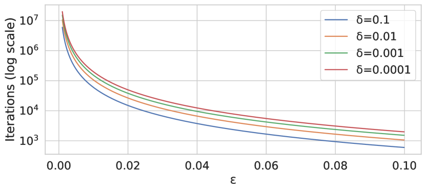
Figure 2. Required iterations to achieve an accuracy ($\varepsilon$) with a certain confidence ($1\!-\!\delta$) in Monte Carlo approximation.

Theorem 3.6.

Let $p\in\operatorname{Pos}$ be a position in a relation instance $I$, where $I\models F$ for a set $F$ of functional dependencies. Let $X_{1},\dots,X_{n}$ be independent identically distributed random variables as above and $X:=\frac{1}{n}\sum_{i=1}^{n}X_{i}$ their average. Then for all $\varepsilon,\delta>0$ there holds

$$\Pr\big{(}|X-\operatorname{INF}_{I}(p\mid F)|\geq\varepsilon\big{)}\leq\delta$$

provided that $n\geq 2\ln(2/\delta)/\varepsilon^{2}$.

Proof.

Since $0\leq X_{i}\leq 1$ we have $-1\leq X_{i}-\operatorname{E}[X_{i}]\leq 1$, so by applying Hoeffding’s inequality with $\sum_{i=1}^{n}(b_{i}-a_{i})^{2}=4n$ we find the upper bound $\exp(-n\varepsilon^{2}/2)$ for $\Pr(\sum_{i=1}^{n}(X_{i}-\operatorname{E}[X_{i}])\geq n\varepsilon)$, so that $\Pr(|X-\operatorname{E}[X_{i}]|\geq\varepsilon)\leq 2\exp(-n\varepsilon^{2}/2)\leq\delta$. ∎

Example 3.7.

Assume that for the approximation of information content for an instance $I$ at position $p$ with respect to $F$, we allow an error of at most $0.001$ with probability at least $99.9\%$. This can be realized by sampling $Q\subseteq\operatorname{Pos}\setminus\{p\}$ and computing $X_{i}(Q)$ at least $2\ln(2/10^{-3})/(10^{-3})^{2}\geq 1.52\!\cdot\!10^{7}$ times.

If a less exact approximation is sufficient, say with an error of at most $0.01$ with the same probability as before, then the required number of runs are lowered by a factor $100$, thus only $1.52\!\cdot\!10^{5}$ samples are necessary.

Figure 2 show a plot of the required iterations to achieve a certain accuracy ($\varepsilon$) with a certain confidence ($1-\delta$). For instance, to achieve an accuracy of 0.04 with a confidence of 99.9% ($1-\delta$) we need, around 10 000 iterations.

4. Experiments

Our experiments target the following research questions:

RQ1:

Is the plaque test informative for real-world datasets?

RQ2:

Can we afford to compute exact entropy values or do we need to resort to Monte Carlo approximation?

RQ3:

How does the runtime of the Monte Carlo approximation scale with the number of iterations?

Below, we report on our insights with a first prototype implementation and using moderate-sized but real-world datasets.

Implementation

We implemented our algorithm as a single-threaded Java implementation. Our dispatcher is a Python script which also measures the end-to-end runtime of the Java program.

Datasets

We explore redundancies in a dataset on natural satellites from the WDC Web Table Corpus. From this data, the dependency discovery tool Metanome (Papenbrock et al., 2015) discovers 35 left-reduced functional dependencies with a single attribute on the right, which we use in our experiments. We use additional datasets in Figure 3: Iris, with 4 functional dependencies, Adult with 78 functional dependencies, Echocardiogram with 538 functional dependencies and NCVoter with 758 functional dependencies. To retrieve the functional dependencies, we again employ Metanome.

For the datasets Satellites, Adult, Iris and NCVoter, we only use an excerpt, containing the first 150 rows. For Echocardiogram, we use all 132 rows of the dataset.

Environment

We use an Intel Xeon Gold 6242R (3.1 GHz) CPU and 192GB of RAM, running Ubuntu 22.04 and Java 18.

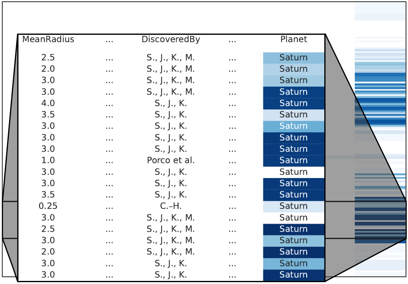
(a) Satellites (150) Min: 0.61

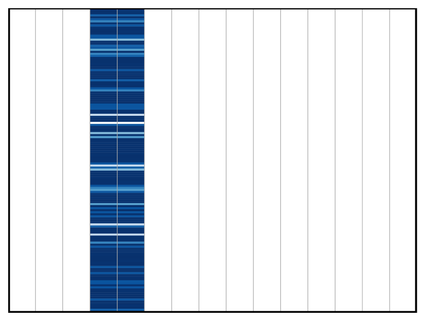
(b) Adult (150) Min: 0.50

(c) Iris (150) Min: 0.95

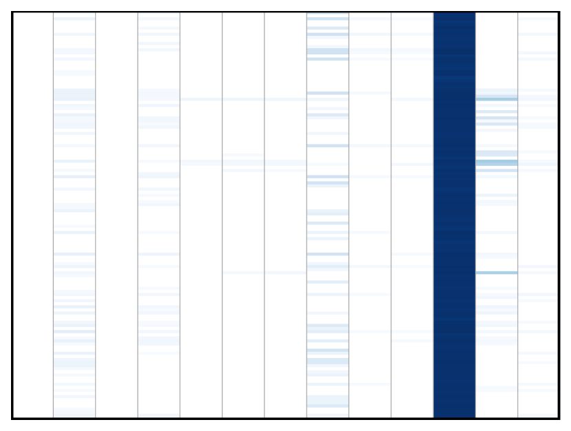
(d) Echocard. (132) Min: 0.00

(e) NCVoter (150) Min: 0.00

Figure 3. Visual “plaque test”: Color-coded entropy values for different datasets. Sub-captions declare numbers of rows in parentheses and minimum entropy values, rounded to the second decimal place. Colors scaled individually, w.r.t. the minimum entropy value. For (a), a zoom-in on an excerpt of the data is superimposed.

We now address the research questions in turn.

RQ1

We perform the plaque test for the satellite, adult, echocardiogram, iris and NCVoter dataset, and show the visual plaque tests in Figure 3. Cells with an entropy value of 1 are shown in white and cells with values below 1 are colored in shades of blue, with darker shades indicating lower values. The color scales are calibrated individually for each dataset, i.e., colors from different datasets can not be compared. The entropy values are computed with Monte Carlo simulation at 100’000 iterations, with an accuracy of approx. 0.01 and a confidence of 99%.

We next discuss the datasets individually, and focus on the Satellite dataset in particular detail.

Satellites. In Figure 3(a), we see the first 150 rows of the satellite dataset. Only the last column, “Planet”, and very few cells in the second-to-last column, “Notes”, have entropy values below 1. We zoom in on a subset of the rows, hiding only cells with an entropy value of 1, and showing the values of the columns “MeanRadius”, “DiscoveredBy” and “Planet”. The excerpt hints at a connection between values in “MeanRadius” and the entropy of “Planet”: for tuples with a mean radius of 3.0, the entropy of the planet is the lowest. Indeed, “MeanRadius” is on the left-hand side of numerous functional dependencies, including $MeanRadius,DiscoverdBy\to Planet$ and a value of 3.0 only occurs for satellites of Saturn. Hence, “MeanRadius” should intuitively be a good indicator of the entropy of “Planet”. Thus, we can explain lower entropy values (or the “plaque”), as well as entropy values of 1, which we take as a sign that the visualization is effective.

In Figure 3(a), the majority of cells has entropy 1. Figure 4 shows a histogram of the entropy values, to provide more insight into their distribution. Among a total of 1.200 cells, approx. 80% have an entropy value of 1. Values below 1 are scarce, with the lowest value being close to 0.6. Overall, the information content of the cells is rather high and only around 5% of the cells have an entropy value below 0.9. The high number of cells with entropy 1 shows that the optimizations introduced in Section 3 effectively reduce the problem size.

Adult. In Figure 3(b), only two columns, “education” and “education-num” have entropy values below 1. For each row, both columns have the same entropy value because the functional dependencies “$\text{education}\to\text{education-num}$” and “$\text{education-num}\to\text{education}$” hold. This means that “education” uniquely identifies “education-num” and vice versa.

Iris. In the Iris dataset (Figure 3(c)), there are only FDs with the last column, “class”, on the right side. Consequently, only this column has entropy values below 1.

Echocardiogram and NCVoter. The datasets in Figures 3(d) and 3(e) exhibit the lowest minimum entropy values, as both have a column with a single-valued domain. Moreover, the two datasets have the highest number of columns with entropy values below 1. In Echocardiogram, 11 out of 13 columns contain entropies below 1 and in NCVoter, 15 out of 19 columns have entropies below 1.

Results. Our visual plaque tests, applied to five standard datasets in dependency discovery, shows promising results: When “plaque” is detected, it aligns with intuition as we can provide an explanation by examining the functional dependencies and the corresponding cell values. Moreover, on the real world datasets shown, the plaque test is rather selective, testing positive for only a small share of cells (and in fact, concentrates on a few attributes). This can be a further indicator that the visualization is consumable for humans.

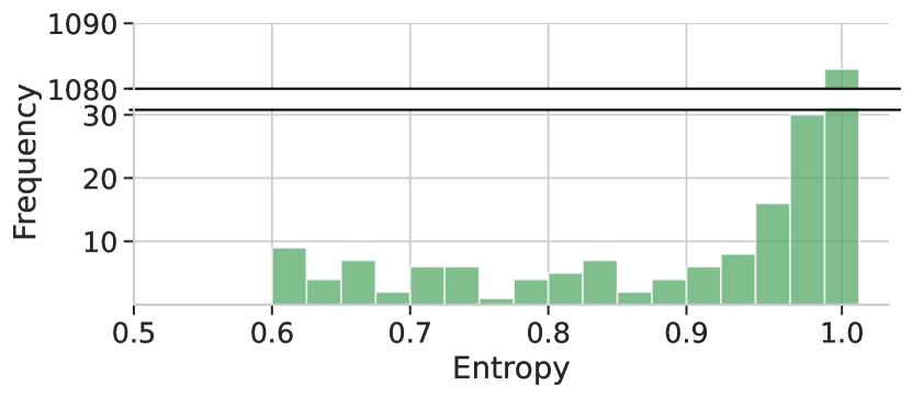
Figure 4. Histogram over entropy values in the first 150 rows of the satellites dataset (accuracy: 0.01, 99.9% confidence).

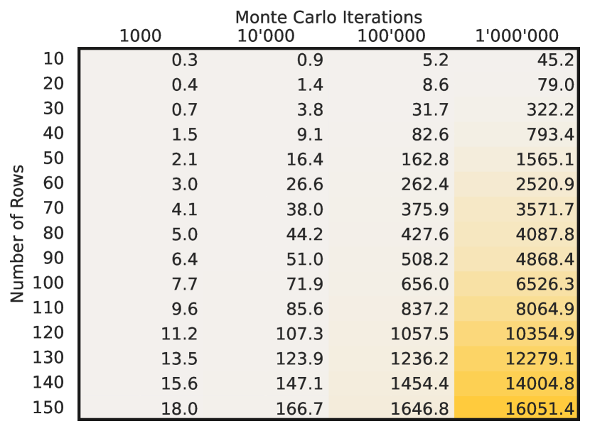
Figure 5. Runtime in seconds on the satellite dataset, for different numbers of Monte Carlo iterations and subset sizes of the data. Higher saturation indicates longer runtimes.

RQ2

Table 1 shows the runtime in seconds for computing the exact entropy values on different subsets of the satellite data. We compare the algorithm with the optimizations from Section 3 disabled/enabled. Note that we are computing exact entropies, without Monte Carlo approximation.

#R	Unoptimized	Optimized
1	0.128	0.097
2	1.318	0.099
3	461.059	0.320
4	-	0.355
5	-	25’221.186
6	-	-

Table 1. Runtime in seconds for computing exact entropy values without/with the optimizations from Section 3. “#R” states cardinality of input relation. Runs marked “-” aborted after 24 hours.

The unoptimized algorithm can process only up to three rows within 24 hours. Using the optimizations, up to five rows could be computed within 24 hours.

Results. While we can show our optimizations to be effective compared to the unoptimized implementation, computing the exact entropies remains prohibitively expensive for anything but textbook or toy examples. we proceed with exploring the runtimes of Monte Carlo approximation.

RQ3

We next explore the runtimes of the Monte Carlo approximation. As visualized in Figure 2, users can control the accuracy and confidence of the approximation result by the number of Monte Carlo iterations.

In Figure 5, the elapsed runtimes in seconds for different subsets of the satellite data and different numbers of Monte Carlo iterations are shown.

For reasonably large subsets, runtime scales linearly with the number of iterations while the input size influences runtime more heavily. While calculating the entropy for 150 rows takes around 4.5 hours at 1’000’000 iterations, we already have an accuracy of approx. 0.01 with 99% confidence at 100’000 iterations (see Figure 2), which takes around 30 minutes to calculate.

Results. With Monte Carlo approximation, we can achieve reasonable runtimes, while being in control of the parameters accuracy and confidence. However, to scale to larger inputs, further research and engineering efforts are required. We point out ideas for future optimizations as part of our outlook in Section 6.

5. Related Work

Functional Dependencies

Dependency discovery is an established and active field, and we refer to (Abedjan et al., 2018) for an overview. Visualizing dependencies is not as well studied, and existing approaches such as sunburst diagrams or graph-based visualizations (Kruse et al., 2017) do not take the data instance into account. In contrast, our plaque test does not visualize the dependencies per se, but the redundancies captured by them in the data instance.

Our visualization leverages heat maps imposed over relational data. This idea has been explored in a different context, such as visualizing the frequency of changes to the data instance (Bleifuß et al., 2019).

Information Theory and Databases

We build upon an information-theoretic framework developed by Arenas and Libkin (Arenas and Libkin, 2003), which allows to justify the classic normalization into normal forms and to propose a well-grounded normal form for XML.

In an orthogonal effort, Lee (Lee, 1987) proposed entropies on the instance-level which is not tied to a set of functional dependencies. Therefore, it does not lend itself to the plaque test as proposed by us.

More recently, information theory has also been investigated within database theory research in the context of deciding query containment, e.g., (Abo Khamis et al., 2020).

6. Outlook

We have proposed a visual plaque test to reveal redundancies in relational data, based on functional dependencies.

In our experiments with our first prototype, we work with rather small datasets. Scaling to larger datasets is part of future work, and we see several possibilities for optimizing the runtime, like parallelization or linear programming techniques.

Once we are able to scale to larger datasets, we will need to address the consumability of our visualization. For instance, we may allow users to interactively cluster cells with plaque, for easy browsing and inspection. We may also explore the impact of individual dependencies by excluding them ad-hoc from the visualization. This raises the question of whether the entropy values can be computed incrementally, based on a fluctuating set of functional dependencies.

We also plan to investigate the visualization of further kinds of dependencies, such as join dependencies and multi-valued dependencies, since they are also covered by the underlying information-theoretic framework.

- (1)
- Abedjan et al. (2018) Ziawasch Abedjan, Lukasz Golab, Felix Naumann, and Thorsten Papenbrock. 2018. Data Profiling. Morgan & Claypool Publishers. https://doi.org/10.2200/S00878ED1V01Y201810DTM052
- Abiteboul et al. (1995) Serge Abiteboul, Richard Hull, and Victor Vianu. 1995. Foundations of Databases. Addison-Wesley. http://webdam.inria.fr/Alice/
- Abo Khamis et al. (2020) Mahmoud Abo Khamis, Phokion G. Kolaitis, Hung Q. Ngo, and Dan Suciu. 2020. Bag Query Containment and Information Theory. In Proc. PODS. 95–112. https://doi.org/10.1145/3375395.3387645
- Arenas and Libkin (2003) Marcelo Arenas and Leonid Libkin. 2003. An information-theoretic approach to normal forms for relational and XML data. In Proc. PODS. 15–26. https://doi.org/10.1145/773153.773155
- Bleifuß et al. (2019) Tobias Bleifuß, Leon Bornemann, Dmitri V. Kalashnikov, Felix Naumann, and Divesh Srivastava. 2019. DBChEx: Interactive Exploration of Data and Schema Change. In Proc. CIDR. http://cidrdb.org/cidr2019/papers/p65-bleifuss-cidr19.pdf
- Kruse et al. (2017) Sebastian Kruse, David Hahn, Marius Walter, and Felix Naumann. 2017. Metacrate: Organize and Analyze Millions of Data Profiles. In Proc. CIKM. 2483–2486. https://doi.org/10.1145/3132847.3133180
- Lee (1987) T.T. Lee. 1987. An Information-Theoretic Analysis of Relational Databases—Part I: Data Dependencies and Information Metric. IEEE Transactions on Software Engineering SE-13, 10 (1987), 1049–1061. https://doi.org/10.1109/TSE.1987.232847
- Mitzenmacher and Upfal (2017) M. Mitzenmacher and E. Upfal. 2017. Probability and Computing: Randomization and Probabilistic Techniques in Algorithms and Data Analysis. Cambridge University Press. https://books.google.de/books?id=E9UlDwAAQBAJ
- Papenbrock et al. (2015) Thorsten Papenbrock, Tanja Bergmann, Moritz Finke, Jakob Zwiener, and Felix Naumann. 2015. Data Profiling with Metanome. Proc. VLDB Endow. 8, 12 (2015), 1860–1863. https://doi.org/10.14778/2824032.2824086