Fast Partitioned Learned Bloom Filter

Atsuki Sato โ€ƒYusuke Matsui
The University of Tokyo
Tokyo, Japan
a_sato@hal.t.u-tokyo.ac.jp โ€ƒmatsui@hal.t.u-tokyo.ac.jp
Abstract

A Bloom filter is a memory-efficient data structure for approximate membership queries used in numerous fields of computer science. Recently, learned Bloom filters that achieve better memory efficiency using machine learning models have attracted attention. One such filter, the partitioned learned Bloom filter (PLBF), achieves excellent memory efficiency. However, PLBF requires a ๐’ชโ€‹(N3โ€‹k)๐’ชsuperscript๐‘3๐‘˜\mathcal{O}(N^{3}k) time complexity to construct the data structure, where N๐‘N and k๐‘˜k are the hyperparameters of PLBF. One can improve memory efficiency by increasing N๐‘N, but the construction time becomes extremely long. Thus, we propose two methods that can reduce the construction time while maintaining the memory efficiency of PLBF. First, we propose fast PLBF, which can construct the same data structure as PLBF with a smaller time complexity ๐’ชโ€‹(N2โ€‹k)๐’ชsuperscript๐‘2๐‘˜\mathcal{O}(N^{2}k). Second, we propose fast PLBF++, which can construct the data structure with even smaller time complexity ๐’ชโ€‹(Nโ€‹kโ€‹logโกN+Nโ€‹k2)๐’ช๐‘๐‘˜๐‘๐‘superscript๐‘˜2\mathcal{O}(Nk\log N+Nk^{2}). Fast PLBF++ does not necessarily construct the same data structure as PLBF. Still, it is almost as memory efficient as PLBF, and it is proved that fast PLBF++ has the same data structure as PLBF when the distribution satisfies a certain constraint. Our experimental results from real-world datasets show that (i) fast PLBF and fast PLBF++ can construct the data structure up to 233 and 761 times faster than PLBF, (ii) fast PLBF can achieve the same memory efficiency as PLBF, and (iii) fast PLBF++ can achieve almost the same memory efficiency as PLBF. The codes are available at https://github.com/atsukisato/FastPLBF.

1 Introduction

Membership query is a problem of determining whether a given query q๐‘žq is contained within a set ๐’ฎ๐’ฎ\mathcal{S}. Membership query is widely used in numerous areas, including networks and databases. One can correctly answer the membership query by keeping the set ๐’ฎ๐’ฎ\mathcal{S} and checking whether it contains q๐‘žq. However, this approach is memory intensive because we need to maintain ๐’ฎ๐’ฎ\mathcal{S}.

A Bloom filter bloom1970space is a memory-efficient data structure that answers approximate membership queries. A Bloom filter uses hash functions to compress the set into a bitstring and then answers the queries using the bitstring. When a Bloom filter answers qโˆˆ๐’ฎ๐‘ž๐’ฎq\in\mathcal{S}, it can be wrong (false positives can arise); when it answers qโˆ‰๐’ฎ๐‘ž๐’ฎq\notin\mathcal{S}, it is always correct (no false negatives arise). A Bloom filter has been incorporated into numerous systems, such as networks broder2004network ; tarkoma2011theory ; geravand2013bloom , databases chang2008bigtable ; goodrich2011invertible ; lu2012bloomstore , and cryptocurrencies hearn37bips ; han2021efficient .

A traditional Bloom filter does not care about the distribution of the set or the queries. Therefore, even if the distribution has a characteristic structure, a Bloom filter cannot take advantage of it. Kraska et al. proposed learned Bloom filters (LBFs), which utilize the distribution structure using a machine learning model kraska2018case . LBF achieves a better trade-off between memory usage and false positive rate (FPR) than the original Bloom filter. Since then, several studies have been conducted on various LBFs dai2020adaptive ; mitzenmacher2018model ; rae2019meta .

Partitioned learned Bloom filter (PLBF) vaidya2021partitioned is a variant of the LBF. PLBF effectively uses the distribution and is currently one of the most memory-efficient LBFs. To construct PLBF, a machine learning model is trained to predict whether the input is included in the set. For a given element x๐‘ฅx, the machine learning model outputs a score sโ€‹(x)โˆˆ[0,1]๐‘ ๐‘ฅ01s(x)\in[0,1], indicating the probability that ๐’ฎ๐’ฎ\mathcal{S} includes x๐‘ฅx. PLBF divides the score space [0,1]01[0,1] into N๐‘N equal segments and then appropriately clusters the N๐‘N segments into k(<N)annotated๐‘˜absent๐‘k(<N) regions using dynamic programming (DP). Then, k๐‘˜k backup Bloom filters with different FPRs are assigned to each region. We can obtain a better (closer to optimal) data structure with a larger N๐‘N. However, PLBF builds DP tables ๐’ชโ€‹(N)๐’ช๐‘\mathcal{O}(N) times, and each DP table requires ๐’ชโ€‹(N2โ€‹k)๐’ชsuperscript๐‘2๐‘˜\mathcal{O}(N^{2}k) time complexity to build, so the total time complexity amounts to ๐’ชโ€‹(N3โ€‹k)๐’ชsuperscript๐‘3๐‘˜\mathcal{O}(N^{3}k). Therefore, the construction time increases rapidly as N๐‘N increases.

We propose fast PLBF, which is constructed much faster than PLBF. Fast PLBF constructs the same data structure as PLBF but with ๐’ชโ€‹(N2โ€‹k)๐’ชsuperscript๐‘2๐‘˜\mathcal{O}(N^{2}k) time complexity by omitting the redundant construction of DP tables. Furthermore, we propose fast PLBF++, which can be constructed faster than fast PLBF, with a time complexity of ๐’ชโ€‹(Nโ€‹kโ€‹logโกN+Nโ€‹k2)๐’ช๐‘๐‘˜๐‘๐‘superscript๐‘˜2\mathcal{O}(Nk\log N+Nk^{2}). Fast PLBF++ accelerates DP table construction by taking advantage of a characteristic that DP tables often have. We proved that fast PLBF++ constructs the same data structure as PLBF when the probability of xโˆˆ๐’ฎ๐‘ฅ๐’ฎx\in\mathcal{S} and the score sโ€‹(x)๐‘ ๐‘ฅs(x) are ideally well correlated. Our contributions can be summarized as follows.

  • โ€ข

    We propose fast PLBF, which can construct the same data structure as PLBF with less time complexity.

  • โ€ข

    We propose fast PLBF++, which can construct the data structure with even less time complexity than fast PLBF. Fast PLBF++ constructs the same data structure as PLBF when the probability of xโˆˆ๐’ฎ๐‘ฅ๐’ฎx\in\mathcal{S} and the score sโ€‹(x)๐‘ ๐‘ฅs(x) are ideally well correlated.

  • โ€ข

    Experimental results show that fast PLBF can construct the data structure up to 233 times faster than PLBF and achieves the same memory efficiency as PLBF.

  • โ€ข

    Experimental results show that fast PLBF++ can construct the data structure up to 761 times faster than PLBF and achieves almost the same memory efficiency as PLBF.

2 Preliminaries: PLBF
Refer to caption
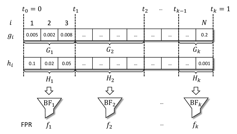
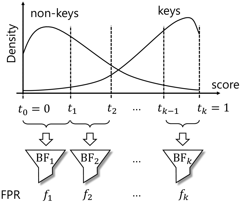
Figure 1: PLBF partitions the score space into k๐‘˜k regions and assigns backup Bloom filters with different FPRs to each region.
Refer to caption
Figure 2: PLBF divides the score space into N๐‘N segments and then clusters the N๐‘N segments into k๐‘˜k regions. PLBF uses dynamic programming to find the optimal way to cluster segments into regions.

First, we define terms to describe PLBF vaidya2021partitioned . Let ๐’ฎ๐’ฎ\mathcal{S} be a set of elements for which the Bloom filter is to be built, and let ๐’ฌ๐’ฌ\mathcal{Q} be the set of elements not included in ๐’ฎ๐’ฎ\mathcal{S} that is used when constructing PLBF (๐’ฎโˆฉ๐’ฌ=โˆ…๐’ฎ๐’ฌ\mathcal{S}\cap\mathcal{Q}=\varnothing). The elements included in ๐’ฎ๐’ฎ\mathcal{S} are called keys, and those not included are called non-keys. To build PLBF, a machine learning model is trained to predict whether a given element x๐‘ฅx is included in the set ๐’ฎ๐’ฎ\mathcal{S} or ๐’ฌ๐’ฌ\mathcal{Q}. For a given element x๐‘ฅx, the machine learning model outputs a score sโ€‹(x)โˆˆ[0,1]๐‘ ๐‘ฅ01s(x)\in[0,1]. The score sโ€‹(x)๐‘ ๐‘ฅs(x) indicates โ€œhow likely is x๐‘ฅx to be included in the set ๐’ฎ๐’ฎ\mathcal{S}.โ€

Next, we explain the design of PLBF. PLBF partitions the score space [0,1]01[0,1] into k๐‘˜k regions and assigns backup Bloom filters with different FPRs to each region (Figureย 2). Given a target overall FPR, Fโˆˆ(0,1)๐น01F\in(0,1), we optimize ๐’•โˆˆโ„k+1๐’•superscriptโ„๐‘˜1\bm{t}\in\mathbb{R}^{k+1} and ๐’‡โˆˆโ„k๐’‡superscriptโ„๐‘˜\bm{f}\in\mathbb{R}^{k} to minimize the total memory usage. Here, ๐’•๐’•\bm{t} is a vector of thresholds for partitioning the score space into k๐‘˜k regions, and ๐’‡๐’‡\bm{f} is a vector of FPRs for each region, satisfying t0=0<t1<โ‹ฏ<tk=1subscript๐‘ก00subscript๐‘ก1โ‹ฏsubscript๐‘ก๐‘˜1t_{0}=0<t_{1}<\dots<t_{k}=1 and 0<fiโ‰ค1โ€‹(i=1โ€‹โ€ฆโ€‹k)0subscript๐‘“๐‘–1๐‘–1โ€ฆ๐‘˜0<f_{i}\leq 1~{}(i=1\dots k).

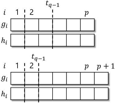
Next, we explain how PLBF finds the optimal ๐’•๐’•\bm{t} and ๐’‡๐’‡\bm{f}. PLBF divides the score space [0,1]01[0,1] into N(>k)annotated๐‘absent๐‘˜N(>k) segments and then finds the optimal ๐’•๐’•\bm{t} and ๐’‡๐’‡\bm{f} using DP. Deciding how to cluster N๐‘N segments into k๐‘˜k consecutive regions corresponds to determining the threshold ๐’•๐’•\bm{t} (Figureย 2). We denote the probabilities that the key and non-key scores are contained in the i๐‘–i-th segment by gisubscript๐‘”๐‘–g_{i} and hisubscriptโ„Ž๐‘–h_{i}, respectively. After we cluster the segments (i.e., determine the thresholds ๐’•๐’•\bm{t}), we denote the probabilities that the key and non-key scores are contained in the i๐‘–i-th region by Gisubscript๐บ๐‘–G_{i} and Hisubscript๐ป๐‘–H_{i}, respectively (e.g., g1+g2+g3=G1subscript๐‘”1subscript๐‘”2subscript๐‘”3subscript๐บ1g_{1}+g_{2}+g_{3}=G_{1} in Figureย 2).

We can find the thresholds ๐’•๐’•\bm{t} that minimize memory usage by solving the following problem for each j=kโ€‹โ€ฆโ€‹N๐‘—๐‘˜โ€ฆ๐‘j=k\dots N (see the appendix for details); we find a way to cluster the 111st to (jโˆ’1)๐‘—1(j-1)-th segments into kโˆ’1๐‘˜1k-1 regions while maximizing

โˆ‘i=1kโˆ’1Giโ€‹log2โก(GiHi).superscriptsubscript๐‘–1๐‘˜1subscript๐บ๐‘–subscript2subscript๐บ๐‘–subscript๐ป๐‘–\sum_{i=1}^{k-1}G_{i}\log_{2}\left(\frac{G_{i}}{H_{i}}\right). (1)

PLBF solves this problem by building a jร—k๐‘—๐‘˜j\times k DP table DPKLjโ€‹[p]โ€‹[q]superscriptsubscriptDPKL๐‘—delimited-[]๐‘delimited-[]๐‘ž\mathrm{DP}_{\mathrm{KL}}^{j}[p][q] (p=0โ€‹โ€ฆโ€‹jโˆ’1๐‘0โ€ฆ๐‘—1p=0\dots j-1 and q=0โ€‹โ€ฆโ€‹kโˆ’1๐‘ž0โ€ฆ๐‘˜1q=0\dots k-1) for each j๐‘—j. DPKLjโ€‹[p]โ€‹[q]superscriptsubscriptDPKL๐‘—delimited-[]๐‘delimited-[]๐‘ž\mathrm{DP}_{\mathrm{KL}}^{j}[p][q] denotes the maximum value of โˆ‘i=1qGiโ€‹log2โก(GiHi)superscriptsubscript๐‘–1๐‘žsubscript๐บ๐‘–subscript2subscript๐บ๐‘–subscript๐ป๐‘–\sum_{i=1}^{q}{G_{i}}\log_{2}\left(\frac{G_{i}}{H_{i}}\right) one can get when you cluster the 111st to p๐‘p-th segments into q๐‘žq regions. To construct PLBF, one must find a clustering method that achieves DPKLjโ€‹[jโˆ’1]โ€‹[kโˆ’1]superscriptsubscriptDPKL๐‘—delimited-[]๐‘—1delimited-[]๐‘˜1\mathrm{DP}_{\mathrm{KL}}^{j}[j-1][k-1]. DPKLjsuperscriptsubscriptDPKL๐‘—\mathrm{DP}_{\mathrm{KL}}^{j} can be computed recursively as follows:

DPKLjโ€‹[p]โ€‹[q]={0(p=0โˆงq=0)โˆ’โˆž((p=0โˆงq>0)โˆจ(p>0โˆงq=0))maxi=1โ€‹โ€ฆโ€‹pโก(DPKLjโ€‹[iโˆ’1]โ€‹[qโˆ’1]+dKLโ€‹(i,p))(else),superscriptsubscriptDPKL๐‘—delimited-[]๐‘delimited-[]๐‘žcases0๐‘0๐‘ž0๐‘0๐‘ž0๐‘0๐‘ž0subscript๐‘–1โ€ฆ๐‘superscriptsubscriptDPKL๐‘—delimited-[]๐‘–1delimited-[]๐‘ž1subscript๐‘‘KL๐‘–๐‘else\mathrm{DP}_{\mathrm{KL}}^{j}[p][q]=\begin{dcases}0&(p=0\land q=0)\\ -\infty&((p=0\land q>0)\lor(p>0\land q=0))\\ \max_{i=1\dots p}\left(\mathrm{DP}_{\mathrm{KL}}^{j}[i-1][q-1]+d_{\mathrm{KL}}(i,p)\right)&(\rm{else}),\end{dcases} (2)

where the function dKLโ€‹(il,ir)subscript๐‘‘KLsubscript๐‘–๐‘™subscript๐‘–๐‘Ÿd_{\mathrm{KL}}(i_{l},i_{r}) is the following function defined for integers ilsubscript๐‘–๐‘™i_{l} and irsubscript๐‘–๐‘Ÿi_{r} satisfying 1โ‰คilโ‰คirโ‰คN1subscript๐‘–๐‘™subscript๐‘–๐‘Ÿ๐‘1\leq i_{l}\leq i_{r}\leq N:

dKLโ€‹(il,ir)=(โˆ‘i=ilirgi)โ€‹log2โก(โˆ‘i=ilirgiโˆ‘i=ilirhi).subscript๐‘‘KLsubscript๐‘–๐‘™subscript๐‘–๐‘Ÿsuperscriptsubscript๐‘–subscript๐‘–๐‘™subscript๐‘–๐‘Ÿsubscript๐‘”๐‘–subscript2superscriptsubscript๐‘–subscript๐‘–๐‘™subscript๐‘–๐‘Ÿsubscript๐‘”๐‘–superscriptsubscript๐‘–subscript๐‘–๐‘™subscript๐‘–๐‘Ÿsubscriptโ„Ž๐‘–d_{\mathrm{KL}}(i_{l},i_{r})=\left(\sum_{i=i_{l}}^{i_{r}}g_{i}\right)\log_{2}\left(\frac{\sum_{i=i_{l}}^{i_{r}}g_{i}}{\sum_{i=i_{l}}^{i_{r}}h_{i}}\right). (3)

The time complexity to construct this DP table is ๐’ชโ€‹(j2โ€‹k)๐’ชsuperscript๐‘—2๐‘˜\mathcal{O}(j^{2}k). Then, by tracing the recorded transitions backward from DPKLjโ€‹[jโˆ’1]โ€‹[kโˆ’1]superscriptsubscriptDPKL๐‘—delimited-[]๐‘—1delimited-[]๐‘˜1\mathrm{DP}_{\mathrm{KL}}^{j}[j-1][k-1], we obtain the best clustering with a time complexity of ๐’ชโ€‹(k)๐’ช๐‘˜\mathcal{O}(k). As the DP table is constructed for each j=kโ€‹โ€ฆโ€‹N๐‘—๐‘˜โ€ฆ๐‘j=k\dots N, the overall complexity is ๐’ชโ€‹(N3โ€‹k)๐’ชsuperscript๐‘3๐‘˜\mathcal{O}(N^{3}k). The pseudo-code for PLBF construction is provided in the appendix.

We can divide the score space more finely with a larger N๐‘N and thus obtain a near-optimal ๐’•๐’•\bm{t}. However, the time complexity increases rapidly with increasing N๐‘N.

3 Fast PLBF

We propose fast PLBF, which constructs the same data structure as PLBF more quickly than PLBF by omitting the redundant construction of DP tables. Fast PLBF uses the same design as PLBF and finds the best clustering (i.e., ๐’•๐’•\bm{t}) and FPRs (i.e., ๐’‡๐’‡\bm{f}) to minimize memory usage.

PLBF constructs a DP table for each j=kโ€‹โ€ฆโ€‹N๐‘—๐‘˜โ€ฆ๐‘j=k\dots N. We found that this computation is redundant and that we can also use the last DP table DPKLNsuperscriptsubscriptDPKL๐‘\mathrm{DP}_{\mathrm{KL}}^{N} for j=kโ€‹โ€ฆโ€‹Nโˆ’1๐‘—๐‘˜โ€ฆ๐‘1j=k\dots N-1. This is because the maximum value of โˆ‘i=1kโˆ’1Giโ€‹log2โก(GiHi)superscriptsubscript๐‘–1๐‘˜1subscript๐บ๐‘–subscript2subscript๐บ๐‘–subscript๐ป๐‘–\sum_{i=1}^{k-1}G_{i}\log_{2}\left(\frac{G_{i}}{H_{i}}\right) when clustering the 111st to (jโˆ’1)๐‘—1(j-1)-th segments into kโˆ’1๐‘˜1k-1 regions is equal to DPKLNโ€‹[jโˆ’1]โ€‹[kโˆ’1]superscriptsubscriptDPKL๐‘delimited-[]๐‘—1delimited-[]๐‘˜1\mathrm{DP}_{\mathrm{KL}}^{N}[j-1][k-1]. We can obtain the best clustering by tracing the transitions backward from DPKLNโ€‹[jโˆ’1]โ€‹[kโˆ’1]superscriptsubscriptDPKL๐‘delimited-[]๐‘—1delimited-[]๐‘˜1\mathrm{DP}_{\mathrm{KL}}^{N}[j-1][k-1]. The time complexity of tracing the transitions is ๐’ชโ€‹(k)๐’ช๐‘˜\mathcal{O}(k), which is faster than constructing the DP table.

This is a simple method, but it is a method that only becomes apparent after some organization on the optimization problem of PLBF. PLBF solves Nโˆ’k+1๐‘๐‘˜1N-k+1 optimization problems separately, i.e., for each of j=k,โ€ฆ,N๐‘—๐‘˜โ€ฆ๐‘j=k,\dots,N, the problem of โ€œfinding the optimal ๐’•๐’•\bm{t} and ๐’‡๐’‡\bm{f} when the k๐‘˜k-th region consists of the j,โ€ฆ,N๐‘—โ€ฆ๐‘j,\dots,Nth segmentsโ€ is solved separately. Fast PLBF, on the other hand, solves the problems for j=k,โ€ฆ,Nโˆ’1๐‘—๐‘˜โ€ฆ๐‘1j=k,\dots,N-1 faster by reusing the computations in the problem for j=N๐‘—๐‘j=N. The reorganization of the problem in the appendix makes it clear that this reuse does not change the answer.

The pseudo-code for fast PLBF construction is provided in the appendix. The time complexity of building DPKLNsuperscriptsubscriptDPKL๐‘\mathrm{DP}_{\mathrm{KL}}^{N} is ๐’ชโ€‹(N2โ€‹k)๐’ชsuperscript๐‘2๐‘˜\mathcal{O}(N^{2}k), and the worst-case complexity of subsequent computations is ๐’ชโ€‹(Nโ€‹k2)๐’ช๐‘superscript๐‘˜2\mathcal{O}(Nk^{2}). Because N>k๐‘๐‘˜N>k, the total complexity is ๐’ชโ€‹(N2โ€‹k)๐’ชsuperscript๐‘2๐‘˜\mathcal{O}(N^{2}k), which is faster than ๐’ชโ€‹(N3โ€‹k)๐’ชsuperscript๐‘3๐‘˜\mathcal{O}(N^{3}k) for PLBF, although fast PLBF constructs the same data structure as PLBF.

Fast PLBF extends the usability of PLBF. In any application of PLBF, fast PLBF can be used instead of PLBF because fast PLBF can be constructed quickly without losing the accuracy of PLBF. Fast PLBF has applications in a wide range of computing areas feng2011efficient ; chang2008bigtable , and is significantly superior in applications where construction is frequently performed. Fast PLBF also has the advantage of simplifying hyperparameter settings. When using PLBF, the hyperparameters N๐‘N and k๐‘˜k must be carefully determined, considering the trade-off between accuracy and construction speed. With fast PLBF, on the other hand, it is easy to determine the appropriate hyperparameters because the construction time is short enough, even if N๐‘N and k๐‘˜k are set somewhat large.

4 Fast PLBF++

Refer to caption
Refer to caption
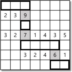
Figure 3: The cases 3 where there is no โ€œcrossingโ€ of the recorded transitions when computing DPKLโ€‹[p]โ€‹[q]โ€‹(p=1โ€‹โ€ฆโ€‹Nโˆ’1)subscriptDPKLdelimited-[]๐‘delimited-[]๐‘ž๐‘1โ€ฆ๐‘1\mathrm{DP}_{\mathrm{KL}}[p][q]~{}(p=1\dots N-1) from DPKLโ€‹[p]โ€‹[qโˆ’1]โ€‹(p=0โ€‹โ€ฆโ€‹Nโˆ’2)subscriptDPKLdelimited-[]๐‘delimited-[]๐‘ž1๐‘0โ€ฆ๐‘2\mathrm{DP}_{\mathrm{KL}}[p][q-1]~{}(p=0\dots N-2) and 3 where there is. The arrows indicate which transition took the maximum value. Empirically, the probability of โ€œcrossingโ€ is small.
Refer to caption
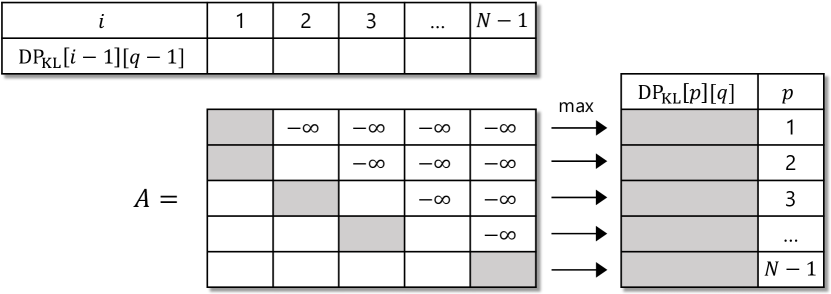
Figure 4: Computing DPKLโ€‹[p]โ€‹[q]โ€‹(p=1โ€‹โ€ฆโ€‹Nโˆ’1)subscriptDPKLdelimited-[]๐‘delimited-[]๐‘ž๐‘1โ€ฆ๐‘1\mathrm{DP}_{\mathrm{KL}}[p][q]~{}(p=1\dots N-1) from DPKLโ€‹[p]โ€‹[qโˆ’1]โ€‹(p=0โ€‹โ€ฆโ€‹Nโˆ’2)subscriptDPKLdelimited-[]๐‘delimited-[]๐‘ž1๐‘0โ€ฆ๐‘2\mathrm{DP}_{\mathrm{KL}}[p][q-1]~{}(p=0\dots N-2) via the matrix A๐ดA. The computation is the same as solving the matrix problem for matrix A๐ดA. When the score distribution is ideal, A๐ดA is a monotone matrix.
Refer to caption
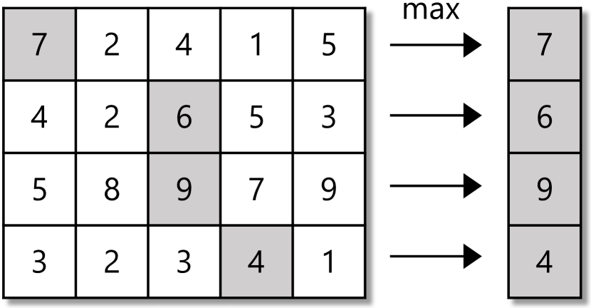
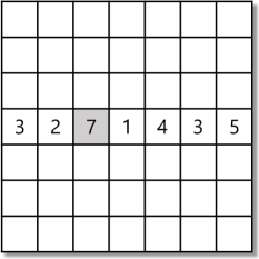
Figure 5: Example of a matrix problem for a 4ร—5454\times 5 monotone matrix. The position of the maximum value in each row (filled in gray) is moved to the โ€œlower rightโ€.

We propose fast PLBF++, which can be constructed even faster than fast PLBF. Fast PLBF++ accelerates the construction of the DP table DPKLNsuperscriptsubscriptDPKL๐‘\mathrm{DP}_{\mathrm{KL}}^{N} by taking advantage of a characteristic that DP tables often have. When the transitions recorded in computing DPKLNโ€‹[p]โ€‹[q]โ€‹(p=1โ€‹โ€ฆโ€‹Nโˆ’1)superscriptsubscriptDPKL๐‘delimited-[]๐‘delimited-[]๐‘ž๐‘1โ€ฆ๐‘1\mathrm{DP}_{\mathrm{KL}}^{N}[p][q]~{}(p=1\dots N-1) from DPKLNโ€‹[p]โ€‹[qโˆ’1]โ€‹(p=0โ€‹โ€ฆโ€‹Nโˆ’2)superscriptsubscriptDPKL๐‘delimited-[]๐‘delimited-[]๐‘ž1๐‘0โ€ฆ๐‘2\mathrm{DP}_{\mathrm{KL}}^{N}[p][q-1]~{}(p=0\dots N-2) are represented by arrows, as in Figureย 3, we find that the arrows rarely โ€œcrossโ€ (at locations other than endpoints). In other words, the transitions tend to have few intersections (Figureย 3) rather than many (Figureย 3). Fast PLBF++ takes advantage of this characteristic to construct the DP table with less complexity ๐’ชโ€‹(Nโ€‹kโ€‹logโกN)๐’ช๐‘๐‘˜๐‘\mathcal{O}(Nk\log N), thereby reducing the total construction complexity to ๐’ชโ€‹(Nโ€‹kโ€‹logโกN+Nโ€‹k2)๐’ช๐‘๐‘˜๐‘๐‘superscript๐‘˜2\mathcal{O}(Nk\log N+Nk^{2}).

First, we define the terms to describe fast PLBF++. For simplicity, DPKLNsuperscriptsubscriptDPKL๐‘\mathrm{DP}_{\mathrm{KL}}^{N} is denoted as DPKLsubscriptDPKL\mathrm{DP}_{\mathrm{KL}} in this section. The (Nโˆ’1)ร—(Nโˆ’1)๐‘1๐‘1(N-1)\times(N-1) matrix A๐ดA is defined as follows:

Apโ€‹i={โˆ’โˆž(i=p+1,p+2,โ€ฆ,Nโˆ’1)DPKLโ€‹[iโˆ’1]โ€‹[qโˆ’1]+dKLโ€‹(i,p)(else).subscript๐ด๐‘๐‘–cases๐‘–๐‘1๐‘2โ€ฆ๐‘1subscriptDPKLdelimited-[]๐‘–1delimited-[]๐‘ž1subscript๐‘‘KL๐‘–๐‘elseA_{pi}=\begin{dcases}-\infty&(i=p+1,p+2,\dots,N-1)\\ \mathrm{DP}_{\mathrm{KL}}[i-1][q-1]+d_{\mathrm{KL}}(i,p)&(\rm{else}).\end{dcases} (4)

Then, from the definition of DPKLsubscriptDPKL\mathrm{DP}_{\mathrm{KL}},

DPKLโ€‹[p]โ€‹[q]=maxi=1โ€‹โ€ฆโ€‹Nโˆ’1โกApโ€‹i.subscriptDPKLdelimited-[]๐‘delimited-[]๐‘žsubscript๐‘–1โ€ฆ๐‘1subscript๐ด๐‘๐‘–\mathrm{DP}_{\mathrm{KL}}[p][q]=\max_{i=1\dots N-1}A_{pi}. (5)

The matrix A๐ดA represents the intermediate calculations involved in determining DPKLโ€‹[p]โ€‹[q]subscriptDPKLdelimited-[]๐‘delimited-[]๐‘ž\mathrm{DP}_{\mathrm{KL}}[p][q] from DPKLโ€‹[p]โ€‹[qโˆ’1]subscriptDPKLdelimited-[]๐‘delimited-[]๐‘ž1\mathrm{DP}_{\mathrm{KL}}[p][q-1] (Figureย 5).

Following Aggarwal et al. aggarwal1987geometric , we define the monotone matrix and matrix problem as follows.

Definition 4.1.

Let B๐ตB be an nร—m๐‘›๐‘šn\times m real matrix, and we define a function J:{1โ€‹โ€ฆโ€‹n}โ†’{1โ€‹โ€ฆโ€‹m}:๐ฝโ†’1โ€ฆ๐‘›1โ€ฆ๐‘šJ:\{1\dots n\}\rightarrow\{1\dots m\}, where Jโ€‹(i)๐ฝ๐‘–J(i) is the jโˆˆ{1โ€‹โ€ฆโ€‹m}๐‘—1โ€ฆ๐‘šj\in\{1\dots m\} such that Biโ€‹jsubscript๐ต๐‘–๐‘—B_{ij} is the maximum value of the i๐‘–i-th row of B๐ตB. If there is more than one such j๐‘—j, let Jโ€‹(i)๐ฝ๐‘–J(i) be the smallest. A matrix B๐ตB is called a monotone matrix if Jโ€‹(i1)โ‰คJโ€‹(i2)๐ฝsubscript๐‘–1๐ฝsubscript๐‘–2J(i_{1})\leq J(i_{2}) for any i1subscript๐‘–1i_{1} and i2subscript๐‘–2i_{2} that satisfy 1โ‰คi1<i2โ‰คn1subscript๐‘–1subscript๐‘–2๐‘›1\leq i_{1}<i_{2}\leq n. Finding the maximum value of each row of a matrix is called a matrix problem.

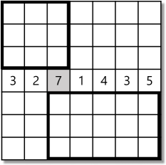
An example of a matrix problem for a monotone matrix is shown in Figureย 5. Solving the matrix problem for a general nร—m๐‘›๐‘šn\times m matrix requires ๐’ชโ€‹(nโ€‹m)๐’ช๐‘›๐‘š\mathcal{O}(nm) time complexity because all matrix values must be checked. Meanwhile, if the matrix is known to be a monotone matrix, the matrix problem for this matrix can be solved with a time complexity of ๐’ชโ€‹(n+mโ€‹logโกn)๐’ช๐‘›๐‘š๐‘›\mathcal{O}(n+m\log n) using the divide-and-conquer algorithm aggarwal1987geometric . Here, the exhaustive search for the middle row and the refinement of the search range are repeated recursively (Figureย 7).

Refer to caption
Refer to caption
Refer to caption
Figure 6: A divide-and-conquer algorithm for solving a matrix problem for a monotone matrix: 7 An exhaustive search is performed on the middle row, and 7 the result is used to narrow down the search area. 7 This is repeated recursively.
Refer to caption
Refer to caption
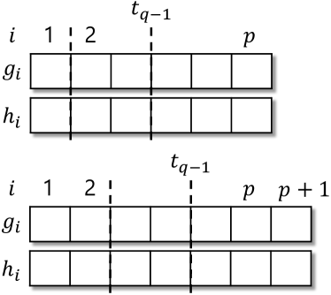
Figure 7: When the number of regions is fixed at q๐‘žq and the number of segments is increased by 111, the optimal tqโˆ’1subscript๐‘ก๐‘ž1t_{q-1} remains unchanged or increases if A๐ดA is a monotone matrix 7. When A๐ดA is not a monotone matrix 7, the optimal tqโˆ’1subscript๐‘ก๐‘ž1t_{q-1} may decrease.

We also define an ideal score distribution as follows.

Definition 4.2.

A score distribution is ideal if the following holds:

g1h1โ‰คg2h2โ‰คโ‹ฏโ‰คgNhN.subscript๐‘”1subscriptโ„Ž1subscript๐‘”2subscriptโ„Ž2โ‹ฏsubscript๐‘”๐‘subscriptโ„Ž๐‘\frac{g_{1}}{h_{1}}\leq\frac{g_{2}}{h_{2}}\leq\dots\leq\frac{g_{N}}{h_{N}}. (6)

An ideal score distribution implies that the probability of xโˆˆ๐’ฎ๐‘ฅ๐’ฎx\in\mathcal{S} and the score sโ€‹(x)๐‘ ๐‘ฅs(x) are ideally well correlated. In other words, an ideal score distribution means that the machine learning model learns the distribution ideally.

โ€œFew crossing transitionsโ€ in Figureย 3 indicates that A๐ดA is a monotone matrix or is close to it. It is somewhat intuitive that A๐ดA is a monotone matrix or is close to it. This is because the fact that A๐ดA is a monotone matrix implies that the optimal tqโˆ’1subscript๐‘ก๐‘ž1t_{q-1} does not decrease when the number of regions is fixed at q๐‘žq and the number of segments increases by 111 (Figureย 7). It is intuitively more likely that tqโˆ’1subscript๐‘ก๐‘ž1t_{q-1} remains unchanged or increases, as in Figureย 7, than that tqโˆ’1subscript๐‘ก๐‘ž1t_{q-1} decreases, as in Figureย 7. Fast PLBF++ takes advantage of this insight to rapidly construct DP tables.

From Equation (5), determining DPKLโ€‹[p]โ€‹[q]โ€‹(p=1โ€‹โ€ฆโ€‹Nโˆ’1)subscriptDPKLdelimited-[]๐‘delimited-[]๐‘ž๐‘1โ€ฆ๐‘1\mathrm{DP}_{\mathrm{KL}}[p][q]~{}(p=1\dots N-1) from DPKLโ€‹[p]โ€‹[qโˆ’1]โ€‹(p=0โ€‹โ€ฆโ€‹Nโˆ’2)subscriptDPKLdelimited-[]๐‘delimited-[]๐‘ž1๐‘0โ€ฆ๐‘2\mathrm{DP}_{\mathrm{KL}}[p][q-1]~{}(p=0\dots N-2) is equivalent to solving the matrix problem of matrix A๐ดA. When A๐ดA is a monotone matrix, the divide-and-conquer algorithm can solve this problem with ๐’ชโ€‹(Nโ€‹logโกN)๐’ช๐‘๐‘\mathcal{O}(N\log N) time complexity. (The same algorithm can obtain a not necessarily correct solution even if A๐ดA is not a monotone matrix.) By computing DPKLโ€‹[p]โ€‹[q]subscriptDPKLdelimited-[]๐‘delimited-[]๐‘ž\mathrm{DP}_{\mathrm{KL}}[p][q] with this algorithm sequentially for q=1โ€‹โ€ฆโ€‹kโˆ’1๐‘ž1โ€ฆ๐‘˜1q=1\dots k-1, we can construct a DP table with a time complexity of ๐’ชโ€‹(Nโ€‹kโ€‹logโกN)๐’ช๐‘๐‘˜๐‘\mathcal{O}(Nk\log N). The worst-case complexity of the subsequent calculations is ๐’ชโ€‹(Nโ€‹k2)๐’ช๐‘superscript๐‘˜2\mathcal{O}(Nk^{2}), so the total complexity is ๐’ชโ€‹(Nโ€‹kโ€‹logโกN+Nโ€‹k2)๐’ช๐‘๐‘˜๐‘๐‘superscript๐‘˜2\mathcal{O}(Nk\log N+Nk^{2}). This is the fast PLBF++ construction algorithm, and this is faster than fast PLBF, which requires ๐’ชโ€‹(N2โ€‹k)๐’ชsuperscript๐‘2๐‘˜\mathcal{O}(N^{2}k) computations.

Fast PLBF++ does not necessarily have the same data structure as PLBF because A๐ดA is not necessarily a monotone matrix. However, as the following theorem shows, we can prove that A๐ดA is a monotone matrix under certain conditions.

Theorem 4.3.

If the score distribution is ideal, A๐ดA is a monotone matrix.

The proof is given in the appendix. When the distribution is not ideal, matrix A๐ดA is not necessarily a monotone matrix, but as mentioned above, it is somewhat intuitive that A๐ดA is close to a monotone matrix. In addition, as will be shown in the next section, experiment results from real-world datasets whose distribution is not ideal show that fast PLBF++ is almost as memory efficient as PLBF.

5 Experiments
Refer to caption
(a) Malicious URLs Dataset
Refer to caption
(b) EMBER Dataset
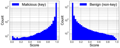
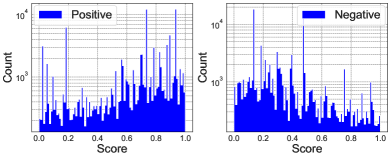
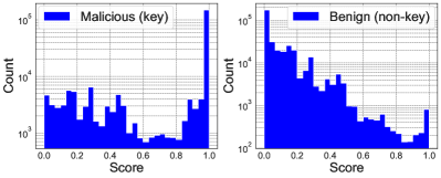
Figure 8: Histograms of the score distributions of keys and non-keys.
Refer to caption
(a) Malicious URLs Dataset
Refer to caption
(b) EMBER Dataset
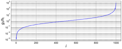
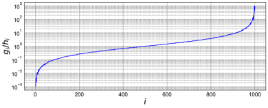
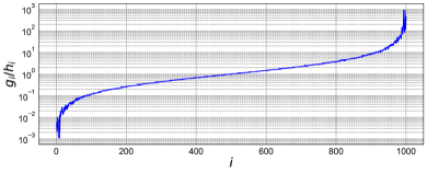
Figure 9: Ratio of keys to non-keys.

This section evaluates the experimental performance of fast PLBF and fast PLBF++. We compared the performances of fast PLBF and fast PLBF++ with four baselines: Bloom filter bloom1970space , Ada-BF dai2020adaptive , sandwiched learned Bloom filter (sandwiched LBF) mitzenmacher2018model , and PLBF vaidya2021partitioned . Similar to PLBF, Ada-BF is an LBF that partitions the score space into several regions and assigns different FPRs to each region. However, Ada-BF relies heavily on heuristics for clustering and assigning FPRs. Sandwiched LBF is an LBF that โ€œsandwichesโ€ a machine learning model with two Bloom filters. This achieves better memory efficiency than the original LBF by optimizing the size of two Bloom filters.

To facilitate the comparison of different methods or hyperparameters results, we have slightly modified the original PLBF framework. The original PLBF was designed to minimize memory usage under the condition of a given false positive rate. However, this approach makes it difficult to compare the results of different methods or hyperparameters. This is because both the false positive rate at test time and the memory usage vary depending on the method and hyperparameters, which often makes it difficult to determine the superiority of the results. Therefore, in our experiments, we used a framework where the expected false positive rate is minimized under the condition of memory usage. This approach makes it easy to obtain two results with the same memory usage and compare them by the false positive rate at test time. See the appendix for more information on how this framework modification will change the construction method of PLBFs.

Datasets: We evaluated the algorithms using the following two datasets.

  • โ€ข

    Malicious URLs Dataset: As in previous papers dai2020adaptive ; vaidya2021partitioned , we used Malicious URLs Dataset manu2021urlDataset . The URLs dataset comprises 223,088 malicious and 428,118 benign URLs. We extracted 20 lexical features such as URL length, use of shortening, number of special characters, etc. We used all malicious URLs and 342,482 (80%) benign URLs as the training set, and the remaining benign URLs as the test set.

  • โ€ข

    EMBER Dataset: We used the EMBER dataset anderson2018ember as in the PLBF research. The dataset consists of 300,000 malicious and 400,000 benign files, along with the features of each file. We used all malicious files and 300,000 (75%) benign files as the train set and the remaining benign files as the test set.

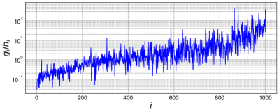
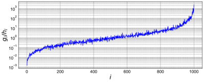
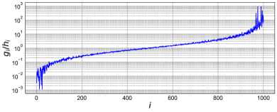
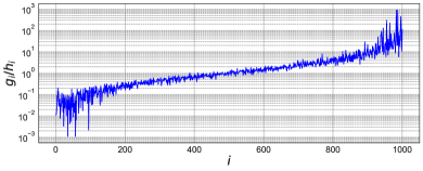
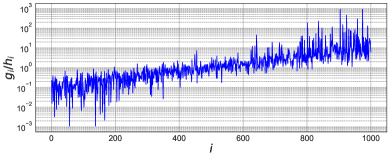
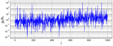
While any model can be used for the classifier, we used LightGBM NIPS2017_6449f44a because of its speed in training and inference, as well as its memory efficiency and accuracy. The sizes of the machine learning model for the URLs and EMBER datasets are 312 Kb and 1.19 Mb, respectively. The training time of the machine learning model for the URLs and EMBER datasets is 1.09 and 2.71 seconds, respectively. The memory usage of LBF is the total memory usage of the backup Bloom filters and the machine learning model. Figureย 8 shows a histogram of each datasetโ€™s score distributions of keys and non-keys. We can see that the frequency of keys increases and that of non-keys decreases as the score increases. In addition, Figureย 9 plots gi/hiโ€‹(i=1โ€‹โ€ฆโ€‹N)subscript๐‘”๐‘–subscriptโ„Ž๐‘–๐‘–1โ€ฆ๐‘g_{i}/h_{i}~{}(i=1\dots N) when N=1,000๐‘1000N=1,000. We can see that gi/hisubscript๐‘”๐‘–subscriptโ„Ž๐‘–g_{i}/h_{i} tends to increase as i๐‘–i increases, but the increase is not monotonic (i.e., the score distribution is not ideal).

5.1 Construction time

Refer to caption
Refer to caption
(a) Malicious URLs Dataset
Refer to caption
(b) EMBER Dataset
Figure 10: Construction time.

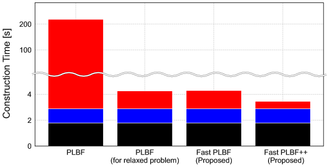
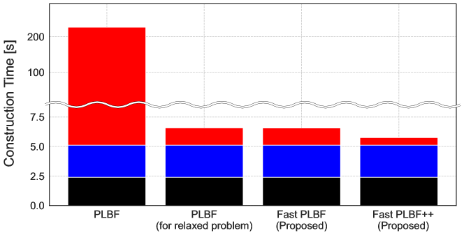
We compared the construction times of fast PLBF and fast PLBF++ with those of existing methods. Following the experiments in the PLBF paper, hyperparameters for PLBF, fast PLBF, and fast PLBF++ were set to N=1,000๐‘1000N=1,000 and k=5๐‘˜5k=5.

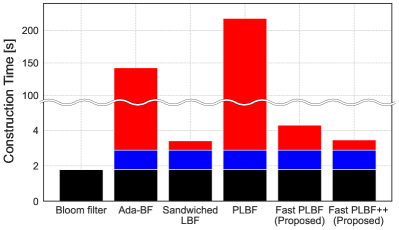
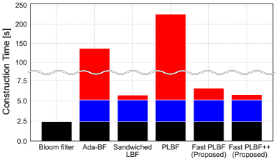
Figureย 10 shows the construction time for each method. The construction time for learned Bloom filters includes not only the time to insert keys into the Bloom filters but also the time to train the machine learning model and the time to compute the optimal parameters (๐’•๐’•\bm{t} and ๐’‡๐’‡\bm{f} in the case of PLBF).

Ada-BF and sandwiched LBF use heuristics to find the optimal parameters, so they have shorter construction times than PLBF but have worse accuracy. PLBF has better accuracy but takes more than 3 minutes to find the optimal ๐’•๐’•\bm{t} and ๐’‡๐’‡\bm{f}. On the other hand, our fast PLBF and fast PLBF++ take less than 2 seconds. As a result, Fast PLBF constructs 50.8 and 34.3 times faster than PLBF, and fast PLBF++ constructs 63.1 and 39.3 times faster than PLBF for the URLs and EMBER datasets, respectively. This is about the same construction time as sandwiched LBF, which relies heavily on heuristics and, as we will see in the next section, is much less accurate than PLBF.

5.2 Memory Usage and FPR

Refer to caption
Refer to caption
(a) Malicious URLs Dataset
Refer to caption
(b) EMBER Dataset
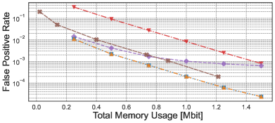
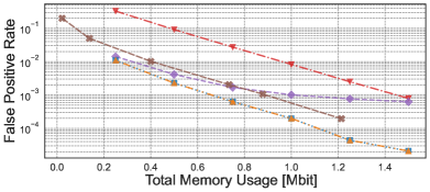
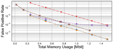
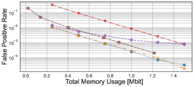
Figure 11: Trade-off between memory usage and FPR.

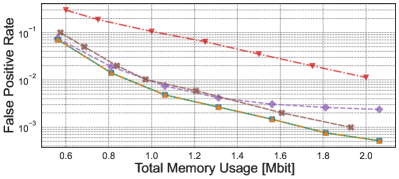
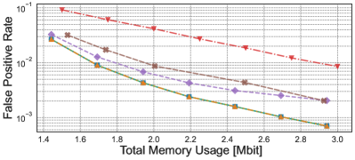
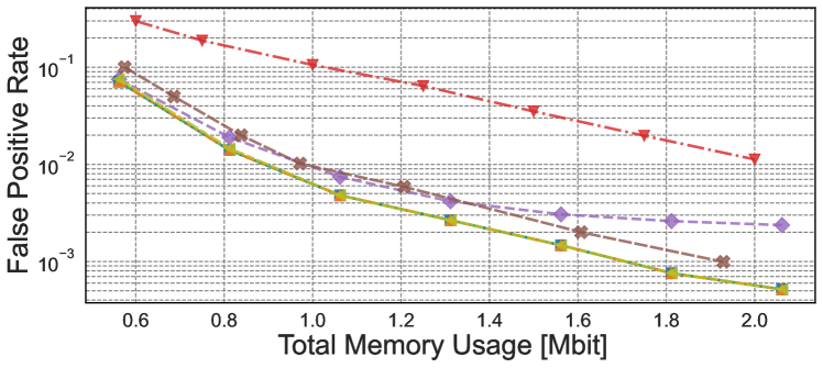
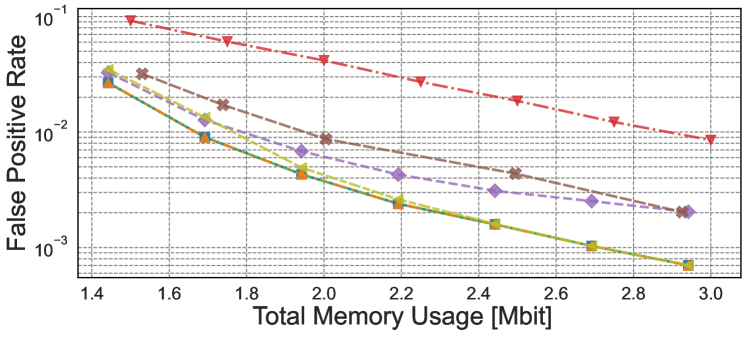
We compared the trade-off between memory usage and FPR for fast PLBF and fast PLBF++ with Bloom filter, Ada-BF, sandwiched LBF, and PLBF. Following the experiments in the PLBF paper, hyperparameters for PLBF, fast PLBF, and fast PLBF++ were always set to N=1,000๐‘1000N=1,000 and k=5๐‘˜5k=5.

Figureย 11 shows each methodโ€™s trade-off between memory usage and FPR. PLBF, fast PLBF, and fast PLBF++ have better Pareto curves than the other methods for all datasets. Fast PLBF constructs the same data structure as PLBF in all cases, so it has exactly the same accuracy as PLBF. Fast PLBF++ achieves almost the same accuracy as PLBF. Fast PLBF++ has up to 1.0019 and 1.000083 times higher false positive rates than PLBF for the URLs and EMBER datasets, respectively.

5.3 Ablation study for hyper-parameters

Refer to caption
Refer to caption
(a) Malicious URLs Dataset
Refer to caption
(b) EMBER Dataset
Figure 12: Ablation study for hyper-parameter N๐‘N.
Refer to caption
Refer to caption
(a) Malicious URLs Dataset
Refer to caption
(b) EMBER Dataset
Figure 13: Ablation study for hyper-parameter k๐‘˜k.

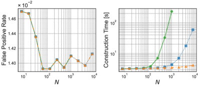
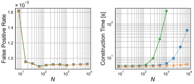
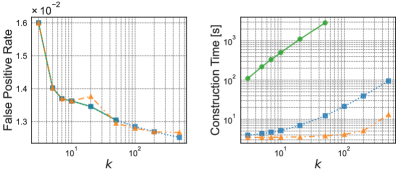
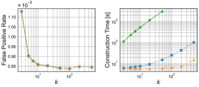
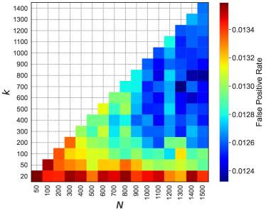
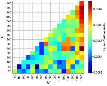
The parameters of the PLBFs are memory size, N๐‘N, and k๐‘˜k. The memory size is specified by the user, and N๐‘N and k๐‘˜k are hyperparameters that are determined by balancing construction time and accuracy. In the previous sections, we set N๐‘N to 1,000 and k๐‘˜k to 5, following the original paper on PLBF. In this section, we perform ablation studies for these hyperparameters to confirm that our proposed methods can construct accurate data structures quickly, no matter what hyperparameter settings are used. We also confirm that the accuracy tends to be better and the construction time increases as N๐‘N and k๐‘˜k are increased, and that the construction time of the proposed methods increases much slower than PLBF.

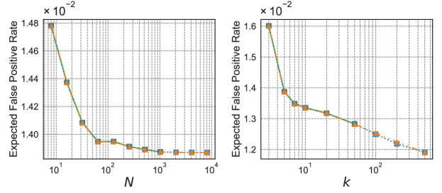
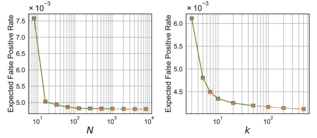
Figureย 12 shows the construction time and false positive rate with various N๐‘N while the memory usage of the backup Bloom filters is fixed at 500 Kb and k๐‘˜k is fixed at 5. For all three PLBFs, the false positive rate tends to decrease as N๐‘N increases. (Note that this is the false positive rate on test data, so it does not necessarily decrease monotonically. The appendix shows that the expected value of the false positive rate calculated using training data decreases monotonically as N๐‘N increases.) Also, as N๐‘N increases, the PLBF construction time increases rapidly, but the fast PLBF construction time increases much more slowly than that, and for fast PLBF++, the construction time changes little. This is because the construction time of PLBF is asymptotically proportional to N3superscript๐‘3N^{3}, while that of fast PLBF and fast PLBF++ is proportional to N2superscript๐‘2N^{2} and Nโ€‹logโกN๐‘๐‘N\log N, respectively. The experimental results show that the two proposed methods can achieve high accuracy without significantly changing the construction time with large N๐‘N.

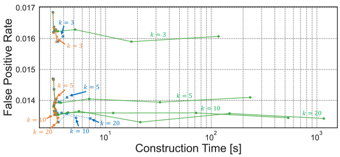
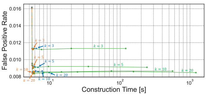
Figureย 13 shows the construction time and false positive rate with various k๐‘˜k while the backup bloom filter memory usage is fixed at 500 Kb and N๐‘N is fixed at 1,000. For all three PLBFs, the false positive rate tends to decrease as k๐‘˜k increases. For the EMBER dataset, the false positive rate stops decreasing at about k=20๐‘˜20k=20, while for the URLs dataset, it continues to decrease even at about k=500๐‘˜500k=500. (Just as in the case of experiments with varying N๐‘N, this decrease is not necessarily monotonic.) In addition, the construction times of all three PLBFs increase proportionally to k๐‘˜k, but fast PLBF has a much shorter construction time than PLBF, and fast PLBF++ has an even shorter construction time than fast PLBF. When k=50๐‘˜50k=50, fast PLBF constructs 233 and 199 times faster than PLBF, and fast PLBF++ constructs 761 and 500 times faster than PLBF for the URLs and EMBER datasets, respectively. The experimental results indicate that by increasing k๐‘˜k, the two proposed methods can achieve high accuracy without significantly affecting the construction time.

6 Related Work

Approximate membership query is a query that asks whether the query q๐‘žq is contained in the set ๐’ฎ๐’ฎ\mathcal{S} while allowing for false positives with a small probability ฮต๐œ€\varepsilon. One can prove that at least |๐’ฎ|โ€‹log2โก(1ฮต)๐’ฎsubscript21๐œ€|\mathcal{S}|\log_{2}\left(\frac{1}{\varepsilon}\right) bits of memory must be used to answer the approximate membership query if the elements in the set or queries are selected with equal probability from the universal set carter1978exact .

A Bloom filter bloom1970space is one of the most basic data structures for approximate membership queries. It compresses the set ๐’ฎ๐’ฎ\mathcal{S} into a bit string using hash functions. This bit string and the hash functions are then used to answer the queries. To achieve an FPR of ฮต๐œ€\varepsilon, a Bloom filter requires |๐’ฎ|โ€‹log2โก(1ฮต)โ€‹log2โกe๐’ฎsubscript21๐œ€subscript2๐‘’|\mathcal{S}|\log_{2}\left(\frac{1}{\varepsilon}\right)\log_{2}e bits of memory. This is log2โกesubscript2๐‘’\log_{2}e times the theoretical lower bound.

Various derivatives have been proposed that achieve better memory efficiency than the original Bloom filter. The cuckoo filter fan2014cuckoo is more memory efficient than the original Bloom filter and supports dynamic addition and removal of elements. Pagh et al. pagh2005optimal proposed a replacement for Bloom filter that achieves a theoretical lower bound. Various other memory-efficient filters exist, including the vacuum filter wang2019vacuum , xor filter graf2020xor , and ribbon filter peter2021ribbon . However, these derivatives do not consider the structure of the distribution and thus cannot take advantage of it.

Kraska et al.kraska2018case proposed using a machine learning model as a prefilter of a backup Bloom filter. Ada-BF dai2020adaptive extended this design and proposed to exploit the scores output by the machine learning model. PLBF vaidya2021partitioned uses a design similar to that of Ada-BF but introduces fewer heuristics for optimization than Ada-BF. Mitzenmacher mitzenmacher2018model proposed an LBF that โ€œsandwichesโ€ a machine learning model with two Bloom filters. This achieves better memory efficiency than the original LBF but can actually be interpreted as a special case of PLBF.

7 Limitation and Future Work

As explained in Sectionย 4, it is somewhat intuitive that A๐ดA is a monotone matrix or close to it, so it is also intuitive that fast PLBF++ achieves accuracy close to PLBF. Experimental results on the URLs and EMBER datasets also suggest that fast PLBF++ achieves almost the same accuracy as PLBF, even when the score distribution is not ideal. This experimental rule is further supported by the results of the artificial data experiments described in the appendix. However, there is no theoretical support for the accuracy of fast PLBF++. Theoretical support for how fast PLBF++ accuracy may degrade relative to PLBF is a future issue.

Besides, it is possible to consider faster methods by making stronger assumptions than fast PLBF++. Fast PLBF++ assumes the monotonicity of matrix A๐ดA. We adopted this assumption because matrix A๐ดA is proved to be monotone under intuitive assumptions about the data distribution. However, by assuming stronger assumptions about matrix A๐ดA, the computational complexity of the construction could be further reduced. For example, if matrix A๐ดA is totally monotone, the matrix problem for matrix A๐ดA can be solved in ๐’ชโ€‹(N)๐’ช๐‘\mathcal{O}(N) using algorithms such as aggarwal1987geometric ; galil1989linear . Using such existing DP algorithms is a promising direction toward even faster or more accurate methods, and is a future work.

8 Conclusion

PLBF is an outstanding LBF that can effectively utilize the distribution of the set and queries captured by a machine learning model. However, PLBF is computationally expensive to construct. We proposed fast PLBF and fast PLBF++ to solve this problem. Fast PLBF is superior to PLBF because fast PLBF constructs exactly the same data structure as PLBF but does so faster. Fast PLBF++ is even faster than fast PLBF and achieves almost the same accuracy as PLBF and fast PLBF. These proposed methods have greatly expanded the range of applications of PLBF.

Acknowledgments and Disclosure of Funding

We thank the anonymous reviewers for their constructive comments. This work was supported by JST AIP Acceleration Research JPMJCR23U2, Japan.

References

  • (1) Burtonย H Bloom. Space/time trade-offs in hash coding with allowable errors. Communications of the ACM, 13(7):422โ€“426, 1970.
  • (2) Andrei Broder and Michael Mitzenmacher. Network applications of bloom filters: A survey. Internet mathematics, 1(4):485โ€“509, 2004.
  • (3) Sasu Tarkoma, Christianย Esteve Rothenberg, and Eemil Lagerspetz. Theory and practice of bloom filters for distributed systems. IEEE Communications Surveys & Tutorials, 14(1):131โ€“155, 2011.
  • (4) Shahabeddin Geravand and Mahmood Ahmadi. Bloom filter applications in network security: A state-of-the-art survey. Computer Networks, 57(18):4047โ€“4064, 2013.
  • (5) Fay Chang, Jeffrey Dean, Sanjay Ghemawat, Wilsonย C Hsieh, Deborahย A Wallach, Mike Burrows, Tushar Chandra, Andrew Fikes, and Robertย E Gruber. Bigtable: A distributed storage system for structured data. ACM Transactions on Computer Systems (TOCS), 26(2):1โ€“26, 2008.
  • (6) Michaelย T Goodrich and Michael Mitzenmacher. Invertible bloom lookup tables. In Allerton Conference on Communication, Control, and Computing (Allerton), 2011.
  • (7) Guanlin Lu, Youngย Jin Nam, and Davidย HC Du. Bloomstore: Bloom-filter based memory-efficient key-value store for indexing of data deduplication on flash. In IEEE Symposium on Mass Storage Systems and Technologies (MSST), 2012.
  • (8) Mike Hearn and Matt Corallo. Bips: Connection bloom filtering, 2012. URL https://github.com/bitcoin/bips/blob/master/bip-0037 [Online; accessed 22-December-2022], 2012.
  • (9) Jongbeen Han, Mansub Song, Hyeonsang Eom, and Yongseok Son. An efficient multi-signature wallet in blockchain using bloom filter. In Proceedings of the ACM Symposium on Applied Computing, 2021.
  • (10) Tim Kraska, Alex Beutel, Edย H Chi, Jeffrey Dean, and Neoklis Polyzotis. The case for learned index structures. In Proceedings of the International Conference on Management of Data, 2018.
  • (11) Zhenwei Dai and Anshumali Shrivastava. Adaptive learned bloom filter (ada-bf): Efficient utilization of the classifier with application to real-time information filtering on the web. In Advances in Neural Information Processing Systems, 2020.
  • (12) Michael Mitzenmacher. A model for learned bloom filters and optimizing by sandwiching. In Advances in Neural Information Processing Systems, 2018.
  • (13) Jack Rae, Sergey Bartunov, and Timothy Lillicrap. Meta-learning neural bloom filters. In International Conference on Machine Learning, 2019.
  • (14) Kapil Vaidya, Eric Knorr, Michael Mitzenmacher, and Tim Kraska. Partitioned learned bloom filters. In International Conference on Learning Representations, 2021.
  • (15) Yi-Hsuan Feng, Nen-Fu Huang, and Chia-Hsiang Chen. An efficient caching mechanism for network-based url filtering by multi-level counting bloom filters. In 2011 IEEE International Conference on Communications (ICC), 2011.
  • (16) Alok Aggarwal, Mariaย M Klawe, Shlomo Moran, Peter Shor, and Robert Wilber. Geometric applications of a matrix-searching algorithm. Algorithmica, 2(1):195โ€“208, 1987.
  • (17) Manu Siddhartha. Malicious urls dataset | kaggle. URL https://www.kaggle.com/datasets/sid321axn/malicious-urls-dataset [Online; accessed 22-December-2022], 2021.
  • (18) Hyrumย S Anderson and Phil Roth. Ember: an open dataset for training static pe malware machine learning models. arXiv preprint arXiv:1804.04637, 2018.
  • (19) Guolin Ke, Qiย Meng, Thomas Finley, Taifeng Wang, Wei Chen, Weidong Ma, Qiwei Ye, and Tie-Yan Liu. Lightgbm: A highly efficient gradient boosting decision tree. In Advances in Neural Information Processing Systems, 2017.
  • (20) Larry Carter, Robert Floyd, John Gill, George Markowsky, and Mark Wegman. Exact and approximate membership testers. In Proceedings of the ACM symposium on Theory of computing, 1978.
  • (21) Bin Fan, Daveย G Andersen, Michael Kaminsky, and Michaelย D Mitzenmacher. Cuckoo filter: Practically better than bloom. In Proceedings of the ACM International Conference on emerging Networking Experiments and Technologies, 2014.
  • (22) Anna Pagh, Rasmus Pagh, and Sย Srinivasa Rao. An optimal bloom filter replacement. In Proceedings of the ACM-SIAM Symposium on Discrete Algorithms, 2005.
  • (23) Minmei Wang, Mingxun Zhou, Shouqian Shi, and Chen Qian. Vacuum filters: More space-efficient and faster replacement for bloom and cuckoo filters. Proceedings of the VLDB Endowment, 13(2):197โ€“210, 2019.
  • (24) Thomasย Mueller Graf and Daniel Lemire. Xor filters: Faster and smaller than bloom and cuckoo filters. Journal of Experimental Algorithmics (JEA), 25:1โ€“16, 2020.
  • (25) Peterย C. Dillinger and Stefan Walzer. Ribbon filter: practically smaller than bloom and xor. arXiv preprint arXiv:2103.02515, 2021.
  • (26) Zvi Galil and Kunsoo Park. A linear-time algorithm for concave one-dimensional dynamic programming. Information Processing Letters, 33(6):309โ€“311, 1989.
  • (27) Johan Ludwig Williamย Valdemar Jensen. Sur les fonctions convexes et les inรฉgalitรฉs entre les valeurs moyennes. Acta mathematica, 30(1):175โ€“193, 1906.

Appendices

Appendixย A details the optimization problem designed in the original PLBF paper [14] and its solution. It includes a comprehensive analysis of the optimization problem and a detailed description of how PLBFโ€™s method leads (under certain assumptions) to a solution to the optimization problem, which are not provided in [14]. Appendixย B presents details of PLBF and the fast PLBF algorithm along with pseudo-code. Appendixย C gives the proof of Theorem 4.3, a theorem about the accuracy of fast PLBF++. In Appendixย D, we explain the trivial modifications to the PLBF framework that we made for the experiments. Appendixย E describes a detailed ablation study of the PLBFs hyperparameters, N๐‘N and k๐‘˜k. Appendixย F describes the experiments on the simplified solution method presented in the PLBF paper. Appendixย G describes experiments with artificial datasets to evaluate the experimental performance of fast PLBF++ in detail.

Appendix A Solution of the optimization problems

In the original PLBF paper [14], the analysis with mathematical expressions was conducted only for the relaxed problem, while no analysis utilizing mathematical expressions was performed for the general problem. Consequently, it was unclear which calculations were redundant, leading to the repetition of constructing similar DP tables. Hence, this appendix provides a comprehensive analysis of the general problem. It presents the optimal solution and the corresponding value of the objective function using mathematical expressions. This analysis uncovers redundant calculations, enabling the derivation of fast PLBF.

The optimization problem designed by PLBF [14] can be written as follows:

minimize๐’‡,๐’•๐’‡๐’•minimize\displaystyle\underset{\bm{f},\bm{t}}{\text{minimize}} โˆ‘i=1kcโ€‹|๐’ฎ|โ€‹Giโ€‹log2โก(1fi)superscriptsubscript๐‘–1๐‘˜๐‘๐’ฎsubscript๐บ๐‘–subscript21subscript๐‘“๐‘–\displaystyle\sum_{i=1}^{k}c|\mathcal{S}|G_{i}\log_{2}\left(\frac{1}{f_{i}}\right) (7)
subject to โˆ‘i=1kHiโ€‹fiโ‰คFsuperscriptsubscript๐‘–1๐‘˜subscript๐ป๐‘–subscript๐‘“๐‘–๐น\displaystyle\sum_{i=1}^{k}H_{i}f_{i}\leq F
t0=0<t1<t2<โ‹ฏ<tk=1subscript๐‘ก00subscript๐‘ก1subscript๐‘ก2โ‹ฏsubscript๐‘ก๐‘˜1\displaystyle t_{0}=0<t_{1}<t_{2}<\dots<t_{k}=1
fiโ‰ค1(i=1โ€‹โ€ฆโ€‹k).subscript๐‘“๐‘–1๐‘–1โ€ฆ๐‘˜\displaystyle f_{i}\leq 1~{}~{}~{}~{}~{}~{}(i=1\dots k).

The objective function represents the total memory usage of the backup Bloom filters. The first constraint equation represents the condition that the expected overall FPR is below F๐นF. cโ‰ฅ1๐‘1c\geq 1 is a constant determined by the type of backup Bloom filters. ๐‘ฎ๐‘ฎ\bm{G} and ๐‘ฏ๐‘ฏ\bm{H} are determined by ๐’•๐’•\bm{t}. Once ๐’•๐’•\bm{t} is fixed, we can solve this optimization problem to find the optimal ๐’‡๐’‡\bm{f} and the minimum value of the objective function. In the original PLBF paper [14], the condition fiโ‰ค1โ€‹(i=1โ€‹โ€ฆโ€‹k)subscript๐‘“๐‘–1๐‘–1โ€ฆ๐‘˜f_{i}\leq 1~{}(i=1\dots k) was relaxed; however, here we conduct the analysis without relaxation. We assume Gi>0,Hi>0โ€‹(i=1โ€‹โ€ฆโ€‹k)formulae-sequencesubscript๐บ๐‘–0subscript๐ป๐‘–0๐‘–1โ€ฆ๐‘˜G_{i}>0,H_{i}>0~{}(i=1\dots k) and |๐’ฎ|>0๐’ฎ0|\mathcal{S}|>0.

The Lagrange function is defined using the Lagrange multipliers ๐โˆˆโ„k๐superscriptโ„๐‘˜\bm{\mu}\in\mathbb{R}^{k} and ฮฝโˆˆโ„๐œˆโ„\nu\in\mathbb{R}, as follows:

Lโ€‹(๐’‡,๐,ฮฝ)=โˆ‘i=1kcโ€‹|๐’ฎ|โ€‹Giโ€‹log2โก(1fi)+โˆ‘i=1kฮผiโ€‹(fiโˆ’1)+ฮฝโ€‹(โˆ‘i=1kHiโ€‹fiโˆ’F).๐ฟ๐’‡๐๐œˆsuperscriptsubscript๐‘–1๐‘˜๐‘๐’ฎsubscript๐บ๐‘–subscript21subscript๐‘“๐‘–superscriptsubscript๐‘–1๐‘˜subscript๐œ‡๐‘–subscript๐‘“๐‘–1๐œˆsuperscriptsubscript๐‘–1๐‘˜subscript๐ป๐‘–subscript๐‘“๐‘–๐นL(\bm{f},\bm{\mu},\nu)=\sum_{i=1}^{k}c|\mathcal{S}|G_{i}\log_{2}\left(\frac{1}{f_{i}}\right)+\sum_{i=1}^{k}\mu_{i}(f_{i}-1)+\nu\left(\sum_{i=1}^{k}H_{i}f_{i}-F\right). (8)

From the KKT condition, there exist ๐ยฏยฏ๐\bar{\bm{\mu}} and ฮฝยฏยฏ๐œˆ\bar{\nu} in the local optimal solution ๐’‡ยฏยฏ๐’‡\bar{\bm{f}} of this optimization problem, and the following holds:

โˆ‚Lโˆ‚fiโ€‹(๐’‡ยฏ,๐ยฏ,ฮฝยฏ)=0(i=1โ€‹โ€ฆโ€‹k)๐ฟsubscript๐‘“๐‘–ยฏ๐’‡ยฏ๐ยฏ๐œˆ0๐‘–1โ€ฆ๐‘˜\displaystyle\frac{\partial L}{\partial f_{i}}(\bar{\bm{f}},\bar{\bm{\mu}},\bar{\nu})=0~{}~{}~{}~{}~{}~{}(i=1\dots k) (9)
fยฏiโˆ’1โ‰ค0,ฮผยฏiโ‰ฅ0,ฮผยฏiโ€‹(fยฏiโˆ’1)=0(i=1โ€‹โ€ฆโ€‹k)formulae-sequencesubscriptยฏ๐‘“๐‘–10formulae-sequencesubscriptยฏ๐œ‡๐‘–0subscriptยฏ๐œ‡๐‘–subscriptยฏ๐‘“๐‘–10๐‘–1โ€ฆ๐‘˜\displaystyle\bar{f}_{i}-1\leq 0,~{}~{}~{}\bar{\mu}_{i}\geq 0,~{}~{}~{}\bar{\mu}_{i}(\bar{f}_{i}-1)=0~{}~{}~{}~{}~{}~{}(i=1\dots k) (10)
โˆ‘i=1kHiโ€‹fยฏiโˆ’Fโ‰ค0,ฮฝยฏโ‰ฅ0,ฮฝยฏโ€‹(โˆ‘i=1kHiโ€‹fยฏiโˆ’F)=0.formulae-sequencesuperscriptsubscript๐‘–1๐‘˜subscript๐ป๐‘–subscriptยฏ๐‘“๐‘–๐น0formulae-sequenceยฏ๐œˆ0ยฏ๐œˆsuperscriptsubscript๐‘–1๐‘˜subscript๐ป๐‘–subscriptยฏ๐‘“๐‘–๐น0\displaystyle\sum_{i=1}^{k}H_{i}\bar{f}_{i}-F\leq 0,~{}~{}~{}\bar{\nu}\geq 0,~{}~{}~{}\bar{\nu}\left(\sum_{i=1}^{k}H_{i}\bar{f}_{i}-F\right)=0. (11)

We define โ„f=1subscriptโ„๐‘“1\mathcal{I}_{f=1} and โ„f<1subscriptโ„๐‘“1\mathcal{I}_{f<1} as โ„f=1={iโˆฃfยฏi=1}subscriptโ„๐‘“1conditional-set๐‘–subscriptยฏ๐‘“๐‘–1\mathcal{I}_{f=1}=\{i\mid\bar{f}_{i}=1\} and โ„f<1={iโˆฃfยฏi<1}subscriptโ„๐‘“1conditional-set๐‘–subscriptยฏ๐‘“๐‘–1\mathcal{I}_{f<1}=\{i\mid\bar{f}_{i}<1\}. โ„f=1โˆชโ„f<1={1โ€‹โ€ฆโ€‹k}subscriptโ„๐‘“1subscriptโ„๐‘“11โ€ฆ๐‘˜\mathcal{I}_{f=1}\cup\mathcal{I}_{f<1}=\{1\dots k\} and โ„f=1โˆฉโ„f<1=โˆ…subscriptโ„๐‘“1subscriptโ„๐‘“1\mathcal{I}_{f=1}\cap\mathcal{I}_{f<1}=\varnothing are satisfied. Furthermore, we assume that โ„f<1โ‰ โˆ…subscriptโ„๐‘“1\mathcal{I}_{f<1}\neq\varnothing. This means that there is at least one region that uses a backup Bloom filter with an FPR smaller than 111.

By introducing โ„f=1subscriptโ„๐‘“1\mathcal{I}_{f=1} and โ„f<1subscriptโ„๐‘“1\mathcal{I}_{f<1}, Equations (9, 10, 11) can be organized as follows:

cโ€‹|๐’ฎ|โ€‹Gi=ฮผยฏi+ฮฝยฏโ€‹Hi,ฮผยฏiโ‰ฅ0,fยฏi=1(iโˆˆโ„f=1)formulae-sequence๐‘๐’ฎsubscript๐บ๐‘–subscriptยฏ๐œ‡๐‘–ยฏ๐œˆsubscript๐ป๐‘–formulae-sequencesubscriptยฏ๐œ‡๐‘–0subscriptยฏ๐‘“๐‘–1๐‘–subscriptโ„๐‘“1\displaystyle c|\mathcal{S}|G_{i}=\bar{\mu}_{i}+\bar{\nu}H_{i},~{}~{}~{}\bar{\mu}_{i}\geq 0,~{}~{}~{}\bar{f}_{i}=1~{}~{}~{}~{}~{}~{}(i\in\mathcal{I}_{f=1}) (12)
cโ€‹|๐’ฎ|โ€‹Gi=fยฏiโ€‹ฮฝยฏโ€‹Hi,ฮผยฏi=0,fยฏi<1(iโˆˆโ„f<1)formulae-sequence๐‘๐’ฎsubscript๐บ๐‘–subscriptยฏ๐‘“๐‘–ยฏ๐œˆsubscript๐ป๐‘–formulae-sequencesubscriptยฏ๐œ‡๐‘–0subscriptยฏ๐‘“๐‘–1๐‘–subscriptโ„๐‘“1\displaystyle c|\mathcal{S}|G_{i}=\bar{f}_{i}\bar{\nu}H_{i},~{}~{}~{}\bar{\mu}_{i}=0,~{}~{}~{}\bar{f}_{i}<1~{}~{}~{}~{}~{}~{}(i\in\mathcal{I}_{f<1}) (13)
โˆ‘iโˆˆโ„f=1Hi+โˆ‘iโˆˆโ„f<1Hiโ€‹fยฏiโˆ’Fโ‰ค0,ฮฝยฏโ‰ฅ0,ฮฝยฏโ€‹(โˆ‘iโˆˆโ„f=1Hi+โˆ‘iโˆˆโ„f<1Hiโ€‹fยฏiโˆ’F)=0.formulae-sequencesubscript๐‘–subscriptโ„๐‘“1subscript๐ป๐‘–subscript๐‘–subscriptโ„๐‘“1subscript๐ป๐‘–subscriptยฏ๐‘“๐‘–๐น0formulae-sequenceยฏ๐œˆ0ยฏ๐œˆsubscript๐‘–subscriptโ„๐‘“1subscript๐ป๐‘–subscript๐‘–subscriptโ„๐‘“1subscript๐ป๐‘–subscriptยฏ๐‘“๐‘–๐น0\displaystyle\sum_{i\in\mathcal{I}_{f=1}}H_{i}+\sum_{i\in\mathcal{I}_{f<1}}H_{i}\bar{f}_{i}-F\leq 0,~{}~{}~{}\bar{\nu}\geq 0,~{}~{}~{}\bar{\nu}\left(\sum_{i\in\mathcal{I}_{f=1}}H_{i}+\sum_{i\in\mathcal{I}_{f<1}}H_{i}\bar{f}_{i}-F\right)=0. (14)

Here, we get ฮฝยฏ>0ยฏ๐œˆ0\bar{\nu}>0. This is because if we assume ฮฝยฏ=0ยฏ๐œˆ0\bar{\nu}=0, Equation (13) implies that Gi=0subscript๐บ๐‘–0G_{i}=0 for iโˆˆโ„f<1(โ‰ โˆ…)๐‘–annotatedsubscriptโ„๐‘“1absenti\in\mathcal{I}_{f<1}(\neq\varnothing), which contradicts the assumption that Gi>0subscript๐บ๐‘–0G_{i}>0. From ฮฝยฏ>0ยฏ๐œˆ0\bar{\nu}>0 and Equation (13),

fยฏi=cโ€‹|S|ฮฝยฏโ€‹GiHi(iโˆˆโ„f<1).subscriptยฏ๐‘“๐‘–๐‘๐‘†ยฏ๐œˆsubscript๐บ๐‘–subscript๐ป๐‘–๐‘–subscriptโ„๐‘“1\bar{f}_{i}=\frac{c|S|}{\bar{\nu}}\frac{G_{i}}{H_{i}}~{}~{}~{}~{}~{}~{}(i\in\mathcal{I}_{f<1}). (15)

From Equations (14, 15) and ฮฝยฏ>0ยฏ๐œˆ0\bar{\nu}>0,

โˆ‘iโˆˆโ„f=1Hi+โˆ‘iโˆˆโ„f<1Hiโ€‹cโ€‹|S|ฮฝยฏโ€‹GiHiโˆ’F=0subscript๐‘–subscriptโ„๐‘“1subscript๐ป๐‘–subscript๐‘–subscriptโ„๐‘“1subscript๐ป๐‘–๐‘๐‘†ยฏ๐œˆsubscript๐บ๐‘–subscript๐ป๐‘–๐น0\sum_{i\in\mathcal{I}_{f=1}}H_{i}+\sum_{i\in\mathcal{I}_{f<1}}H_{i}\frac{c|S|}{\bar{\nu}}\frac{G_{i}}{H_{i}}-F=0 (16)
cโ€‹|S|ฮฝยฏ=Fโˆ’โˆ‘iโˆˆโ„f=1Hiโˆ‘iโˆˆโ„f<1Gi.๐‘๐‘†ยฏ๐œˆ๐นsubscript๐‘–subscriptโ„๐‘“1subscript๐ป๐‘–subscript๐‘–subscriptโ„๐‘“1subscript๐บ๐‘–\frac{c|S|}{\bar{\nu}}=\frac{F-\sum_{i\in\mathcal{I}_{f=1}}H_{i}}{\sum_{i\in\mathcal{I}_{f<1}}G_{i}}. (17)

Substituting Equations (15, 17) into the objective function of the optimization problem (7), we obtain

โˆ‘i=1kcโ€‹|๐’ฎ|โ€‹Giโ€‹log2โก(1fยฏi)superscriptsubscript๐‘–1๐‘˜๐‘๐’ฎsubscript๐บ๐‘–subscript21subscriptยฏ๐‘“๐‘–\displaystyle\sum_{i=1}^{k}c|\mathcal{S}|G_{i}\log_{2}\left(\frac{1}{\bar{f}_{i}}\right) =โˆ‘iโˆˆโ„f<1โˆ’cโ€‹|๐’ฎ|โ€‹Giโ€‹log2โก(Fโˆ’โˆ‘jโˆˆโ„f=1Hjโˆ‘jโˆˆโ„f<1Gjโ€‹GiHi)absentsubscript๐‘–subscriptโ„๐‘“1๐‘๐’ฎsubscript๐บ๐‘–subscript2๐นsubscript๐‘—subscriptโ„๐‘“1subscript๐ป๐‘—subscript๐‘—subscriptโ„๐‘“1subscript๐บ๐‘—subscript๐บ๐‘–subscript๐ป๐‘–\displaystyle=\sum_{i\in\mathcal{I}_{f<1}}-c|\mathcal{S}|G_{i}\log_{2}\left(\frac{F-\sum_{j\in\mathcal{I}_{f=1}}H_{j}}{\sum_{j\in\mathcal{I}_{f<1}}G_{j}}\frac{G_{i}}{H_{i}}\right) (18)
=cโ€‹|๐’ฎ|โ€‹(1โˆ’Gf=1)โ€‹log2โก(1โˆ’Gf=1Fโˆ’Hf=1)โˆ’cโ€‹|๐’ฎ|โ€‹โˆ‘iโˆˆโ„f<1Giโ€‹log2โก(GiHi).absent๐‘๐’ฎ1subscript๐บ๐‘“1subscript21subscript๐บ๐‘“1๐นsubscript๐ป๐‘“1๐‘๐’ฎsubscript๐‘–subscriptโ„๐‘“1subscript๐บ๐‘–subscript2subscript๐บ๐‘–subscript๐ป๐‘–\displaystyle=c|\mathcal{S}|(1-G_{f=1})\log_{2}\left(\frac{1-G_{f=1}}{F-H_{f=1}}\right)-c|\mathcal{S}|\sum_{i\in\mathcal{I}_{f<1}}G_{i}\log_{2}\left(\frac{G_{i}}{H_{i}}\right). (19)

We define Gf=1subscript๐บ๐‘“1G_{f=1} and Hf=1subscript๐ป๐‘“1H_{f=1} as Gf=1=โˆ‘iโˆˆโ„f=1Gisubscript๐บ๐‘“1subscript๐‘–subscriptโ„๐‘“1subscript๐บ๐‘–G_{f=1}=\sum_{i\in\mathcal{I}_{f=1}}G_{i} and Hf=1=โˆ‘iโˆˆโ„f=1Hisubscript๐ป๐‘“1subscript๐‘–subscriptโ„๐‘“1subscript๐ป๐‘–H_{f=1}=\sum_{i\in\mathcal{I}_{f=1}}H_{i}, respectively.

PLBF makes the following assumption:

Assumption A.1.

For optimal ๐’•๐’•\bm{t} and ๐’‡๐’‡\bm{f}, โ„f=1=โˆ…subscriptโ„๐‘“1\mathcal{I}_{f=1}=\varnothing or โ„f=1={k}subscriptโ„๐‘“1๐‘˜\mathcal{I}_{f=1}=\{k\}.

In other words, PLBF assumes that there is at most one region for which f=1๐‘“1f=1, and if there is one, it is the region with the highest score. PLBF then tries all possible thresholds tkโˆ’1subscript๐‘ก๐‘˜1t_{k-1} (under the division of the score space).

In the following, we discuss the optimal ๐’‡๐’‡\bm{f} and ๐’•๐’•\bm{t} under the assumption that the j๐‘—j-th to N๐‘N-th segments are clustered as the k๐‘˜k-th region (jโˆˆ{kโ€‹โ€ฆโ€‹N}๐‘—๐‘˜โ€ฆ๐‘j\in\{k\dots N\}).

In the case of โ„f=1=โˆ…subscriptโ„๐‘“1\mathcal{I}_{f=1}=\varnothing, because Gf=1=Hf=1=0subscript๐บ๐‘“1subscript๐ป๐‘“10G_{f=1}=H_{f=1}=0, Equation (19) becomes

cโ€‹|๐’ฎ|โ€‹log2โก(1F)โˆ’cโ€‹|๐’ฎ|โ€‹Gkโ€‹log2โก(GkHk)โˆ’cโ€‹|๐’ฎ|โ€‹โˆ‘i=1kโˆ’1Giโ€‹log2โก(GiHi).๐‘๐’ฎsubscript21๐น๐‘๐’ฎsubscript๐บ๐‘˜subscript2subscript๐บ๐‘˜subscript๐ป๐‘˜๐‘๐’ฎsuperscriptsubscript๐‘–1๐‘˜1subscript๐บ๐‘–subscript2subscript๐บ๐‘–subscript๐ป๐‘–c|\mathcal{S}|\log_{2}\left(\frac{1}{F}\right)-c|\mathcal{S}|G_{k}\log_{2}\left(\frac{G_{k}}{H_{k}}\right)-c|\mathcal{S}|\sum_{i=1}^{k-1}G_{i}\log_{2}\left(\frac{G_{i}}{H_{i}}\right). (20)

Meanwhile, in the case of โ„f=1={k}subscriptโ„๐‘“1๐‘˜\mathcal{I}_{f=1}=\{k\}, Equation (19) becomes

cโ€‹|๐’ฎ|โ€‹(1โˆ’Gk)โ€‹log2โก(1โˆ’GkFโˆ’Hk)โˆ’cโ€‹|๐’ฎ|โ€‹โˆ‘i=1kโˆ’1Giโ€‹log2โก(GiHi).๐‘๐’ฎ1subscript๐บ๐‘˜subscript21subscript๐บ๐‘˜๐นsubscript๐ป๐‘˜๐‘๐’ฎsuperscriptsubscript๐‘–1๐‘˜1subscript๐บ๐‘–subscript2subscript๐บ๐‘–subscript๐ป๐‘–c|\mathcal{S}|(1-G_{k})\log_{2}\left(\frac{1-G_{k}}{F-H_{k}}\right)-c|\mathcal{S}|\sum_{i=1}^{k-1}G_{i}\log_{2}\left(\frac{G_{i}}{H_{i}}\right). (21)

In both cases, the terms other than the last one are constants under the assumption that the j๐‘—j-th to N๐‘N-th segments are clustered as the k๐‘˜k-th region. Therefore, the value of the objective function is minimized when the 111st to (jโˆ’1)๐‘—1(j-1)-th segments are clustered in a way that maximizes โˆ‘i=1kโˆ’1Giโ€‹log2โก(GiHi)superscriptsubscript๐‘–1๐‘˜1subscript๐บ๐‘–subscript2subscript๐บ๐‘–subscript๐ป๐‘–\sum_{i=1}^{k-1}G_{i}\log_{2}\left(\frac{G_{i}}{H_{i}}\right). Thus, the problem of finding ๐’•๐’•\bm{t} that minimizes memory usage can be reduced to the following problem: for each j=kโ€‹โ€ฆโ€‹N๐‘—๐‘˜โ€ฆ๐‘j=k\dots N, we find a way to cluster the 111st to (jโˆ’1)๐‘—1(j-1)-th segments into kโˆ’1๐‘˜1k-1 regions that maximizes โˆ‘i=1kโˆ’1Giโ€‹log2โก(GiHi)superscriptsubscript๐‘–1๐‘˜1subscript๐บ๐‘–subscript2subscript๐บ๐‘–subscript๐ป๐‘–\sum_{i=1}^{k-1}G_{i}\log_{2}\left(\frac{G_{i}}{H_{i}}\right).

Appendix B Algorithm details

Algorithm 1 PLBF [14]
Input:
๐’ˆโˆˆโ„N๐’ˆsuperscriptโ„๐‘\bm{g}\in\mathbb{R}^{N} : probabilities that the keys are contained in each segment
๐’‰โˆˆโ„N๐’‰superscriptโ„๐‘\bm{h}\in\mathbb{R}^{N} : probabilities that the non-keys are contained in each segment
Fโˆˆ(0,1)๐น01F\in(0,1) : target overall FPR
kโˆˆโ„•๐‘˜โ„•k\in\mathbb{N} : number of regions
Output:
๐’•โˆˆโ„k+1๐’•superscriptโ„๐‘˜1\bm{t}\in\mathbb{R}^{k+1} : threshold boundaries of each region
๐’‡โˆˆโ„k๐’‡superscriptโ„๐‘˜\bm{f}\in\mathbb{R}^{k} : FPRs of each region
Algorithm:
ThresMaxDivDP(๐’ˆ,๐’‰,j,k)๐’ˆ๐’‰๐‘—๐‘˜(\bm{g},\bm{h},j,k) :
constructs DPKLjsuperscriptsubscriptDPKL๐‘—\mathrm{DP}_{\mathrm{KL}}^{j} and calculates the optimal thresholds by tracing the transitions backward from DPKLjโ€‹[jโˆ’1]โ€‹[kโˆ’1]superscriptsubscriptDPKL๐‘—delimited-[]๐‘—1delimited-[]๐‘˜1\mathrm{DP}_{\mathrm{KL}}^{j}[j-1][k-1]
OptimalFPR(๐’ˆ,๐’‰,๐’•,F,k)๐’ˆ๐’‰๐’•๐น๐‘˜(\bm{g},\bm{h},\bm{t},F,k) :
returns the optimal FPRs for each region under the given thresholds
SpaceUsed(๐’ˆ,๐’‰,๐’•,๐’‡)๐’ˆ๐’‰๐’•๐’‡(\bm{g},\bm{h},\bm{t},\bm{f}) :
returns the space size used by the backup Bloom filters for the given thresholds and FPRs
MinSpaceUsedโ†โˆžโ†MinSpaceUsed\mathrm{MinSpaceUsed}\leftarrow\infty
๐’•bestโ†Noneโ†subscript๐’•bestNone\bm{t}_{\mathrm{best}}\leftarrow\mathrm{None}
๐’‡bestโ†Noneโ†subscript๐’‡bestNone\bm{f}_{\mathrm{best}}\leftarrow\mathrm{None}
forย j=kโ€‹โ€ฆโ€‹N๐‘—๐‘˜โ€ฆ๐‘j=k\dots Nย 
ย ย ย ย ย ๐’•โ†ThresMaxDivDPโ€‹(๐’ˆ,๐’‰,j,k)โ†๐’•ThresMaxDivDP๐’ˆ๐’‰๐‘—๐‘˜\bm{t}\leftarrow\textsc{ThresMaxDivDP}(\bm{g},\bm{h},j,k)
ย ย ย ย ย ๐’‡โ†OptimalFPRโ€‹(๐’ˆ,๐’‰,๐’•,F,k)โ†๐’‡OptimalFPR๐’ˆ๐’‰๐’•๐น๐‘˜\bm{f}\leftarrow\textsc{OptimalFPR}(\bm{g},\bm{h},\bm{t},F,k)
ย ย ย ย ย ifย MinSpaceUsed>SpaceUsedโ€‹(๐’ˆ,๐’‰,๐’•,๐’‡)MinSpaceUsedSpaceUsed๐’ˆ๐’‰๐’•๐’‡\mathrm{MinSpaceUsed}>\textsc{SpaceUsed}(\bm{g},\bm{h},\bm{t},\bm{f})ย then
ย ย ย ย ย ย ย ย ย MinSpaceUsedโ†SpaceUsedโ€‹(๐’ˆ,๐’‰,๐’•,๐’‡)โ†MinSpaceUsedSpaceUsed๐’ˆ๐’‰๐’•๐’‡\mathrm{MinSpaceUsed}\leftarrow\textsc{SpaceUsed}(\bm{g},\bm{h},\bm{t},\bm{f})
ย ย ย ย ย ย ย ย ย ๐’•bestโ†๐’•โ†subscript๐’•best๐’•\bm{t}_{\mathrm{best}}\leftarrow\bm{t}
ย ย ย ย ย ย ย ย ย ๐’‡bestโ†๐’‡โ†subscript๐’‡best๐’‡\bm{f}_{\mathrm{best}}\leftarrow\bm{f} ย ย ย ย ย 
return ๐’•best,๐’‡bestsubscript๐’•bestsubscript๐’‡best\bm{t}_{\mathrm{best}},\bm{f}_{\mathrm{best}}
Algorithm 2 Fast PLBF
Algorithm:
MaxDivDPโ€‹(๐’ˆ,๐’‰,N,k)MaxDivDP๐’ˆ๐’‰๐‘๐‘˜\textsc{MaxDivDP}(\bm{g},\bm{h},N,k) :
constructs DPKLNsuperscriptsubscriptDPKL๐‘\mathrm{DP}_{\mathrm{KL}}^{N}
ThresMaxDivโ€‹(DPKLN,j,k)ThresMaxDivsuperscriptsubscriptDPKL๐‘๐‘—๐‘˜\textsc{ThresMaxDiv}(\mathrm{DP}_{\mathrm{KL}}^{N},j,k) :
calculates the optimal thresholds by tracing the transitions backward from DPKLNโ€‹[jโˆ’1]โ€‹[kโˆ’1]superscriptsubscriptDPKL๐‘delimited-[]๐‘—1delimited-[]๐‘˜1\mathrm{DP}_{\mathrm{KL}}^{N}[j-1][k-1]
MinSpaceUsedโ†โˆžโ†MinSpaceUsed\mathrm{MinSpaceUsed}\leftarrow\infty
๐’•bestโ†Noneโ†subscript๐’•bestNone\bm{t}_{\mathrm{best}}\leftarrow\mathrm{None}
๐’‡bestโ†Noneโ†subscript๐’‡bestNone\bm{f}_{\mathrm{best}}\leftarrow\mathrm{None}
DPKLNโ†MaxDivDPโ€‹(๐’ˆ,๐’‰,N,k)โ†superscriptsubscriptDPKL๐‘MaxDivDP๐’ˆ๐’‰๐‘๐‘˜\mathrm{DP}_{\mathrm{KL}}^{N}\leftarrow\textsc{MaxDivDP}(\bm{g},\bm{h},N,k)
forย j=kโ€‹โ€ฆโ€‹N๐‘—๐‘˜โ€ฆ๐‘j=k\dots Nย 
ย ย ย ย ย ๐’•โ†ThresMaxDivโ€‹(DPKLN,j,k)โ†๐’•ThresMaxDivsuperscriptsubscriptDPKL๐‘๐‘—๐‘˜\bm{t}\leftarrow\textsc{ThresMaxDiv}(\mathrm{DP}_{\mathrm{KL}}^{N},j,k)
ย ย ย ย ย ๐’‡โ†OptimalFPRโ€‹(๐’ˆ,๐’‰,๐’•,F,k)โ†๐’‡OptimalFPR๐’ˆ๐’‰๐’•๐น๐‘˜\bm{f}\leftarrow\textsc{OptimalFPR}(\bm{g},\bm{h},\bm{t},F,k)
ย ย ย ย ย ifย MinSpaceUsed>SpaceUsedโ€‹(๐’ˆ,๐’‰,๐’•,๐’‡)MinSpaceUsedSpaceUsed๐’ˆ๐’‰๐’•๐’‡\mathrm{MinSpaceUsed}>\textsc{SpaceUsed}(\bm{g},\bm{h},\bm{t},\bm{f})ย then
ย ย ย ย ย ย ย ย ย MinSpaceUsedโ†SpaceUsedโ€‹(๐’ˆ,๐’‰,๐’•,๐’‡)โ†MinSpaceUsedSpaceUsed๐’ˆ๐’‰๐’•๐’‡\mathrm{MinSpaceUsed}\leftarrow\textsc{SpaceUsed}(\bm{g},\bm{h},\bm{t},\bm{f})
ย ย ย ย ย ย ย ย ย ๐’•bestโ†๐’•โ†subscript๐’•best๐’•\bm{t}_{\mathrm{best}}\leftarrow\bm{t}
ย ย ย ย ย ย ย ย ย ๐’‡bestโ†๐’‡โ†subscript๐’‡best๐’‡\bm{f}_{\mathrm{best}}\leftarrow\bm{f} ย ย ย ย ย 
return ๐’•best,๐’‡bestsubscript๐’•bestsubscript๐’‡best\bm{t}_{\mathrm{best}},\bm{f}_{\mathrm{best}}

In this appendix, we explain the algorithms for PLBF and the proposed method using pseudo-code in detail. This will help to clarify how each method differs from the others.

First, we show the PLBF algorithm in Algorithmย 1. For details of OptimalFPR and SpaceUsed, please refer to Appendix B and Equation (2) in the original PLBF paper [14], respectively. The worst case time complexities of OptimalFPR and SpaceUsed are ๐’ชโ€‹(k2)๐’ชsuperscript๐‘˜2\mathcal{O}(k^{2}) and ๐’ชโ€‹(k)๐’ช๐‘˜\mathcal{O}(k), respectively. As the DP table is constructed with a time complexity of ๐’ชโ€‹(j2โ€‹k)๐’ชsuperscript๐‘—2๐‘˜\mathcal{O}(j^{2}k) for each j=kโ€‹โ€ฆโ€‹N๐‘—๐‘˜โ€ฆ๐‘j=k\dots N, the overall complexity is ๐’ชโ€‹(N3โ€‹k)๐’ชsuperscript๐‘3๐‘˜\mathcal{O}(N^{3}k).

Next, we show the fast PLBF algorithm in Algorithmย 2. The time complexity of building DPKLNsuperscriptsubscriptDPKL๐‘\mathrm{DP}_{\mathrm{KL}}^{N} is ๐’ชโ€‹(N2โ€‹k)๐’ชsuperscript๐‘2๐‘˜\mathcal{O}(N^{2}k), and the worst-case complexity of subsequent computations is ๐’ชโ€‹(Nโ€‹k2)๐’ช๐‘superscript๐‘˜2\mathcal{O}(Nk^{2}). Because N>k๐‘๐‘˜N>k, the total complexity is ๐’ชโ€‹(N2โ€‹k)๐’ชsuperscript๐‘2๐‘˜\mathcal{O}(N^{2}k), which is faster than ๐’ชโ€‹(N3โ€‹k)๐’ชsuperscript๐‘3๐‘˜\mathcal{O}(N^{3}k) for PLBF, although fast PLBF constructs the same data structure as PLBF.

Finally, we describe the fast PLBF++ algorithm. The fast PLBF++ algorithm is nearly identical to fast PLBF, but it calculates approximated DPKLNsuperscriptsubscriptDPKL๐‘\mathrm{DP}_{\mathrm{KL}}^{N} with a computational complexity of ๐’ชโ€‹(Nโ€‹kโ€‹logโกN)๐’ช๐‘๐‘˜๐‘\mathcal{O}(Nk\log N). Since the remaining calculations are unchanged from fast PLBF, the overall computational complexity is ๐’ชโ€‹(Nโ€‹kโ€‹logโกN+Nโ€‹k2)๐’ช๐‘๐‘˜๐‘๐‘superscript๐‘˜2\mathcal{O}(Nk\log N+Nk^{2}).

Appendix C Proof of Theorem 4.3

In this appendix, we present a proof of Theorem 4.3. It demonstrates that fast PLBF++ can attain the same accuracy as PLBF and fast PLBF under certain conditions.

The following lemma holds.

Lemma C.1.

Let u1subscript๐‘ข1u_{1}, u2subscript๐‘ข2u_{2}, v1subscript๐‘ฃ1v_{1}, and v2subscript๐‘ฃ2v_{2} be real numbers satisfying

0<u1<u20subscript๐‘ข1subscript๐‘ข2\displaystyle 0<u_{1}<u_{2} (22)
0<v1<v20subscript๐‘ฃ1subscript๐‘ฃ2\displaystyle 0<v_{1}<v_{2} (23)
u1v1โ‰ฅu2v2.subscript๐‘ข1subscript๐‘ฃ1subscript๐‘ข2subscript๐‘ฃ2\displaystyle\frac{u_{1}}{v_{1}}\geq\frac{u_{2}}{v_{2}}. (24)

Furthermore, we define the function Dโ€‹(x,y)๐ท๐‘ฅ๐‘ฆD(x,y) for real numbers x>0๐‘ฅ0x>0 and y>0๐‘ฆ0y>0 as follows:

Dโ€‹(x,y)={(u1+x)โ€‹log2โก(u1+xv1+y)โˆ’u1โ€‹log2โก(u1v1)}โˆ’{(u2+x)โ€‹log2โก(u2+xv2+y)โˆ’u2โ€‹log2โก(u2v2)}.๐ท๐‘ฅ๐‘ฆsubscript๐‘ข1๐‘ฅsubscript2subscript๐‘ข1๐‘ฅsubscript๐‘ฃ1๐‘ฆsubscript๐‘ข1subscript2subscript๐‘ข1subscript๐‘ฃ1subscript๐‘ข2๐‘ฅsubscript2subscript๐‘ข2๐‘ฅsubscript๐‘ฃ2๐‘ฆsubscript๐‘ข2subscript2subscript๐‘ข2subscript๐‘ฃ2D(x,y)=\left\{(u_{1}+x)\log_{2}\left(\frac{u_{1}+x}{v_{1}+y}\right)-u_{1}\log_{2}\left(\frac{u_{1}}{v_{1}}\right)\right\}-\left\{(u_{2}+x)\log_{2}\left(\frac{u_{2}+x}{v_{2}+y}\right)-u_{2}\log_{2}\left(\frac{u_{2}}{v_{2}}\right)\right\}. (25)

If xyโ‰ฅu1v1๐‘ฅ๐‘ฆsubscript๐‘ข1subscript๐‘ฃ1\frac{x}{y}\geq\frac{u_{1}}{v_{1}} holds, then Dโ€‹(x,y)โ‰ฅ0๐ท๐‘ฅ๐‘ฆ0D(x,y)\geq 0.

Proof.
โˆ‚Dโˆ‚x๐ท๐‘ฅ\displaystyle\frac{\partial D}{\partial x} =log2โก(u1+xv1+y)โˆ’log2โก(u2+xv2+y)absentsubscript2subscript๐‘ข1๐‘ฅsubscript๐‘ฃ1๐‘ฆsubscript2subscript๐‘ข2๐‘ฅsubscript๐‘ฃ2๐‘ฆ\displaystyle=\log_{2}\left(\frac{u_{1}+x}{v_{1}+y}\right)-\log_{2}\left(\frac{u_{2}+x}{v_{2}+y}\right) (26)
โˆ‚Dโˆ‚y๐ท๐‘ฆ\displaystyle\frac{\partial D}{\partial y} =โˆ’u1+xv1+y+u2+xv2+y.absentsubscript๐‘ข1๐‘ฅsubscript๐‘ฃ1๐‘ฆsubscript๐‘ข2๐‘ฅsubscript๐‘ฃ2๐‘ฆ\displaystyle=-\frac{u_{1}+x}{v_{1}+y}+\frac{u_{2}+x}{v_{2}+y}. (27)

From Equations (22, 23, 24), when 0<x0๐‘ฅ0<x, 0<y0๐‘ฆ0<y, and xyโ‰ฅu1v1๐‘ฅ๐‘ฆsubscript๐‘ข1subscript๐‘ฃ1\frac{x}{y}\geq\frac{u_{1}}{v_{1}}, we obtain

u1+xv1+yโ‰ฅu2+xv2+y.subscript๐‘ข1๐‘ฅsubscript๐‘ฃ1๐‘ฆsubscript๐‘ข2๐‘ฅsubscript๐‘ฃ2๐‘ฆ\frac{u_{1}+x}{v_{1}+y}\geq\frac{u_{2}+x}{v_{2}+y}. (28)

Therefore,

โˆ‚Dโˆ‚x๐ท๐‘ฅ\displaystyle\frac{\partial D}{\partial x} โ‰ฅ0absent0\displaystyle\geq 0 (29)
โˆ‚Dโˆ‚y๐ท๐‘ฆ\displaystyle\frac{\partial D}{\partial y} โ‰ค0.absent0\displaystyle\leq 0. (30)

Thus,

inf0<x,0<y,xyโ‰ฅu1v1Dโ€‹(x,y)subscriptinfimumformulae-sequence0๐‘ฅformulae-sequence0๐‘ฆ๐‘ฅ๐‘ฆsubscript๐‘ข1subscript๐‘ฃ1๐ท๐‘ฅ๐‘ฆ\displaystyle\inf_{0<x,0<y,\frac{x}{y}\geq\frac{u_{1}}{v_{1}}}D(x,y) โ‰ฅinf0<x,0<y,xy=u1v1Dโ€‹(x,y)absentsubscriptinfimumformulae-sequence0๐‘ฅformulae-sequence0๐‘ฆ๐‘ฅ๐‘ฆsubscript๐‘ข1subscript๐‘ฃ1๐ท๐‘ฅ๐‘ฆ\displaystyle\geq\inf_{0<x,0<y,\frac{x}{y}=\frac{u_{1}}{v_{1}}}D(x,y) (31)
=infz>0Dโ€‹(zโ€‹u1,zโ€‹v1)absentsubscriptinfimum๐‘ง0๐ท๐‘งsubscript๐‘ข1๐‘งsubscript๐‘ฃ1\displaystyle=\inf_{z>0}D(zu_{1},zv_{1}) (32)
=infz>0{zโ€‹u1โ€‹log2โก(zโ€‹u1zโ€‹v1)+u2โ€‹log2โก(u2v2)โˆ’(zโ€‹u1+u2)โ€‹log2โก(zโ€‹u1+u1zโ€‹v1+v1)}absentsubscriptinfimum๐‘ง0๐‘งsubscript๐‘ข1subscript2๐‘งsubscript๐‘ข1๐‘งsubscript๐‘ฃ1subscript๐‘ข2subscript2subscript๐‘ข2subscript๐‘ฃ2๐‘งsubscript๐‘ข1subscript๐‘ข2subscript2๐‘งsubscript๐‘ข1subscript๐‘ข1๐‘งsubscript๐‘ฃ1subscript๐‘ฃ1\displaystyle=\inf_{z>0}\left\{zu_{1}\log_{2}\left(\frac{zu_{1}}{zv_{1}}\right)+u_{2}\log_{2}\left(\frac{u_{2}}{v_{2}}\right)-\left(zu_{1}+u_{2}\right)\log_{2}\left(\frac{zu_{1}+u_{1}}{zv_{1}+v_{1}}\right)\right\} (33)
โ‰ฅ0.absent0\displaystyle\geq 0. (34)

The transformation to Equation (34) is due to Jensenโ€™s inequality [27]. This shows that if xyโ‰ฅu1v1๐‘ฅ๐‘ฆsubscript๐‘ข1subscript๐‘ฃ1\frac{x}{y}\geq\frac{u_{1}}{v_{1}}, then Dโ€‹(x,y)โ‰ฅ0๐ท๐‘ฅ๐‘ฆ0D(x,y)\geq 0. โˆŽ

Proof.

We prove Theorem 4.3 by contradiction.

Assume that the (Nโˆ’1)ร—(Nโˆ’1)๐‘1๐‘1(N-1)\times(N-1) matrix A๐ดA is not a monotone matrix. That is, we assume that there exists p๐‘p (1โ‰คpโ‰คNโˆ’21๐‘๐‘21\leq p\leq N-2) such that Jโ€‹(p)>Jโ€‹(p+1)๐ฝ๐‘๐ฝ๐‘1J(p)>J(p+1). Let Jโ€‹(i)๐ฝ๐‘–J(i) be the smallest j๐‘—j such that Aiโ€‹jsubscript๐ด๐‘–๐‘—A_{ij} equals the maximum of the i๐‘–i-th row of A๐ดA. We define aโ‰”Jโ€‹(p)โ‰”๐‘Ž๐ฝ๐‘a\coloneqq J(p) and aโ€ฒโ‰”Jโ€‹(p+1)โ‰”superscript๐‘Žโ€ฒ๐ฝ๐‘1a^{\prime}\coloneqq J(p+1) (a>aโ€ฒ๐‘Žsuperscript๐‘Žโ€ฒa>a^{\prime} from the assumption for contradiction).

From the definitions of A๐ดA and Jโ€‹(i)๐ฝ๐‘–J(i), we obtain the following:

DPKLโ€‹[p]โ€‹[q]subscriptDPKLdelimited-[]๐‘delimited-[]๐‘ž\displaystyle\mathrm{DP}_{\mathrm{KL}}[p][q] =DPKLโ€‹[aโˆ’1]โ€‹[qโˆ’1]+dKLโ€‹(a,p)absentsubscriptDPKLdelimited-[]๐‘Ž1delimited-[]๐‘ž1subscript๐‘‘KL๐‘Ž๐‘\displaystyle=\mathrm{DP}_{\mathrm{KL}}[a-1][q-1]+d_{\mathrm{KL}}(a,p) (35)
DPKLโ€‹[p+1]โ€‹[q]subscriptDPKLdelimited-[]๐‘1delimited-[]๐‘ž\displaystyle\mathrm{DP}_{\mathrm{KL}}[p+1][q] =DPKLโ€‹[aโ€ฒโˆ’1]โ€‹[qโˆ’1]+dKLโ€‹(aโ€ฒ,p+1)absentsubscriptDPKLdelimited-[]superscript๐‘Žโ€ฒ1delimited-[]๐‘ž1subscript๐‘‘KLsuperscript๐‘Žโ€ฒ๐‘1\displaystyle=\mathrm{DP}_{\mathrm{KL}}[a^{\prime}-1][q-1]+d_{\mathrm{KL}}(a^{\prime},p+1) (36)
DPKLโ€‹[p]โ€‹[q]subscriptDPKLdelimited-[]๐‘delimited-[]๐‘ž\displaystyle\mathrm{DP}_{\mathrm{KL}}[p][q] >DPKLโ€‹[aโ€ฒโˆ’1]โ€‹[qโˆ’1]+dKLโ€‹(aโ€ฒ,p)absentsubscriptDPKLdelimited-[]superscript๐‘Žโ€ฒ1delimited-[]๐‘ž1subscript๐‘‘KLsuperscript๐‘Žโ€ฒ๐‘\displaystyle>\mathrm{DP}_{\mathrm{KL}}[a^{\prime}-1][q-1]+d_{\mathrm{KL}}(a^{\prime},p) (37)
DPKLโ€‹[p+1]โ€‹[q]subscriptDPKLdelimited-[]๐‘1delimited-[]๐‘ž\displaystyle\mathrm{DP}_{\mathrm{KL}}[p+1][q] โ‰ฅDPKLโ€‹[aโˆ’1]โ€‹[qโˆ’1]+dKLโ€‹(a,p+1).absentsubscriptDPKLdelimited-[]๐‘Ž1delimited-[]๐‘ž1subscript๐‘‘KL๐‘Ž๐‘1\displaystyle\geq\mathrm{DP}_{\mathrm{KL}}[a-1][q-1]+d_{\mathrm{KL}}(a,p+1). (38)

Using Equations (35, 36, 38), we evaluate the right side of Equation (37) minus the left side of Equation (37).

DPKLโ€‹[aโ€ฒโˆ’1]โ€‹[qโˆ’1]+dKLโ€‹(aโ€ฒ,p)โˆ’DPKLโ€‹[p]โ€‹[q]subscriptDPKLdelimited-[]superscript๐‘Žโ€ฒ1delimited-[]๐‘ž1subscript๐‘‘KLsuperscript๐‘Žโ€ฒ๐‘subscriptDPKLdelimited-[]๐‘delimited-[]๐‘ž\displaystyle\quad\mathrm{DP}_{\mathrm{KL}}[a^{\prime}-1][q-1]+d_{\mathrm{KL}}(a^{\prime},p)-\mathrm{DP}_{\mathrm{KL}}[p][q] (39)
={DPKLโ€‹[p+1]โ€‹[q]โˆ’dKLโ€‹(aโ€ฒ,p+1)}+dKLโ€‹(aโ€ฒ,p)โˆ’{DPKLโ€‹[aโˆ’1]โ€‹[qโˆ’1]+dKLโ€‹(a,p)}absentsubscriptDPKLdelimited-[]๐‘1delimited-[]๐‘žsubscript๐‘‘KLsuperscript๐‘Žโ€ฒ๐‘1subscript๐‘‘KLsuperscript๐‘Žโ€ฒ๐‘subscriptDPKLdelimited-[]๐‘Ž1delimited-[]๐‘ž1subscript๐‘‘KL๐‘Ž๐‘\displaystyle=\left\{\mathrm{DP}_{\mathrm{KL}}[p+1][q]-d_{\mathrm{KL}}(a^{\prime},p+1)\right\}+d_{\mathrm{KL}}(a^{\prime},p)-\left\{\mathrm{DP}_{\mathrm{KL}}[a-1][q-1]+d_{\mathrm{KL}}(a,p)\right\} (40)
={DPKLโ€‹[p+1]โ€‹[q]โˆ’DPKLโ€‹[aโˆ’1]โ€‹[qโˆ’1]}+dKLโ€‹(aโ€ฒ,p)โˆ’dKLโ€‹(aโ€ฒ,p+1)โˆ’dKLโ€‹(a,p)absentsubscriptDPKLdelimited-[]๐‘1delimited-[]๐‘žsubscriptDPKLdelimited-[]๐‘Ž1delimited-[]๐‘ž1subscript๐‘‘KLsuperscript๐‘Žโ€ฒ๐‘subscript๐‘‘KLsuperscript๐‘Žโ€ฒ๐‘1subscript๐‘‘KL๐‘Ž๐‘\displaystyle=\left\{\mathrm{DP}_{\mathrm{KL}}[p+1][q]-\mathrm{DP}_{\mathrm{KL}}[a-1][q-1]\right\}+d_{\mathrm{KL}}(a^{\prime},p)-d_{\mathrm{KL}}(a^{\prime},p+1)-d_{\mathrm{KL}}(a,p) (41)
โ‰ฅdKLโ€‹(a,p+1)+dKLโ€‹(aโ€ฒ,p)โˆ’dKLโ€‹(aโ€ฒ,p+1)โˆ’dKLโ€‹(a,p)absentsubscript๐‘‘KL๐‘Ž๐‘1subscript๐‘‘KLsuperscript๐‘Žโ€ฒ๐‘subscript๐‘‘KLsuperscript๐‘Žโ€ฒ๐‘1subscript๐‘‘KL๐‘Ž๐‘\displaystyle\geq d_{\mathrm{KL}}(a,p+1)+d_{\mathrm{KL}}(a^{\prime},p)-d_{\mathrm{KL}}(a^{\prime},p+1)-d_{\mathrm{KL}}(a,p) (42)
={dKLโ€‹(a,p+1)โˆ’dKLโ€‹(a,p)}โˆ’{dKLโ€‹(aโ€ฒ,p+1)โˆ’dKLโ€‹(aโ€ฒ,p)}.absentsubscript๐‘‘KL๐‘Ž๐‘1subscript๐‘‘KL๐‘Ž๐‘subscript๐‘‘KLsuperscript๐‘Žโ€ฒ๐‘1subscript๐‘‘KLsuperscript๐‘Žโ€ฒ๐‘\displaystyle=\left\{d_{\mathrm{KL}}(a,p+1)-d_{\mathrm{KL}}(a,p)\right\}-\left\{d_{\mathrm{KL}}(a^{\prime},p+1)-d_{\mathrm{KL}}(a^{\prime},p)\right\}. (43)

Equations (35, 36) are used for the transformation to Equation (40), and Equation (42) is used for the transformation to Equation (38).

We define u1subscript๐‘ข1u_{1}, u2subscript๐‘ข2u_{2}, v1subscript๐‘ฃ1v_{1}, v2subscript๐‘ฃ2v_{2}, x๐‘ฅx, and y๐‘ฆy as follows:

u1โ‰”โˆ‘i=apgi,u2โ‰”โˆ‘i=aโ€ฒpgi,xโ‰”gp+1,v1โ‰”โˆ‘i=aphi,v2โ‰”โˆ‘i=aโ€ฒphi,yโ‰”hp+1.formulae-sequenceโ‰”subscript๐‘ข1superscriptsubscript๐‘–๐‘Ž๐‘subscript๐‘”๐‘–formulae-sequenceโ‰”subscript๐‘ข2superscriptsubscript๐‘–superscript๐‘Žโ€ฒ๐‘subscript๐‘”๐‘–formulae-sequenceโ‰”๐‘ฅsubscript๐‘”๐‘1formulae-sequenceโ‰”subscript๐‘ฃ1superscriptsubscript๐‘–๐‘Ž๐‘subscriptโ„Ž๐‘–formulae-sequenceโ‰”subscript๐‘ฃ2superscriptsubscript๐‘–superscript๐‘Žโ€ฒ๐‘subscriptโ„Ž๐‘–โ‰”๐‘ฆsubscriptโ„Ž๐‘1\begin{split}u_{1}\coloneqq\sum_{i=a}^{p}g_{i},~{}~{}u_{2}\coloneqq\sum_{i=a^{\prime}}^{p}g_{i},~{}~{}x\coloneqq g_{p+1},\\ v_{1}\coloneqq\sum_{i=a}^{p}h_{i},~{}~{}v_{2}\coloneqq\sum_{i=a^{\prime}}^{p}h_{i},~{}~{}y\coloneqq h_{p+1}.\end{split} (44)

From the conditions of ideal score distribution and aโ€ฒ<asuperscript๐‘Žโ€ฒ๐‘Ža^{\prime}<a, the followings hold:

0<u1<u20subscript๐‘ข1subscript๐‘ข2\displaystyle 0<u_{1}<u_{2} (45)
0<v1<v20subscript๐‘ฃ1subscript๐‘ฃ2\displaystyle 0<v_{1}<v_{2} (46)
xyโ‰ฅu1v1โ‰ฅu2v2๐‘ฅ๐‘ฆsubscript๐‘ข1subscript๐‘ฃ1subscript๐‘ข2subscript๐‘ฃ2\displaystyle\frac{x}{y}\geq\frac{u_{1}}{v_{1}}\geq\frac{u_{2}}{v_{2}} (47)
0<x,y.0๐‘ฅ๐‘ฆ\displaystyle 0<x,y. (48)

Therefore, from Lemmaย C.1,

{(u1+x)โ€‹log2โก(u1+xv1+y)โˆ’u1โ€‹log2โก(u1v1)}โˆ’{(u2+x)โ€‹log2โก(u2+xv2+y)โˆ’u2โ€‹log2โก(u2v2)}subscript๐‘ข1๐‘ฅsubscript2subscript๐‘ข1๐‘ฅsubscript๐‘ฃ1๐‘ฆsubscript๐‘ข1subscript2subscript๐‘ข1subscript๐‘ฃ1subscript๐‘ข2๐‘ฅsubscript2subscript๐‘ข2๐‘ฅsubscript๐‘ฃ2๐‘ฆsubscript๐‘ข2subscript2subscript๐‘ข2subscript๐‘ฃ2\displaystyle\quad\left\{(u_{1}+x)\log_{2}\left(\frac{u_{1}+x}{v_{1}+y}\right)-u_{1}\log_{2}\left(\frac{u_{1}}{v_{1}}\right)\right\}-\left\{(u_{2}+x)\log_{2}\left(\frac{u_{2}+x}{v_{2}+y}\right)-u_{2}\log_{2}\left(\frac{u_{2}}{v_{2}}\right)\right\} (49)
={dKLโ€‹(a,p+1)โˆ’dKLโ€‹(a,p)}โˆ’{dKLโ€‹(aโ€ฒ,p+1)โˆ’dKLโ€‹(aโ€ฒ,p)}absentsubscript๐‘‘KL๐‘Ž๐‘1subscript๐‘‘KL๐‘Ž๐‘subscript๐‘‘KLsuperscript๐‘Žโ€ฒ๐‘1subscript๐‘‘KLsuperscript๐‘Žโ€ฒ๐‘\displaystyle=\left\{d_{\mathrm{KL}}(a,p+1)-d_{\mathrm{KL}}(a,p)\right\}-\left\{d_{\mathrm{KL}}(a^{\prime},p+1)-d_{\mathrm{KL}}(a^{\prime},p)\right\} (50)
โ‰ฅ0.absent0\displaystyle\geq 0. (51)

Then, from Equations (39 โ€ฆ43), we obtain

DPKLโ€‹[aโ€ฒโˆ’1]โ€‹[qโˆ’1]+dKLโ€‹(aโ€ฒ,p)โˆ’DPKLโ€‹[p]โ€‹[q]โ‰ฅ0.subscriptDPKLdelimited-[]superscript๐‘Žโ€ฒ1delimited-[]๐‘ž1subscript๐‘‘KLsuperscript๐‘Žโ€ฒ๐‘subscriptDPKLdelimited-[]๐‘delimited-[]๐‘ž0\mathrm{DP}_{\mathrm{KL}}[a^{\prime}-1][q-1]+d_{\mathrm{KL}}(a^{\prime},p)-\mathrm{DP}_{\mathrm{KL}}[p][q]\geq 0. (52)

However, this contradicts Equation (37). Hence, Theorem 4.3 is proved. โˆŽ

Appendix D Modification of the PLBF framework

Algorithm 3 OptimalFPR_F (Algorithm 1 in [14])
Input:
๐‘ฎโˆˆโ„N๐‘ฎsuperscriptโ„๐‘\bm{G}\in\mathbb{R}^{N} : probabilities that the keys are contained in each region
๐‘ฏโˆˆโ„N๐‘ฏsuperscriptโ„๐‘\bm{H}\in\mathbb{R}^{N} : probabilities that the non-keys are contained in each region
Fโˆˆ(0,1)๐น01F\in(0,1) : target overall FPR
kโˆˆโ„•๐‘˜โ„•k\in\mathbb{N} : number of regions
Output:
๐’‡โˆˆโ„k๐’‡superscriptโ„๐‘˜\bm{f}\in\mathbb{R}^{k} : FPRs of each region
forย i=1โ€‹โ€ฆโ€‹k๐‘–1โ€ฆ๐‘˜i=1\dots kย 
ย ย ย ย ย fiโ†Giโ‹…FHiโ†subscript๐‘“๐‘–โ‹…subscript๐บ๐‘–๐นsubscript๐ป๐‘–f_{i}\leftarrow\frac{G_{i}\cdot F}{H_{i}}
whileย โˆƒi:fi>1:๐‘–subscript๐‘“๐‘–1\exists~{}i:f_{i}>1ย 
ย ย ย ย ย forย i=1โ€‹โ€ฆโ€‹k๐‘–1โ€ฆ๐‘˜i=1\dots kย 
ย ย ย ย ย ย ย ย ย ifย fi>1subscript๐‘“๐‘–1f_{i}>1ย then
ย ย ย ย ย ย ย ย ย ย ย ย ย ย fiโ†1โ†subscript๐‘“๐‘–1f_{i}\leftarrow 1 ย ย ย ย ย ย ย ย ย ย ย ย ย ย 
ย ย ย ย ย Gsumโ†0โ†subscript๐บsum0G_{\mathrm{sum}}\leftarrow 0
ย ย ย ย ย Hsumโ†0โ†subscript๐ปsum0H_{\mathrm{sum}}\leftarrow 0
ย ย ย ย ย forย i=1โ€‹โ€ฆโ€‹k๐‘–1โ€ฆ๐‘˜i=1\dots kย 
ย ย ย ย ย ย ย ย ย ifย fi=1subscript๐‘“๐‘–1f_{i}=1ย then
ย ย ย ย ย ย ย ย ย ย ย ย ย ย Gsumโ†Gsum+Giโ†subscript๐บsumsubscript๐บsumsubscript๐บ๐‘–G_{\mathrm{sum}}\leftarrow G_{\mathrm{sum}}+G_{i}
ย ย ย ย ย ย ย ย ย ย ย ย ย ย Hsumโ†Hsum+Hiโ†subscript๐ปsumsubscript๐ปsumsubscript๐ป๐‘–H_{\mathrm{sum}}\leftarrow H_{\mathrm{sum}}+H_{i} ย ย ย ย ย ย ย ย ย ย ย ย ย ย 
ย ย ย ย ย forย i=1โ€‹โ€ฆโ€‹k๐‘–1โ€ฆ๐‘˜i=1\dots kย 
ย ย ย ย ย ย ย ย ย ifย fi<1subscript๐‘“๐‘–1f_{i}<1ย then
ย ย ย ย ย ย ย ย ย ย ย ย ย ย fiโ†Giโ‹…(Fโˆ’Hsum)Hiโ‹…(1โˆ’Gsum)โ†subscript๐‘“๐‘–โ‹…subscript๐บ๐‘–๐นsubscript๐ปsumโ‹…subscript๐ป๐‘–1subscript๐บsumf_{i}\leftarrow\frac{G_{i}\cdot(F-H_{\mathrm{sum}})}{H_{i}\cdot(1-G_{\mathrm{sum}})} ย ย ย ย ย ย ย ย ย ย ย ย ย ย 
return ๐’‡๐’‡\bm{f}
Algorithm 4 OptimalFPR_M
Input:
๐‘ฎโˆˆโ„N๐‘ฎsuperscriptโ„๐‘\bm{G}\in\mathbb{R}^{N} : probabilities that the keys are contained in each region
๐‘ฏโˆˆโ„N๐‘ฏsuperscriptโ„๐‘\bm{H}\in\mathbb{R}^{N} : probabilities that the non-keys are contained in each region
Mโˆˆโ„๐‘€โ„M\in\mathbb{R} : upper bound of the total memory usage of backup Bloom filters
kโˆˆโ„•๐‘˜โ„•k\in\mathbb{N} : number of regions
Output:
๐’‡โˆˆโ„k๐’‡superscriptโ„๐‘˜\bm{f}\in\mathbb{R}^{k} : FPRs of each region
Ksumโ†0โ†subscript๐พsum0K_{\mathrm{sum}}\leftarrow 0
forย i=1โ€‹โ€ฆโ€‹k๐‘–1โ€ฆ๐‘˜i=1\dots kย 
ย ย ย ย ย Ksumโ†Ksum+Giโ€‹log2โก(GiHi)โ†subscript๐พsumsubscript๐พsumsubscript๐บ๐‘–subscript2subscript๐บ๐‘–subscript๐ป๐‘–K_{\mathrm{sum}}\leftarrow K_{\mathrm{sum}}+G_{i}\log_{2}\left(\frac{G_{i}}{H_{i}}\right)
ฮฒโ†M+cโ€‹|๐’ฎ|โ€‹Ksumcโ€‹|๐’ฎ|โ†๐›ฝ๐‘€๐‘๐’ฎsubscript๐พsum๐‘๐’ฎ\beta\leftarrow\frac{M+c|\mathcal{S}|K_{\mathrm{sum}}}{c|\mathcal{S}|}
forย i=1โ€‹โ€ฆโ€‹k๐‘–1โ€ฆ๐‘˜i=1\dots kย 
ย ย ย ย ย fiโ†2โˆ’ฮฒโ€‹GiHiโ†subscript๐‘“๐‘–superscript2๐›ฝsubscript๐บ๐‘–subscript๐ป๐‘–f_{i}\leftarrow 2^{-\beta}\frac{G_{i}}{H_{i}}
whileย โˆƒi:fi>1:๐‘–subscript๐‘“๐‘–1\exists~{}i:f_{i}>1ย 
ย ย ย ย ย forย i=1โ€‹โ€ฆโ€‹k๐‘–1โ€ฆ๐‘˜i=1\dots kย 
ย ย ย ย ย ย ย ย ย ifย fi>1subscript๐‘“๐‘–1f_{i}>1ย then
ย ย ย ย ย ย ย ย ย ย ย ย ย ย fiโ†1โ†subscript๐‘“๐‘–1f_{i}\leftarrow 1 ย ย ย ย ย ย ย ย ย ย ย ย ย ย 
ย ย ย ย ย Gsumโ†0โ†subscript๐บsum0G_{\mathrm{sum}}\leftarrow 0
ย ย ย ย ย Hsumโ†0โ†subscript๐ปsum0H_{\mathrm{sum}}\leftarrow 0
ย ย ย ย ย Ksumโ†0โ†subscript๐พsum0K_{\mathrm{sum}}\leftarrow 0
ย ย ย ย ย forย i=1โ€‹โ€ฆโ€‹k๐‘–1โ€ฆ๐‘˜i=1\dots kย 
ย ย ย ย ย ย ย ย ย ifย fi=1subscript๐‘“๐‘–1f_{i}=1ย then
ย ย ย ย ย ย ย ย ย ย ย ย ย ย Gsumโ†Gsum+Giโ†subscript๐บsumsubscript๐บsumsubscript๐บ๐‘–G_{\mathrm{sum}}\leftarrow G_{\mathrm{sum}}+G_{i}
ย ย ย ย ย ย ย ย ย ย ย ย ย ย Hsumโ†Hsum+Hiโ†subscript๐ปsumsubscript๐ปsumsubscript๐ป๐‘–H_{\mathrm{sum}}\leftarrow H_{\mathrm{sum}}+H_{i}
ย ย ย ย ย ย ย ย ย else
ย ย ย ย ย ย ย ย ย ย ย ย ย ย Ksumโ†Ksum+Giโ€‹log2โก(GiHi)โ†subscript๐พsumsubscript๐พsumsubscript๐บ๐‘–subscript2subscript๐บ๐‘–subscript๐ป๐‘–K_{\mathrm{sum}}\leftarrow K_{\mathrm{sum}}+G_{i}\log_{2}\left(\frac{G_{i}}{H_{i}}\right) ย ย ย ย ย ย ย ย ย ย ย ย ย ย 
ย ย ย ย ย ฮฒโ†M+cโ€‹|๐’ฎ|โ€‹Ksumcโ€‹|๐’ฎ|โ€‹(1โˆ’Gsum)โ†๐›ฝ๐‘€๐‘๐’ฎsubscript๐พsum๐‘๐’ฎ1subscript๐บsum\beta\leftarrow\frac{M+c|\mathcal{S}|K_{\mathrm{sum}}}{c|\mathcal{S}|(1-G_{\mathrm{sum}})}
ย ย ย ย ย forย i=1โ€‹โ€ฆโ€‹k๐‘–1โ€ฆ๐‘˜i=1\dots kย 
ย ย ย ย ย ย ย ย ย ifย fi<1subscript๐‘“๐‘–1f_{i}<1ย then
ย ย ย ย ย ย ย ย ย ย ย ย ย ย fiโ†2โˆ’ฮฒโ€‹GiHiโ†subscript๐‘“๐‘–superscript2๐›ฝsubscript๐บ๐‘–subscript๐ป๐‘–f_{i}\leftarrow 2^{-\beta}\frac{G_{i}}{H_{i}} ย ย ย ย ย ย ย ย ย ย ย ย ย ย 
return ๐’‡๐’‡\bm{f}
Algorithm 5 Fast PLBF conditioned by memory usage
Algorithm:
MaxDivDPโ€‹(๐’ˆ,๐’‰,N,k)MaxDivDP๐’ˆ๐’‰๐‘๐‘˜\textsc{MaxDivDP}(\bm{g},\bm{h},N,k) :
constructs DPKLNsuperscriptsubscriptDPKL๐‘\mathrm{DP}_{\mathrm{KL}}^{N}
ThresMaxDivโ€‹(DPKLN,j,k)ThresMaxDivsuperscriptsubscriptDPKL๐‘๐‘—๐‘˜\textsc{ThresMaxDiv}(\mathrm{DP}_{\mathrm{KL}}^{N},j,k) :
calculates the optimal thresholds by tracing the transitions backward from DPKLNโ€‹[jโˆ’1]โ€‹[kโˆ’1]superscriptsubscriptDPKL๐‘delimited-[]๐‘—1delimited-[]๐‘˜1\mathrm{DP}_{\mathrm{KL}}^{N}[j-1][k-1]
OptimalFPR_M(๐’ˆ,๐’‰,๐’•,M,k)๐’ˆ๐’‰๐’•๐‘€๐‘˜(\bm{g},\bm{h},\bm{t},M,k) :
returns the optimal FPRs for each region under the given thresholds and the memory usage
ExpectedFPR(๐’ˆ,๐’‰,๐’•,๐’‡)๐’ˆ๐’‰๐’•๐’‡(\bm{g},\bm{h},\bm{t},\bm{f}) :
returns the expected overall false positive rate for the given thresholds and FPRs
MinExpectedFPRโ†โˆžโ†MinExpectedFPR\mathrm{MinExpectedFPR}\leftarrow\infty
๐’•bestโ†Noneโ†subscript๐’•bestNone\bm{t}_{\mathrm{best}}\leftarrow\mathrm{None}
๐’‡bestโ†Noneโ†subscript๐’‡bestNone\bm{f}_{\mathrm{best}}\leftarrow\mathrm{None}
DPKLNโ†MaxDivDPโ€‹(๐’ˆ,๐’‰,N,k)โ†superscriptsubscriptDPKL๐‘MaxDivDP๐’ˆ๐’‰๐‘๐‘˜\mathrm{DP}_{\mathrm{KL}}^{N}\leftarrow\textsc{MaxDivDP}(\bm{g},\bm{h},N,k)
forย j=kโ€‹โ€ฆโ€‹N๐‘—๐‘˜โ€ฆ๐‘j=k\dots Nย 
ย ย ย ย ย ๐’•โ†ThresMaxDivโ€‹(DPKLN,j,k)โ†๐’•ThresMaxDivsuperscriptsubscriptDPKL๐‘๐‘—๐‘˜\bm{t}\leftarrow\textsc{ThresMaxDiv}(\mathrm{DP}_{\mathrm{KL}}^{N},j,k)
ย ย ย ย ย ๐’‡โ†OptimalFPR_Mโ€‹(๐’ˆ,๐’‰,๐’•,M,k)โ†๐’‡OptimalFPR_M๐’ˆ๐’‰๐’•๐‘€๐‘˜\bm{f}\leftarrow\textsc{OptimalFPR\_M}(\bm{g},\bm{h},\bm{t},M,k)
ย ย ย ย ย ifย MinExpectedFPR>ExpectedFPRโ€‹(๐’ˆ,๐’‰,๐’•,๐’‡)MinExpectedFPRExpectedFPR๐’ˆ๐’‰๐’•๐’‡\mathrm{MinExpectedFPR}>\textsc{ExpectedFPR}(\bm{g},\bm{h},\bm{t},\bm{f})ย then
ย ย ย ย ย ย ย ย ย MinExpectedFPRโ†ExpectedFPRโ€‹(๐’ˆ,๐’‰,๐’•,๐’‡)โ†MinExpectedFPRExpectedFPR๐’ˆ๐’‰๐’•๐’‡\mathrm{MinExpectedFPR}\leftarrow\textsc{ExpectedFPR}(\bm{g},\bm{h},\bm{t},\bm{f})
ย ย ย ย ย ย ย ย ย ๐’•bestโ†๐’•โ†subscript๐’•best๐’•\bm{t}_{\mathrm{best}}\leftarrow\bm{t}
ย ย ย ย ย ย ย ย ย ๐’‡bestโ†๐’‡โ†subscript๐’‡best๐’‡\bm{f}_{\mathrm{best}}\leftarrow\bm{f} ย ย ย ย ย 
return ๐’•best,๐’‡bestsubscript๐’•bestsubscript๐’‡best\bm{t}_{\mathrm{best}},\bm{f}_{\mathrm{best}}

In this appendix, we describe the framework modifications we made to PLBF in our experiments. In the original PLBF paper [14], the optimization problem was designed to minimize the amount of memory usage under a given target false positive rate (Equationย 7). However, this framework makes it difficult to compare the results of different methods and hyperparameters. Therefore, we designed the following optimization problem, which minimizes the expected false positive rate under a given memory usage condition:

minimize๐’‡,๐’•๐’‡๐’•minimize\displaystyle\underset{\bm{f},\bm{t}}{\text{minimize}} โˆ‘i=1kHiโ€‹fisuperscriptsubscript๐‘–1๐‘˜subscript๐ป๐‘–subscript๐‘“๐‘–\displaystyle\sum_{i=1}^{k}H_{i}f_{i} (53)
subject to โˆ‘i=1kcโ€‹|๐’ฎ|โ€‹Giโ€‹log2โก(1fi)โ‰คMsuperscriptsubscript๐‘–1๐‘˜๐‘๐’ฎsubscript๐บ๐‘–subscript21subscript๐‘“๐‘–๐‘€\displaystyle\sum_{i=1}^{k}c|\mathcal{S}|G_{i}\log_{2}\left(\frac{1}{f_{i}}\right)\leq M
t0=0<t1<t2<โ‹ฏ<tk=1subscript๐‘ก00subscript๐‘ก1subscript๐‘ก2โ‹ฏsubscript๐‘ก๐‘˜1\displaystyle t_{0}=0<t_{1}<t_{2}<\dots<t_{k}=1
fiโ‰ค1(i=1โ€‹โ€ฆโ€‹k),subscript๐‘“๐‘–1๐‘–1โ€ฆ๐‘˜\displaystyle f_{i}\leq 1~{}~{}~{}~{}~{}~{}(i=1\dots k),

where M๐‘€M is a parameter that is set by the user to determine the upper bound of memory usage and is set by the user.

Analyzing as in Appendixย A, we find that in order to find the optimal thresholds ๐’•๐’•\bm{t}, we need to find a way to cluster the 111st to (jโˆ’1)๐‘—1(j-1)-th segments into kโˆ’1๐‘˜1k-1 regions that maximizes โˆ‘i=1kโˆ’1Giโ€‹log2โก(GiHi)superscriptsubscript๐‘–1๐‘˜1subscript๐บ๐‘–subscript2subscript๐บ๐‘–subscript๐ป๐‘–\sum_{i=1}^{k-1}G_{i}\log_{2}\left(\frac{G_{i}}{H_{i}}\right) for each j=kโ€‹โ€ฆโ€‹N๐‘—๐‘˜โ€ฆ๐‘j=k\dots N. We can compute this using the same DP algorithm as in the original framework.

Also similar to Appendixย A, introducing โ„f=1subscriptโ„๐‘“1\mathcal{I}_{f=1} and โ„f<1subscriptโ„๐‘“1\mathcal{I}_{f<1} for analysis, it follows that the optimal false positive rates ๐’‡ยฏยฏ๐’‡\bar{\bm{f}} is

fยฏi=2โˆ’ฮฒโ€‹GiHi(iโˆˆโ„f<1),subscriptยฏ๐‘“๐‘–superscript2๐›ฝsubscript๐บ๐‘–subscript๐ป๐‘–๐‘–subscriptโ„๐‘“1\bar{f}_{i}=2^{-\beta}\frac{G_{i}}{H_{i}}~{}~{}~{}~{}~{}~{}(i\in\mathcal{I}_{f<1}), (54)

where

ฮฒ=M+cโ€‹|๐’ฎ|โ€‹โˆ‘iโˆˆโ„f<1Giโ€‹log2โก(GiHi)cโ€‹|๐’ฎ|โ€‹(1โˆ’Gf=1).๐›ฝ๐‘€๐‘๐’ฎsubscript๐‘–subscriptโ„๐‘“1subscript๐บ๐‘–subscript2subscript๐บ๐‘–subscript๐ป๐‘–๐‘๐’ฎ1subscript๐บ๐‘“1\beta=\frac{M+c|\mathcal{S}|\sum_{i\in\mathcal{I}_{f<1}}G_{i}\log_{2}\left(\frac{G_{i}}{H_{i}}\right)}{c|\mathcal{S}|\left(1-G_{f=1}\right)}. (55)

In the original framework, the sets โ„f=1subscriptโ„๐‘“1\mathcal{I}_{f=1} and โ„f<1subscriptโ„๐‘“1\mathcal{I}_{f<1} are obtained by repeatedly solving the relaxed problem and setting fisubscript๐‘“๐‘–f_{i} to 1 for regions where fi>1subscript๐‘“๐‘–1f_{i}>1 (for details of this algorithm, please refer to the Section 3.3.3 in the original PLBF paper [14]). In our framework, we can find the sets โ„f=1subscriptโ„๐‘“1\mathcal{I}_{f=1} and โ„f<1subscriptโ„๐‘“1\mathcal{I}_{f<1} in the same way.

The pseudo-code for OptimalFPR_F in the original PLBF paper [14] and OptimalFPR_M, which is conditioned on the memory usage M๐‘€M, is shown in Algorithmย 3 and Algorithmย 4. For both functions, the best-case complexity is ๐’ชโ€‹(k)๐’ช๐‘˜\mathcal{O}(k), and the worst-case complexity is ๐’ชโ€‹(k2)๐’ชsuperscript๐‘˜2\mathcal{O}(k^{2}).

Also, the fast PLBF algorithm for the case conditioned by memory usage is shown in Algorithmย 5. It is basically the same as the original PLBF Algorithmย 2, but instead of using the SpaceUsed function, the ExpectedFPR function is used here. Then, the algorithm selects the case when the expected overall false positive rate calculated using the training data is minimized.

Appendix E Additional ablation study for hyperparameters

Refer to caption
Refer to caption
(a) Malicious URLs Dataset.
Refer to caption
(b) EMBER Dataset.
Figure 14: Expected false positive rate computed with training data at various N๐‘N or k๐‘˜k. The memory usage of the backup bloom filter is 500 Kb. The ablation studies for N๐‘N are done with k๐‘˜k fixed to 5 (left figures). The ablation studies for k๐‘˜k are done with N๐‘N fixed to 1,000 (right figures).
Refer to caption
Refer to caption
(a) Malicious URLs Dataset
Refer to caption
(b) EMBER Dataset
Figure 15: Construction time and FPR for various N๐‘N and k๐‘˜k. The curves connect the same k๐‘˜k and different N๐‘N results. The memory usage of the backup bloom filter is 500 Kb.
Refer to caption
(a) Malicious URLs Dataset
Refer to caption
(b) EMBER Dataset
Figure 16: FPR for N=50,100,200,300,โ€ฆ,1400๐‘50100200300โ€ฆ1400N=50,100,200,300,\dots,1400 and k=20,50,100,200,300,โ€ฆ,1500๐‘˜2050100200300โ€ฆ1500k=20,50,100,200,300,\dots,1500 with k<N๐‘˜๐‘k<N.

This appendix details the ablation studies for the hyperparameters N๐‘N and k๐‘˜k. In this appendix, we discuss the results of the ablation studies that were not presented in Section 5.3. The results confirm that the expected false positive rate decreases monotonically as the hyperparameters N๐‘N and k๐‘˜k increase. We also confirm that the proposed methods are superior to PLBF in terms of hyperparameter determination.

First, we confirm that the expected false positive rate decreases monotonically as N๐‘N or k๐‘˜k increases. The expected false positive rate is computed using training data (objective function in Equationย 53). Figureย 14 shows the expected false positive rate at various N๐‘N and k๐‘˜k. The ablation study for N๐‘N is done with k๐‘˜k fixed to 5. The ablation study for k๐‘˜k is done with N๐‘N fixed to 1,000.

The expected false positive rate decreases monotonically as N๐‘N or k๐‘˜k increases for all datasets and methods. However, as observed in Section 5.3, the false positive rate at test time does not necessarily decrease monotonically as N๐‘N or k๐‘˜k increases. Also, the construction time increases as N๐‘N or k๐‘˜k increases. Therefore, it is necessary to set appropriate N๐‘N and k๐‘˜k when practically using PLBFs.

Therefore, we next performed a comprehensive experiment at various N๐‘N and k๐‘˜k. Figureย 15 shows the construction time and false positive rate for each method when the memory usage of the backup bloom filter is fixed at 500 Kb, N๐‘N is set to 8,16,โ€ฆ,1024816โ€ฆ10248,16,\dots,1024, and k๐‘˜k is set to 3,5,10,35103,5,10, and 202020. The curves connect the same k๐‘˜k and different N๐‘N results.

The results show that the proposed methods are superior to PLBF because it is easier to set hyperparameters to construct accurate data structures in a shorter time. PLBF can achieve the same level of accuracy with the same construction time as fast PLBF and fast PLBF++ if the hyperparameters N๐‘N and k๐‘˜k are set well. However, it is not apparent how N๐‘N and k๐‘˜k should be set when applying the algorithm to unseen data. If N๐‘N or k๐‘˜k is set too large, the construction time will be very long, and if N๐‘N or k๐‘˜k is set too small, the false positive rate will be large. The proposed methods can construct the data structure quickly even if the hyperparameters N๐‘N and k๐‘˜k are too large. Therefore, by using the proposed methods instead of PLBF and setting N๐‘N and k๐‘˜k relatively large, it is possible to quickly and reliably construct a data structure with reasonable accuracy.

Furthermore, we performed an ablation study using fast PLBF to obtain guidelines for setting the hyperparameters N๐‘N and k๐‘˜k (Figureย 16). We observed false positive rates for N=20,50,100,200,300,โ€ฆ,1500๐‘2050100200300โ€ฆ1500N=20,50,100,200,300,\dots,1500 and k=50,100,200,300,โ€ฆ,1400๐‘˜50100200300โ€ฆ1400k=50,100,200,300,\dots,1400 with k<N๐‘˜๐‘k<N. For the Malicious URLs Dataset, the false positive rate was lowest when N=1300๐‘1300N=1300 and k=700๐‘˜700k=700 (in this case, the fast PLBF construction is 333 times faster than PLBF). And for the Ember dataset, the false positive rate was lowest when N=500๐‘500N=500 and k=50๐‘˜50k=50 (in this case, the fast PLBF construction is 45 times faster than PLBF). The Malicious URLs Dataset showed an almost monotonous decrease in the false positive rate as N๐‘N and k๐‘˜k increased, while the Ember Dataset showed almost no such trend. This is thought to be due to a kind of overlearning that occurs as N๐‘N and k๐‘˜k are increased in the Ember Dataset. Although a method for determining the appropriate N๐‘N and k๐‘˜k has not yet been established, we suggest setting Nโˆผ1000similar-to๐‘1000N\sim 1000 and kโˆผ100similar-to๐‘˜100k\sim 100. This is because the false positive rate is considered to be small enough at this level, and the proposed method can be constructed in a few tens of seconds. In any case, the proposed method is useful because it is faster than the original PLBF for any hyperparameters N๐‘N and k๐‘˜k.

Appendix F Experiments on PLBF solution to relaxed problem

Refer to caption
Refer to caption
(a) Malicious URLs Dataset
Refer to caption
(b) EMBER Dataset
Figure 17: Construction time. The memory usage of the backup bloom filter is 500 Kb, and the hyperparameters for PLBFs are N=1,000๐‘1000N=1,000 and k=5๐‘˜5k=5.
Refer to caption
Refer to caption
(a) Malicious URLs Dataset
Refer to caption
(b) EMBER Dataset
Figure 18: Trade-off between memory usage and FPR. The hyperparameters for PLBFs are N=1,000๐‘1000N=1,000 and k=5๐‘˜5k=5.

The PLBF paper [14] proposes two methods: a simple method and a complete method. In this appendix, we conducted experiments on the simple method and evaluated the difference in accuracy compared to the complete method. The results revealed that, in certain cases, this method exhibited significantly lower accuracy than the complete method. It was then confirmed that fast PLBF and fast PLBF++ are superior to the simple method in terms of the trade-off between construction time and accuracy.

The simpler method, described in section 3.3.3 of [14], does not consider the condition that fiโ‰ค1โ€‹(i=1โ€‹โ€ฆโ€‹k)subscript๐‘“๐‘–1๐‘–1โ€ฆ๐‘˜f_{i}\leq 1~{}(i=1\dots k) when finding the optimal ๐’•๐’•\bm{t}. In other words, this method solves the relaxed problem that does not consider the condition fiโ‰ค1โ€‹(i=1โ€‹โ€ฆโ€‹k)subscript๐‘“๐‘–1๐‘–1โ€ฆ๐‘˜f_{i}\leq 1~{}(i=1\dots k). The complete method uses the first method repeatedly as a subroutine to solve the general problem and find the optimal ๐’•๐’•\bm{t}. Here, the time complexity of the method for the relaxed problem is ๐’ชโ€‹(N2โ€‹k)๐’ชsuperscript๐‘2๐‘˜\mathcal{O}(N^{2}k), and that of the method for the general problem is ๐’ชโ€‹(N3โ€‹k)๐’ชsuperscript๐‘3๐‘˜\mathcal{O}(N^{3}k).

We experimented with the simpler method. Figureย 17 shows the construction time (the hyperparameters for PLBFs were set to N=1,000๐‘1000N=1,000 and k=5๐‘˜5k=5). The PLBF for the relaxed problem has about the same construction time as our proposed fast PLBF. This is because the time complexity for constructing the two methods is ๐’ชโ€‹(N2โ€‹k)๐’ชsuperscript๐‘2๐‘˜\mathcal{O}(N^{2}k) for both. Figureย 18 shows the trade-off between memory usage and FPR. On the URL dataset, the method for the relaxed problem is almost as accurate as the method for the general problem. At most, it has a false positive rate of only 1.06 times greater. On the other hand, on the EMBER dataset, the method for the relaxed problem is significantly less accurate than the method for the general problem, especially when memory usage is small. It has up to 1.48 times higher false positive rate than the complete method.

In summary, the method for the relaxed problem can construct the data structure faster than the method for the general problem, but the accuracy can be significantly worse, especially when memory usage is small. Our proposed fast PLBF has the same accuracy as the complete PLBF in almost the same construction time as the method for the relaxed problem. Our fast PLBF++ can construct the data structure in even less time than the method for the relaxed problem, and the accuracy degradation is relatively small.

Appendix G Experiments with artificial datasets

Refer to caption
(a) 00 swaps (score distribution is ideally monotonic)
Refer to caption
(b) 101010 swaps
Refer to caption
(c) 102superscript10210^{2} swaps
Refer to caption
(d) 103superscript10310^{3} swaps
Refer to caption
(e) 104superscript10410^{4} swaps
Refer to caption
(f) 105superscript10510^{5} swaps
Refer to caption
(g) 106superscript10610^{6} swaps
Refer to caption
(h) 107superscript10710^{7} swaps
Refer to caption
(i) 108superscript10810^{8} swaps
Figure 19: Score distribution histograms of artificial datasets. All figures are with the seed set to 0.
Refer to caption
(a) 00 swaps (score distribution is ideally monotonic)
Refer to caption
(b) 101010 swaps
Refer to caption
(c) 102superscript10210^{2} swaps
Refer to caption
(d) 103superscript10310^{3} swaps
Refer to caption
(e) 104superscript10410^{4} swaps
Refer to caption
(f) 105superscript10510^{5} swaps
Refer to caption
(g) 106superscript10610^{6} swaps
Refer to caption
(h) 107superscript10710^{7} swaps
Refer to caption
(i) 108superscript10810^{8} swaps
Figure 20: Ratio of key to non-key of artificial datasets. All figures are with the seed set to 0.
Refer to caption
Refer to caption
(a) 00 swaps (score distribution is ideally monotonic)
Refer to caption
(b) 101010 swaps
Refer to caption
(c) 102superscript10210^{2} swaps
Refer to caption
(d) 103superscript10310^{3} swaps
Refer to caption
(e) 104superscript10410^{4} swaps
Refer to caption
(f) 105superscript10510^{5} swaps
Refer to caption
(g) 106superscript10610^{6} swaps
Refer to caption
(h) 107superscript10710^{7} swaps
Refer to caption
(i) 108superscript10810^{8} swaps
Figure 21: Trade-off between memory usage and FPR for artificial datasets. All figures are with the seed set to 0. The hyperparameters for PLBFs are N=1,000๐‘1000N=1,000 and k=5๐‘˜5k=5.
Refer to caption
Figure 22: Distribution of the โ€œrelative false positive rateโ€ of fast PLBF++ for each swap count. The โ€œrelative false positive rateโ€ is the false positive rate of fast PLBF++ divided by that of PLBF constructed with the same hyperparameters and conditions.

We experimented with artificial datasets. Fast PLBF++ is faster to construct than fast PLBF. However, fast PLBF++ is not theoretically guaranteed to be as accurate as PLBF, except when the score distribution is โ€œideally monotonic.โ€ Therefore, we evaluated the accuracy of fast PLBF++ by creating a variety of datasets, ranging from data with monotonicity to data with little monotonicity. The results show that the smaller the monotonicity of the score distribution, the larger the difference in accuracy between fast PLBF++ and PLBF. We also observed that in most cases, the false positive rate for fast PLBF++ is within 1.1 times that of PLBF, but in cases where there is little monotonicity in the score distribution, the false positive rate of PLBF++ can be up to 1.85 times that of PLBF.

Here, we explain the process of creating an artificial dataset, which consists of two steps. First, as in the original PLBF paper [14], the key and non-key score distribution is generated using the Zipfian distribution. Figureย 19(a) shows a histogram of the distribution of key and non-key scores at this time, and Figureย 20(a) shows gi/hiโ€‹(i=1โ€‹โ€ฆโ€‹N)subscript๐‘”๐‘–subscriptโ„Ž๐‘–๐‘–1โ€ฆ๐‘g_{i}/h_{i}~{}(i=1\dots N) when N=1,000๐‘1000N=1,000. This score distribution is ideally monotonic. Next, we perform swaps to add non-monotonicity to the score distribution. Swap refers to changing the scores of the elements in the two adjacent segments so that the number of keys and non-keys in the two segments are swapped. Namely, an integer i๐‘–i is randomly selected from {1,2,โ€ฆ,Nโˆ’1}12โ€ฆ๐‘1\{1,2,\dots,N-1\}, and the scores of elements in the i๐‘–i-th segment are changed so that they are included in the (i+1)๐‘–1(i+1)-th segment, and the scores of elements in the (i+1)๐‘–1(i+1)-th segment are changed to include them in the i๐‘–i-th segment. Figuresย 19(b), 19(c), 19(d), 19(e), 19(f), 19(g), 19(h) andย 19(i) and Figuresย 20(b), 20(c), 20(d), 20(e), 20(f), 20(g), 20(h) andย 20(i) show the histograms of the score distribution and gi/hiโ€‹(i=1โ€‹โ€ฆโ€‹N)subscript๐‘”๐‘–subscriptโ„Ž๐‘–๐‘–1โ€ฆ๐‘g_{i}/h_{i}~{}(i=1\dots N) for 10,102,โ€ฆ,10810superscript102โ€ฆsuperscript10810,10^{2},\dots,10^{8} swaps, respectively. It can be seen that as the number of swaps increases, the score distribution becomes more non-monotonic. For each case of the number of swaps, 10 different datasets were created using 10 different seeds.

Figureย 21 shows the accuracy of each method for each number of swaps, with the seed set to 0. Hyperparameters for PLBFs are set to N=1,000๐‘1000N=1,000 and k=5๐‘˜5k=5. It can be seen that fast PLBF and fast PLBF++ achieve better Pareto curves than the other methods for all datasets. It can also be seen that the higher the number of swaps, the more often there is a difference between the accuracy of fast PLBF++ and fast PLBF.

Figureย 22 shows the difference in accuracy between fast PLBF++ and fast PLBF for each swap count. Here, the โ€œrelative false positive rateโ€ is the false positive rate of fast PLBF++ divided by that of PLBF constructed with the same hyperparameters and conditions (note that fast PLBF constructs the same data structure as PLBF, so the false positive rate of fast PLBF is the same as that of PLBF). We created 10 different datasets for each swap count and conducted 6 experiments for each dataset and method with a memory usage of 0.25Mb, 0.5Mb, 0.75Mb, 1.0Mb, 1.25Mb, and 1.5Mb. Namely, we compared the false positive rates of fast PLBF and fast PLBF++ under 60 conditions for each swap count. The result shows that fast PLBF++ consistently achieves the same accuracy as PLBF in a total of 240240240 experiments where the number of swaps is 103superscript10310^{3} or less. It also shows that in the experiments where the number of swaps is 107superscript10710^{7} or less, the false positive rate of fast PLBF++ is less than 1.1 times that for PLBF, except for 14 cases. However, in the cases of 108superscript10810^{8} swap counts (where there is almost no monotonicity in the score distribution), the false positive rate for fast PLBF++ is up to 1.85 times that for PLBF.