Computational Complexity of Detecting Proximity to Losslessly Compressible Neural Network Parameters

Abstract

To better understand complexity in neural networks, we theoretically investigate the idealised phenomenon of lossless network compressibility, whereby an identical function can be implemented with a smaller network. We give an efficient formal algorithm for optimal lossless compression in the setting of single-hidden-layer hyperbolic tangent networks. To measure lossless compressibility, we define the rank of a parameter as the minimum number of hidden units required to implement the same function. Losslessly compressible parameters are atypical, but their existence has implications for nearby parameters. We define the proximate rank of a parameter as the rank of the most compressible parameter within a small $L^{\infty}$ neighbourhood. Unfortunately, detecting nearby losslessly compressible parameters is not so easy: we show that bounding the proximate rank is an $\mathcal{NP}$-complete problem, using a reduction from Boolean satisfiability via a geometric problem involving covering points in the plane with small squares. These results underscore the computational complexity of measuring neural network complexity, laying a foundation for future theoretical and empirical work in this direction.

1 Introduction

Learned neural networks often generalise well, depite the excessive expressive capacity of their architectures (Zhang et al., 2017, 2021). Moreover, learned neural networks are often approximately compressible, in that smaller networks can be found implementing similar functions via, e.g., model distillation, Buciluǎ et al., 2006; Hinton et al., 2014; see, e.g., Sanh et al., 2019 for a large-scale example. In other words, learned neural networks are often simpler than they might seem. Advancing our understanding of neural network complexity is key to understanding deep learning.

We propose studying the idealised phenomenon of lossless compressibility, whereby an identical function can be implemented with a smaller network. Classical functional equivalence results imply that, in many architectures, almost all parameters are incompressible in this lossless, unit-based sense (e.g., Sussmann, 1992; Chen et al., 1993; Fefferman, 1994; Phuong and Lampert, 2020). However, these results specifically exclude measure zero sets of parameters with more complex functional equivalence classes (Farrugia-Roberts, 2023), some of which are losslessly compressible.

We argue that, despite their atypicality, losslessly compressible parameters may be highly relevant to deep learning. The learning process exerts a non-random selection pressure on parameters, and losslessly compressible parameters are appealing solutions due to parsimony. Moreover, losslessly compressible parameters are a source of information singularities (cf. Fukumizu, 1996), highly relevant to statistical theories of deep learning (Watanabe, 2009; Wei et al., 2022).

Even if losslessly compressible parameters themselves are rare, their aggregate parametric neighbourhoods have nonzero measure. These neighbourhoods have a rich structure that reaches throughout the parameter space (Farrugia-Roberts, 2023). The parameters in these neighbourhoods implement similar functions to their losslessly compressible neighbours, so they are necessarily approximately compressible. Their proximity to information singularities also has implications for local learning dynamics (Amari et al., 2006; Wei et al., 2008; Cousseau et al., 2008; Amari et al., 2018).

In this paper, we study losslessly compressible parameters and their neighbours in the setting of single-hidden-layer hyperbolic tangent networks. While this architecture is not immediately relevant to modern deep learning, parts of the theory are generic to feed-forward architecture components. A comprehensive investigation of this simple and concrete case is a first step towards studying more modern architectures. To this end, we offer the following theoretical contributions.

1. In Section 4, we give efficient formal algorithms for optimal lossless compression of single-hidden-layer hyperbolic tangent networks, and for computing the rank of a parameters—the minimum number of hidden units required to implement the same function.

2. In Section 5, we define the proximate rank—the rank of the most compressible parameter within a small $L^{\infty}$ neighbourhood. We give a greedy algorithm for bounding this value.

3. In Section 6, we show that bounding the proximate rank below a given value (that is, detecting proximity to parameters with a given maximum rank), is an $\mathcal{NP}$-complete decision problem. The proof involves a reduction from Boolean satisfiability via a geometric problem involving covering points in the plane with small squares.

These results underscore the computational complexity of measuring neural network complexity: we show that while lossless network compression is easy, detecting highly-compressible networks near a given parameter can be very hard indeed (embedding any computational problem in $\mathcal{NP}$). Our contributions lay a foundation for future theoretical and empirical work detecting proximity to losslessly compressible parameters in learned networks using modern architectures. In Section 7, we discuss these research directions, and limitations of the lossless compressibility framework.

2 Related work

Two neural network parameters are functionally equivalent if they implement the same function. In single-hidden-layer hyperbolic tangent networks, Sussmann (1992) showed that, for almost all parameters, two parameters are functionally equivalent if and only if they are related by simple operations of exchanging and negating the weights of hidden units. Similar operations have been found for various architectures, including different nonlinearities (e.g., Albertini et al., 1993; Kůrková and Kainen, 1994), multiple hidden layers (e.g., Fefferman and Markel, 1993; Fefferman, 1994; Phuong and Lampert, 2020), and more complex connection graphs (Vlačić and Bölcskei, 2021, 2022).

Lossless compressibility requires functionally equivalent parameters in smaller architectures. In all architectures where functional equivalence has been studied (cf. above), the simple operations identified do not change the number of units. However, all of these studies explicitly exclude from consideration certain measure zero subsets of parameters with richer functional equivalence classes. The clearest example of this crucial assumption comes from Sussmann (1992), whose result holds exactly for “minimal networks” (in our parlance, losslessly incompressible networks).

Farrugia-Roberts (2023) relaxes this assumption, studying functional equivalence for non-minimal single-hidden-layer hyperbolic tangent networks. Farrugia-Roberts (2023) gives an algorithm for finding canonical equivalent parameters using various opportunities for eliminating or merging redundant units. This algorithm implements optimal lossless compression as a side-effect. We give a more direct and efficient lossless compression algorithm using similar techniques.

Beyond lossless compression, there is a significant empirical literature on approximate compressibility and compression techniques in neural networks, including via network pruning, weight quantisation, and student–teacher learning (or model distillation). Approximate compressibility has also been proposed as a learning objective (see, e.g., Hinton and van Camp, 1993; Aytekin et al., 2019) and used as a basis for generalisation bounds (Suzuki et al., 2020a, b). For an overview, see Cheng et al. (2018, 2020) or Choudhary et al. (2020). Of particular interest is a recent empirical study of network pruning from Casper et al. (2021), who, while investigating the structure of learned neural networks, found many instances of units with weak or correlated outputs. Casper et al. (2021) found that these units could be removed without a large effect on performance, using elimination and merging operations bearing a striking resemblance to those discussed by Farrugia-Roberts (2023).

3 Preliminaries

We consider a family of fully-connected, feed-forward neural network architectures with one input unit, one biased output unit, and one hidden layer of $h\in{\mathbb{N}}$ biased hidden units with the hyperbolic tangent nonlinearity $\tanh(z)=(e^{z}-e^{-z})/(e^{z}+e^{-z})$. The weights and biases of the network are encoded in a parameter vector in the format $w=({{{a_{1},b_{1},c_{1}},\ldots,{a_{h},b_{h},c_{h}}}},d)\in\mathcal{W}_{h}={\mathbb{R}}^{3h+1}$, where for each hidden unit $i={{1},\ldots,{h}}$ there is an outgoing weight $a_{i}\in{\mathbb{R}}$, an incoming weight $b_{i}\in{\mathbb{R}}$, and a bias $c_{i}\in{\mathbb{R}}$; and $d\in{\mathbb{R}}$ is the output unit bias. Thus each parameter $w\in\mathcal{W}_{h}$ indexes a mathematical function $f_{w}:{\mathbb{R}}\to{\mathbb{R}}$ such that $f_{w}(x)=d+\sum_{i=1}^{h}a_{i}\tanh(b_{i}x+c_{i})$. All of our results generalise to networks with multi-dimensional inputs and outputs (see Appendix H).

Two parameters $w\in\mathcal{W}_{h},w^{\prime}\in\mathcal{W}_{h^{\prime}}$ are functionally equivalent if $f_{w}=f_{w^{\prime}}$ as functions on ${\mathbb{R}}$ ($\forall x\in{\mathbb{R}},f_{w}(x)=f_{w^{\prime}}(x)$). A parameter $w\in\mathcal{W}_{h}$ is (losslessly) compressible (or non-minimal) if and only if $w$ is functionally equivalent to some $w^{\prime}\in\mathcal{W}_{h^{\prime}}$ with fewer hidden units $h^{\prime}<h$ (otherwise, $w$ is incompressible or minimal). Sussmann (1992) showed that a simple condition, reducibility, is necessary and sufficient for lossless compressibility. A parameter $({{{a_{1},b_{1},c_{1}},\ldots,{a_{h},b_{h},c_{h}}}},d)\in\mathcal{W}_{h}$ is reducible if and only if it satisfies any of the following reducibility conditions:

1. $a_{i}=0$ for some $i$, or

2. $b_{i}=0$ for some $i$, or

3. $(b_{i},c_{i})=(b_{j},c_{j})$ for some $i\neq j$, or

4. $(b_{i},c_{i})=(-b_{j},-c_{j})$ for some $i\neq j$.

Each reducibility condition suggests a simple operation to remove a hidden unit while preserving the function Sussmann, 1992; Farrugia-Roberts, 2023: (i) units with zero outgoing weight do not contribute to the function; (ii) units with zero incoming weight contribute a constant that can be incorporated into the output bias; and (iii), (iv) unit pairs with identical (negative) incoming weight and bias contribute in proportion (since the hyperbolic tangent is odd), and can be merged into a single unit with the sum (difference) of their outgoing weights.

Define the uniform norm (or $L^{\infty}$ norm) of a vector $v\in{\mathbb{R}}^{p}$ as $\left\|{v}\right\|_{\infty}=\max_{i=1}^{p}\operatorname{abs}(v_{i})$, the largest absolute component of $v$. Define the uniform distance between $v$ and $u\in{\mathbb{R}}^{p}$ as $\left\|{u-v}\right\|_{\infty}$. Given a positive scalar $\varepsilon\in{{\mathbb{R}}^{+}}$, define the closed uniform neighbourhood of $v$ with radius $\varepsilon$, $\bar{B}_{\infty}\!\left(v;\varepsilon\right)$, as the set of vectors of distance at most $\varepsilon$ from $v$: $\bar{B}_{\infty}\!\left(v;\varepsilon\right)={\left\{\,u\in{\mathbb{R}}^{p}\,:\,\left\|{u-v}\right\|_{\infty}\leq\varepsilon\,\right\}}$.

A decision problem is a tuple $(I,J)$ where $I$ is a set of instances and $J\subseteq I$ is a subset of affirmative instances. A solution is a deterministic algorithm that determines if any given instance $i\in I$ is affirmative ($i\in J$). A reduction from one decision problem $X=(I,J)$ to another $Y=(I^{\prime},J^{\prime})$ is a deterministic polytime algorithm implementing a mapping $\varphi:I\to I^{\prime}$ such that $\varphi(i)\in J^{\prime}\Leftrightarrow i\in J$. If such a reduction exists, say $X$ is reducible to $Y$ and write $X\rightarrow Y$. Reducibility is transitive.

$\mathcal{P}$ is the class of decision problems with polytime solutions (polynomial in the instance size). $\mathcal{NP}$ is the class of decision problems for which a deterministic polytime algorithm can verify affirmative instances given a certificate. A decision problem $Y$ is $\mathcal{NP}$-hard if all problems in $\mathcal{NP}$ are reducible to $Y$ ($\forall X\in\mathcal{NP},X\rightarrow Y$). $Y$ is $\mathcal{NP}$-complete if $Y\in\mathcal{NP}$ and $Y$ is $\mathcal{NP}$-hard. Boolean satisfiability is a well-known $\mathcal{NP}$-complete decision problem Cook, 1971; Levin, 1973; see also Garey and Johnson, 1979. $\mathcal{NP}$-complete decision problems have no known polytime exact solutions, though in some cases approximation is practically feasible (see, e.g., Garey and Johnson, 1979, §6).

4 Lossless compression and rank

We consider the problem of lossless neural network compression: finding, given a compressible parameter, a functionally equivalent but incompressible parameter. The following algorithm solves this problem by eliminating units meeting reducibility conditions (i) and (ii), and merging unit pairs meeting reducibility conditions (iii) and (iv) in ways preserving functional equivalence.

Algorithm 1 (Lossless neural network compression).

Given $h\in{\mathbb{N}}$, proceed:

Compress$w=({{{a_{1},b_{1},c_{1}},\ldots,{a_{h},b_{h},c_{h}}}},d)\in\mathcal{W}_{h}$Stage 1: Eliminate units with incoming weight zero (incorporate into new output bias $\delta$)

1:$I\leftarrow{\left\{\,i\in{\left\{{1},\ldots,{h}\right\}}\,:\,b_{i}\neq 0\,\right\}}$

2:$\delta\leftarrow d+\sum_{i\notin I}\tanh(c_{i})\cdot a_{i}$ Stage 2: Partition and merge remaining units by incoming weight and bias

3:${\Pi_{1},\ldots,\Pi_{J}}\leftarrow$ partition $I$ by the value of $\operatorname{sign}(b_{i})\cdot(b_{i},c_{i})$ $j\leftarrow{{1},\ldots,{J}}$

4:$\alpha_{j}\leftarrow\sum_{i\in\Pi_{j}}\operatorname{sign}(b_{i})\cdot a_{i}$

5:$\beta_{j},\gamma_{j}\leftarrow\operatorname{sign}(b_{\min\Pi_{j}})\cdot(b_{\min\Pi_{j}},c_{\min\Pi_{j}})$ Stage 3: Eliminate merged units with outgoing weight zero

6:$k_{1},\ldots,k_{r}\leftarrow{\left\{\,j\in{\left\{{1},\ldots,{J}\right\}}\,:\,\alpha_{j}\neq 0\,\right\}}$ Construct a new parameter with the remaining merged units

7:$(\alpha_{k_{1}},\beta_{k_{1}},\gamma_{k_{1}},\ldots,\alpha_{k_{r}},\beta_{k_{r}},\gamma_{k_{r}},\delta)\in\mathcal{W}_{r}$

Theorem 4.1 (Algorithm 1 correctness).

Given $w\in\mathcal{W}_{h}$, compute $w^{\prime}=\textsc{Compress}(w)\in\mathcal{W}_{r}$. (i) $f_{w^{\prime}}=f_{w}$, and (ii) $w^{\prime}$ is incompressible.

Proof sketch 1 (Full proof in Appendix A).

For (i), note that units eliminated in Stage 1 contribute a constant $a_{i}\tanh(c_{i})$, units merged in Stage 2 have proportional contributions ($\tanh$ is odd), and merged units eliminated in Stage 3 do not contribute. For (ii), by construction, $w^{\prime}$ satisfies no reducibility conditions, so $w^{\prime}$ is not reducible and thus incompressible by Sussmann (1992).

We define the rank of a neural network parameter $w\in\mathcal{W}_{h}$, denoted $\operatorname{rank}(w)$, as the minimum number of hidden units required to implement $f_{w}$: $\operatorname{rank}(w)=\min{\left\{\,h^{\prime}\in{\mathbb{N}}\,:\,\exists w^{\prime}\in\mathcal{W}_{h^{\prime}};\ f_{w}=f_{w^{\prime}}\,\right\}}$. The rank is also the number of hidden units in $\textsc{Compress}(w)$, since Algorithm 1 produces an incompressible parameter, which is minimal by definition. Computing the rank is therefore a trivial matter of counting the units, after performing lossless compression. The following is a streamlined algorithm, following Algorithm 1 but removing steps that don’t influence the final count.

Algorithm 2 (Rank of a neural network parameter).

Given $h\in{\mathbb{N}}$, proceed:

Rank$w=({{{a_{1},b_{1},c_{1}},\ldots,{a_{h},b_{h},c_{h}}}},d)\in\mathcal{W}_{h}$Stage 1: Identify units with incoming weight nonzero

1:$I\leftarrow{\left\{\,i\in{\left\{{1},\ldots,{h}\right\}}\,:\,b_{i}\neq 0\,\right\}}$ Stage 2: Partition and compute outgoing weights for merged units

2:$\Pi_{1},\ldots,\Pi_{J}\leftarrow$ partition $I$ by the value of $\operatorname{sign}(b_{i})\cdot(b_{i},c_{i})$

3:$\alpha_{j}\leftarrow\sum_{i\in\Pi_{j}}\operatorname{sign}(b_{i})\cdot a_{i}$ for $j\leftarrow{{1},\ldots,{J}}$ Stage 3: Count merged units with outgoing weight nonzero

4:${\left|{\left\{\,j\in{\left\{{1},\ldots,{J}\right\}}\,:\,\alpha_{j}\neq 0\,\right\}}\right|}$ $\triangleright$ ${\left|S\right|}$ denotes set cardinality

Theorem 4.2 (Algorithm 2 correctness).

Given $w\in\mathcal{W}_{h}$, $\operatorname{rank}(w)=\textsc{Rank}(w)$.

Proof 1.

Let $r$ be the number of hidden units in $\textsc{Compress}(w)$. Then $r=\operatorname{rank}(w)$ by Theorem 4.1. Moreover, comparing Algorithms 2 and 1, observe $\textsc{Rank}(w)=r$.

Remark 4.3.

Both Algorithms 1 and 2 require ${\mathcal{O}}(h\log h)$ time if the partitioning step is performed by first sorting the units by lexicographically non-decreasing $\operatorname{sign}(b_{i})\cdot(b_{i},c_{i})$.

The reducibility conditions characterise the set of parameters $w\in\mathcal{W}_{h}$ with $\operatorname{rank}(w)\leq h-1$. In Appendix E we characterise the set of parameters with an arbitrary rank bound.

5 Proximity to low-rank parameters

Given a neural network parameter $w\in\mathcal{W}_{h}$ and a positive radius $\varepsilon\in{{\mathbb{R}}^{+}}$, we define the proximate rank of $w$ at radius $\varepsilon$, denoted $\operatorname{prank}_{\varepsilon}(w)$, as the rank of the lowest-rank parameter within a closed uniform ($L^{\infty}$) neighbourhood of $w$ with radius $\varepsilon$. That is,

$$\operatorname{prank}_{\varepsilon}(w)=\min{\left\{\,\operatorname{rank}(u)\in{\mathbb{N}}\,:\,u\in\bar{B}_{\infty}\!\left(w;\varepsilon\right)\,\right\}}.$$

The proximate rank measures the proximity of $w$ to the set of parameters with a given rank bound, that is, sufficiently losslessly compressible parameters (cf. Appendix E). We explore some basic properties of the proximate rank in Appendix F.

The following greedy algorithm computes an upper bound on the proximate rank. The algorithm replaces each of the three stages of Algorithm 2 with a relaxed version, as follows.

1. Instead of eliminating units with zero incoming weight, eliminate units with near zero incoming weight (there is a nearby parameter where these are zero).

2. Instead of partitioning the remaining units by $\operatorname{sign}(b_{i})\cdot(b_{i},c_{i})$, cluster them by nearby $\operatorname{sign}(b_{i})\cdot(b_{i},c_{i})$ (there is a nearby parameter where they have the same $\operatorname{sign}(b_{i})\cdot(b_{i},c_{i})$).

3. Instead of eliminating merged units with zero outgoing weight, eliminate merged units with near zero outgoing weight (there is a nearby parameter where these are zero).

Step (2) is non-trivial, we use a greedy approach, described separately as Algorithm 2.

Algorithm 1 (Greedy bound for proximate rank).

Given $h\in{\mathbb{N}}$, proceed:

Bound$\varepsilon\in{{\mathbb{R}}^{+}}$, $w=({{{a_{1},b_{1},c_{1}},\ldots,{a_{h},b_{h},c_{h}}}},d)\in\mathcal{W}_{h}$Stage 1: Identify units with incoming weight not near zero

1:$I\leftarrow{\left\{\,i\in{\left\{{1},\ldots,{h}\right\}}\,:\,\left\|{b_{i}}\right\|_{\infty}>\varepsilon\,\right\}}$ Stage 2: Compute outgoing weights for nearly-mergeable units

2:${\Pi_{1},\ldots,\Pi_{J}}\leftarrow\Call{ApproxPartition}{\varepsilon,\ \operatorname{sign}(b_{i})\cdot(b_{i},c_{i})\textbf{ for }i\in I}$ $\triangleright$ Algorithm 2

3:$\alpha_{j}\leftarrow\sum_{i\in\Pi_{j}}\operatorname{sign}(b_{i})\cdot a_{i}$ for $j\leftarrow{{1},\ldots,{J}}$ Stage 3: Count nearly-mergeable units with outgoing weight not near zero

4:${\left|{\left\{\,j\in{\left\{{1},\ldots,{J}\right\}}\,:\,\left\|{\alpha_{j}}\right\|_{\infty}>\varepsilon\cdot{\left|\Pi_{j}\right|}\,\right\}}\right|}$ $\triangleright$ ${\left|S\right|}$ denotes set cardinality

Algorithm 2 (Greedy approximate partition).

Given $h\in{\mathbb{N}}$, proceed:

ApproxPartition$\varepsilon\in{{\mathbb{R}}^{+}}$, ${u_{1},\ldots,u_{h}}\in{\mathbb{R}}^{2}$

1:$J\leftarrow 0$ $i\leftarrow{{1},\ldots,{h}}$ for some $j\in{\left\{{1},\ldots,{J}\right\}}$, $\left\|{u_{i}-v_{j}}\right\|_{\infty}\leq\varepsilon$

2:$\Pi_{j}\leftarrow\Pi_{j}\cup\left\{i\right\}$ $\triangleright$ If near a group-starter, join that group.

3:$J,v_{J+1},\Pi_{J+1}\leftarrow J+1,u_{i},\left\{i\right\}$ $\triangleright$ Else, start a new group with this vector.

4:$\Pi_{1},\ldots,\Pi_{J}$

Theorem 5.1 (Algorithm 1 correctness).

For $w\in\mathcal{W}_{h}$ and $\varepsilon\in{{\mathbb{R}}^{+}}$, $\operatorname{prank}_{\varepsilon}(w)\leq\textsc{Bound}(\varepsilon,w)$.

Proof sketch 2 (Full proof in Appendix A).

Trace the algorithm to construct a parameter $u\in\bar{B}_{\infty}\!\left(w;\varepsilon\right)$ with $\operatorname{rank}(u)=\textsc{Bound}(\varepsilon,w)$. During Stage 1, set the nearly-eliminable incoming weights to zero. Use the group-starting vectors ${v_{1},\ldots,v_{J}}$ from Algorithm 2 to construct mergeable incoming weights and biases during Stage 2. During Stage 3, subtract or add a fraction of the merged unit outgoing weight from the outgoing weights of the original units.

Remark 5.2.

Both Algorithms 2 and 1 have worst-case runtime complexity ${\mathcal{O}}(h^{2})$.

Remark 5.3.

Algorithm 1 does not compute the proximate rank—merely an upper bound. There may exist a more efficient approximate partition than the one found by Algorithm 2. It turns out that this suboptimality is fundamental—computing a smallest approximate partition is $\mathcal{NP}$-hard, and can be reduced to computing the proximate rank. We formally prove this observation below.

6 Computational complexity of proximate rank

Remark 5.3 alludes to an essential difficulty in computing the proximate rank: grouping units with similar (up to sign) incoming weight and bias pairs for merging. The following abstract decision problem, Problem UPC, captures the related task of clustering points in the plane into groups with a fixed maximum uniform radius.

Given $h$ source points ${x_{1},\ldots,x_{h}}\in{\mathbb{R}}^{2}$, define an $(r,\varepsilon)$-cover, a collection of $r$ covering points ${y_{1},\ldots,y_{r}}\in{\mathbb{R}}^{2}$ such that the uniform distance between each source point and its nearest covering point is at most $\varepsilon$ (that is, $\forall i\in\left\{1,\ldots,h\right\},\exists j\in\left\{1,\ldots,r\right\},\left\|{x_{i}-y_{j}}\right\|_{\infty}\leq\varepsilon$).

Problem 1 (UPC).

Uniform point cover (UPC) is a decision problem. Each instance comprises a collection of $h\in{\mathbb{N}}$ source points ${x_{1},\ldots,x_{h}}\in{\mathbb{R}}^{2}$, a uniform radius $\varepsilon\in{{\mathbb{R}}^{+}}$, and a number of covering points $r\in{\mathbb{N}}$. Affirmative instances are those for which there exists an $(r,\varepsilon)$-cover of ${x_{1},\ldots,x_{h}}$.

Theorem 6.1.

Problem UPC is $\mathcal{NP}$-complete.

Proof sketch 3 (Full proof in Appendix C).

The main task (and all that is required for Theorem 6.2) is to show that UPC is $\mathcal{NP}$-hard ($\forall X\in\mathcal{NP}$, $X\rightarrow\texttt{UPC}$). Since reducibility is transitive, it suffices to give a reduction from the well-known $\mathcal{NP}$-complete problem Boolean satisfiability (Cook, 1971; Levin, 1973). Actually, to simplify the proof, we consider an $\mathcal{NP}$-complete variant of Boolean satisfiability, restricted to formulas with (i) two or three literals per clause, (ii) one negative occurrence and one or two positive occurrences per literal, and (iii) a planar bipartite clause–variable incidence graph.

From such a formula we construct a UPC instance, affirmative if and only if the formula is satisfiable. Due to the restrictions, the incidence graph is planar with maximum degree 3, and can be embedded onto an integer grid (Valiant, 1981, §IV). We divide the embedded graph into unit-width tiles of finitely many types, and we replace each tile with an arrangement of source points based on its type. The aggregate collection of source points mirrors the structure of the original formula. The variable tile arrangements can be covered essentially in either of two ways, corresponding to “true” and “false” in a satisfying assignment. The edge tile arrangements transfer these assignments to the clause tiles, where the cover can only be completed if all clauses have at least one true positive literal or false negative literal. Figure 1 shows one example of this construction.

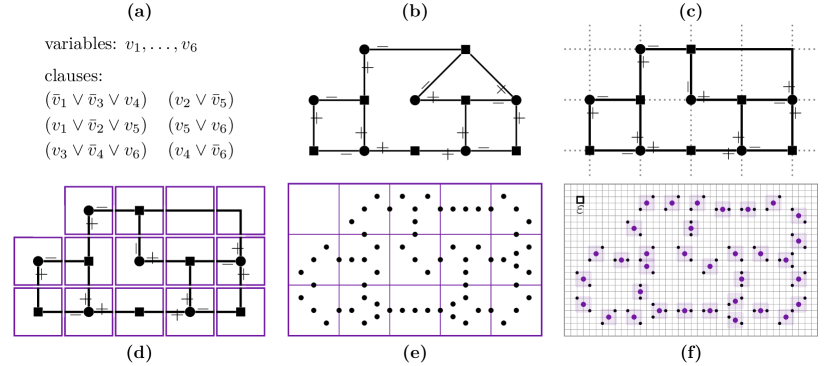
Figure 1: Example of reduction from restricted Boolean satisfiability to Problem UPC. (a) A satisfiable restricted Boolean formula. (b) The formula’s planar bipartite variable–clause invidence graph (circles: variables, squares: clauses, edges: $\pm$ literals). (c) The graph embedded onto an integer grid. (d) The embedding divided into unit tiles of various types. (e) The $h=68$ source points aggregated from each of the tiles. (f) Existence of a $(34,1/8)$-cover of the source points (coloured points are covering points, with uniform neighbourhoods of radius $1/8$ shown). General case in Appendix C.

The following decision problem formalises the task of bounding the proximate rank, or equivalently, detecting nearby low-rank parameters. It is $\mathcal{NP}$-complete by reduction from Problem UPC.

Problem 2 (PR).

Bounding proximate rank (PR) is a decision problem. Each instance comprises a number of hidden units $h\in{\mathbb{N}}$, a parameter $w\in\mathcal{W}_{h}$, a uniform radius $\varepsilon\in{{\mathbb{R}}^{+}}$, and a maximum rank $r\in{\mathbb{N}}$. Affirmative instances are those for which $\operatorname{prank}_{\varepsilon}(w)\leq r$.

Theorem 6.2.

Problem PR is $\mathcal{NP}$-complete.

Proof 2.

Since UPC is $\mathcal{NP}$-complete (Theorem 6.1), it suffices to show $\texttt{UPC}\rightarrow\texttt{PR}$ and $\texttt{PR}\in\mathcal{NP}$.

($\texttt{UPC}\rightarrow\texttt{PR}$, reduction): Given an instance of Problem UPC, allocate one hidden unit per source point, and construct a parameter using the source point coordinates as incoming weights and biases. Actually, to avoid issues with zeros and signs, first translate the source points well into the positive quadrant. Likewise, set the outgoing weights to a positive value. Figure 2 gives an example.

Formally, let $h,r\in{\mathbb{N}}$, $\varepsilon\in{{\mathbb{R}}^{+}}$, and $x_{1},\ldots,x_{h}\in{\mathbb{R}}^{2}$. In linear time construct a PR instance with $h$ hidden units, uniform radius $\varepsilon$, maximum rank $r$, and parameter $w\in\mathcal{W}_{h}$ as follows.

1. Define $x_{\min}=\left(\min_{i=1}^{h}x_{i,1},\min_{i=1}^{h}x_{i,2}\right)\in{\mathbb{R}}^{2}$, containing the minimum first and second coordinates among all source points (minimising over each dimension independently).

2. Define a translation $T:{\mathbb{R}}^{2}\to{\mathbb{R}}^{2}$ such that $T(x)=x-x_{\min}+(2\varepsilon,2\varepsilon)$.

3. Translate the source points ${x_{1},\ldots,x_{h}}$ to ${x^{\prime}_{1},\ldots,x^{\prime}_{h}}$ where $x^{\prime}_{i}=T(x_{i})$. Note (for later) that all components of the translated source points are at least $2\varepsilon$ by step (1).

4. Construct the neural network parameter $w=(2\varepsilon,x^{\prime}_{1,1},x^{\prime}_{1,2},\ldots,2\varepsilon,x^{\prime}_{h,1},x^{\prime}_{h,2},0)\in\mathcal{W}_{h}$. In other words, for $i={{1},\ldots,{h}}$, set $a_{i}=2\varepsilon$, $b_{i}=x^{\prime}_{i,1}$, and $c_{i}=x^{\prime}_{i,2}$; and set $d=0$.

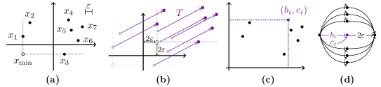
Figure 2: Illustrative example of the parameter construction. (a) A set of source points ${x_{1},\ldots,x_{7}}$. (b) Transformation $T$ translates all points into the positive quadrant by a margin of $2\varepsilon$. (c,d) The coordinates of the transformed points become the incoming weights and biases of the parameter.

($\texttt{UPC}\rightarrow\texttt{PR}$, equivalence): It remains to show that the constructed instance of PR is affirmative if and only if the given instance of UPC is affirmative, that is, there exists an $(r,\varepsilon)$-cover of the source points if and only if the constructed parameter has $\operatorname{prank}_{\varepsilon}(w)\leq r$.

($\Rightarrow$): If there is a small cover of the source points, then the hidden units can be perturbed so that they match up with the (translated) covering points. Since there are few covering points, many units can now be merged, so the original parameter has low proximate rank.

Formally, suppose there exists an $(r,\varepsilon)$-cover ${y_{1},\ldots,y_{r}}$. Define $\rho:{\left\{{1},\ldots,{h}\right\}}\to{\left\{{1},\ldots,{r}\right\}}$ such that the nearest covering point to each source point $x_{i}$ is $y_{\rho(i)}$ (breaking ties arbitrarily). Then for $j={{1},\ldots,{r}}$, define $y^{\prime}_{j}=T(y_{j})$ where $T$ is the translation defined in step (2) of the construction. Finally, define a parameter $w^{\star}=(2\varepsilon,y^{\prime}_{\rho(1),1},y^{\prime}_{\rho(1),2},\ldots,2\varepsilon,y^{\prime}_{\rho(h),1},y^{\prime}_{\rho(h),2},0)\in\mathcal{W}_{h}$ (in other words, for $i={{1},\ldots,{h}}$, $a_{i}^{\star}=2\varepsilon$, $b_{i}^{\star}=y^{\prime}_{\rho(i),1}$, and $c_{i}^{\star}=y^{\prime}_{\rho(i),2}$; and $d^{\star}=0$).

Then $\operatorname{rank}(w^{\star})\leq r$, since there are at most $r$ distinct incoming weight and bias pairs (namely ${y^{\prime}_{1},\ldots,y^{\prime}_{r}}$). Moreover, $\left\|{w-w^{\star}}\right\|_{\infty}\leq\varepsilon$, since both parameters have the same output bias and outgoing weights, and, by the defining property of the cover, for $i={{1},\ldots,{h}}$,

$$\left\|{(b_{i},c_{i})-(b_{i}^{\star},c_{i}^{\star})}\right\|_{\infty}=\left\|{x^{\prime}_{i}-y^{\prime}_{\rho(i)}}\right\|_{\infty}=\left\|{T(x_{i})-T(y_{\rho(i)})}\right\|_{\infty}=\left\|{x_{i}-y_{\rho(i)}}\right\|_{\infty}\leq\varepsilon.$$

Therefore $\operatorname{prank}_{\varepsilon}(w)\leq\operatorname{rank}(w^{\star})\leq r$.

($\Leftarrow$): Conversely, since all of the weights and biases are at least $2\varepsilon$, any nearby low-rank parameter implies the approximate mergeability of some units. Therefore, if the parameter has low proximate rank, there is a small cover of the translated points, and, in turn, of the original points.

Formally, suppose $\operatorname{prank}_{\varepsilon}(w)\leq r$, with $w^{\star}\in\bar{B}_{\infty}\!\left(w;\varepsilon\right)$ such that $\operatorname{rank}(w^{\star})=r^{\star}\leq r$. In general, the only ways that $w^{\star}$ could have reduced rank compared to $w$ are the following (cf. Algorithm 1):

1. Some incoming weight $b_{i}$ could be perturbed to zero, allowing its unit to be eliminated.

2. Two units $i,j$ with $(b_{i},c_{i})$ and $(b_{j},c_{j})$ within $2\varepsilon$ could be perturbed to have identical incoming weight and bias, allowing them to be merged.

3. Two units $i,j$ with $(b_{i},c_{i})$ and $-(b_{j},c_{j})$ within $2\varepsilon$ could be perturbed to have identically negative weight and bias, again allowing them to be merged.

4. Some group of $m\geq 1$ units, merged through the above options, with total outgoing weight within $m\varepsilon$ of zero, could have their outgoing weights perturbed to make the total zero.

By construction, all $a_{i},b_{i},c_{i}\geq 2\varepsilon>0$, immediately ruling out (1) and (3). Option (4) is also ruled out because any such total outgoing weight is $2m\varepsilon>m\varepsilon$. This leaves option (2) alone responsible. Thus, there are exactly $r^{\star}$ distinct incoming weight and bias pairs among the units of $w^{\star}$. Denote these pairs ${y^{\prime}_{1},\ldots,y^{\prime}_{r^{\star}}}$—they constitute an $(r^{\star},\varepsilon)$-cover of the incoming weight and bias vectors of $w$, ${x^{\prime}_{1},\ldots,x^{\prime}_{h}}$ (as $w^{\star}\in\bar{B}_{\infty}\!\left(w;\varepsilon\right)$). Finally, invert $T$ to produce an $(r^{\star},\varepsilon)$-cover of ${x_{1},\ldots,x_{h}}$, and add $r-r^{\star}$ arbitrary covering points to extend this to the desired $(r,\varepsilon)$-cover.

($\texttt{PR}\in\mathcal{NP}$): We must show that an affirmative instance of PR can be verified in polynomial time, given a certificate. Consider an instance $h,r\in{\mathbb{N}}$, $\varepsilon\in{{\mathbb{R}}^{+}}$, and $w=({{{a_{1},b_{1},c_{1}},\ldots,{a_{h},b_{h},c_{h}}}},d)\in\mathcal{W}_{h}$. Use as a certificate a partition ${\Pi_{1},\ldots,\Pi_{J}}$ of ${\left\{\,i\in{\left\{{1},\ldots,{h}\right\}}\,:\,\left\|{b_{i}}\right\|_{\infty}>\varepsilon\,\right\}}$, such that (1) for each $\Pi_{j}$, for each $i,k\in\Pi_{j}$, $\left\|{\operatorname{sign}(b_{i})\cdot(b_{i},c_{i})-\operatorname{sign}(b_{k})\cdot(b_{k},c_{k})}\right\|_{\infty}\leq 2\varepsilon$; and (2) at most $r$ of the $\Pi_{j}$ satisfy $\sum_{i\in\Pi_{j}}\operatorname{sign}(b_{i})\cdot a_{i}>\varepsilon\cdot{\left|\Pi_{j}\right|}$. The validity of such a certificate can be verified in polynomial time by checking each of these conditions directly.

It remains to show that such a certificate exists if and only if the instance is affirmative. If $\operatorname{prank}_{\varepsilon}(w)\leq r$, then there exists a parameter $w^{\star}\in\bar{B}_{\infty}\!\left(w;\varepsilon\right)$ with $\operatorname{rank}(w^{\star})\leq r$. The partition computed from Stage 2 of $\textsc{Compress}(w^{\star})$ satisfies the required properties for $w\in\bar{B}_{\infty}\!\left(w^{\star};\varepsilon\right)$.

Conversely, given such a partition, for each $\Pi_{j}$, define $v_{j}\in{\mathbb{R}}^{2}$ as the centroid of the bounding rectangle of the set of points ${\left\{\,\operatorname{sign}(b_{i})\cdot(b_{i},c_{i})\,:\,i\in\Pi_{j}\,\right\}}$, that is,

$$v_{j}=\frac{1}{2}\left(\max_{i\in\Pi_{j}}\operatorname{sign}(b_{i})\cdot b_{i}+\min_{i\in\Pi_{j}}\operatorname{sign}(b_{i})\cdot b_{i},\ \max_{i\in\Pi_{j}}\operatorname{sign}(b_{i})\cdot c_{i}+\min_{i\in\Pi_{j}}\operatorname{sign}(b_{i})\cdot c_{i}\right)\!.$$

All of the points within these bounding rectangles are at most uniform distance $\varepsilon$ from their centroids. To construct a nearby low-rank parameter, follow the proof of Theorem 5.1 using ${\Pi_{1},\ldots,\Pi_{J}}$ and ${v_{1},\ldots,v_{J}}$ in place of their namesakes from Algorithms 1 and 2. Thus $\operatorname{prank}_{\varepsilon}(w)\leq r$.

7 Discussion

In this paper, we have studied losslessly compressible neural network parameters, measuring the size of a network by the number of hidden units. Losslessly compressible parameters comprise a measure zero subset of the parameter space, but this is a rich subset that stretches throughout the entire parameter space (Farrugia-Roberts, 2023). Moreover, the neighbourhood of this region has nonzero measure and comprises approximately compressible parameters.

It’s possible that part of the empirical success of deep learning can be explained by the proximity of learned neural networks to losslessly compressible parameters. Our theoretical and algorithmic contributions, namely the notions of rank and proximate rank and their associated algorithms, serve as a foundation for future research in this direction. In this section, we outline promising next steps for future work and discuss limitations of our approach.

Limitations of the lossless compressibility framework.

Section 4 offers efficient algorithms for optimal lossless compression and computing the rank of neural network parameters. However, the rank is an idealised notion, serving as a basis for the theory of proximate rank. One would not expect to find compressible parameters in practice, since numerical imprecision is likely to prevent the observation of identically equal, negative, or zero weights in practice. Moreover, the number of units is not the only measure of a network’s description length. For example, the sparsity and precision of weights may be relevant axes of parsimony in neural network modelling.

Returning to the deep learning context—there is a gap between lossless compressibility and phenomena of approximate compressibility. In practical applications and empirical investigations, the neural networks in question are only approximately preserved the function, and moreover the degree of approximation may deteriorate for unlikely inputs. Considering the neighbourhoods of losslessly compressible parameters helps bridge this gap, but there are approximately compressible neural networks beyond the proximity of losslessly compressible parameters, which are not accounted for in this approach. More broadly, a comprehensive account of neural network compressibility must consider architectural redundancy as well as redundancy in the parameter.

Tractable detection of proximity to low-rank parameters.

An important direction for future work is to empirically investigate the proximity of low-rank neural networks to the neural networks that arise during the course of successful deep learning. Unfortunately, our main result (Theorem 6.2) suggests that detecting such proximity is computationally intractable in general, due to the complex structure of the neighbourhoods of low-rank parameters.

There is still hope for empirically investigating the proximate rank of learned networks. Firstly, $\mathcal{NP}$-completeness does not preclude efficient approximation algorithms, and approximations are still useful as a one-sided test of proximity to low-rank parameters. Algorithm 1 provides a naive approximation, with room for improvement in future work. Secondly, Theorem 6.2 is a worst-case analysis—Section 6 essentially constructs pathological parameters poised between nearby low-rank regions such that choosing the optimal direction of perturbation involves solving (a hard instance of) Boolean satisfiability. Such instances might be rare in practice cf. the related problem of $k$-means clustering; Daniely et al., 2012. As an extreme example, detecting proximity to merely compressible parameters ($r=h-1$) permits a polytime solution based on the reducibility conditions.

Towards lossless compressibility theory in modern architectures.

We have studied lossless compressibility in the simple, concrete setting of single-hidden-layer hyperbolic tangent networks. Several elements of our approach will be useful for future work on more modern architectures. At the core of our analysis are structural redundancies arising from zero, constant, or proportional units (cf. reducibility conditions (i)–(iii)). In particular, the computational difficulty of bounding the proximate rank is due to the approximate merging embedding a hard clustering problem. These features are not due to the specifics of the hyperbolic tangent, rather they are generic features of any layer in a feed-forward network component.

In more complex architectures there will be additional or similar opportunities for compression. While unit negation symmetries are characteristic of odd nonlinearities, other nonlinearities will exhibit their own affine symmetries which can be handled analogously. Further redundancies will arise from interactions between layers or from specialised computational structures.

8 Conclusion

Towards a better understanding of complexity and compressibility in learned neural networks, we have developed a theoretical and algorithmic framework for lossless compressibility in single-hidden-layer hyperbolic tangent networks. The rank is a measure of a parameter’s lossless compressibility. Section 4 offers efficient algorithms for performing optimal lossless compression and computing the rank. The proximate rank is a measure of proximity to low-rank parameters. Section 5 offers an efficient algorithm for approximately bounding the proximate rank. In Section 6, we show that optimally bounding the proximate rank, or, equivalently, detecting proximity to low-rank parameters, is $\mathcal{NP}$-complete, by reduction from Boolean satisfiability via a novel hard clustering problem. These results underscore the complexity of losslessly compressible regions of the parameter space and lay a foundation for future theoretical and empirical work on detecting losslessly compressibile parameters arising while learning with more complex architectures.

Appendix A Proofs of algorithm correctness theorems

Here we provide proofs for Theorems 4.1 and 5.1, completing the sketches from the main paper.

See 4.1

Proof 3.

(i): Following the steps of the algorithm we rearrange the summation defining $f_{w}$ to have the form of $f_{w^{\prime}}$. For each $x\in{\mathbb{R}}^{n}$,

$$f_{w}(x) =d+\sum_{i=1}^{h}a_{i}\tanh(b_{i}x+c_{i})$$

$$=d+\sum_{i\notin I}a_{i}\tanh(c_{i})+\sum_{i\in I}a_{i}\tanh(b_{i}x+c_{i})$$ (cf. line 3)

$$=\delta+\sum_{i\in I}a_{i}\tanh(b_{i}x+c_{i})$$ (cf. line 4)

$$=\delta+\sum_{j=1}^{J}\sum_{i\in\Pi_{j}}a_{i}\tanh(b_{i}x+c_{i})$$ (cf. line 6)

$$=\delta+\sum_{j=1}^{J}\sum_{i\in\Pi_{j}}\operatorname{sign}(b_{i})\cdot a_{i}\tanh(\operatorname{sign}(b_{i})\cdot b_{i}x+\operatorname{sign}(b_{i})\cdot c_{i}) \tanh$$ ( odd)

$$=\delta+\sum_{j=1}^{J}\left(\sum_{i\in\Pi_{j}}\operatorname{sign}(b_{i})\cdot a_{i}\right)\tanh(\beta_{j}x+\gamma_{j})$$ (cf. lines 6, 9)

$$=\delta+\sum_{j=1}^{J}\alpha_{j}\tanh(\beta_{j}x+\gamma_{j})$$ (cf. line 8)

$$=\delta+\sum_{j=1}^{r}\alpha_{k_{j}}\tanh(\beta_{k_{j}}x+\gamma_{k_{j}})$$ (cf. line 12)

$$=f_{w^{\prime}}(x).$$ (cf. line 14)

(ii): Each of the reducibility conditions fails to hold for $w^{\prime}\in\mathcal{W}_{r}$: (i) no $\alpha_{k}$ is zero, due to line 12; (ii) no $\beta_{k}$ is zero, due chiefly to line 3; (iii), (iv) all $\pm(\beta_{k},\gamma_{k})$ are distinct, due chiefly to line 6.

See 5.1

Proof 4.

Trace the algorithm to construct a parameter $u\in\bar{B}_{\infty}\!\left(w;\varepsilon\right)$ with $\operatorname{rank}(u)=\textsc{Bound}(\varepsilon,w)$. Construct $u=({{{a^{(u)}_{1},b^{(u)}_{1},c^{(u)}_{1}},\ldots,{a^{(u)}_{h},b^{(u)}_{h},c^{(u)}_{h}}}},d)\in\mathcal{W}_{h}$ as follows.

1. For $i\notin I$, $\left\|{b_{i}}\right\|_{\infty}\leq\varepsilon$, so set $b^{(u)}_{i}=0$, leaving $a^{(u)}_{i}=a_{i}$ and $c^{(u)}_{i}=c_{i}$.

2. For $i\in\Pi_{j}$, note that $\left\|{\operatorname{sign}(b_{i})\cdot(b_{i},c_{i})-v_{j}}\right\|_{\infty}\leq\varepsilon$, so set $(b_{i}^{(u)},c_{i}^{(u)})=\operatorname{sign}(b_{i})\cdot v_{j}$.

3. For $i\in\Pi_{j}$, if $\left\|{\alpha_{j}}\right\|_{\infty}\leq\varepsilon\cdot{\left|\Pi_{j}\right|}$, then set $\displaystyle a_{i}^{(u)}=a_{i}-\operatorname{sign}(b_{i})\cdot\frac{\alpha_{j}}{{\left|\Pi_{j}\right|}}$, else set $a_{i}^{(u)}=a_{i}$.

By construction, $u\in\bar{B}_{\infty}\!\left(w;\varepsilon\right)$. To see that $\operatorname{rank}(u)=\textsc{Bound}(\varepsilon,w)$, run Algorithm 2 on $u$: Stage 1 finds the same $I$, since those $b_{i}^{(u)}=0$. Stage 2 finds the same ${\Pi_{1},\ldots,\Pi_{J}}$, since $\operatorname{sign}(b_{i}^{(u)})\cdot(b_{i}^{(u)},c_{i}^{(u)})=\operatorname{sign}(b_{i})\cdot(b_{i}^{(u)},c_{i}^{(u)})=v_{j}$ ($\operatorname{sign}(b_{i}^{(u)})=\operatorname{sign}(b_{i})$ since the first component of $v_{j}$ is positive, by line 5 of Algorithm 1). Finally, Stage 3 excludes the same $\alpha_{j}$, since for $j$ such that $\left\|{\alpha_{j}}\right\|_{\infty}\leq\varepsilon\cdot{\left|\Pi_{j}\right|}$, these units from $u$ merge into one unit with outgoing weight

$$\sum_{i\in\Pi_{j}}\operatorname{sign}(b_{i}^{(u)})\cdot a_{i}^{(u)}=\sum_{i\in\Pi_{j}}\operatorname{sign}(b_{i})\cdot\left(a_{i}-\operatorname{sign}(b_{i})\cdot\frac{\alpha_{j}}{{\left|\Pi_{j}\right|}}\right)=\sum_{i\in\Pi_{j}}\operatorname{sign}(b_{i})\cdot a_{i}-\alpha_{j}=0.$$

Appendix B Three perspectives on uniform point cover, and related problems

We show that Problem UPC is one of three equivalent perspectives on the same abstract decision problem. Each of the three perspectives suggests distinct connections to existing problems. Figure 3 shows example instances of the three problems.

Perspective 1: Uniform point cover.

Given some points in the plane, is there a small number of new “covering” points so that each (original) point is near a covering point? This is the perspective introduced in the main paper as Problem UPC. It emphasises the existence of covering points, which are useful in the reduction to Problem PR for the proof of Theorem 6.2.

Uniform point cover is reminiscent of well-known hard clustering problems such as Planar $k$-means (Mahajan et al., 2012). The $k$-means problem concerns finding $k$ centroids with a low sum of (squared Euclidean) distances between source points and their nearest centroids. In contrast, uniform point cover concerns finding covering points with a low maximum (uniform) distance between source points and their nearest covering points.

Problem UPC is more similar to the $\mathcal{NP}$-complete problem of absolute vertex $p$-centre (Hakimi, 1964, 1965; Kariv and Hakimi, 1979). This problem concerns finding a set of points on a graph (i.e., vertices or points along edges) with a low maximum (shortest path) distance between vertices and their nearest points in the set. Problem UPC is a geometric $p$-center problem using uniform distances.

A geometric $p$-center problem using Euclidean distances was shown to be $\mathcal{NP}$-complete by Supowit (1981, §4.3.2; see also , ). Megiddo and Supowit (1984) also showed the $\mathcal{NP}$-hardness of an optimisation variant using $L_{1}$ distance (rectilinear or Manhattan distance). We prove that Problem UPC is $\mathcal{NP}$-complete using somewhat similar reductions, but many simplifications afforded by starting from a more restricted variant of Boolean satisfiability.

Perspective 2: Uniform point partition.

Given some points in the plane, can the points be partitioned into a small number of groups with small uniform diameter? This perspective, formalised as Problem UPP, emphasises the grouping of points, rather than the specific choice of covering points.

Consider $h$ points ${x_{1},\ldots,x_{h}}\in{\mathbb{R}}^{2}$. A $(r,\varepsilon)$-partition of the $h$ points is a partition of ${\left\{{1},\ldots,{h}\right\}}$ into $r$ subsets ${\Pi_{1},\ldots,\Pi_{r}}$ such that the uniform distance between points in any subset is at most $\varepsilon$: $\forall k\in\left\{1,\ldots,r\right\}\!,\forall i,j\in\Pi_{k},\left\|{x_{i}-x_{j}}\right\|_{\infty}\leq\varepsilon$.

Problem 3 (UPP).

Uniform point partition (UPP) is a decision problem. Each instance comprises a collection of $h\in{\mathbb{N}}$ points ${x_{1},\ldots,x_{h}}\in{\mathbb{R}}^{2}$, a uniform diameter $\varepsilon\in{{\mathbb{R}}^{+}}$, and a number of groups $r\in{\mathbb{N}}$. Affirmative instances are those for which there exists an $(r,\varepsilon)$-partition of ${x_{1},\ldots,x_{h}}$.

Perspective 3: Clique partition for unit square graphs.

Given a special kind of graph called a unit square graph, can the vertices be partitioned into a small number of cliques? The third perspective strays from the simple neural network context, but reveals further related work.

Consider $h$ points in the plane, ${x_{1},\ldots,x_{h}}\in{\mathbb{R}}^{2}$, and a diameter $\varepsilon\in{{\mathbb{R}}^{+}}$. Thus define an undirected graph $(V,E)$ with vertices $V={\left\{{1},\ldots,{h}\right\}}$ and edges $E={\left\{\,\left\{i,j\right\}\,:\,i\neq j,\left\|{x_{i}-x_{j}}\right\|_{\infty}\leq\varepsilon\,\right\}}$. A unit square graph is any graph that can be constructed in this way. Unit square graphs are a uniform-distance variant of unit disk graphs (based on Euclidean distance; cf. Clark et al., 1990).

Consider an undirected graph $(V,E)$. A clique partition of size $r$ is a partition of the vertices $V$ into $r$ subsets ${\Pi_{1},\ldots,\Pi_{r}}$ such that each subset is a clique: $\forall k\in\left\{1,\ldots,r\right\}\!,\forall v_{i}\neq v_{j}\in\Pi_{k},\left\{v_{i},v_{j}\right\}\in E$.

Problem 4 (usgCP).

Clique partition for unit square graphs (usgCP) is a decision problem. Each instance comprises a unit square graph $(V,E)$ and a number of cliques $r\in{\mathbb{N}}$. Affirmative instances are those for which there exists a clique partition of size $r$.

The clique partition problem is $\mathcal{NP}$-complete in general graphs (Karp, 1972). Cerioli et al. (2004, 2011) showed that it remains $\mathcal{NP}$-complete when restricted to unit disk graphs, using a reduction from a variant of Boolean satisfiability that is somewhat similar to our reduction.

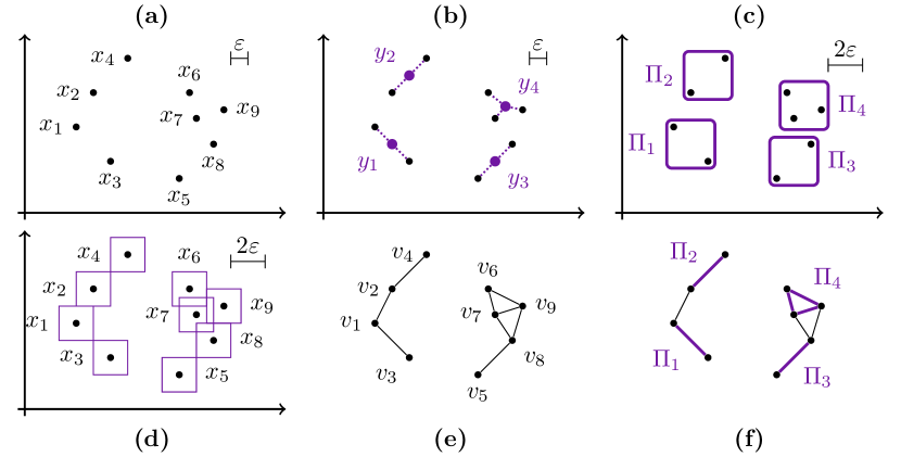
Figure 3: Example instances for Problem UPC, Problem UPP, and Problem usgCP. (a) Nine (source) points ${x_{1},\ldots,x_{9}}$. (b) A $(4,\varepsilon)$-cover ${y_{1},\ldots,y_{4}}$. (c) A $(4,2\varepsilon)$-partition ${\Pi_{1},\ldots,\Pi_{4}}$ ($=\left\{1,3\right\},\left\{2,4\right\},\left\{5,8\right\},\left\{6,7,9\right\}$). (d) The nine points ${x_{1},\ldots,x_{9}}$, along with $2\varepsilon$-width squares. (e) The corresponding unit square graph with vertices ${v_{1},\ldots,v_{9}}$. (f) A partition of the unit square graph into four cliques ${\Pi_{1},\ldots,\Pi_{4}}$. Note: $\varepsilon$ represents a radius in Problem UPC, but a diameter in Problems UPP and usgCP. In these examples, we use $\varepsilon$ for the radius and $2\varepsilon$ for the diameter.

Equivalence of the three perspectives.

Problems UPC, UPP, and usgCP are equivalent in the sense that there is an immediate reduction between any pair of them.

Theorem B.1 (Equivalence of Problems UPC, UPP, and usgCP).

Let $h,r\in{\mathbb{N}}$, $\varepsilon\in{{\mathbb{R}}^{+}}$, and ${x_{1},\ldots,x_{h}}\in{\mathbb{R}}^{2}$. The following conditions are equivalent:

1. there exists an $(r,\frac{1}{2}\varepsilon)$-cover of ${x_{1},\ldots,x_{h}}$;

2. there exists an $(r,\varepsilon)$-partition of ${x_{1},\ldots,x_{h}}$; and

3. the unit square graph on ${x_{1},\ldots,x_{h}}$ (diameter $\varepsilon$) has a clique partition of size $r$.

Proof.

(ii $\Rightarrow$ i): Let ${\Pi_{1},\ldots,\Pi_{r}}$ be an $(r,\varepsilon)$-partition of the points ${x_{1},\ldots,x_{h}}$. For each $\Pi_{j}$, define $y_{j}\in{\mathbb{R}}^{2}$ as the centroid of the bounding rectangle of the set of points ${\left\{\,x_{i}\,:\,i\in\Pi_{j}\,\right\}}$, that is, $y_{j}=\frac{1}{2}\left(\max_{i\in\Pi_{j}}x_{i,1}+\min_{i\in\Pi_{j}}x_{i,1},\ \max_{i\in\Pi_{j}}x_{i,2}+\min_{i\in\Pi_{j}}x_{i,2}\right)$. For each $i\in\Pi_{j}$ and $p\in\left\{1,2\right\}$, let $\alpha=\operatorname{arg\-max}_{a\in\Pi_{j}}x_{a,p}$ and $\beta=\operatorname{arg\-min}_{b\in\Pi_{j}}x_{b,p}$. Then,

$$\operatorname{abs}(2x_{i,p}-2y_{j,p}) =\operatorname{abs}\left(2x_{i,p}-\left(\max_{i\in\Pi_{j}}x_{i,p}+\min_{i\in\Pi_{j}}x_{i,p}\right)\right)$$

$$\leq\operatorname{abs}\left(x_{i,p}-\max_{i\in\Pi_{j}}x_{i,p}\right)+\operatorname{abs}\left(x_{i,p}-\min_{i\in\Pi_{j}}x_{i,p}\right)$$ (triangle inequality)

$$=\max_{i\in\Pi_{j}}x_{i,p}-\min_{i\in\Pi_{j}}x_{i,p} \max_{i\in\Pi_{j}}x_{i,p}\leq x_{i,p}\leq\min_{i\in\Pi_{j}}x_{i,p}$$ ()

$$=x_{\alpha,p}-x_{\beta,p}\leq\left\|{x_{\alpha}-x_{\beta}}\right\|_{\infty}\leq\varepsilon.$$

Thus $\left\|{x_{i}-y_{p}}\right\|_{\infty}\leq\frac{1}{2}\varepsilon$, and ${y_{1},\ldots,y_{k}}$ is an $(r,\frac{1}{2}\varepsilon)$-cover of ${x_{1},\ldots,x_{h}}$.

(i $\Rightarrow$ iii): Let ${y_{1},\ldots,y_{r}}\in{\mathbb{R}}^{2}$ be an $(r,\frac{1}{2}\varepsilon)$-cover of ${x_{1},\ldots,x_{h}}$. Partition $\left\{1,\ldots,h\right\}$ into ${\Pi_{1},\ldots,\Pi_{r}}$ by grouping points according to the nearest covering point (break ties arbitrarily). Then for $i,j\in\Pi_{k}$, $\left\{i,j\right\}\in E$ of the unit square graph, since $\left\|{x_{i}-x_{j}}\right\|_{\infty}\leq\left\|{x_{i}-y_{k}}\right\|_{\infty}+\left\|{y_{k}-x_{j}}\right\|_{\infty}\leq\frac{1}{2}\varepsilon+\frac{1}{2}\varepsilon=\varepsilon$. Thus ${\Pi_{1},\ldots,\Pi_{r}}$ is a clique partition.

(iii $\Rightarrow$ ii): Let ${\Pi_{1},\ldots,\Pi_{r}}$ be a clique partition. Then for $i,j\in\Pi_{k}$, $\left\{i,j\right\}\in E$, and so $\left\|{x_{i}-x_{j}}\right\|_{\infty}\leq\varepsilon$. Thus ${\Pi_{1},\ldots,\Pi_{r}}$ is an $(r,\varepsilon)$-partition. ∎

Appendix C $\mathcal{NP}$-completeness of uniform point cover

In this section, we prove that Problem UPC is $\mathcal{NP}$-complete. By Theorem B.1, it suffices to prove that Problem UPP is $\mathcal{NP}$-complete. This simplifies the presentation of the proof by abstracting away the need to construct specific covering vectors for groups of points. The main part of the proof is a reduction from a restricted variant of Boolean satisfiability, which we call Problem xSAT. Section C.1 introduces Problem xSAT and proves that it is $\mathcal{NP}$-complete. Section C.2 proves that Problem UPP is $\mathcal{NP}$-complete. Appendix D proves the complexity of some problem variants.

C.1 Restricted Boolean satisfiability

Boolean satisfiability is a well-known $\mathcal{NP}$-complete decision problem (Cook, 1971; Levin, 1973). We formalise this problem as follows.

Given $n$ variables, ${v_{1},\ldots,v_{n}}$, a Boolean formula (in conjunctive normal form) is conjunction of $m$ clauses, $c_{1}\land\cdots\land c_{m}$, where each clause is a finite disjunction ($\lor$) of literals, and each literal is either a variable $v_{i}$ or its negation $\bar{v}_{i}$ (called, respectively, a positive occurrence or negative occurrence of the variable $v_{i}$). A truth assignment is a mapping assigning each of the variables ${v_{1},\ldots,v_{n}}$ to the values “true” or “false.” The formula is satisfiable if there exists a truth assignment such that the entire formula evaluates to “true”. That is, each clause contains at least one positive occurrence of a variable assigned “true,” or at least one negative occurrence of a variable assigned “false”.

Problem 5 (SAT).

Boolean satisfiability (SAT) is a decision problem. The instances are all Boolean formulas in conjunctive normal form. Affirmative instances are all satisfiable formulas.

We introduce a variant of Problem SAT, namely Problem xSAT. Let $\phi$ be a Boolean formulas with variables ${v_{1},\ldots,v_{n}}$ and clauses $c_{1}\land\cdots\land c_{m}$. Call $\phi$ a restricted Boolean formula if it meets the following three additional conditions:

1. Each variable $v_{i}$ occurs as a literal in either two clauses or in three clauses. Exactly one of these occurrences is a negative occurrence (the other one or two are positive occurrences).

2. Each clause $c_{j}$ contains either two literals or three literals (these may be any combination of positive and negative).

3. The bipartite variable–clause incidence graph of $\phi$ is a planar graph.

The bipartite variable–clause incidence graph is an undirected graph $(V,E)$ with vertices $V=\left\{v_{1},\ldots,v_{n},c_{1},\ldots,c_{m}\right\}$ and edges $E={\left\{\,\left\{v_{i},c_{j}\right\}\,:\,\text{variable $v_{i}$ occurs as a literal in clause $c_{j}$}\,\right\}}$.

These additional restrictions streamline the proof of Theorem 6.1 in Section C.2, by reducing the complexity of the reduction mapping Boolean formulas to UPP instances.

Problem 6 (xSAT).

Restricted Boolean satisfiability (xSAT) is a decision problem. The instances are all restricted Boolean formulas. Affirmative instances are all satisfiable formulas.

Figure 4 illustrates some instances of Problem xSAT.

Figure 4: Three example restricted Boolean formulas in conjunctive normal form are as follows: $\phi_{1}=(v_{1}\lor v_{2})\land(\bar{v}_{1}\lor v_{2})\land(v_{3}\lor v_{4})\land(\bar{v}_{3}\lor v_{4})\land(\bar{v}_{2}\lor\bar{v}_{4})$; $\phi_{2}=(\bar{v}_{1}\lor v_{2})\land(v_{1}\lor v_{2}\lor\bar{v}_{3})\land(\bar{v}_{2}\lor v_{3})$; and $\phi_{3}=(\bar{v}_{1}\lor\bar{v}_{3}\lor v_{4})\land(v_{1}\lor\bar{v}_{2}\lor v_{5})\land(v_{3}\lor\bar{v}_{4}\lor v_{6})\land(v_{2}\lor\bar{v}_{5})\land(v_{5}\lor v_{6})\land(v_{4}\lor\bar{v}_{6})$. The bipartite variable–clause incidence graphs of the three formulas are depicted above (circles indicate variable vertices, squares indicate clause vertices, positive and negative occurrences (edges) are marked accordingly. Formula $\phi_{1}$ is unsatisfiable whereas formulas $\phi_{2}$ and $\phi_{3}$ are each satisfiable.

Theorem C.1.

Problem xSAT is $\mathcal{NP}$-complete.

Proof 5.

$\texttt{xSAT}\in\mathcal{NP}$ since $\texttt{SAT}\in\mathcal{NP}$. To show $\texttt{SAT}\rightarrow\texttt{xSAT}{}$ much of the work is already done:

1. Cook (1971) reduced SAT to $3$-SAT, a variant with at most three literals per clause.

2. Lichtenstein (1982) extended this reduction to planar $3$-SAT, a variant with at most three literals per clause and a planar bipartite clause–variable incidence graph (in fact the planarity condition studied by Lichtenstein is even stronger).

3. Cerioli et al. (2004, 2011) extended the reduction to planar $3$-SAT${}_{\bar{3}}$—a variant of planar $3$-SAT with at most three occurrences per variable. Cerioli et al. (2004, 2011) used similar techniques to Tovey (1984), Jansen and Müller (1995), and Berman et al. (2003), who studied variants of SAT with bounded occurrences per variable, but no planarity restriction.

It remains to efficiently construct from an instance $\phi$ of planar $3$-SAT${}_{\bar{3}}$ an equisatisfiable formula $\phi^{\prime}$ having additionally (a) at least two occurrences per variable, (b) at least two variables per clause, and (c) exactly one negative occurrence per variable. This can be achieved by removing variables, literals, and clauses and negating occurrences in $\phi$ (noting that such operations do not affect the conditions on $\phi$) as follows. First, establish (a) and (b) by exhaustively applying the following (polynomial-time) operations.

1. If a variable always occurs with one sign (including never or once), remove the variable and all incident clauses. The resulting (sub)formula is equisatisfiable: extend a satisfying assignment by satisfying the removed clauses with the removed variable.

2. If a clause contains a single literal, this variable is determined in a satisfying assignment. Remove the variable and clause along with any other clauses in which the variable occurs with that sign. For other occurrences, retain the clause but remove the literal.¹² If the resulting formula is unsatisfiable, then the additional variable won’t help, and if the resulting formula is satisfiable, then so is the original with the appropriate setting of the variable to satisfy the singleton clause.

Only a polynomial number of operations are possible as each removes one variable. Moreover, thanks to (i), each variable with two occurrences now has one negative occurrence (as required). For variables with three occurrences, one or two are negative. Establish (c) by negating all three occurrences for those that have two negative occurrences (so that the two become positive and the one becomes negative as required). The result is equisatisfiable because satisfying assignments can be translated by negating the truth value assigned to this variable. Carrying out this negation operation for the necessary variables takes polynomial time and completes the reduction.

C.2 Complexity of uniform point partition

Theorem 6.1 is a corollary of Theorem B.1 and the following two results.

Theorem C.2.

$\texttt{UPP}\in\mathcal{NP}$.

Proof 6.

An $(r,\varepsilon)$-partition of the points acts as a certificate. Such a partition can be verified in polynomial time by computing the pairwise uniform distances within each group.

Theorem C.3.

$\texttt{xSAT}\rightarrow\texttt{UPP}$.

Proof 7.

This proof is more substantial. We describe the reduction algorithm in detail, and then formally prove its efficiency and correctness, over the remainder of this section (pages C.3–C.2).

Reduction overview.

Given an xSAT instance, the idea is to build a UPP instance with a collection of points mirroring the structure of the bipartite variable–clause incidence graph of the restricted Boolean formula. To each variable vertex, clause vertex, and edge corresponds a collection of points. The points for each variable vertex can be partitioned in one of two configurations, based on the value of the variable in a truth assignment. Each determines the available groupings of the incident edge’s points so as to propagate these assignments to the clauses. The maximum number of groups is set so that there are enough to include the points of each clause vertex if and only if some variable satisfies that clause in the assignment.

Reduction step 1: Lay out the graph on a grid.

Due to the restrictions on the xSAT instance, the bipartite variable–clause incidence graph is planar with maximum degree three. Therefore there exists a graph layout where (1) the vertices are positioned at integer coordinates, and (2) the edges comprise horizontal and vertical segments between adjacent pairs of integer coordinates (Valiant, 1981, §IV). Moreover, such a (planar, rectilinear, integer) grid layout can be constructed in polynomial time see, e.g., Valiant, 1981; Liu et al., 1998; there is no requirement to produce an “optimal” layout—just a polynomial-time computable layout. Figure 5 shows three examples.

Reduction step 2: Divide the layout into tiles.

The grid layout serves as a blueprint for a UPP instance: it governs how the points corresponding to each variable vertex, clause vertex, and edge are arranged in the plane. The idea is to conceptually divide the plane into unit square tiles, with one tile for each coordinate of the integer grid occupied by a vertex or edge in the grid layout. The tile divisions for the running examples are shown in Figure 5.

Due to the restrictions on xSAT instances, any tile division uses just forty distinct tile types (just nine up to rotation and reflection). There are straight edge segments and corner edge segments, plus clause and variable vertices with two or three edges in any direction, and for variable vertices, exactly one direction corresponds to a negative occurrence. Figure 6 enumerates these types.

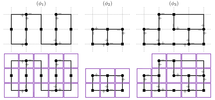
Figure 5: Top: Example planar, rectilinear, integer grid layouts of the bipartite variable–clause incidence graphs from Figure 4. Note: these layouts are computed by hand—those produced by standard algorithms may be larger. Bottom: Division of the same grid layouts into tiles.

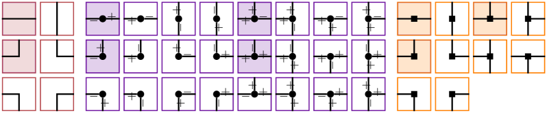
Figure 6: Just forty tile types suffice to construct any tile division of a grid layout. Up to rotation and reflection, just nine distinct types (for example, those highlighted) suffice.

Reduction step 3: Populate the instance with points.

The points of the UPP instance are of two kinds (described in more detail below): (1) boundary points between neighbouring pairs of tiles; and (2) interior points within each tile in a specific arrangement depending on the tile type. The boundary points can be grouped with interior points of one or the other neighbouring tile. In this way, boundary points couple the choice of how to partition the interior points of neighbouring tiles, creating the global constraint that corresponds to satisfiability.

Reduction step 3a: Boundary points between neighbouring tiles.

There is one boundary point at the midpoint of the boundary between each pair of neighbouring tiles. A pair of neighbouring tiles is one for which there is an edge crossing the boundary. It is not sufficient for the tiles to be adjacent. Figure 7 clarifies this distinction using the running examples.

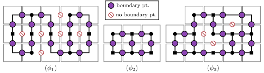
Figure 7: Example of the placement of boundary points between neighbouring tiles. Boundary points are not placed between adjacent tiles if no edge crosses this tile boundary.

Reduction step 3b: Interior points for variable tiles.

Table 1 shows arrangements of interior points for each type of variable tile (up to rotation and reflection). Due to the restrictions on the xSAT instance, each variable tile has one negative boundary point and one or two positive boundary point(s) (corresponding to the variable occurrences). With a given number of groups, the choice of which boundary point(s) to include corresponds to the value of the variable in a truth assignment.

Lemma C.4.

Consider an interior and boundary point arrangement from Table 1 (first 4 rows), or a rectilinear rotation or reflection of such an arrangement. Let $r\in\left\{2,3\right\}$ be the allocated number of groups, and let $\varepsilon\in{{\mathbb{R}}^{+}}$ be the scale.

1. There is no $(k,\varepsilon)$-partition of the interior points if $k<r$.

2. For any $(r,\varepsilon)$-partition of the interior points, the negative boundary point is within uniform distance $\varepsilon$ of all points in some group, if and only if (neither of) the positive boundary point(s) are within uniform distance $\varepsilon$ of all points in any group.

Proof 8.

It suffices to consider the arrangements in Table 1 (first 4 rows) because the uniform distance is invariant to rectilinear rotation and reflection. The claims are then verified by exhaustive consideration of all possible partitions of the interior points into at most $r$ groups.

The partitions indicated in the table are used while constructing a partition of the whole instance given a satisfying assignment. Conversely, no other partitions of the interior points using $r$ groups are possible, except in the fourth row, where other partitions are possible, but, as suffices for the reduction, there are no partitions including both positive and negative boundary points.

Reduction step 3c: Interior points for edge tiles.

Table 1 shows arrangements of interior points for each type of edge tile (up to rotation and reflection). Once the partition of a variable tile includes either the positive boundary point(s) or the negative boundary point, the role of an edge tile is to propagate this choice to the incident clause. These simple point arrangements ensure that the opposite boundary point can be included in a partition of the interior points if and only if the prior boundary point is not (that is, if and only if it was included by the partition of the interior points of the variable tile or, inductively, the previous edge tile).

Lemma C.5.

Consider an interior and boundary point arrangement from Table 1 (last 2 rows), or a rectilinear rotation or reflection of such an arrangement. Let $\varepsilon\in{{\mathbb{R}}^{+}}$ be the scale.

1. There is no $(k,\varepsilon)$-partition of the interior points if $k<2$.

2. For any $(2,\varepsilon)$-partition of the interior points, either boundary point is within uniform distance $\varepsilon$ of all points in some group, if and only if the other boundary point is not within uniform distance $\varepsilon$ of all points in any group.

Proof 9.

Special case of Lemma C.4.

The partitions indicated in Table 1 are the only possible $(2,\varepsilon)$-partitions of the interior points.

Table 1: Arrangement of interior points for variable tiles (first 4 rows) or edge tiles (last 2 rows). $h$ represents the number of interior points (coloured), with nearby boundary points also shown (black). $r$ represents the number of groups allocated to the tile during the reduction.

Reduction step 3d: Interior points for clause tiles.

Table 2 shows arrangements of interior points for each type of clause tile. The arrangements are such that the interior points of the clause tile can be partitioned if and only if one of the boundary points is not included (that is, it must be included by a neighbouring variable or edge tile, indicating the clause will be satisfied by the corresponding literal).

Lemma C.6.

Consider an interior and boundary point arrangement from Table 2, or a rectilinear rotation or reflection of such an arrangement. Let $r\in\left\{2,3\right\}$ be the allocated number of groups, and let $\varepsilon\in{{\mathbb{R}}^{+}}$ be the scale.

1. There is no $(k,\varepsilon)$-partition of the interior points if $k<r$.

2. For any $(r,\varepsilon)$-partition of the interior points, there is at least one boundary point that is not within uniform distance $\varepsilon$ of all points in any group.

Proof 10.

Following Lemma C.4, the conditions can be checked exhaustively.

Table 2 shows the only possible $(r,\varepsilon)$-partitions of the interior points, except in the third row, where a reflected version of the first example partition is also possible.

Table 2: Arrangement of interior points for clause tiles. The number $h$ represents the number of interior points (coloured). The boundary points are also shown (black). The number $r$ represents the number of groups allocated to the tile during the reduction.

Reduction step 4: Set the number of groups.

For the number of groups, total the allocations for the interior points of each tile ($r$ in Tables 1 and 2). That is, set $r$ for the UPP instance to thrice the number of 3-occurrence variables and 3-literal clauses plus twice the number of edge segments, 2-occurrence variables, and 2-literal clauses.

Reduction step 5: Set the uniform diameter.

The reduction works at any (polynomial-time computable) scale. For concreteness, set the diameter to $1/4$, giving each tile unit width.

Formal summary of the reduction.

Given an instance of xSAT, that is, a restricted Boolean formula $\phi$ with variables ${v_{1},\ldots,v_{n}}$ and clauses $c_{1}\land\cdots\land c_{m}$, construct an instance of UPP as described in detail in the above steps. Namely, use the points ${x_{1},\ldots,x_{h}}\in{\mathbb{R}}^{2}$ as described in Reduction step 3 (the interior points from all tiles and the boundary points between neighbouring tiles); a number of groups $r$ as described in Reduction step 4 (the total allocated groups from all of the tiles); and a uniform diameter $\varepsilon=1/4$ as described in Reduction step 5.

Table 3 shows the full UPP instances for the running examples (cf. Figures 4, 5 and 7).

Table 3: Full examples of the reduction from xSAT to UPP, based on xSAT instances described in Figure 4. Exercise: is there an $(r,\varepsilon)$-partition in each case?

Correctness of the reduction.

Step 1 (grid layout) runs in polynomial time (Liu et al., 1998), and the remaining steps run in linear or constant time. It remains to show that the constructed instance of UPP is equivalent to the original xSAT instance. That is, we must show that $\phi$ is satisfiable if and only if there exists an $(r,\varepsilon)$-partition of the points ${x_{1},\ldots,x_{h}}$.

($\Rightarrow$): Suppose $\phi$ is satisfiable. Let $\theta$ be a satisfying truth assignment. Produce an $(r,\varepsilon)$-partition of ${x_{1},\ldots,x_{h}}$ as follows.

1. Partition the interior points of each variable tile as in Table 1. Include the positive boundary point(s) if the variable is assigned “true” in $\theta$, or include the negative boundary point if it is assigned “false”.

2. For each variable tile, follow the included boundary point(s) through zero or more edge tiles to the incident clause’s tile, partitioning the interior points of each edge tile according to Table 1 such that the boundary point in the direction of the clause tile is included.

3. Since $\theta$ is a satisfying assignment, every clause tile is reached in this way at least once, and thus has at least one of its boundary points included in the groups described so far. For each clause tile, partition the interior points according to Table 2, including the remaining boundary points (if any).

4. For each clause tile, follow the remaining boundary points through zero or more edges back to a variable tile, partitioning the interior points of each edge tile according to Table 1 such that the boundary point in the direction of the variable tile is included.

The final step includes exactly the boundary points of variable tiles that were not included in the first step. Thus, all interior and boundary points are included in some group. The number of groups is exactly in accordance with the allocated number of groups per tile, for a total of $r$.

($\Leftarrow$): Suppose there is an $(r,\varepsilon)$-partition of the points. Observe the following:

• Since the interior points of each tile are separated from the tile boundaries by at least $\varepsilon$, no group can include interior points from two separate tiles.

• It follows that the interior points of each tile must be partitioned into their allocated number of groups. If one tile were to use more groups, some other tile would not get its allocation of groups, and it would be impossible to include all of its interior points in the partition (by Lemmas C.4(i), C.5(i), and C.6(i)).

• Since the boundary points have no allocated groups, each boundary point must be included in a group with interior points from one of its neighbouring tiles.

Now, consider each clause tile. By Lemma C.6(ii), there must be at least one boundary point that is included with the interior points of one of its neighbouring tiles. Pick one such direction for each clause and use this to construct a satisfying assignment for $\phi$ as follows.

In each direction, follow the sequence of zero or more edge tiles back to a variable tile. By Lemma C.5(ii), each boundary point along the sequence of edges must be included with the interior points of the next edge tile in the sequence. In turn, the boundary point at the variable tile must be included with the interior points of the variable tile. If this is a positive boundary point, set this variable to “true” in a truth assignment $\theta$, and if it is a negative boundary point, set the variable to “false”.

This uniquely defines the truth assignment $\theta$ for all variables reached in this way at least once. If a variable is reached this way from two separate clauses, it must be through its two positive boundary points, since by Lemma C.4(ii), it is impossible for the partition to have both a negative and a positive boundary point included with the interior points of the variable tile. Since some variables may not be reached at all in this way, $\theta$ is not completely defined. Complete the definition of $\theta$ by assigning arbitrary truth values to such variables.

The truth assignment $\theta$ is a satisfying assignment for $\phi$. Each clause is satisfied by at least one literal, corresponding to the variable tile that was reached through one of the clause tile’s boundary points not grouped with the clause tile’s interior points in the partition.

This concludes the proof of Theorem C.3.

Appendix D Problem variations and their computational complexity

In this section we discuss several minor variations of Problem UPC.

Uniform vector partition is hard.

Consider a generalisation of Problem UPC beyond the plane, as follows. Let $p\in{\mathbb{N}^{+}}$. Given $h$ source vectors ${x_{1},\ldots,x_{h}}\in{\mathbb{R}}^{p}$, define an $(r,\varepsilon)$-cover, a list of $r$ covering vectors ${y_{1},\ldots,y_{r}}\in{\mathbb{R}}^{p}$ such that the uniform distance between each source vector and its nearest covering vector is at most $\varepsilon$ (that is, $\forall i\in\left\{1,\ldots,h\right\}\!,\exists j\in\left\{1,\ldots,r\right\}\!,\left\|{x_{i}-y_{j}}\right\|_{\infty}\leq\varepsilon$).

Problem 7 ($\texttt{UVC}^{p}$).

Let $p\in{\mathbb{N}^{+}}$. Uniform vector cover in ${\mathbb{R}}^{p}$ ($\texttt{UVC}^{p}$) is a decision problem. Each instance comprises a collection of $h\in{\mathbb{N}}$ source points ${x_{1},\ldots,x_{h}}\in{\mathbb{R}}^{p}$, a uniform radius $\varepsilon\in{{\mathbb{R}}^{+}}$, and a number of covering points $r\in{\mathbb{N}}$. Affirmative instances are those for which there exists an $(r,\varepsilon)$-cover of ${x_{1},\ldots,x_{h}}$.

Theorem D.1.

If $p\geq 2$, then $\texttt{UVC}^{\,p}$ is $\mathcal{NP}$-complete.

Proof 11.

($\texttt{UPC}\rightarrow\texttt{UVC}^{p}$): Let $p\geq 2$. Embed the source points from the UPC instance into the first two dimensions of ${\mathbb{R}}^{p}$ (leaving the remaining components zero). If there is an $(r,\varepsilon)$-cover of the 2-dimensional points, embed it similarly to derive a $p$-dimensional $(r,\varepsilon)$-cover. Conversely, if there is a $p$-dimensional $(r,\varepsilon)$-cover, truncate it to the first two dimensions to derive an $(r,\varepsilon)$-cover.

($\texttt{UVC}^{p}\in\mathcal{NP}$): Use an $(r,2\varepsilon)$-partition (suitably generalised to $p$ dimensions) as a polynomial-time verifiable certificate. Such a certificate is appropriate along the lines of the proof of Theorem B.1. (An arbitrary $(r,\varepsilon)$-cover is unsuitable as a certificate along the lines of Footnote 9.)

Remark D.2.

By a $p$-dimensional generalisation of Theorem B.1, $p$-dimensional generalisations of Problem UPP and Problem usgCP are also $\mathcal{NP}$-complete for $p\geq 2$.

Uniform scalar partition is easy.

On the other hand, $\texttt{UVC}^{1}$, which could be called uniform scalar cover, is in $\mathcal{P}$. A minimal cover can be constructed using a greedy algorithm with runtime ${\mathcal{O}}(h\log h)$. An $(r,\varepsilon)$-cover exists if and only if there are at most $r$ scalars in the result.

Algorithm 1 (Optimal uniform scalar cover).

Proceed:

UniformScalarCover$h\in{\mathbb{N}}$, $\varepsilon\in{{\mathbb{R}}^{+}}$, ${x_{1},\ldots,x_{h}}\in{\mathbb{R}}$

1:${x^{\prime}_{1},\ldots,x^{\prime}_{h}}\leftarrow{x_{1},\ldots,x_{h}}$, sorted in non-decreasing order.

2:$j\leftarrow 0$ $i={{1},\ldots,{h}}$ $j=0$ or $x^{\prime}_{i}>y_{j}+\varepsilon$

3:$j\leftarrow j+1$

4:$y_{j}\leftarrow x^{\prime}_{i}+\varepsilon$

5:${y_{1},\ldots,y_{j}}$

Theorem D.3 (Algorithm 1 correctness).

Let $h\in{\mathbb{N}}$, $\varepsilon\in{{\mathbb{R}}^{+}}$, and ${x_{1},\ldots,x_{h}}\in{\mathbb{R}}$. Let ${y_{1},\ldots,y_{r}}=\textsc{UniformScalarCover}(h,\varepsilon,{x_{1},\ldots,x_{h}})$. Then (i) ${y_{1},\ldots,y_{r}}$ is an $(r,\varepsilon)$-cover of ${x_{1},\ldots,x_{h}}$; and (ii) no $(k,\varepsilon)$-cover exists for $k<r$.

Proof 12.

(i): After each iteration $i={{1},\ldots,{h}}$, if the if branch was entered, then $\left\|{x^{\prime}_{i}-y_{j}}\right\|_{\infty}=\left\|{x^{\prime}_{i}-(x^{\prime}_{i}+\varepsilon)}\right\|_{\infty}=\varepsilon$. If not, that is, if $x^{\prime}_{i}\leq y_{j}+\varepsilon$, let $k$ be the last iteration in which $j$ was increased. Then $x^{\prime}_{i}\geq x^{\prime}_{k}=y_{j}-\varepsilon$. In summary, $y_{j}-\varepsilon\leq x^{\prime}_{i}\leq y_{j}+\varepsilon$, as required.

(ii): For $j={{1},\ldots,{r}}$, let $\xi_{j}=x^{\prime}_{i}$ from the iteration in which $y_{j}$ was defined. Then for $j\neq k$, $\left\|{\xi_{j}-\xi_{k}}\right\|_{\infty}\geq 2\varepsilon$. No covering scalar could be within distance $\varepsilon$ of any two of these source scalars. Thus at least $r$ covering scalars are required to cover ${\xi_{1},\ldots,\xi_{r}}$, and, in turn, ${x_{1},\ldots,x_{h}}$.

Clique partition on ‘square penny’ graphs is hard.

Cerioli et al. (2004, 2011) showed that clique partition is $\mathcal{NP}$-complete in a restricted variant of of unit disk graphs called penny graphs. A penny graph is a unit disk graph in which the Euclidean distance between source points is at least $\varepsilon$, evoking the contact relationships among non-overlapping circular coins.

Our reduction (Appendix C) happens to produce a set of source points for a unit square graph satisfying a uniform distance version of this condition. Therefore, our proof shows that clique partition remains $\mathcal{NP}$-complete in this special family of graphs as well.

Appendix E A characterisation of the class of bounded-rank parameters

We offer a characterisation of the subset of parameter space with parameters of a given maximum rank. These are the subsets to which detecting proximity is proved $\mathcal{NP}$-complete in Theorem 6.2.

Let $r,h\in{\mathbb{N}}$ with $r\leq h$. The bounded rank region of rank $r$ is the subset of parameters of rank at most $r$, $\mathfrak{B}_{r}={\left\{\,w\in\mathcal{W}_{h}\,:\,\operatorname{rank}(w)\leq r\,\right\}}\subseteq\mathcal{W}_{h}$. The key to characterising bounded rank regions is that for each parameter in $\mathfrak{B}_{r}$, at least $h-r$ units would be removed during lossless compression. Considering the various possible ways in which units can be removed in the course of Algorithm 1 leads to a characterisation of the bounded rank region as a union of linear subspaces.

To this end, let $H={\left\{{1},\ldots,{h}\right\}}$, and define a compression trace on $h$ units as a 4-tuple $(\bar{I},\Pi,\bar{K},\sigma)$ where $\bar{I}\subseteq H$ is a subset of units (conceptually, those to be removed in Stage 1), $\Pi={\Pi_{1},\ldots,\Pi_{J}}$ is a partition of $H\setminus\bar{I}$ (the remaining units) into $J$ groups (to be merged in Stage 2), $\bar{K}\subseteq{\left\{{1},\ldots,{J}\right\}}$ (merged units removed in Stage 3), and $\sigma\in\left\{-1,+1\right\}^{h}$ is a sign vector (unit orientations for purposes of merging). The length of the compression trace $(\bar{I},\Pi,\bar{K},\sigma)$ on $h$ units is $J-{\left|\bar{K}\right|}$ (representing the number of units remaining). A compression trace of length $r$ thus captures the notion of a “way in which $h-r$ units can be removed in the course of Algorithm 1”.

Theorem E.1.

Let $r\leq h\in{\mathbb{N}}$. The bounded rank region $\mathfrak{B}_{r}\subseteq\mathcal{W}_{h}$ is a union of linear subspaces

$$\mathfrak{B}_{r}=\bigcup_{(\bar{I},\Pi,\bar{K},\sigma)\in\Xi(h,r)}\left(\bigcap_{i\in\bar{I}}S^{(1)}_{i}\cap\bigcap_{j=1}^{J}S^{(2)}_{\Pi_{j},\sigma}\cap\bigcap_{k\in\bar{K}}S^{(3)}_{\Pi_{k},\sigma}\right)$$ (1)

where $\Xi(h,r)$ denotes the set of all compression traces on $h$ units with length $r$;

$$S^{(1)}_{i} ={\left\{\,({{{a_{1},b_{1},c_{1}},\ldots,{a_{h},b_{h},c_{h}}}},d)\in\mathcal{W}_{h}\,:\,b_{i}=0\,\right\}};$$

$$S^{(2)}_{\Pi,\sigma} ={\left\{\,({{{a_{1},b_{1},c_{1}},\ldots,{a_{h},b_{h},c_{h}}}},d)\in\mathcal{W}_{h}\,:\,\forall i,j\in\Pi,\,\sigma_{i}b_{i}=\sigma_{j}b_{j}\land\sigma_{i}c_{i}=\sigma_{j}c_{j}\,\right\}};\text{ and}$$

$$S^{(3)}_{\Pi,\sigma} ={\left\{\,({{{a_{1},b_{1},c_{1}},\ldots,{a_{h},b_{h},c_{h}}}},d)\in\mathcal{W}_{h}\,:\,\textstyle\sum_{i\in\Pi}\sigma_{i}a_{i}=0\,\right\}}.$$

Proof 13.

($\supseteq$): Suppose $w=({{{a_{1},b_{1},c_{1}},\ldots,{a_{h},b_{h},c_{h}}}},d)\in\mathcal{W}_{h}$ is in the union in (1), and therefore in the intersection for some compression trace $(\bar{I},\Pi,\bar{K},\sigma)$. The constraints imposed on $w$ by membership in this intersection imply that the network is compressible:

1. For $i\in\bar{I}$, since $w\in S^{(1)}_{i}$, $b_{i}=0$, so unit $i$ can be removed.

2. For $j={{1},\ldots,{J}}$, since $w\in S^{(2)}_{\Pi_{j},\sigma}$, the units in $\Pi_{j}$ can be merged together.

3. For $k\in\bar{K}$, since $w\in S^{(3)}_{\Pi_{k},\sigma}$, merged unit $k$ has outgoing weight $0$ and can be removed.

It follows that there is a parameter with $J-{\left|\bar{K}\right|}$ units that is functionally equivalent to $w$. Therefore $\operatorname{rank}(w)\leq J-{\left|\bar{K}\right|}=r$ and $w\in\mathfrak{B}_{r}$.

($\subseteq$): Conversely, suppose $w\in\mathfrak{B}_{r}$. Construct a compression trace following $\textsc{Compress}(w)$. First, set $\sigma_{i}=\operatorname{sign}(b_{i})$ where $b_{i}\neq 0$ (if $b_{i}=0$, set $\sigma_{i}=\pm 1$ arbitrarily, this has no effect). Then:

1. Set $\bar{I}={\left\{{1},\ldots,{h}\right\}}\setminus I$ where $I$ is computed on line 3. It follows that for $i\in\bar{I}$, $w\in S^{(1)}_{i}$.

2. Set $\Pi$ to the partition computed on line 6. It follows that for $j={{1},\ldots,{J}}$, $w\in S^{(2)}_{\Pi_{j},\sigma}$.

3. Set $\bar{K}={\left\{\,j\in{\left\{{1},\ldots,{J}\right\}}\,:\,\alpha_{j}=0\,\right\}}$ (cf. lines 8,12). Thus for $k\in\bar{K}$, $w\in S^{(3)}_{\Pi_{k},\sigma}$.

By construction $w$ is in $\bigcap_{i\in\bar{I}}S^{(1)}_{i}\cap\bigcap_{j=1}^{J}S^{(2)}_{\Pi_{j},\sigma}\cap\bigcap_{k\in\bar{K}}S^{(3)}_{\Pi_{k},\sigma}$. However, the compression trace $(\bar{I},\Pi,\bar{K},\sigma)$ has length $\operatorname{rank}(w)\leq r$. If $\operatorname{rank}(w)<r$, remove constraints on $r-\operatorname{rank}(w)$ units by some combination of the following operations: (1) remove one unit from $\bar{I}$ (add it as singleton group to $\Pi$), (2) remove one unit from a non-singleton group in $\Pi$ (add it back to $\Pi$ as a singleton group), and/or (3) remove one merged unit from $\bar{K}$. None of these operations add nontrivial constraints on $w$, so it’s still the case that $w$ is in the intersection for the modified compression trace. However, now the length of the compression trace is $r$, so it follows that $w$ is in the union as required.

Appendix F Some additional properties of the proximate rank

We document some additional basic properties of the proximate rank.

Variation with uniform radius.

Fix $w\in\mathcal{W}_{h}$. Then $0\leq\operatorname{prank}_{\varepsilon}(w)\leq\operatorname{rank}(w)$, depending on $\varepsilon$. The following proposition demonstrates some basic properties of this relationship.

Proposition F.1.

Let $h\in{\mathbb{N}}$. Fix $w\in\mathcal{W}_{h}$ and consider $\operatorname{prank}_{\varepsilon}(w)$ as a function of $\varepsilon$. Then,

1. $\operatorname{prank}_{\varepsilon}(w)$ is antitone in $\varepsilon$: if $\varepsilon\geq\varepsilon^{\prime}$ then $\operatorname{prank}_{\varepsilon}(w)\leq\operatorname{prank}_{\varepsilon^{\prime}}(w)$; and

2. $\operatorname{prank}_{\varepsilon}(w)$ is right-continuous in $\varepsilon$: $\lim_{\delta\to 0^{+}}\operatorname{prank}_{\varepsilon+\delta}(w)=\operatorname{prank}_{\varepsilon}(w)$.

Proof 14.

For (i), put $u\in\bar{B}_{\infty}\!\left(w;\varepsilon^{\prime}\right)$ such that $\operatorname{rank}(u)=\operatorname{prank}_{\varepsilon^{\prime}}(w)$. Then $u\in\bar{B}_{\infty}\!\left(w;\varepsilon\right)$, so $\operatorname{prank}_{\varepsilon^{\prime}}(w)=\operatorname{rank}(u)\geq\operatorname{prank}_{\varepsilon}(w)$. Then for (ii), since $\operatorname{prank}_{\varepsilon}(w)\leq\operatorname{rank}(w)$ the limit exists by the monotone convergence theorem. Proceed to bound $\operatorname{prank}_{\varepsilon}(w)$ above and below by $r=\lim_{\delta\to 0^{+}}\operatorname{prank}_{\varepsilon+\delta}(w)$. For the lower bound, for $\delta\in{{\mathbb{R}}^{+}}$, $\operatorname{prank}_{\varepsilon+\delta}(w)\leq\operatorname{prank}_{\varepsilon}(w)$ by (i), so $r=\lim_{\delta\to 0^{+}}\operatorname{prank}_{\varepsilon+\delta}(w)\leq\operatorname{prank}_{\varepsilon}(w)$.

For the upper bound, since the proximate rank is a natural number, the limit is achieved for some positive $\delta$. That is, $\exists\Delta\in{{\mathbb{R}}^{+}}$ such that $\operatorname{prank}_{\varepsilon+\Delta}(w)=r$. Then for $k=1,2,\ldots$ put $u_{k}\in\bar{B}_{\infty}\!\left(w;\varepsilon+\Delta/k\right)$ with $\operatorname{rank}(u_{k})=r$. Since $\bar{B}_{\infty}\!\left(w;\varepsilon+\Delta\right)$ is compact the sequence $u_{1},u_{2},\ldots$ has an accumulation point—call it $u$. Now, since $u_{1},u_{2},\ldots\in\mathfrak{B}_{r}$ (parameters of rank at most $r$, Appendix E), a closed set (by Theorem E.1), the accumulation point $u\in\mathfrak{B}_{r}$. Thus, $\operatorname{rank}(u)\leq r$. Finally, $u\in\bigcap_{k=1}^{\infty}\bar{B}_{\infty}\!\left(w;\varepsilon+\Delta/k\right)=\bar{B}_{\infty}\!\left(w;\varepsilon\right)$, so $r\geq\operatorname{rank}(u)\geq\operatorname{prank}_{\varepsilon}(w)$.

A similar proof implies that $\operatorname{prank}_{\varepsilon}(w)$ achieves its upper bound $\operatorname{rank}(w)$ for small enough $\varepsilon>0$. The lower bound $0$ is also achieved; for example for $\varepsilon\geq\left\|{w}\right\|_{\infty}=\left\|{w-0}\right\|_{\infty}$.

Variation with functionally equivalent parameters.

The rank of $w\in\mathcal{W}_{h}$ is defined in terms of $f_{w}$, so functionally equivalent parameters have the same rank. This is not necessarily the case for the proximate rank—consider Example F.2. Similar counterexamples hold if a non-uniform metric is used. This is a consequence of the fundamental observation that functionally equivalent parameters may have rather different parametric neighbourhoods.

Example F.2.

Let $\varepsilon\in{{\mathbb{R}}^{+}}$. Consider the neural network parameters $w,w^{\prime}\in\mathcal{W}_{2}$ with $w=(2\varepsilon,2\varepsilon,0,0,0,0,0)$ and $w^{\prime}=(2\varepsilon,2\varepsilon,0,5\varepsilon,0,0,0)$. Then for $x\in{\mathbb{R}}$,

$$f_{w}(x) =0+2\varepsilon\tanh(2\varepsilon x+0)+0\tanh(0x+0)$$

$$=0+2\varepsilon\tanh(2\varepsilon x+0)+0\tanh(5\varepsilon x+0)=f_{w^{\prime}}(x),$$

but $\operatorname{prank}_{\varepsilon}(w)=\operatorname{rank}(\varepsilon,\varepsilon,0;-\varepsilon,\varepsilon,0;0)=0\neq 1=\operatorname{prank}_{\varepsilon}(w^{\prime})$.

However, functionally equivalent incompressible parameters have the same proximate rank.

Proposition F.3.

Let $h\in{\mathbb{N}}$. Consider a permutation $\pi\in S_{h}$ and a sign vector $\sigma\in\left\{-1,+1\right\}^{h}$. Define $T_{\pi,\sigma}:\mathcal{W}_{h}\to\mathcal{W}_{h}$ such that

$$T_{\pi,\sigma}({{{a_{1},b_{1},c_{1}},\ldots,{a_{h},b_{h},c_{h}}}},d)=(\sigma_{1}a_{\pi(1)},\sigma_{1}b_{\pi(1)},\sigma_{1}c_{\pi(1)},\ldots,\sigma_{h}a_{\pi(h)},\sigma_{h}b_{\pi(h)},\sigma_{h}c_{\pi(h)},d).$$

Then for $w\in\mathcal{W}_{h},\varepsilon\in{{\mathbb{R}}^{+}}$, $\operatorname{prank}_{\varepsilon}(w)=\operatorname{prank}_{\varepsilon}(T_{\pi,\sigma}(w^{\prime}))$.

Proof 15.

$T_{\pi,\sigma}:\mathcal{W}_{h}\to\mathcal{W}_{h}$ is an isometry with respect to the uniform distance, so

$$\bar{B}_{\infty}\!\left(T_{\pi,\sigma}(w);\varepsilon\right)={\left\{\,T_{\pi,\sigma}(u)\,:\,u\in\bar{B}_{\infty}\!\left(w;\varepsilon\right)\,\right\}}.$$

Moreover, $T_{\pi,\sigma}$ is a symmetry of the parameter–function map (Chen et al., 1993), so it preserves the implemented function and therefore the rank of the parameters in the neighbourhood.

Corollary F.4.

Let $h\in{\mathbb{N}}$. Consider two incompressible (minimal) parameters $w,w^{\prime}\in\mathcal{W}_{h}$ and a uniform radius $\varepsilon\in{{\mathbb{R}}^{+}}$. If $f_{w}=f_{w^{\prime}}$ then $\operatorname{prank}_{\varepsilon}(w)=\operatorname{prank}_{\varepsilon}(w^{\prime})$.

Proof 16.

Since $w,w^{\prime}$ are functionally equivalent and incompressible (minimal), they are related by a permutation transformation and a negation transformation (Sussmann, 1992).

Appendix G Bounding proximate rank with biasless units is still hard

In this appendix, we consider a simpler neural network architecture with unbiased hidden units (such that unit clustering takes place in one dimension). In the main paper we proved the hardness of Problem PR using a reduction from Problem UPC, a planar clustering problem. While a one-dimensional variant of Problem UPC is in $\mathcal{P}$ (Appendix D), we show that in a biasless architecture, bounding proximate rank is still $\mathcal{NP}$-complete, by reduction from a subset sum problem.

This biasless architecture is of limited practical interest—rather, it provides a minimal illustration of a “second layer of complexity” in computing the proximate rank. Roughly: computing an optimal approximate partition of the units alone is not sufficient—one must seek an approximate partition that jointly maximises the numbers of units that can be eliminated (1) by approximate merging and (2) with total outgoing weight near zero (cf. Algorithm 1). The reduction of subset sum to bounding proximate rank in biasless networks is chiefly based on objective (2). The reduction is not specific to biasless networks—a similar reduction is possible for biased architectures.

Biasless hyperbolic tangent networks.

Formally, consider an architecture with one input unit, one biased output unit, and one hidden layer of $h\in{\mathbb{N}}$ unbiased hidden units with the hyperbolic tangent nonlinearity. The weights of the network are encoded in a parameter vector in the format $u=(a_{1},b_{1},\ldots,a_{h},b_{h})\in\mathcal{U}_{h}={\mathbb{R}}^{2h}$, where for each hidden unit $i={{1},\ldots,{h}}$ there is an outgoing weight $a_{i}\in{\mathbb{R}}$ and an incoming weight $b_{i}\in{\mathbb{R}}$. Thus each parameter $u\in\mathcal{U}_{h}$ indexes a mathematical function $f_{u}:{\mathbb{R}}\to{\mathbb{R}}$ such that $f_{u}(x)=\sum_{i=1}^{h}a_{i}\tanh(b_{i}x)$.

The notions of functional equivalence, lossless compressibility, rank, and proximate rank from the main paper generalise straightforwardly to this setting. The analogous reducibility conditions are:

1. $a_{i}=0$ for some $i$, or

2. $b_{i}=0$ for some $i$, or

3. $b_{i}=b_{j}$ for some $i\neq j$, or

4. $b_{i}=-b_{j}$ for some $i\neq j$.

Proper subset sum zero.

The subset sum problem concerns finding a subset of a collection of positive integers with a given sum (Karp, 1972; Garey and Johnson, 1979).

Problem 8 (SSum).

Subset sum (SSum) is a decision problem. Each instance comprises a collection of $n\in{\mathbb{N}^{+}}$ positive integers, ${x_{1},\ldots,x_{n}}\in{\mathbb{N}^{+}}$ and a target integer $T\in{\mathbb{N}^{+}}$. Affirmative instances are those for which there exists a subset $S\subseteq{\left\{{1},\ldots,{n}\right\}}$ such that $\sum_{i\in S}x_{i}=T$.

Theorem G.1 (Karp, 1972; Garey and Johnson, 1979).

Problem SSum is $\mathcal{NP}$-complete.

We pursue a reduction to Problem PR-b from the following $\mathcal{NP}$-complete variant:

Problem 9 (SSZ).

Proper subset sum zero (SSZ) is a decision problem. Each instance comprises a collection of $n\in{\mathbb{N}^{+}}$ positive or negative integers, ${x_{1},\ldots,x_{n}}\in\mathbb{Z}\setminus\left\{0\right\}$. Affirmative instances are those for which there exists a non-empty, proper subset $S\subsetneq{\left\{{1},\ldots,{n}\right\}}$ such that $\sum_{i\in S}x_{i}=0$.

Theorem G.2.

Problem SSZ is $\mathcal{NP}$-complete.

Proof 17.

($\texttt{SSZ}\in\mathcal{NP}$): The subset $S$ serves as its own certificate. Its validity can be verified in polynomial time by checking that $\left\{\right\}\subsetneq S\subsetneq{\left\{{1},\ldots,{n}\right\}}$ and $\sum_{i\in S}x_{i}=0$.

($\texttt{SSum}\rightarrow\texttt{SSZ}$): Consider an SSum instance with collection ${x_{1},\ldots,x_{n}}{\mathbb{N}^{+}}$ and target $T\in{\mathbb{N}^{+}}$. First, rule out the case $\sum{i=1}^{n}x_{i}=T$ (if so, return a trivial affirmative instance of SSZ). Otherwise, let $x_{n+1}=-T$ and return the SSZ instance with collection ${x_{1},\ldots,x_{n+1}}\in\mathbb{Z}\setminus\left\{0\right\}$. Now, consider an affirmative instance of SSum with subset $S\subseteq{\left\{{1},\ldots,{n}\right\}}$. If $S={\left\{{1},\ldots,{n}\right\}}$ then the new instance is affirmative by construction. Otherwise, $S^{\prime}=S\cup\left\{n+1\right\}$ is a non-empty, proper subset of ${\left\{{1},\ldots,{n+1}\right\}}$ such that $\sum_{i\in S^{\prime}}x_{i}=\left(\sum_{i\in S}x_{i}\right)-T=0$. Conversely, if the constructed instance is affirmative (aside from in the trivial case) with subset $S^{\prime}$, then $n+1\in S^{\prime}$ since ${x_{1},\ldots,x_{n}}>0$. It follows that $S=S^{\prime}\setminus\left\{n+1\right\}$ satisfies $\sum_{i\in S}x_{i}=\left(\sum_{i\in S^{\prime}}x_{i}\right)-x_{n+1}=0-(-T)=T$.

Complexity of unbiased proximate rank.

We formalise the problem of bounding the proximate rank in the biasless architecture as follows.

Problem 10 (PR-b).

Bounding biasless proximate rank (PR-b) is a decision problem. Each instance comprises a number of hidden units $h\in{\mathbb{N}}$, a parameter $u\in\mathcal{U}_{h}$, a uniform radius $\varepsilon\in{{\mathbb{R}}^{+}}$, and a maximum rank $r\in{\mathbb{N}}$. Affirmative instances are those for which $\operatorname{prank}_{\varepsilon}(u)\leq r$.

Theorem G.3.

Problem PR-b is $\mathcal{NP}$-complete.

Proof 18.

Since SSZ is $\mathcal{NP}$-complete (Theorem G.2), it suffices to show $\texttt{SSZ}\rightarrow\texttt{PR-b}$ and $\texttt{PR-b}\in\mathcal{NP}$.

($\texttt{SSZ}\rightarrow\texttt{PR-b}$, reduction): Consider an instance of Problem SSZ with ${x_{1},\ldots,x_{n}}\in\mathbb{Z}\setminus\left\{0\right\}$. Construct an instance of Problem PR-b in ${\mathcal{O}}(n^{2})$ time as follows (see Figure 8 for an example). Set $h=n^{2}$, conceptually dividing the $n^{2}$ hidden units into $n$ groups of $n$ units. Construct a parameter

$$u =(a_{1,1},b_{1,1},\ldots,a_{1,n},b_{1,n},a_{2,1},b_{2,1},\ldots,a_{n,n},b_{n,n})\in\mathcal{U}_{n^{2}},$$

where for each unit $$j={{1},\ldots,{n}} i={{1},\ldots,{n}}$$ of each unit group :

$$a_{i,j} =n\cdot x_{\operatorname{mod}(i+j-1,n)},$$

$$b_{i,j} =(2i-1)+\frac{j-1}{n-1}.$$

That is, the outgoing weights for units in group $i$ are just the collection ${x_{1},\ldots,x_{n}}$ cycled to start from $x_{i}$, and scaled by a factor of $n$; and the incoming weights for units in group $i$ are evenly spaced values in the interval from $2i-1$ to $2i$.

Moreover, set $\varepsilon=\frac{1}{2}\frac{n-2}{n-1}$, such that an interval of width $2\varepsilon$ can cover $n-1$ of the incoming weights from any group, but not all $n$, and no two units from different groups. Finally, set $r=2n-1$, that is, one less than enough to allocate two compressed units to each of the $n$ groups.

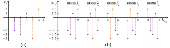
Figure 8: Illustrative example of the parameter construction. (a) A Problem SSZ instance with collection ${x_{1},\ldots,x_{5}}=-3,-4,1,-5,2$. (b) Scatter plot of the incoming and outgoing weights of the $5$ groups of $5$ units of the constructed parameter $u\in\mathcal{U}_{25}$. Moreover, $\varepsilon=3/8$ and $r=9$.

($\texttt{SSZ}\rightarrow\texttt{PR-b}$, equivalence): It remains to show that the constructed instance of PR-b is affirmative if and only if the given instance of SSZ is affirmative, that is, there exists a nonempty proper subset with zero sum if and only if the constructed parameter has $\operatorname{prank}_{\varepsilon}(u)\leq r$. They key idea is that a nearby sufficiently-compressible parameter must have a set of units that are merged and then eliminated with total outgoing weight zero, corresponding to a zero-sum subset (cf. Figure 9).

($\Rightarrow$): Let $S\subsetneq{\left\{{1},\ldots,{n}\right\}}$ be a nonempty proper subset such that $\sum_{k\in S}x_{k}=0$. Pick $i$ such that $i\in S$ and $\operatorname{mod}(i+(n-1),n)\notin S$. Let $S_{i}={\left\{\,j\in{\left\{{1},\ldots,{n}\right\}}\,:\,\operatorname{mod}(i+j-1,n)\in S\,\right\}}$. That is, if unit $j$ of group $i$ was assigned outgoing weight based on integer $x_{k}$ during the reduction, then $j\in S_{i}\Leftrightarrow k\in S$. Then $n\notin S_{i}$ since $\operatorname{mod}(i+n-1,n)\notin S$ by assumption. Thus, one can approximately merge the group $i$ units in $S_{i}$ into a single unit with incoming weight $2i-1+\varepsilon$ and outgoing weight $\sum_{k\in S}n\cdot x_{k}=n\cdot 0=0$. Moreover, $1\in S_{i}$ since $\operatorname{mod}(i+1-1,n)=i\in S$, so the remaining units $j\notin S_{i}$ in the same group are approximately mergeable into a unit with incoming weight $2i-\varepsilon$. Similarly, the units of each remaining group are approximately mergeable into two units per group. This results in a total of $2n$ approximately merged units, at least one of which has outgoing weight zero. It follows that $\operatorname{prank}_{\varepsilon}(u)\leq 2n-1=r$ (cf. proof of Theorem 5.1).

($\Leftarrow$): Suppose $\operatorname{prank}_{\varepsilon}(u)\leq r$, with $u^{\star}\in\bar{B}_{\infty}\!\left(u;\varepsilon\right)$ such that $\operatorname{rank}(w^{\star})=r^{\star}\leq r=2n-1$. In general, the only ways that $u^{\star}$ could have reduced rank compared to $u$ are the following:

1. Some incoming weight $b_{i,j}$ could be perturbed to zero, allowing its unit to be eliminated.

2. Two or more units from one unit group with (absolute) incoming weights within $2\varepsilon$ could have these weights perturbed to be equal (in magnitude), allowing them to be merged.

3. Two or more units from two or more groups could be similarly merged.

4. Some group of $m\geq 1$ units, merged through the above options, with total outgoing weight within $m\varepsilon$ of zero, could have their outgoing weights perturbed to make the total zero.

By construction, all $b_{i,j}\geq 1>\varepsilon$, so we can rule out option (1), and we can rule out any merging involving negative incoming weights for options (2) or (3). Then, since the incoming weights of unit groups are separated by at least $1>2\varepsilon$, option (3) is ruled out. This leaves (the positive version of) option (2) and option (4) responsible for the reduction in rank.

Since there are $n$ unit groups but the proximate rank is at most $2n-1$, there must be some group where after merging and elimination, there is at most one unit left. Let $i$ designate this unit group. Units $1$ and $n$ of unit group $i$ have incoming weights separated by $1>2\varepsilon$, so it is not possible to merge all of the units in this group into a single new unit. They must be merged into two or more new units, all but (at most) one of which are then eliminated using option (4) above. Let $S_{i}$ designate one such set of units within group $i$ to be merged and eliminated. It follows that

$$\operatorname{abs}\left(\sum_{j\in S_{i}}a_{i,j}\right)\leq\varepsilon\cdot{\left|S_{i}\right|}<\varepsilon\cdot n<n.$$

Now, let $S={\left\{\,\operatorname{mod}(i+j-1,n)\,:\,j\in S_{i}\,\right\}}$. That is, if unit $j$ of group $i$ was assigned outgoing weight based on integer $x_{k}$ during the reduction, then $k\in S\Leftrightarrow j\in S_{i}$. Then the set $S$ is a nonempty proper subset of ${\left\{{1},\ldots,{n}\right\}}$ by construction. Moreover, the corresponding integers sum to an integer with magnitude less than 1, that is, to zero:

$$\operatorname{abs}\left(\sum_{k\in S}x_{k}\right)=\frac{1}{n}\operatorname{abs}\left(\sum_{j\in S_{i}}n\cdot x_{\operatorname{mod}(i+j-1,n)}\right)=\frac{1}{n}\operatorname{abs}\left(\sum_{j\in S_{i}}a_{i,j}\right)<1.$$

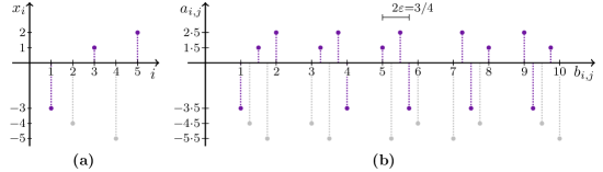
Figure 9: Illustrative example of the correspondence between zero-sum subsets and eliminability of approximately-merged units. (a) An affirmative Problem SSZ instance (cf. Figure 8) with collection ${x_{1},\ldots,x_{5}}=-3,-4,1,-5,2$ and zero-sum subset $S=\left\{1,3,5\right\}$ (observe $x_{1}+x_{3}+x_{5}=0$). (b) In unit group 3 of the constructed parameter, units $1$, $3$, and $4$ have outgoing weights $5\cdot x_{3}$, $5\cdot x_{5}$, and $5\cdot x_{1}$, respectively, and incoming weights within $2\varepsilon=\frac{3}{4}$. These units can be approximately merged and then the merged unit can be eliminated, since it has outgoing weight $5\cdot(x_{1}+x_{3}+x_{5})=0$.

($\texttt{PR-b}\in\mathcal{NP}$): Consider an instance $h,r\in{\mathbb{N}}$, $\varepsilon\in{{\mathbb{R}}^{+}}$, and $u=(a_{1},b_{1},\ldots,a_{h},b_{h})\in\mathcal{U}_{h}$. Use as a certificate a partition ${\Pi_{1},\ldots,\Pi_{J}}$ of ${\left\{\,i\in{\left\{{1},\ldots,{h}\right\}}\,:\,\operatorname{abs}(b_{i})>\varepsilon\,\right\}}$, such that (1) for each $\Pi_{j}$, for each $i,k\in\Pi_{j}$, $\operatorname{abs}(\operatorname{abs}(b_{i})-\operatorname{abs}(b_{k}))\leq 2\varepsilon$; and (2) at most $r$ of the $\Pi_{j}$ satisfy $\sum_{i\in\Pi_{j}}\operatorname{sign}(b_{i})\cdot a_{i}>\varepsilon\cdot{\left|\Pi_{j}\right|}$. The validity of such a certificate can be verified in polynomial time by checking each of these conditions directly. Such a certificate exists if and only if $\operatorname{prank}_{\varepsilon}(u)\leq r$, by similar reasoning as used in the proof of Theorem 6.2 ($\texttt{PR}\in\mathcal{NP}$).

Appendix H Hyperbolic tangent networks with multi-dimensional inputs and outputs

In the main paper we consider single-hidden-layer hyperbolic tangent networks with a single input unit and a single output unit. Our algorithms and results generalise to an architecture with multiple input units and multiple output units, with some minor changes.

Consider a family of fully-connected, feed-forward neural network architectures with $n\in{\mathbb{N}^{+}}$ input units, $m\in{\mathbb{N}^{+}}$ biased linear output units, and a single hidden layer of $h\in{\mathbb{N}}$ biased hidden units with the hyperbolic tangent nonlinearity. The weights and biases of the network are encoded in a parameter vector in the format $w=({{{a_{1},b_{1},c_{1}},\ldots,{a_{h},b_{h},c_{h}}}},d)\in\mathcal{W}^{n,m}_{h}={\mathbb{R}}^{(n+m+1)h+m}$, where for each hidden unit $i={{1},\ldots,{h}}$ there is an outgoing weight vector $a_{i}\in{\mathbb{R}}^{m}$, an incoming weight vector $b_{i}\in{\mathbb{R}}^{n}$, and a bias $c_{i}\in{\mathbb{R}}$; and $d\in{\mathbb{R}}^{m}$ is a vector of output unit biases. Thus each parameter $w\in\mathcal{W}^{n,m}_{h}$ indexes a function $f_{w}:{\mathbb{R}}^{n}\to{\mathbb{R}}^{m}$ such that $f_{w}(x)=d+\sum_{i=1}^{h}a_{i}\tanh(b_{i}\cdot x+c_{i})$.

The above notation is deliberately chosen to parallel the case $n=m=1$ considered in the main paper. This makes the generalisation of our results to the case $n,m\geq 1$ straightforward. First, replace all mentions of the scalar incoming and outgoing weights with incoming and outgoing weight vectors. It remains to note the following additional changes.

1. The algorithms and proofs commonly refer to the sign of an incoming weight. For $b\in{\mathbb{R}}^{n}$ define $\operatorname{sign}(b)\in\left\{-1,0,+1\right\}$ as the sign of the first nonzero component of $b$, or zero if $b=0$. Use this generalised sign function throughout when $n>1$.

2. Sorting the (signed) incoming weight and bias pairs of the hidden units is a key part of Algorithms 1 and 2. For pairs of the form $(b,c)\in{\mathbb{R}}^{n}\times{\mathbb{R}}$, lexicographically sort by the components of $b$ and then $c$.

3. The reducibility conditions were proven by Sussmann (1992) in the case $n\geq 1$ and $m=1$. The conditions also hold for $m\geq 1$ see Fukumizu, 1996; or Farrugia-Roberts, 2023, §A.

4. The construction of the centre of a bounding rectangle in the proof of Theorem 6.2 straightforwardly generalises to the construction of the centre of a bounding right cuboid.

For Theorem 6.2, the proof that $\texttt{UPC}\rightarrow\texttt{PR}$ requires no generalisation, because it suffices to construct instances of Problem PR with $n=m=1$. To see directly that Problem PR remains hard in networks with $n$ input units, compare with $\texttt{UVC}^{n+1}$ (Problem $\texttt{UVC}^{p}$ discussed in Appendix D; $n+1$ for $n$ incoming weights plus one bias for each hidden unit, see Appendix G for the biasless case).

References

- Albertini et al. (1993) Francesca Albertini, Eduardo D. Sontag, and Vincent Maillot. Uniqueness of weights for neural networks. In Artificial Neural Networks for Speech and Vision, pages 113–125. Chapman & Hall, London, 1993. Proceedings of a workshop held at Rutgers University in 1992. Access via Eduardo D. Sontag.
- Amari et al. (2006) Shun-ichi Amari, Hyeyoung Park, and Tomoko Ozeki. Singularities affect dynamics of learning in neuromanifolds. Neural Computation, 18(5):1007–1065, 2006. Access via Crossref.
- Amari et al. (2018) Shun-ichi Amari, Tomoko Ozeki, Ryo Karakida, Yuki Yoshida, and Masato Okada. Dynamics of learning in MLP: Natural gradient and singularity revisited. Neural Computation, 30(1):1–33, 2018. Access via Crossref.
- Aytekin et al. (2019) Caglar Aytekin, Francesco Cricri, and Emre Aksu. Compressibility loss for neural network weights. 2019. Preprint arXiv:1905.01044 [cs.LG].
- Berman et al. (2003) Piotr Berman, Alex D. Scott, and Marek Karpinski. Approximation hardness and satisfiability of bounded occurrence instances of SAT. Technical Report IHES/M/03/25, Institut des Hautes Études Scientifiques [Institute of Advanced Scientific Studies], 2003. Access via CERN.
- Buciluǎ et al. (2006) Cristian Buciluǎ, Rich Caruana, and Alexandru Niculescu-Mizil. Model compression. In Proceedings of the 12th ACM SIGKDD International Conference on Knowledge Discovery and Data Mining, pages 535–541. ACM, 2006. Access via Crossref.
- Casper et al. (2021) Stephen Casper, Xavier Boix, Vanessa D’Amario, Ling Guo, Martin Schrimpf, Kasper Vinken, and Gabriel Kreiman. Frivolous units: Wider networks are not really that wide. In Proceedings of the Thirty-Fifth AAAI Conference on Artificial Intelligence, volume 8, pages 6921–6929. AAAI Press, 2021. Access via Crossref.
- Cerioli et al. (2004) Márcia R. Cerioli, Luerbio Faria, Talita O. Ferreira, and Fábio Protti. On minimum clique partition and maximum independent set on unit disk graphs and penny graphs: Complexity and approximation. Electronic Notes in Discrete Mathematics, 18:73–79, 2004. Access via Crossref.
- Cerioli et al. (2011) Márcia R. Cerioli, Luerbio Faria, Talita O. Ferreira, and Fábio Protti. A note on maximum independent sets and minimum clique partitions in unit disk graphs and penny graphs: Complexity and approximation. RAIRO: Theoretical Informatics and Applications, 45(3):331–346, 2011. Access via Crossref.
- Chen et al. (1993) An Mei Chen, Haw-minn Lu, and Robert Hecht-Nielsen. On the geometry of feedforward neural network error surfaces. Neural Computation, 5(6):910–927, 1993. Access via Crossref.
- Cheng et al. (2018) Yu Cheng, Duo Wang, Pan Zhou, and Tao Zhang. Model compression and acceleration for deep neural networks: The principles, progress, and challenges. IEEE Signal Processing Magazine, 35(1):126–136, 2018. Access via Crossref.
- Cheng et al. (2020) Yu Cheng, Duo Wang, Pan Zhou, and Tao Zhang. A survey of model compression and acceleration for deep neural networks. 2020. Preprint arXiv:1710.09282v9 [cs.LG]. Updated version of Cheng et al. (2018).
- Choudhary et al. (2020) Tejalal Choudhary, Vipul Mishra, Anurag Goswami, and Jagannathan Sarangapani. A comprehensive survey on model compression and acceleration. Artificial Intelligence Review, 53(7):5113–5155, 2020. Access via Crossref.
- Clark et al. (1990) Brent N. Clark, Charles J. Colbourn, and David S. Johnson. Unit disk graphs. Discrete Mathematics, 86(1-3):165–177, 1990. Access via Crossref.
- Cook (1971) Stephen A. Cook. The complexity of theorem-proving procedures. In Proceedings of the Third Annual ACM Symposium on Theory of Computing, pages 151–158. ACM, 1971. Access via Crossref.
- Cousseau et al. (2008) Florent Cousseau, Tomoko Ozeki, and Shun-ichi Amari. Dynamics of learning in multilayer perceptrons near singularities. IEEE Transactions on Neural Networks, 19(8):1313–1328, 2008. Access via Crossref.
- Daniely et al. (2012) Amit Daniely, Nati Linial, and Michael Saks. Clustering is difficult only when it does not matter. 2012. Preprint arXiv:1205.4891 [cs.LG].
- Farrugia-Roberts (2022) Matthew Farrugia-Roberts. Structural Degeneracy in Neural Networks. Master’s thesis, School of Computing and Information Systems, The University of Melbourne, 2022. Access via Matthew Farrugia-Roberts.
- Farrugia-Roberts (2023) Matthew Farrugia-Roberts. Functional equivalence and path connectivity of reducible hyperbolic tangent networks. 2023. Preprint arXiv:2305.05089 [cs.NE].
- Fefferman (1994) Charles Fefferman. Reconstructing a neural net from its output. Revista Matemática Iberoamericana, 10(3):507–555, 1994. Access via Crossref.
- Fefferman and Markel (1993) Charles Fefferman and Scott Markel. Recovering a feed-forward net from its output. In Advances in Neural Information Processing Systems 6, pages 335–342. Morgan Kaufmann, 1993. Access via NeurIPS.
- Fukumizu (1996) Kenji Fukumizu. A regularity condition of the information matrix of a multilayer perceptron network. Neural Networks, 9(5):871–879, 1996. Access via Crossref.
- Fukumizu and Amari (2000) Kenji Fukumizu and Shun-ichi Amari. Local minima and plateaus in hierarchical structures of multilayer perceptrons. Neural Networks, 13(3):317–327, 2000. Access via Crossref.
- Fukumizu et al. (2019) Kenji Fukumizu, Shoichiro Yamaguchi, Yoh-ichi Mototake, and Mirai Tanaka. Semi-flat minima and saddle points by embedding neural networks to overparameterization. In Advances in Neural Information Processing Systems 32, pages 13868–13876. Curran Associates, 2019. Access via NeurIPS.
- Garey and Johnson (1979) Michael R. Garey and David S. Johnson. Computers and Intractability: A Guide to the Theory of NP-Completeness. W. H. Freeman and Company, 1979.
- Hakimi (1964) S. L. Hakimi. Optimum locations of switching centers and the absolute centers and medians of a graph. Operations Research, 12(3):450–459, 1964. Access via Crossref.
- Hakimi (1965) S. L. Hakimi. Optimum distribution of switching centers in a communication network and some related graph theoretic problems. Operations Research, 13(3):462–475, 1965. Access via Crossref.
- Hinton and van Camp (1993) Geoffrey E. Hinton and Drew van Camp. Keeping the neural networks simple by minimizing the description length of the weights. In Proceedings of the Sixth Annual Conference on Computational Learning Theory, pages 5–13. ACM, 1993. Access via Crossref.
- Hinton et al. (2014) Geoffrey E. Hinton, Oriol Vinyals, and Jeff Dean. Distilling the knowledge in a neural network. Presented at Twenty-eighth Conference on Neural Information Processing Systems, Deep Learning workshop, 2014. Preprint arXiv:1503.02531 [stat.ML].
- Jansen and Müller (1995) Klaus Jansen and Haiko Müller. The minimum broadcast time problem for several processor networks. Theoretical Computer Science, 147(1-2):69–85, 1995. Access via Crossref.
- Kariv and Hakimi (1979) O. Kariv and S. L. Hakimi. An algorithmic approach to network location problems. I: the -centers. SIAM Journal on Applied Mathematics, 37(3):513–538, 1979. Access via Crossref.
- Karp (1972) Richard M. Karp. Reducibility among combinatorial problems. In Complexity of Computer Computations, pages 85–103. Springer, 1972. Access via Crossref.
- Kůrková and Kainen (1994) Věra Kůrková and Paul C. Kainen. Functionally equivalent feedforward neural networks. Neural Computation, 6(3):543–558, 1994. Access via Crossref.
- Levin (1973) Leonid A. Levin. Universal sequential search problems. Problemy Peredachi Informatsii [Problems of Information Transmission], 9(3):115–116, 1973. In Russian. Translated into English in Trakhtenbrot (1984).
- Lichtenstein (1982) David Lichtenstein. Planar formulae and their uses. SIAM Journal on Computing, 11(2):329–343, 1982. Access via Crossref.
- Liu et al. (1998) Yanpei Liu, Aurora Morgana, and Bruno Simeone. A linear algorithm for 2-bend embeddings of planar graphs in the two-dimensional grid. Discrete Applied Mathematics, 81(1-3):69–91, 1998. Access via Crossref.
- Mahajan et al. (2012) Meena Mahajan, Prajakta Nimbhorkar, and Kasturi Varadarajan. The planar -means problem is NP-hard. Theoretical Computer Science, 442:13–21, 2012. Access via Crossref.
- Megiddo and Supowit (1984) Nimrod Megiddo and Kenneth J. Supowit. On the complexity of some common geometric location problems. SIAM Journal on Computing, 13(1):182–196, 1984. Access via Crossref.
- Phuong and Lampert (2020) Mary Phuong and Christoph H. Lampert. Functional vs. parametric equivalence of ReLU networks. In 8th International Conference on Learning Representations. OpenReview, 2020. Access via OpenReview.
- Piziak and Odell (1999) R. Piziak and P. L. Odell. Full rank factorization of matrices. Mathematics Magazine, 72(3):193–201, 1999. Access via Crossref.
- Sanh et al. (2019) Victor Sanh, Lysandre Debut, Julien Chaumond, and Thomas Wolf. DistilBERT, a distilled version of BERT: Smaller, faster, cheaper and lighter. Presented at the Fifth Workshop on Energy Efficient Machine Learning and Cognitive Computing, 2019. Preprint arXiv:1910.01108 [cs.CL].
- Şimşek et al. (2021) Berfin Şimşek, François Ged, Arthur Jacot, Francesco Spadaro, Clément Hongler, Wulfram Gerstner, and Johanni Brea. Geometry of the loss landscape in overparameterized neural networks: Symmetries and invariances. In Proceedings of the 38th International Conference on Machine Learning, pages 9722–9732. PMLR, 2021. Access via PMLR.
- Supowit (1981) Kenneth J. Supowit. Topics in Computational Geometry. Ph.D. thesis, University of Illinois at Urbana-Champaign, 1981. Access via ProQuest.
- Sussmann (1992) Héctor J. Sussmann. Uniqueness of the weights for minimal feedforward nets with a given input-output map. Neural Networks, 5(4):589–593, 1992. Access via Crossref.
- Suzuki et al. (2020a) Taiji Suzuki, Hiroshi Abe, Tomoya Murata, Shingo Horiuchi, Kotaro Ito, Tokuma Wachi, So Hirai, Masatoshi Yukishima, and Tomoaki Nishimura. Spectral pruning: Compressing deep neural networks via spectral analysis and its generalization error. In Proceedings of the Twenty-Ninth International Joint Conference on Artificial Intelligence, pages 2839–2846. IJCAI, 2020a. Access via Crossref.
- Suzuki et al. (2020b) Taiji Suzuki, Hiroshi Abe, and Tomoaki Nishimura. Compression based bound for non-compressed network: Unified generalization error analysis of large compressible deep neural network. In 8th International Conference on Learning Representations. OpenReview, 2020b. Access via OpenReview.
- Tovey (1984) Craig A. Tovey. A simplified NP-complete satisfiability problem. Discrete Applied Mathematics, 8(1):85–89, 1984. Access via Crossref.
- Trakhtenbrot (1984) Boris A. Trakhtenbrot. A survey of Russian approaches to perebor (brute-force search) algorithms. Annals of the History of Computing, 6(4):384–400, 1984. Access via Crossref.
- Valiant (1981) Leslie G. Valiant. Universality considerations in VLSI circuits. IEEE Transactions on Computers, 100(2):135–140, 1981. Access via Crossref.
- Vlačić and Bölcskei (2021) Verner Vlačić and Helmut Bölcskei. Affine symmetries and neural network identifiability. Advances in Mathematics, 376:107485, 2021. Access via Crossref.
- Vlačić and Bölcskei (2022) Verner Vlačić and Helmut Bölcskei. Neural network identifiability for a family of sigmoidal nonlinearities. Constructive Approximation, 55(1):173–224, 2022. Access via Crossref.
- Watanabe (2009) Sumio Watanabe. Algebraic Geometry and Statistical Learning Theory. Cambridge University Press, 2009.
- Wei et al. (2008) Haikun Wei, Jun Zhang, Florent Cousseau, Tomoko Ozeki, and Shun-ichi Amari. Dynamics of learning near singularities in layered networks. Neural Computation, 20(3):813–843, 2008. Access via Crossref.
- Wei et al. (2022) Susan Wei, Daniel Murfet, Mingming Gong, Hui Li, Jesse Gell-Redman, and Thomas Quella. Deep learning is singular, and that’s good. IEEE Transactions on Neural Networks and Learning Systems, 2022. Access via Crossref. To appear in an upcoming volume.
- Zhang et al. (2017) Chiyuan Zhang, Samy Bengio, Moritz Hardt, Benjamin Recht, and Oriol Vinyals. Understanding deep learning requires rethinking generalization. In 5th International Conference on Learning Representations. OpenReview, 2017. Access via OpenReview.
- Zhang et al. (2021) Chiyuan Zhang, Samy Bengio, Moritz Hardt, Benjamin Recht, and Oriol Vinyals. Understanding deep learning (still) requires rethinking generalization. Communications of the ACM, 64(3):107–115, 2021. Access via Crossref. Republication of Zhang et al. (2017).