Probabilistic Region-of-Attraction Estimation with Scenario Optimization and Converse Theorems

Abstract

The region of attraction characterizes well-behaved and safe operation of a nonlinear system and is hence sought after for verification. In this paper, a framework for probabilistic region of attraction estimation is developed that combines scenario optimization and converse theorems. With this approach, the probability of an unstable condition being included in the estimate is independent of the system’s complexity, while convergence in probability to the true region of attraction is proven. Numerical examples demonstrate the effectiveness for optimization-based control applications. Combining systems theory and sampling, the complexity of Monte–Carlo-based verification techniques can be reduced. The results can be extended to arbitrary level sets of which the defining function can be sampled, such as finite-horizon viability. Thus, the proposed approach is applicable and/or adaptable to verification of a wide range of safety-related properties for nonlinear systems including feedback laws based on optimization or learning.

I Introduction

Estimating the region of attraction is a classical problem in the analysis of nonlinear dynamic systems [1]. The region of attraction of a dynamic system is the set of all initial conditions such that system states asymptotically converge to a given equilibrium, thus describing admissible excitations. For closed-loop nonlinear control systems, the region of attraction is typically bounded due to inaccuracies of the underlying models or physical limitations of the controls. By assessing that the region of attraction is sufficiently large, stable asymptotic behaviour of a nonlinear system can be verified for the envisaged operating envelope. Recently, region-of-attraction estimation has seen increased interest in the context of feasibility of model-predictive control [2, 3], stability of time-distributed optimization [4], and verification of neural networks [5, 6, 7]. For the purpose of verification, the region-of-attraction estimate should be nonconservative without overapproximating the true set.

The estimation is often cast as the problem to find a Lyapunov functions subject to a dissipation inequality but analytical solutions (such as sum-of-squares optimization [5, 6, 7, 8, 9, 10]) often require an algebraic (polynomial) approximation of the system dynamics. Furthermore, the complexity of sum-of-squares problems notoriously increases with the number of states considered, a particular issue for methods based on optimization and machine learning with numerous controller states. An alternative are data-driven methods exploiting converse Lyapunov theorems [11, 12], which approximate a Lyapunov function based on sampled, stable trajectories. These approaches face some major challgenges: First, judging asymptotic behaviour from finite sequences involves guess work; and second, there are no guarantees for the approximation to be a subset of the true region of attraction. Relaxing asymptotic convergence to finite-step reachability of a provably stable subset, scenario optimization can provide probabilistic bounds for the accuracy of the region-of-attraction estimate based on the number of samples [13]. Previous work on data-driven reachable set estimation considered probabilistic outer approximations by ellipsoids [14]. For the complementary problem of maximal positively invariant set, [15] proved probabilistic bounds for sample-based estimates using arbitrary basis functions; however, the number of samples to ensure a given confidence level is difficult to compute and grows exponentially with the dimension of the basis. In [16], subsets of the region of attraction were approximated by spheres or polyhedra which only provide conservative estimates.

In this paper, we focus on estimating the region of attraction for a class of linear systems commonly arising in optimization schemes and neural networks. We employ a limit on the truncated converse Lyapunov function given by [17] as sufficient condition for asymptotic stability of a finitely sampled sequence; for the class of systems in this paper, we can find an upper bound as maximum of a monotone scalar function. Solving optimization problems over two independent sets of sampled stable and unstable trajectories, respectively, we aim to find a probabilistic (inner) approximations with a polynomial shape obtained from data. We prove that our approximations converge (in probability and distance) to the true region of attraction if the number of samples and the maximum polynomial degree increases. Parts of our results can, with minor modifications, also be used for the approximation of reachable sets and/or applied to general, nonlinear or even unknown dynamics.

The remainder of this paper is organized as follows: Section II states the problem of region of attraction estimation via truncated converse Lyapunov functions. Section III-B defines optimization over random variables and relates the sample complexity to the reliability of the empirical maximum; Section III-C introduces the notion of inner and outer approximations for the region of attraction; Section IV-A presents our main probabilistic algorithm. The algorithm is analyzed and its convergence in probability to the true region of attraction is proven in Section V. Finally, numerical examples for saturated LQR and suboptimal model-predictive control are presented in Section VI.

Notation

Let $\mathbb{N}$ and $\mathbb{R}$ denote the natural and real numbers, respectively. We consider the Euclidean space $\mathbb{R}^{n}$ equipped with inner product $\langle\cdot,\cdot\rangle:\mathbb{R}^{n}\times\mathbb{R}^{n}\to\mathbb{R}$ and induced norm $\|\cdot\|_{2}:x\mapsto\sqrt{\langle x,x\rangle}$. Let $\mathbb{S}_{m}$ (resp., $\mathbb{S}_{m}^{+}$) denote the subset of symmetric (resp., positive semidefinite) matrices in $\mathbb{R}^{m\times m}$ and take $A,B\in\mathbb{R}^{m\times\ell}$; the Frobenius inner product is $\langle A,B\rangle=\operatorname{trace}(A^{\mathrm{T}}B)$; and the Kronecker outer product is $A\otimes B\in\mathbb{R}^{m\ell\times m\ell}$. The norm ball of radius $r>0$, excluding the origin, is defined as $\mathscr{B}^{*}(r)=\{x\in\mathbb{R}^{n}\mid 0<\|x\|_{2}<r\}$. When applied to vectors of same lengths, the inequalities “$\leq$” and “$\geq$” are to be understood element-wise.

A probability space is a tuple $(\Omega,\Sigma,P)$, where $\Omega$ is the sample space, the events $\Sigma$ are a $\sigma$-algebra of subsets of $\Omega$, and the probability function $P:\Sigma\to[0,1]$ satisfies that $P(\Omega)=1$ and $P(S_{1}\cup S_{2})=P(S_{1})+P(S_{2})$ for any $S_{1},S_{2}\subset\Omega$ with $S_{1}\cap S_{2}=\varnothing$. A random variable defined on a probability space $(\Omega,\Sigma,P)$ is a measurable function $z:\Omega\to\mathcal{S}$, or $z\in\mathcal{S}^{\Omega}$ for short, where $\mathcal{S}$ is a finite-dimensional vector space (the support of $z$); we write the probability that $z\in A$ for some $A\subset\mathcal{S}$ as $\operatorname{P}\{z\in A\}=P(\{\omega\in\Omega\,|\,z(\omega)\in A\})$. A sequence of random variables $\{z_{k}\in\Omega\to\mathcal{S}\}_{k\geq 0}$, or short $\{z_{k}\}_{k\geq 0}\subset\mathcal{S}^{\Omega}$, is said to converge almost surely to the random variable $z\in\mathcal{S}^{\Omega}$ if and only if

$$\operatorname{P}\{\lim_{k\to\infty}\|z_{k}-z\|_{2}=0\}=1$$

and to converge in probability to $z$ if and only if

$$\lim_{k\to\infty}\operatorname{P}\{\|z_{k}-z\|_{2}<\epsilon\}=1$$

for any $\epsilon>0$.

We denote the vector of monomials of $y\in\mathbb{R}^{n}$ up to degree $q\in\mathbb{N}$ by $Z_{q}\{y\}$, its length by $n_{q}$, and the outer product as $Z_{q}^{2}=Z_{q}\otimes Z_{q}$. A polynomial function $p:\mathcal{D}\to\mathbb{R}$ with coefficients $\theta\in\mathbb{R}^{n_{q}}$ is given by $p:y\mapsto\langle\theta,Z_{q}\{y\}\rangle$.

II Problem Statement

We consider solutions $\{x_{k}\}_{k\geq 0}\subset\mathbb{R}^{n}$ to the discrete-time initial value problem

$$\Pi(x):\,\left\{\begin{aligned} x_{k+1}&=Ax_{k}+\phi(x_{k})\\ x_{0}&=x\end{aligned}\right.$$ (1)

where $\mathbb{R}^{n}$ is the state space, $A:\mathbb{R}^{n}\to\mathbb{R}^{n}$ is a linear operator, and $\phi:\mathbb{R}^{n}\to\mathbb{R}^{n}$ is a deterministic nonlinear operator. The dynamics $\Pi(x)$ are possibly unknown but bestowed with the following assumption.

Assumption 1

The function $\phi$ is Lipschitz continuous and satisfies $\phi(0)=0$. Moreover, the origin is locally asymptotically stable for (1).

Since we assume that (1) is locally asymptotically stable around the origin, trajectories starting sufficiently close to the origin remain close and there exists a nonempty (but not necessarily connected) set of initial conditions that lead to converging state trajectories.

Definition 1

The true region of attraction $\mathcal{R}_{\infty}$ of (1) is the largest set $R\subset\mathbb{R}^{n}$ such that any solution $\{x_{k}\}_{k\geq 0}$ of $\Pi(x)$ converges to the origin if $x\in R$.

We introduce the Hausdorff distance of two bounded sets $A,B\subset\mathbb{R}^{n}$ as

$$\varrho_{\mathrm{H}}(A,B)=\max\{\sup_{x\in A}\operatorname{dist}(x;B),\sup_{y\in B}\operatorname{dist}(y;A)\}$$

where $\operatorname{dist}$ denotes the distance between a point and a set, i.e., $\operatorname{dist}(x;B)=\inf_{y\in B}\|x-y\|_{2}$.

Problem 1

Solve

$$\min_{\theta}\varrho_{\mathrm{H}}(R_{\theta},\mathcal{R}_{\infty})\quad\text{s.t. $R_{\theta}\subset\mathcal{R}_{\infty}$}$$

where $R_{\theta}\subset\mathbb{R}^{n}$ is a set estimate parametrized by $\theta$.

By Assumption 1, the origin is a stationary condition and $\phi$ is bound (by $\zeta>0$), that is, $||\phi(x)||\leq\zeta||x||$ holds for all $x\in\mathbb{R}^{n}$. Such systems arise in control of linear systems by neural networks, where the state space comprises of system states and hidden layer neurons, and $\phi$ is a nonlinear activation function (such as $\tanh$ or $\max\{x,0\}$); in linear model-predictive control using a convex solver, possibly with a fixed number of iterations, where $\phi$ is the projection onto the feasible set; or, with some relaxation of the continuity assumptions, in the analysis of transitional flows for nonlinear fluids [18]. The state space typically is an Euclidean vector space.

In this paper, we rely on data to compute $\theta$. We assume that we can sample the solution of $\Pi(x)$ for any (finite) set of initial conditions $x\in\mathbb{R}^{n}$ of our choice and observe a finite-horizon response $\{x_{k}\}_{k=0}^{p}$ with $p\in\mathbb{N}$. This approach raises a number of challenges: To begin with, we cannot decide beyond doubt whether the solution is going to converge to the origin, that is, whether $x\in\mathcal{R}_{\infty}$. Instead, we are going to introduce a family of finite-time decidable sets $\mathcal{R}_{p}\subset\mathcal{R}_{\infty}$ approaching $\mathcal{R}_{p}$ as $p\to\infty$ and compute an estimate for $\mathcal{R}_{p}$ for some given $p$. Reliance on finite data samples also means that we cannot guarantee that our estimate $R_{\theta}$ is a true subset of $\mathcal{R}_{p}$. We will hence resort to a notion of probabilistic set approximation that allows us to bound the probability that a point is incorrectly predicted to be stable. At last, we need to carefully choose a parametrization that allows us to approximate $\mathcal{R}_{p}$ arbitrarily well. To that extent, we will associate $R_{\theta}$ as the sublevel set of a polynomial function $v$ and $\theta$ with its vector of coefficients.

Objectives

Let $p\in\mathbb{N}$ be given. The goal of this paper is to obtain an estimate $R_{\theta}$ of $\mathcal{R}_{p}$, parametrized by the vector of polynomial coefficients $\theta$, based on sample trajectories of (1) subject to the following probabilistic objectives.

1. Accuracy: The probability that a point $x\in R_{\theta}$ is not in $\mathcal{R}_{p}$ is bounded by some $\epsilon>0$.

2. Validity: The bound $\epsilon$ is given specifically and independently of the polynomial degree.

3. Convergence: With increasing polynomial degree, the estimates $R$ approaches.

Such estimates of the region of attraction can be used as certificates for correct behaviour of a nonlinear system.

Related work

The problem of estimating $\mathcal{R}_{\infty}$ for a given system has a long history in nonlinear analysis. A popular choice are approaches based on polynomial Lyapunov functions. Polynomial approximation for $\mathcal{R}_{\infty}$ aims to find a sublevel set

$$R_{v,c}=\{x\in\mathbb{R}^{n}\mid v(x)\leq c\}$$

where $v:\mathbb{R}^{n}\to\mathbb{R}$ is a polynomial function and $c\geq 0$, that

• minimizes $\varrho_{\mathrm{H}}(R_{v,c},\mathcal{R}_{\infty}$; and

• ensures that $R$ is a subset of $\mathcal{R}_{\infty}$.

Methods to approximate the region of attraction by constrained polynomial optimisation include [8, 19]. A more tractable relaxation is to obtain the shape $v(\cdot)$ by unconstrained optimization, then search for the largest level set that is contained by $R_{\infty}$. This is the strategy employed in [20]. The works cited here rely on dissipativity conditions to provide sufficient conditions for a Lyapunov function and are computationally heavy.

III Mathematical Background

A candidate Lyapunov function is the partial sum

$$V_{p}(x)=_{\text{def}}\sum_{k=0}^{p}\|x_{k}\|_{2}^{2}$$ (2)

where $\{x_{k}\}_{k\geq 0}\subset\mathbb{R}^{n}$ solves $\Pi(x)$ and $p\in\mathbb{N}\cup\{\infty\}$. It is easy to see that, if converging, $V_{\infty}$ is a Lyapunov function and thus, its domain is a subset of $\mathcal{R}_{\infty}$. Reverse statements, that is, conditions under which the domain of $V_{\infty}$ equals the (true) region of attraction of (1), are known as converse theorems [21, 22, 23, 24]. In general, the region of attraction is undecidable [25] and hence, there exists no computational form of $V_{\infty}$.

III-A Truncated Lyapunov function

We rely on the results of [17] for a lower bound on the truncated series. Choose $\tilde{p}\in\mathbb{N}$ and $\tilde{r}>0$ such that any trajectory $\{x_{k}\}_{k\geq 0}$ with $x_{0}\in\mathscr{B}^{*}(\tilde{r})$ satisfies

$$\|x_{p}\|_{2}<\|x_{0}\|_{2}$$

for all $p\in\{\tilde{p},\tilde{p}+1,\ldots,2\tilde{p}-1\}$. It can then be shown that any trajectory $\{x_{k}\}_{k\geq 0}$ with $x_{0}\in\mathscr{B}^{*}(\tilde{r})$ satisfies $x_{k}\in\mathscr{B}^{*}(\tilde{r})$ for all $k\geq\tilde{p}$. In order to efficiently decide $\mathcal{R}_{p}$, we compute a lower bound for $\bar{r}$ in the appendix. For any $p\geq\tilde{p}$, we define

$$\mathcal{R}_{p}=\{x\in\mathbb{R}^{n}\mid V_{p}(x)<c_{p}\}$$ (3)

where $c_{p}=(p+1)\tilde{r}^{2}$. We obtain the following result.

Theorem 1

Let $x\in\mathbb{R}^{n}$ be an initial condition for (1); $x\in\mathcal{R}_{\infty}$ if and only if there exists $p\geq\tilde{p}$ such that $x\in\mathcal{R}_{p}$.

Proof:

See [17, Theorems 3.7 and 3.10]. ∎

In other words, when sampling the solution of $\Pi(x)$ for some given $x\in\mathbb{R}^{n}$, we can decide whether or not $x\in\mathcal{R}_{p}$ after a finite number of steps. Given $p\geq\tilde{p}$, the polynomial approximation problem of $\mathcal{R}_{p}$ can be written as

$$\min_{v(\cdot)}\sup_{x\in\mathcal{R}_{p}}\|v(x)-V_{p}(x)\|_{2}\quad\text{s.t. $R\subseteq\mathcal{R}_{p}$}$$ (4)

where $v$ is a polynomial function with real-valued coefficients and fixed degree.

III-B Scenario Optimization

When using data to solve optimization problems such as (4), deterministic constraints are replaced by so-called chance constraints leading to a probabilistic optimization. The scenario approach of [13] then links the sample complexity of the randomized algorithm to its reliability and accuracy with respect to the original, deterministic optimization problem.

Definition 2

Let $z\in\mathcal{S}^{\Omega}$ be a random variable, $\Theta\in\mathbb{R}^{n_{\Theta}}$ be a set of parameter vectors, and $f:\mathcal{S}\to\mathbb{R}$ be a measurable cost function; the probabilistic supremum $\sup^{\epsilon}f(z)$ for $\epsilon>0$ is the smallest number $\gamma$ satisfying $\operatorname{P}\{f(z)\leq\gamma\}\geq 1-\epsilon$. Moreover, the empirical maximum is given as

$$\max^{N}f(z)=\max_{i\in\{1,\ldots,N\}}f(z^{(i)})$$ (5)

where $(z^{(1)},\ldots,z^{(N)})\subset\mathcal{S}^{\Omega}$ is a tuple of $N\in\mathbb{N}$ independent random variables (the samples) with distribution identical to that of $z$.

It can be shown [13, Theorem 7.4] that $\max^{N}f(z)$ converges almost surely to $\sup f(z)$ if $N\to\infty$, provided that $f$ is continuous at the optimal solution $\hat{z}$ of $\sup f(z)$ and $\operatorname{P}\{z\in B\}>0$ for any neighbourhood $B\subset\mathcal{S}$ of $\hat{z}$.

When estimating the region of attraction using trajectory samples, we are going to optimize over the empirical maximum of a parametrized cost function. To study accuracy and convergence of our result, we define the probabilistic optimization problems

$$\hat{\gamma} =\min_{\beta}\sup_{z}g(\beta,z)$$ (6a)

$$\gamma_{\epsilon} =\min_{\beta}\sup_{z}^{\epsilon}g(\beta,z)$$ (6b)

$$\gamma^{N} =\min_{\beta}\max_{z}^{N}g(\beta,z)$$ (6c)

where $\beta\in\Theta$ and $g:\mathcal{S}\times\Theta\to\mathbb{R}$ is measurable. If either $\Theta$ is compact or $g$ is bounded from below, then $\gamma^{N}$ is a well-defined random variable with support in $(-\infty,\hat{\gamma}]$. Here, (6c) represents the optimization problem our randomized algorithm will solve; Eq. (6a) corresponds to the original problem; and (6b) is used to formulate the following, probabilistic results. Denote the optimal solution(s) to (6) by $\arg\hat{\gamma}$, $\arg\gamma_{\epsilon}$, and $\arg\gamma^{N}$, respectively.

Lemma 1

Let $\epsilon,\delta>0$ be confidence levels; then there exists $N\in\mathbb{N}$ such that

$$\operatorname{P}\{\gamma^{N}<\gamma_{\epsilon}\}<\delta$$ (7)

In addition, let $\Theta$ be compact and convex, $g(\beta,\cdot)$ be convex in $\beta$, and $\beta_{N}\in\arg\gamma^{N}$ be unique; if

$$\epsilon\,N\geq\frac{e}{e-1}(\log\delta^{-1}+n_{\Theta})$$ (8)

where $\log(\cdot)$ denotes the natural logarithm and $e$ its base, then $\operatorname{P}\{\gamma^{N}<\sup_{z}^{\epsilon}g(\beta_{N},z)\}<\delta$.

Proof:

See [13, Theorem 8.1 and Corollary 12.1] as well as remarks. ∎

In other words, the scenario optimization (6c) is $\delta$-reliable in the sense that with probability $1-\delta$ or greater, its optimal solution is $\epsilon$-accurate, that is, $\gamma^{N}$ is an upper bound of $g(\beta_{N},z)$ for $z\in\mathcal{S}^{\Omega}$ with probability of at least $1-\epsilon$. The number of samples $N$ that is necessary to satisfy the confidence levels $\epsilon$ and $\delta$ is called sample complexity. We will apply scenario optimization to polynomial regression. Here, $\Theta$ will denote the space of coefficient vectors (up to given degree) and the cost function is linear in the coefficients.

Optimization in multiple variables

We can extend (6) to optimization problems with multiple random variables, viz.

$$\gamma^{\prime}=\min_{\beta}\sup_{z_{1},z_{2}}\max\{g_{1}(\beta,z_{1}),g_{2}(\beta,z_{2})\}$$ (9)

where $z_{1}\in\mathcal{S}_{1}^{\Omega}$ and $z_{2}\in\mathcal{S}_{2}^{\Omega}$ are random variables and $g_{1,2}:\Theta\times\mathcal{S}_{1,2}\to\mathbb{R}$ are measurable functions that are convex in the first variable. It is easy to see that (9) is equivalent to the optimization problem in (6a) for the extended cost function

$$\bar{g}:(\beta,z)\mapsto\max\{g_{1}(\beta,z_{1}),g_{2}(\beta,z_{2})\}$$

with $z=(z_{1},z_{2})$, which is again convex in $\beta$. Let again $\gamma_{\epsilon}$ and $\gamma^{N}$ denote the optimal values of the probabilistic optimization problems (6b) and (6c), respectively, for $\bar{g}$. We obtain the following strengthening of Lemma 1.

Proposition 1

Let $\epsilon,\delta>0$ be confidence levels, let $\Omega$ be compact and convex, and $\beta_{N}\in\arg\gamma^{N}$ be unique; then

$$\operatorname{P}\{\gamma^{N}<\sup_{z_{i}}^{\epsilon}g_{i}(\beta_{N},z_{i})\}<\delta$$

for $i\in\{1,2\}$ if (8) is satisfied by $\epsilon$ and $\delta$.

Proof:

For any $\gamma\in\mathbb{R}$ and $\beta\in\Theta$, we have that $\bar{g}(\beta,z)\leq\gamma$ if and only if $g_{1}(\beta,z_{1})\leq\gamma$ and $g_{2}(\beta,z_{2})\leq\gamma$; that is,

$$\operatorname{P}\{\bar{g}(\beta,z)\leq\gamma\} \leq\operatorname{P}\{g_{i}(\beta,z_{i})\leq\gamma\}$$

and hence, $\sup_{z_{i}}^{\epsilon}g_{i}(\beta,z_{i})\leq\sup_{z}^{\epsilon}\bar{g}(\beta,z)$ for $i\in\{1,2\}$. The desired result then follows from Lemma 1. ∎

III-C Polynomial Set Approximations

We want to establish polynomial estimates of $\mathcal{R}_{p}$ by scenario optimization. As data-driven approaches rarely yield estimates that are guaranteed to be inner or outer approximations, we introduce a probabilistic equivalent. We consider a subset $\mathcal{X}\subset\mathbb{R}^{n}$ of the state space.

Definition 3

Take $\epsilon>0$ and let $x\in\mathcal{X}^{\Omega}$ be a random variable; a set $X\subset\mathbb{R}^{n}$ is an $\epsilon$-accurate outer approximation of $\mathcal{X}$ if and only if $\operatorname{P}\{x\in X\}\geq 1-\epsilon$.

Intuitively, the probability that $x\in\mathcal{X}^{\Omega}$ is not in $X$ is less than $\epsilon$. We define a probabilistic inner approximation likewise.

Definition 4

Take $\epsilon>0$ and let $x\in(\mathbb{R}^{n}\setminus\mathcal{X})^{\Omega}$ be a random variable; a set $X\subset\mathbb{R}^{n}$ is an $\epsilon$-accurate inner approximation of $\mathcal{X}$ if and only if $\operatorname{P}\{x\not\in X\}\geq 1-\epsilon$.

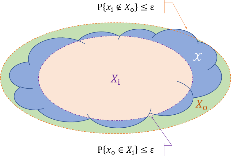
Figure 1: Illustration of $\epsilon$-accurate inner and outer approximations $X_{\mathrm{i}}$ and $X_{\mathrm{o}}$ of some set $\mathcal{X}$ with random variables $x_{\mathrm{i}}\in\mathcal{X}$ and $x_{\mathrm{o}}\in\mathbb{R}^{n}\setminus\mathcal{X}$.

The concept of probabilistic inner and outer approximates is illustrated in Fig. 1. Indeed, any sufficiently small (or large) set is likely to be an inner (outer) approximation. Therefore, we aim to find the probabilistic inner approximation which is, at the same time, as close as possible to an accurate outer approximation. As demonstrated in the following result, the notion of set approximations is tied to that of scenario optimization.

Proposition 2

Let $z\in\mathcal{X}^{\Omega}$ be a random variable, $f:\mathbb{R}^{n}\to\mathbb{R}$ be a measurable function, and $\epsilon,\delta>0$ be confidence levels; then there exists $N\in\mathbb{N}$ such that

$$X_{N}=\{x\in\mathbb{R}^{n}\,|\,f(x)\leq\max^{N}f(z)\}$$

is an $\epsilon$-accurate outer approximation of $\mathcal{X}$ with probability $1-\delta$ or larger.

Proof:

Define $\gamma^{N}=\max^{N}f(z)$; by virtue of Lemma 1, there exists $N\in\mathbb{N}$ such that $\operatorname{P}\{\gamma_{\epsilon}\leq\gamma^{N}\}\geq 1-\delta$ and $\operatorname{P}\{f(z)\leq\gamma_{\epsilon}\}\geq 1-\epsilon$, where $\gamma_{\epsilon}=\sup^{\epsilon}f(z)$ is the probabilistic supremum of $f$ on $z\in\mathcal{X}$. Hence,

$$\operatorname{P}\{\operatorname{P}\{f(z)\leq\gamma^{N}\}\geq 1-\epsilon\}\geq 1-\delta$$

which is the desired result by definition of $X_{N}$. ∎

It is not hard to derive a similar result for the inner approximation of $\mathcal{X}$; moreover, an explicit bound for $N$ based on $\epsilon$ and $\delta$ is obtained from (8) with $n_{\beta}=0$. In Proposition 2, a probabilistic outer approximation of $\mathcal{X}$ is given as sublevel set $X_{N}$ of a function $f$ of which the level is determined by sampling $f$ on $\mathcal{X}$. The probability of a point $x\in\mathcal{X}$ not being in the sublevel set thus is equal to the probability of the empirical maximum being smaller than $f(x)$. Hence, accuracy of $X_{N}$ is linked to scenario optimization.

Clearly, an arbitrary choice for the function $f(\cdot)$ is likely not to lead to a good approximation. The work of [14] searched for the smallest ellipsoidal set that is an accurate outer approximation of $\mathcal{X}$ without any statement for inner approximations. Unfortunately, this approach cannot be easily applied to inner approximations as the empirical maximum of the volume is unbounded. Instead, we are going to use polynomial functions and compute the vector of coefficients as randomized algorithm. For the analysis, we apply to the result of Stone and Weierstrass. Here, let $f:\mathcal{D}\to\mathbb{R}$ be a given scalar function on $\mathcal{D}\subset\mathbb{R}^{n}$.

Lemma 2

Let $\eta>0$; if $f$ is Lipschitz continuous and $\mathcal{D}$ is compact, then there exists $q\in\mathbb{N}$ such that

$$\sup_{y\in\mathcal{D}}|\langle\theta,Z_{q}\{y\}\rangle-f(y)|\leq\eta$$

for some vector $\theta\in\mathbb{R}^{n_{q}}$.

Proof:

By [26, Chapter 20, Theorem 3], the polynomials in $y$ form a dense subset of the continuous functions on $\mathcal{D}$, that is, there exists a sequence of polynomials $\{p:\mathcal{D}\to\mathbb{R}\}$ that converges uniformly to $f$. Take $q$ as the degree of $\hat{p}$ such that $\sup_{y\in\mathcal{D}}|\hat{p}(y)-f(y)|\leq\eta$ to complete the proof. ∎

IV Methodology

We will present a relaxed solution to the polynomial approximation problem of which the accuracy of the inner approximation is independent of either the polynomial degree or the number of system states. Our approach is based on obtaining a probabilistic polynomial approximation for $V_{p}$ on $\mathcal{R}_{p}$, while guaranteeing that the resulting estimate is a probabilistic inner approximation. For that purpose, we solve two empirical optimization problems as summarized in Alg. 1; the first problem is to obtain a polynomial approximation of $V_{p}$ and the second problem is to correct for initial conditions outside of $\mathcal{R}_{p}$ lying inside the polynomial sublevel set of level $c_{p}$.

As we are going to show, the result of the probabilistic algorithm is accurate and reliable in the sense that the region of attraction estimate is an $\epsilon$-accurate inner approximation of $\mathcal{R}_{p}$ with probability $1-\delta$ or larger, where the confidence levels $(\epsilon,\delta)$ depend on the number of samples but not the degree of the polynomial approximation. In addition, in the next section, we prove that the estimates converge in probability to $\mathcal{R}_{p}$ with increasing polynomial degree and increasing number of samples.

0:  parameters $p\geq\tilde{p}$, $q\in\mathbb{N}$, and $N=(N_{1},N_{2})\subset\mathbb{N}$ as well as compact set $\mathcal{D}\subset\mathbb{R}^{n}$

1:  evaluate $V_{p}$ on $N_{1}$ iid. samples of $\mathcal{R}_{p}\times(\mathcal{D}\setminus\mathcal{R}_{p})$

2:  empirically approximate $V_{p}$ by degree-$2q$ polynomial

3:  evaluate prediction on $N_{2}$ iid. samples of $\mathcal{D}\setminus\mathcal{R}_{p}$

4:  adjust set level to correct for polynomial prediction

4:  empirical region of attraction estimate $R_{N,q}$

Algorithm 1 Probabilistic region-of-attraction estimation algorithm.

IV-A Randomized Algorithm

We define a hierarchy of empirical optimization problems. For any $p\geq\tilde{p}$, the set $\mathcal{R}_{p}$ is bounded by definition of $V_{p}$. Take a compact set $\mathcal{D}\subset\mathbb{R}^{n}$ with $\mathcal{R}_{p}\subsetneq\mathcal{D}$ and let $\breve{x}\in\mathcal{R}_{p}^{\Omega}$ and $\hat{x},\bar{x}\in(\mathcal{D}\setminus\mathcal{R}_{p})^{\Omega}$ be random variables; observe that, by definition, $V_{p}(\bar{x})\geq c_{p}$ holds surely. In the following problem, we make use of tuples of lengths $N_{1},N_{2}\in\mathbb{N}$ comprised of random finite trajectories subject to (1) with initial conditions $(\breve{x}_{0}^{(i)})_{i=1}^{N_{1}}$, $(\hat{x}_{0}^{(j)})_{j=1}^{N_{1}}$, and $(\bar{x}_{0}^{(j)})_{j=1}^{N_{2}}$ being, respectively, independent and with distribution identical to $\breve{x}$, $\hat{x}$, and $\bar{x}$.

Problem 2

Take $q\in\mathbb{N}$ and $N=(N_{1},N_{2})$; solve

$$\begin{aligned} \eta^{N}=\min_{\Theta}\max\Big{\{}&\max_{\breve{x}}^{N_{1}}|\langle\Theta,Z^{2}_{q}\{\breve{x}\}\rangle-V_{p}(\breve{x})|,\\ &\max_{\hat{x}}^{N_{1}}\,(c_{p}-\langle\Theta,Z^{2}_{q}\{\hat{x}\}\rangle)\Big{\}}\end{aligned}$$ (10a)

where $$\Theta\in\mathbb{S}^{+}_{n_{q}}$$ is positive semidefinite, and

$$c^{N} =\min_{\bar{x}}^{N_{2}}\langle\Theta_{N},Z^{2}_{q}\{\bar{x}\}\rangle$$ (10b)

with $\Theta_{N}\in\arg\eta^{N}$.

0:  $N$ iid. instances of $\breve{x}\in\mathcal{R}_{p}^{\Omega}$ and $\hat{x}\in(\mathcal{D}\setminus\mathcal{R}_{p})^{\Omega}$

1:  $v^{(i)}:=V_{p}(\breve{x}^{(i)})$ and $z_{1}^{(i)}:=Z^{2}_{q}\{\breve{x}^{(i)}\}$ for $i=1,\ldots,N$

2:  $z_{2}^{(j)}:=Z^{2}_{q}\{\hat{x}^{(j)}\}$ for $j=1,\ldots,N$

3:  find $(\eta,\Theta)\in\mathbb{R}\times\mathbb{S}^{+}_{n_{q}}$ minimizing $\eta$ subject to

$$\left.\begin{aligned} \langle z_{1}^{(i)},\Theta\rangle+\eta&\geq&{}&v^{(i)}\\ \eta-\langle z_{1}^{(i)},\Theta\rangle&\geq&-{}&v^{(i)}\\ \langle z_{2}^{(j)},\Theta\rangle+\eta&\geq&{}&c_{p}\end{aligned}\right\}\quad\begin{aligned} &\text{for $i=1,\ldots,N$}\\ &\text{for $j=1,\ldots,N$}\end{aligned}$$

3:  optimal solution $(\eta^{N},\Theta_{N})$

Algorithm 2 Compute instance of $\Theta_{N}\in\arg\eta^{N}$.

Problem 2 can be solved as two convex programs, as detailed in Algorithms 2 and 3. Upon solution, we define the empirical region of attraction estimate $R_{N,q}$ as

$$R_{N,q}=\{x\in\mathbb{R}^{n}\,|\,\langle\Theta_{N},Z^{2}_{q}\{x\}\rangle<c^{N}\}.$$

where $\Theta_{N}$ and $c^{N}$ are random variables. For the remainder of the paper, let $R_{N,q}$ be the result of Problem 2.

IV-B Accuracy & Reliability

Since $c^{N}$ is based on given and fixed parameters $\Theta_{N}$, we directly obtain a probabilistic bound on the accuracy of the inner approximation.

Lemma 3

Let $\epsilon,\delta>0$; if $N_{2}\in\mathbb{N}$ satisfies

$$\epsilon N_{2}\geq\frac{e}{e-1}\log\delta^{-1}$$

then $c^{N}$ satisfies

$$\operatorname{P}\{\inf^{\epsilon}\langle\Theta_{N},Z^{2}_{q}\{\bar{x}\}\rangle<c^{N}\}<\delta$$ (11)

for any given $\Theta_{N}$.

Proof:

Since $\mathcal{D}\setminus\mathcal{R}_{p}$ is bounded, $\inf^{\epsilon}\langle\theta_{N},Z_{q}\{\bar{x}\}\rangle\in\mathbb{R}$. Then the desired result follows directly from Lemma 1. ∎

It is important to note that the reliability of $R_{N,q}$ being an $\epsilon$-accurate inner subset of $\mathcal{R}_{p}$ depends solely on the number of samples $N_{2}$ in the second optimization step and is independent on the parameters in the first step.

Remark 1

The purpose of the second argument in (10a) is to ensure that the polynomial approximation behaves well outside of $\mathcal{R}_{p}$, which is used in the following analysis. In practical applications with focus on a probabilistic inner approximation, the number of samples of $\hat{x}$ can be reduced without compromising Lemma 3.

We state the following corollary for later use.

Corollary 1

Let $\epsilon,\delta>0$; there exists $N_{2}\in\mathbb{N}$ such that $R_{N,q}$ is an $\epsilon$-accurate inner approximation of $\mathcal{R}_{p}$ with probability of at least $1-\delta$. $\blacktriangleleft$

0:  $N$ iid. instances of $\bar{x}\in(\mathcal{D}-\mathcal{R}_{p})^{\Omega}$ and $\Theta\in\mathbb{S}_{n_{q}}^{+}$

1:  $\tau^{(j)}:=\langle\Theta,Z^{2}_{q}\{\bar{x}^{(j)}\}\rangle$ for $j=1,\ldots,N$

2:  find $c\in\mathbb{R}$ maximizing $c$ subject to

$$c\leq\tau^{(j)}\quad\text{for $j=1,\ldots,N$}$$

2:  optimal value $c^{N}$

Algorithm 3 Compute instance of $c^{N}$.

V Convergence Analysis

We have already established that the region-of-attraction estimate $R_{N,q}$ obtained from solving Problem 2 meets the first two of our objectives. We will now demonstrate that $R_{N,q}$ converges, in probability and with respect to a suitable measure of distances between sets, to $\mathcal{R}_{p}$. A key step of this proof is to show that $R_{N,q}$ is an outer approximation of a sublevel set of $V_{p}$ of which the level converges to $c_{p}$. Here, we need to ensure that the extrapolation of the polynomial approximation beyond $\mathcal{R}_{p}$ is well behaving; we thus make the following, technical assumption.

Assumption 2

The random variables $\hat{x}$ and $\bar{x}$ are identically distributed.

We are ready to state our main result for the region of attraction estimate $R_{N,q}$.

Theorem 2

Let $\epsilon_{1},\epsilon_{2},\delta_{1},\delta_{2},\nu>0$ be given; there exist $N_{1},N_{2},\allowbreak q\in\mathbb{N}$ and a set $\mathcal{R}^{\nu}\subset\mathcal{R}_{p}$ such that $R_{N,q}$ is an $\epsilon_{2}$-accurate inner approximation of $\mathcal{R}_{p}$ with probability greater than $1-\delta_{2}$ and an $\epsilon_{1}$-accurate outer approximation of $\mathcal{R}^{\nu}$ with probability greater than $1-\delta_{1}$, where

$$\sup_{x}\inf_{y}\|x-y\|_{2}<\nu$$ (12)

with $x\in\mathcal{R}_{p}$ and $y\in\mathcal{R}^{\nu}$.

If, as it remains to be proven, the optimal solutions to Problem 2 exist and are unique, it is clear from Lemmas 1 and 2 that individually, accuracy of the inner and outer approximations and the goodness of the polynomial fit converge (in probability) if either $N_{1}\to\infty$, $N_{2}\to\infty$, or $q\to\infty$, respectively. In the remainder of the section we show that convergence (in probability) also holds simultaneously. To that extent, we will prove:

1. That the optimal solution $\Theta_{N}\in\arg\eta^{N}$ exists and is unique; that is, we can obtain a bound on the number of samples $N_{1}$ for given confidence levels $\epsilon$ and $\delta$.

2. That, with increasing polynomial degree $q$, the difference between $c^{N}$ and $c_{p}$ converges (in probability) to zero; furthermore, that convergence of the level $\nu$ implies convergence of $\mathcal{R}^{\nu}$ in the Hausdorff metric.

3. Combining all of the results, that $R_{N,q}$ converges (in probability) to $\mathcal{R}_{p}$ with increasing numbers of samples and polynomial degree.

We start by proving that $R_{N,q}$ is a probabilistic outer approximation of a sublevel set $V_{p}^{-1}(c_{p}-\mu)\subset\mathcal{R}_{p}$ for some $\mu>0$.

V-A Existence of the Polynomial Approximation

Prior to showing uniqueness, we prove that the optimal value $\hat{\eta}$ of the deterministic $\min\sup$-problem becomes arbitrarily small, provided that the polynomial $q$ is chosen sufficiently large. For the first result, we appeal to Lemma 2 as well as the structure of $V_{p}$; namely, recall that $V_{p}$ maps $x_{0}$ to the finite sum of squares of Lipschitz continuous functions

$$f_{k}:x_{0}\mapsto x_{k}$$

where $k\in\{0,\ldots,p\}$ and $\{x_{k}\}_{k\geq 0}$ is the solution of $\Pi(x_{0})$.

Proposition 3

Let $\eta>0$; there exists $q\in\mathbb{N}$ such that

$$\begin{aligned} \sup_{\breve{x},\hat{x}}\max\left\{|\langle\Theta,Z^{2}_{q}\{\breve{x}\}\rangle-V_{p}(\breve{x})|,\right.\quad&\\ \left.(c_{p}-\langle\Theta,Z^{2}_{q}\{\hat{x}\}\rangle)\right\}&\leq\eta\end{aligned}$$ (13)

for some matrix $\Theta\in\mathbb{S}_{n_{q}}^{+}$.

Proof:

Choose $\mu>0$ with $\mu(\mu+2F)<\eta/p$, where $F$ is an upper bound of $\|f_{1}\|_{2},\ldots,\|f_{p}\|_{2}$ on $\mathcal{D}$. By Lemma 2, there exist $q\in\mathbb{N}$ and $\theta_{1},\ldots,\theta_{p}\in\mathbb{R}^{n_{q}\times n}$ such that $\sup_{x\in\mathcal{D}}|\theta_{k}^{\mathrm{T}}Z_{q}\{x\}-f_{k}(x)|\leq\mu$ for all $k\in\{1,\ldots,p\}$. Then

$$\Big{|}\sum_{k=1}^{p}\|\theta_{k}^{\mathrm{T}}Z_{q}\{x\}\|_{2}^{2}-\|f_{k}(x)\|_{2}^{2}\Big{|}\\ \leq\sum_{k=1}^{p}\Big{|}(\theta_{k}^{\mathrm{T}}Z_{q}\{x\}-f_{k}(x))^{\mathrm{T}}(\theta_{k}^{\mathrm{T}}Z_{q}\{x\}+f_{k}(x))\Big{|}\\ \leq\sum_{k=1}^{p}\|\theta_{k}^{\mathrm{T}}Z_{q}\{x\}-f_{k}(\breve{x})\|_{2}\cdot\|\theta_{k}^{\mathrm{T}}Z_{q}\{x\}+f_{k}(x)\|_{2}\\ \leq\mu\sum_{k=1}^{p}(2\|f_{k}(x)\|_{2}+\mu)\leq\eta$$

holds for all $x\in\mathcal{D}$. Note that $V_{p}(x^{\prime})\geq c_{p}$ if $x^{\prime}\in\mathcal{D}\setminus\mathcal{R}_{p}$ by definition of $\mathcal{R}_{p}$. Let $\theta_{0}$ be the vector that gives $\theta_{0}^{\mathrm{T}}Z_{q}\{x\}\equiv x$ and define $L_{k}=\theta_{k}\theta_{k}^{\mathrm{T}}$. Then $L_{0},L_{1},\ldots,L_{p}\in\mathbb{S}_{n_{q}}^{+}$ and $\Theta=L_{0}+\sum_{k=1}^{p}L_{k}$ is the desired result. ∎

We note an immediate result of Proposition 3 for the empirical optimization problem in (10a).

Lemma 4

Let $\eta>0$; there exists $q\in\mathbb{N}$ such that $\eta^{N}\leq\eta$ holds surely.

Proof:

Denote the cost function in (13) by $g(\Theta,x)$ with $x=(\breve{x},\hat{x})$. By Proposition 3, there exist $q\in\mathbb{N}$ and $\hat{\Theta}\in\mathbb{S}^{+}_{n_{q}}$ such that $\hat{\eta}=\sup_{x}g(\hat{\Theta},x)\leq\eta$ and hence, $\eta^{N}\leq\max_{x}^{N_{1}}g(\hat{\Theta},x)\leq\hat{\eta}$ holds surely. ∎

V-B Uniqueness of the Polynomial Approximation

In order to apply Lemma 1, we need that the optimal solution $\Theta_{N}\in\arg\eta^{N}$ of the optimization problem in (10a) is unique. Here, we will assume without loss of generality that the polynomial regression is overdetermined. For the following result, note that $(\eta^{N},\Theta_{N})$ is the solution of a convex program (Alg. 2) of which the feasible set is the intersection of $K_{1}=\mathbb{R}\times\mathbb{S}^{+}_{n_{q}}$ and $K_{2}=\{\xi\in\mathbb{R}^{n_{2q}+1}\,|\,A\xi\geq b\}$, where the rows of $A\in\mathbb{R}^{3N_{1}\times(n_{2q}+1)}$ and $b\in\mathbb{R}^{3N_{1}}$ are given as

$$A_{i}^{\mathrm{T}} =\begin{bmatrix}1&+Z_{2q}\{\breve{x}^{(i)}\}\end{bmatrix},\quad b_{i} =+v^{(i)}$$ (14a)

$$A_{N+i}^{\mathrm{T}} =\begin{bmatrix}1&-Z_{2q}\{\breve{x}^{(i)}\}\end{bmatrix},\quad b_{N+i} =-v^{(i)}$$ (14b)

$$A_{2N+j}^{\mathrm{T}} =\begin{bmatrix}1&+Z_{2q}\{\hat{x}^{(j)}\}\end{bmatrix},\quad b_{2N+j} =c_{p}$$ (14c)

for all $i,j\in\{1,\ldots,N_{1}\}$. The objective can be written as $\eta=\langle c,\xi\rangle$ for a suitable linear form $c\in\mathbb{R}^{n_{2q}+1}$.

Remark 2

Some monomials of $x$ appear repeatedly in the square matrix $Z_{q}^{2}\{x\}$, thus adding some ambiguity to the solution $\Theta\in\mathbb{S}_{n_{q}}^{+}$. Since this is not reflected in the polynomial $\langle\Theta,Z_{q}^{2}\{x\}$, in (14) we have (with some abuse of notation) used the vector $Z_{2q}\{x\}$ of same degree instead.

For some optimal solution $\bar{\xi}\in\arg\min_{\xi\in K_{1}\cap K_{2}}\langle c,\xi\rangle$, we denote by $\bar{A}$ and $\bar{b}$ those constraints of (14) that $\bar{\xi}$ satisfies with equality. Observe that any set containing $c$ and up to $n_{2q}$ linearly independent rows of $A$ is again linearly independent and, by (10a), $\bar{A}$ includes at least rows with both positive and negative monomials; the corresponding samples $\breve{x}^{(i)}$ (resp., $\hat{x}^{(j)}$) with $i,j\in\{1,\ldots,N_{1}\}$ are mutually exclusive; as well as $\langle c,\bar{\xi}\rangle\geq 0$.

Proposition 4

The optimal solution $\Theta_{N}$ is unique if the associated matrix $\bar{A}$ has rank $n_{2q}+1$.

Proof:

We assume without loss of generality that $\bar{A}$ has at most $n_{2q}+1$ rows. Let $\bar{\xi}\in\arg\min_{\xi\in K_{1}\cap K_{2}}\langle c,\bar{\xi}\rangle$; that is, $\langle c,\bar{\xi}\rangle\leq\langle c,\xi\rangle$ for all $\xi\in K_{1}\cap K_{2}$, which is just the definition for $c$ to be element of the inwards normal cone, $N^{-}_{K_{1}\cap K_{2}}(\bar{\xi})$, of $K_{1}\cap K_{2}$ at $\bar{\xi}$. We consider first the case that $\bar{\xi}$ lies in the interior of $K_{1}$, that is, $\bar{\xi}$ is the solution to the linear program $\min_{\xi\in K_{2}}\langle c,\xi\rangle$ and $N^{-}_{K_{1}\cap K_{2}}(\bar{\xi})=N^{-}_{K_{2}}(\bar{\xi})$. Now, $\bar{\xi}$ is unique if (and only if) $c+\varepsilon\in-N_{K_{2}}(\bar{\xi})$ for any $\varepsilon\in\mathbb{R}^{n_{2q}+1}$ that is small enough [27, Theorem 1].

Observe that the cone $N^{-}_{K_{2}}(\bar{\xi})\subset\mathbb{R}^{n_{2q}+1}$ is spanned by the rows of $\bar{A}$. Since any set containing $c$ and (at most) $n_{2q}$ rows of $\bar{A}$ is linearly independent, we now claim that $\bar{A}$ is square; for otherwise, $c\in N^{-}_{K_{2}}(\bar{\xi})$ could be written as linear combination of $n_{2q}$ rows of $\bar{A}$, which contradicts the linear independence. With the same argument, we conclude that $c=\bar{A}^{\mathrm{T}}\lambda$ with $\lambda\in\mathbb{R}_{>0}^{n_{2q}+1}$. As $\bar{A}$ is square and full rank, its range is equal to $\mathbb{R}^{n_{2q}+1}$. Hence, if $\|\varepsilon\|_{2}$ is small enough, there exists $\kappa\in\mathbb{R}^{n_{2q}+1}$ satisfying $\bar{A}^{\mathrm{T}}\kappa=\varepsilon$ and $\lambda+\kappa\in\mathbb{R}_{\geq 0}^{n_{2q}+1}$; in other words, $c+\varepsilon\in N^{-}_{K_{2}}(\bar{\xi})$.

To complete the proof, assume that $\bar{\xi}$ lays on the boundary of $K_{1}$; but $\langle c,\xi\rangle$ is unbounded on $\xi\in K_{1}$ and hence, uniqueness of $\bar{\xi}$ is not affected. ∎

Uniqueness of $\Theta^{N}$ then is given, except for some events of measure zero, if the number of samples is large enough.

Corollary 2

If $N_{1}\geq n_{2q}$, the optimal solution $\Theta_{N}$ is almost surely unique.

Proof:

Any set of up to $n_{2q}$ monomial vectors $z_{1}^{(i)}$ (resp., $z_{2}^{(j)}$) with $i,j\in\{1,\ldots,N_{1}\}$ is linearly independent with probability one (see Appendix B-B); thus, any set of $c$ and up to $n_{2q}$ rows of $A$ is linearly independent and $\bar{A}$ has at least $n_{2q}+1$ rows. Obtain the matrix $\Lambda$ from $\bar{A}$ by multiplying each row that has $-z_{1}^{(i)}$ by $-1$ (such that the second column of $\Lambda$ is all $1$) as well as reordering its rows until the top-left $2\times 2$ block reads

$$\Lambda^{[2]}=\begin{bmatrix}1&1\\ -1&1\end{bmatrix}$$

and note that $\Lambda$ and $\bar{A}$ are of equal rank. Then one applies the induction in the proof of Proposition 7 (appendix), starting with the nonsingular block $\Lambda^{[2]}$, to verify that $\Lambda$ has almost surely full rank. That is, $\bar{A}$ has rank $n_{2q}+1$ and uniqueness follows by virtue of Proposition 4. ∎

In the remainder of this section we will now conclude that the empirical polynomial approximation converges (in probability) to $V_{p}$.

V-C Accuracy of the Polynomial Approximation

Having established existence and uniqueness, we obtain that the polynomial fit $\Theta_{N}$ is probabilistically accurate. We then proceed to show that the empirical bound $c^{N}$ does not add unnecessary conservatism. Furthermore, the sublevel set can be chosen arbitrarily close to $\mathcal{R}_{p}$, where we assume that the distance $\nu$ is much smaller than $\sqrt{c_{p}}$.

Lemma 5

Let $\epsilon,\delta,\eta>0$; there exist $N_{1},q\in\mathbb{N}$ such that $(\Theta_{N},\eta^{N})$ satisfy

$$\left.\begin{aligned} &\operatorname{P}\{\sup_{\epsilon}|\langle\Theta_{N},Z^{2}_{q}\{\breve{x}\}\rangle-V_{p}(\breve{x})|\leq\eta^{N}\}\\ &\operatorname{P}\{\sup_{\epsilon}(c_{p}-\langle\Theta_{N},Z^{2}_{q}\{\hat{x}\}\rangle)\leq\eta^{N}\}\end{aligned}\right\}\geq 1-\delta$$ (15)

and $\eta^{N}\leq\eta$.

Proof:

By Lemma 4, there exists $q\in\mathbb{N}$ such that $\eta^{N}\leq\eta$. Choosing $N_{1}\geq\max\{n_{2q},\epsilon^{-1}(\log\delta^{-1}+n_{2q})(1-e^{-1})^{-1}\}$, the optimal solution $\Theta_{N}$ is unique with probability one (Corollary 2) and thus, the desired results follow from Proposition 1. ∎

Since the empirical polynomial approximation is $\epsilon$-accurate (with reliability $\delta>0$), we obtain a probabilistic bound on the difference between $c^{N}$ and $c_{p}$. Here, we make use of the fact that $\hat{x}$ and $\bar{x}$ are equally distributed.

Lemma 6

Let $\epsilon>0$; provided that (15) holds, $c^{N}$ satisfies

$$c^{N}<c_{p}-\eta^{N}$$ (16)

with probability less than $1-(1-\epsilon)^{N_{2}}$.

Proof:

Assume (15) holds; $\eta^{N}$ and $\Theta_{N}$ then satisfy

$$\operatorname{P}\{\langle\Theta_{N},Z_{q}^{2}\{\bar{x}^{(j)}\}\rangle-c_{p}\leq\eta^{N},\;j\in\{1,\ldots,N\}\}\geq(1-\epsilon)^{N}$$

as well. As $c^{N}\leq\langle\Theta_{N},Z_{q}^{2}\{\bar{x}^{(j)}\}\rangle$ holds surely for any $j\in\{1,\ldots,N\}$, this completes the proof. ∎

Before proving our main theorem, we derive a bound on the Hausdorff distance between $\mathcal{R}^{\nu}$ and $\mathcal{R}_{p}$ based on the sublevel $c_{p}-\mu>0$.

Proposition 5

Let $\nu>0$; there exists $\mu>0$ such that

$$\inf_{y}\|x-y\|_{2}<\nu$$ (17)

with $y\in V_{p}^{-1}(c_{p}-\mu)$ for all $x\in\mathcal{R}_{p}$.

Proof:

Since $\phi$ is Lipschitz continuous and $\mathcal{R}_{p}$ is bounded, there exists $\ell\geq 1$ such that

$$\|x\|_{2}^{2}\leq V_{p}(x)\leq\ell\|x\|_{2}^{2}$$

for all $x\in\mathcal{R}_{p}$. Choose $\mu<c_{p}-\ell^{2}(c_{p}-2\nu\sqrt{c_{p}}+\nu^{2})$ and denote $r_{1}=\sup_{x}\|x\|_{2}$ and $r_{2}=\inf_{y}\|y\|_{2}$; then $\sqrt{c_{p}}>r_{1}>r_{2}\geq\ell^{-1}\sqrt{c_{p}-\mu}$. Hence, $\inf_{y}\|x-y\|_{2}\leq r_{1}-r_{2}<\nu$ is satisfied, the desired result. ∎

V-D Convergence of the Polynomial Approximation

We conclude the theoretical analysis by proving that $R_{N,q}$ converges (in probability) to an inner approximation of $\mathcal{R}_{p}$ and an outer approximation of $\mathcal{R}^{\nu}$, where the sublevel set $\mathcal{R}^{\nu}$ converges (in the Hausdorff metric) to $\mathcal{R}_{p}$.

Proof of Theorem 2

By Lemma 3, there exists $N_{2}\in\mathbb{N}$ such that (11), that is, $R_{N,q}$ satisfies

$$\operatorname{P}\{\bar{x}\in R_{N,q}\}<\epsilon_{2}$$ (18)

with probability greater than $1-\delta_{2}$. Recalling that $\bar{x}\not\in\mathcal{R}_{p}$, (18) is the definition of an $\epsilon_{2}$-accurate inner approximation of $\mathcal{R}_{p}$. Let now $\mathcal{R}^{\nu}$ be the largest set $R\subset\mathcal{R}_{p}$ such that $y\in R$ if $V_{p}(y)\leq c_{p}-\mu$ with probability one, $x\in\mathcal{R}_{p}$, and $y\in\mathcal{R}^{\nu}$, where $\mu>0$ is chosen according to Proposition 5 such that (17) holds, implying that (12) is satisfied.

Choose $\eta\leq\mu/2$; assume that $\eta^{N}\leq\eta$. If $y\in\mathcal{R}^{\nu}$, then

$$\begin{aligned} \operatorname{P}\{y\not\in R_{N,q}\}&\leq\operatorname{P}\{\langle\Theta_{N},Z^{2}_{q}\{y\}\rangle-V_{p}(y)>c^{N}-(c_{p}-\mu)\}\\ &\leq\operatorname{P}\{\langle\Theta_{N},Z^{2}_{q}\{y\}\rangle-V_{p}(y)>\mu-\eta\}\\ &\leq\operatorname{P}\{|\langle\Theta_{N},Z^{2}_{q}\{y\}\rangle-V_{p}(y)|>\eta^{N}\}\leq\epsilon_{1}\end{aligned}$$ (19)

where the first inequality follows from the definitions of $R_{N,q}$ and $\mathcal{R}^{\nu}$, the second from (16), and the third from (15). By Lemma 5 and 6, there exist $N_{1},q\in\mathbb{N}$ such that (19) holds with probability greater than $(1-\delta^{\prime})(1-\epsilon_{1})^{N_{2}}$ for some $\delta^{\prime}>0$. Take

$$\delta^{\prime}\leq 1-(1-\delta_{1})(1-\epsilon_{1})^{-N_{2}}$$

then $R_{N,q}$ is an $\epsilon_{1}$-accurate inner approximation of $\mathcal{R}^{\nu}$ with probability greather than $1-\delta_{1}$.

This concludes the proof of Theorem 2. ∎

VI Numerical Examples

We present examples from optimization-based and neural network control. The closed-loop dynamics here are partially written

$$x_{k+1}=A_{\text{op}}x_{k}+\psi(x_{k})$$

where $A_{\text{op}}$ denotes the open-loop linear part and $\psi$ is a nonlinear saturation or activation function. In the examples, $A_{\text{op}}$ is not necessarily stable but $\psi$ is differentiable around the origin, leading to the closed-loop dynamics (1) with

$$A=A_{\text{op}}+J_{0}$$

$$\phi=\psi-J_{0}x$$

where $J_{0}$ is the Jacobian of $\psi$ at the origin.

VI-A Saturated LQR

We consider the classical problem of an open-loop unstable linear system

$$A_{\text{op}}=\begin{bmatrix}1.0745&0.1025\\ 1.5079&1.0745\end{bmatrix},\quad\quad B=\begin{bmatrix}0.1518\\ 3.0741\end{bmatrix}$$ (20)

under saturated LQR control (with $Q=I_{2}$ and $R=1$)

$$K =\begin{bmatrix}-0.7999&-0.3397\end{bmatrix}$$ (21a)

$$\psi(x) =B\operatorname{sat}(Kx)$$ (21b)

where $\operatorname{sat}(\cdot)$ is the scalar projection to the interval $[-1,1]$. The closed-loop linear part $A=A_{\text{op}}+BK$ is stable and satisfies $||A||^{p}<1$ for all $p\geq\tilde{p}=5$. Furthermore, a lower bound $r_{\iota}=1.5052$ with $\iota=10^{-6}$ has been obtained for $\tilde{r}$ using the approach in Appendix A.

We want estimate the set $\mathcal{R}_{25}$ for (21) with $c_{25}=58.9031$. To that extent, we run Algorithms 2 and 3 using $N_{1}\in\{100,250,500,1000\}$ and $N_{2}=2N_{1}$ samples, respectively, and a polynomial degree $2q=4$. Based on a reliability of $\delta_{1}=\delta_{2}=$1\text{\times}{10}^{-6}$$, these sample sizes correspond to accuracies $\epsilon_{2}$ ranging from $0.10930.0109$ for inner estimation (relative to $\mathcal{R}_{25}$) and $\epsilon_{1}$ from $0.78810.0788$ for outer estimation (relative to the inner sublevel set $\mathcal{R}^{\nu}$). Recognizing the randomized nature of our approach, we have computed each estimate $R_{N,q}$ multiple times. Fig. 2 shows the estimates $R_{N,q}$ for the saturated LQR.

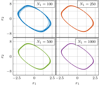
Figure 2: Randomized estimates $R_{N,q}$ of the set $\mathcal{R}_{25}$ for (20), (21) with varying sample sizes and polynomial degree $2q=4$.

We evaluate $R_{N,q}$ empirically at $M=$10\,000$$ sample points $x\in\mathcal{D}$ for each estimate. We are interested in those samples that lie in $\mathcal{R}_{25}$ but not in $R_{N,q}$ (false-negative), and those that lie outside $\mathcal{R}_{25}$ but within $R_{N,q}$ (false-positive). For each sample size $N_{2}=2N_{1}$, the average and worst-case empirical probabilities (denoted by $\operatorname{P}_{M}\{\cdot\}$) are detailed in Tab. I. The rate of false-positive test points decreases for larger sample sizes, in agreement with the theoretical results, and is well below the predicted accuracies in all cases. The rate of false-negative test points (relative to $\mathcal{R}_{25}$) shows more variation for smaller samples than for larger, which is also to be expected.

TABLE I: Empirical accuracy of $R_{N,q}$ for (21) with varying sample sizes and degree $2q=4$ (results in $0.01$).

	$\operatorname{P}_{M}\{\mathcal{R}_{p}\setminus R_{N,q}$}		$\operatorname{P}_{M}\{R_{N,q}\setminus\mathcal{R}_{p}\}$
$N_{1}$	mean	max	mean	max
$100$	$0.0473$	$0.1405$	$0.0040$	$0.0168$
$250$	$0.0389$	$0.0690$	$0.0019$	$0.0048$
$500$	$0.0453$	$0.0892$	$0.0009$	$0.0031$
$1000$	$0.0441$	$0.0671$	$0.0004$	$0.0013$

VI-B Suboptimal MPC

We now turn our attention to a time-distributed optimal control scheme for the open-loop dynamics in (20). Let $z\in\mathbb{R}^{3}$ be a finite-horizon input sequence. The optimal MPC feedback is obtained by solving an optimal control problem parametrized in the initial condition $x$, namely, minimizing the finite-horizon ($T=3$) quadratic cost

$$\langle P\xi_{T},\xi_{T}\rangle+\sum_{k=0}^{T-1}\langle Q\xi_{k},\xi_{k}\rangle+\langle R\mu_{k},\mu_{k}\rangle$$

where $\{\xi_{k}\}_{k=0}^{T}$ is a solution to $\xi_{k+1}=A_{\text{op}}\xi_{k}+B\mu_{k}$ for all $k\in\{0,\ldots,T\}$ with $\xi_{0}=x$ under control inputs $\{\mu_{k}\}_{k=0}^{T-1}\subset[-1,1]$. The terminal weight $P$ is the solution to the discrete Riccati equation for $Q=I_{2}$ and $R=1$. Setting $z=(\mu_{0},\ldots,\mu_{T-1})$ and eliminating the state sequence algebraically, we obtain the quadratic program

$$\hat{z} \in\operatorname*{arg\,min}_{z\in[-1,1]^{3}}\langle Hz,z\rangle+\langle 2Gx,z\rangle$$ (22a)

$$\hat{u} =\begin{bmatrix}1&0&0\end{bmatrix}\,\hat{z}$$ (22b)

with suitable matrices $G\in\mathbb{R}^{T\times 2}$ and $H\in\mathbb{S}_{T}$ (see [4] for details).

We employ a suboptimal solution to (22) given by $r=25$ iterations of the projected-gradient descent algorithm

$$z_{i+1} =\Pi(z_{i}-2\alpha(Hz_{i}+Gx))$$ (23a)

$$\psi(x,z) =\begin{bmatrix}1&0&0\end{bmatrix}\,z_{r}\quad\text{if $z_{0}=z$}$$ (23b)

where $\Pi$ is the projection onto the input constraints. The closed-loop dynamics of (20) and (23) form a linear system with combined state $(x,z)$ under an extended nonlinear projection operator. We obtain $r_{\iota}=0.6132$ for $\tilde{p}=6$.

Choosing $z=0$ as initial guess, we estimate the set $\mathcal{R}_{250}$ with $c_{250}=94.3704$ restricted to the space of $x$. We run Algorithms 2 and 3 using $N_{1}=1500$ and $N_{2}=3000$ samples, respectively, and polynomial degrees $2q\in\{2,4,6,8\}$. Based on a reliability of $\delta_{1}=\delta_{2}=$1\text{\times}{10}^{-6}$$, these sample sizes correspond to an accuracy of $\epsilon_{2}=$0.0073$$ for inner estimation and accuracies $\epsilon_{1}\in[$0.0241$,$0.2519$]$, depending on $n_{q}$, for outer estimation (relative to the inner sublevel sets $\mathcal{R}^{\nu}$). Fig. 3 shows the estimates $R_{N,q}$ for the suboptimal MPC.

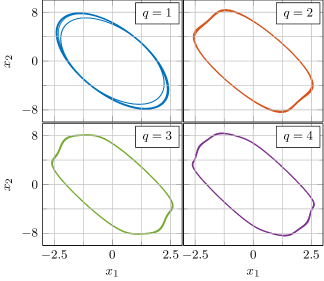
Figure 3: Randomized estimates $R_{N,q}$ of the set $\mathcal{R}_{250}$ for (20), (23) with $N_{1}=1500$, $N_{2}=3000$, and varying degree $2q$.

TABLE II: Empirical accuracy of $R_{N,q}$ for (20), (23) with $N_{1}=1500$, $N_{2}=3000$, and varying degree $2q$ (results in $0.01$).

	$\operatorname{P}_{M}\{\mathcal{R}_{p}\setminus R_{N,q}$}		$\operatorname{P}_{M}\{R_{N,q}\setminus\mathcal{R}_{p}\}$
degree	mean	max	mean	max
$q=1$	$0.1185$	$0.1920$	$0.000\,44$	$0.001\,84$
$q=2$	$0.0576$	$0.0726$	$0.000\,15$	$0.000\,47$
$q=3$	$0.0327$	$0.0412$	$0.000\,20$	$0.000\,57$
$q=4$	$0.0160$	$0.0227$	$0.000\,29$	$0.000\,56$

For each degree $q$, the average and worst-case empirical probabilities are detailed in Tab. II. It is shown that the rate of false-positive samples remains well below the accuracy of the inner estimation predicted by Theorem 2. The rate of false-negative samples (relative to $\mathcal{R}_{p}$) appears to decrease with increasing polynomial degrees, even though $N_{1}$ was constant. It is important to note that the apparent fluctuation in the false-positive rate does not contradict our theoretical results but can be explained by reduced conservatism of the estimates $R_{N,q}$.

VII Conclusion

Data-driven stability estimates previously lacked probabilistic guarantees, had sample complexities scaling badly for larger systems, or provided only conservative approximations. Combining empirical optimization with ideas from converse Lyapunov theory, we have proposed an hierarchical, data-driven region-of-attraction estimation. While at each level the polynomial estimate is a probabilistic inner approximation of some desired accuracy, with sample complexity independent of the number of states or polynomial degree, we have proven that the estimates also converge in probability to be outer approximations. Thus, our approach is both accurate and non-conservative.

Appendix A

We propose a simple but efficient method for a lower bound on $\tilde{r}$ guaranteeing that $\mathscr{B}(\tilde{r})$ is $\tilde{p}$-invariant. To that extent, write $\phi$ as

$$\phi=B_{1}\circ\phi_{1}\circ K_{1}+\cdots+B_{m}\circ\phi_{m}\circ K_{m}$$ (24)

with $m\in\mathbb{N}$, where $\phi_{1},\ldots,\phi_{m}:\mathbb{R}\to\mathbb{R}$ are scalar nonlinear functions and $\{(B_{i},K_{i}^{\mathrm{T}})\in\mathbb{R}^{n}\times\mathbb{R}^{n}\}_{i=1}^{m}$ are pairs of linear operators. We make the following assumptions.

Assumption 3

$\phi_{1},\ldots,\phi_{m}$ are monotonic functions satisfying $|\phi_{i}(w)|\leq\phi_{i}(|w|)$ for all $w\in\mathbb{R}$ and $i\in\{1,\ldots,m\}$.

Let $\{x_{k}\}_{k\geq 0}$ be a solution of $\Pi(x_{0})$ for an arbitrary initial condition $x_{0}\in\mathbb{R}^{n}$ and define $w_{p,i}=K_{i}x_{p}$ for all $p\geq 0$ and $i\in\{1,\ldots,m\}$; we bound the state norm after $p\geq 0$ steps as

$$\|x_{p}\|_{2}\leq\|A^{p}\|\,r+\sum_{p^{\prime}=0}^{p-1}\sum_{i=1}^{m}||A^{p-p^{\prime}-1}B_{i}||\,\phi_{i}(|w_{p^{\prime},i}|)$$ (25)

if $r=\|x_{0}\|_{2}$, where the $i$-th output after any $p^{\prime}<p$ steps satisfies the recursive bound

$$|w_{p^{\prime},i}|\leq||K_{i}A^{p^{\prime}}||\,r+\sum_{p^{\prime\prime}=0}^{p^{\prime}-1}\sum_{i^{\prime}=1}^{m}|K_{j}A^{p^{\prime}-p^{\prime\prime}-1}B_{i}|\,\phi_{i}(|w_{p^{\prime\prime},i^{\prime}}|)$$

and in particular, $|w_{0,i}|\leq||K_{i}||\,r$, for all $i\in\{1,\ldots,m\}$. In other words, there exists a monotonic scalar bound

$$\|x_{p}\|_{2}\leq F_{p}(r)$$ (26)

for all $x_{0}\in\mathscr{B}(r)$.

A sequence of lower bounds $r_{\iota}<\tilde{r}$ for $\tilde{p}>0$ can then be found as solutions to the family of optimization problems

$$r_{\iota}=\max\{r\geq 0\,|\,F_{p}(r)\leq r-\iota,\;p\in\{\tilde{p},\ldots,2\tilde{p}-1\}\}$$

for $\iota>0$, satisfying $\mathscr{B}(r_{\iota})\subset\mathscr{B}(\tilde{r})$.

Proposition 6

Let $\iota>0$ be small; if $\|A^{p}\|<1$ for all $p\geq\tilde{p}$ and $\phi_{i}(|w|)|\leq|w|^{\alpha}$ on $w\in\mathbb{R}$ for all $i\in\{1,\ldots,m\}$ and some $\alpha>1$, then $r_{\iota}$ exists and satisfies $r_{\iota}>0$.

Proof:

Replacing $\phi_{i}(\cdot)$ in (25), we obtain

$$F_{p}(r)\leq\gamma r+\beta|r|^{\alpha}$$

with $\gamma,\beta>0$ for all $p\in\{\tilde{p},\ldots,2\tilde{p}-1\}$; moreover, if $\|A^{p}\|<1$ for all $p\geq\tilde{p}$, we can choose $\gamma<1$. If $\alpha>1$, then there exists $r^{*}>0$ such that $\gamma r+\beta|r|^{\alpha}<r$ for all $r\in(0,r^{*})$ and hence, if $\iota$ is sufficiently small, $F_{p}(r^{\prime})\leq r^{\prime}-\iota$ for some $r^{\prime}\in(0,r^{*})$. In other words, $r_{\iota}$ is the maximum of a nonempty set and $r_{\iota}\geq r^{\prime}$, the desired result. ∎

The sufficient condition in Proposition 6 are satisfied for any stable matrix $A$ (compare [17, Proposition 3.1] and functions such as $w\mapsto w-\operatorname{sat}(w)$ or $w\mapsto w-\tanh(w)$, which are obtained in the analysis of optimization algorithms and neural network control, respectively.

Appendix B

The following, auxiliary results are used to prove uniqueness of the polynomial approximation.

B-A Spanning the normal cone

Let the convex set $K\subset\mathbb{R}^{n_{\xi}}$ satisfy

$$K\subseteq\{\xi\in\mathbb{R}^{n_{\xi}}\,|\,A\xi\leq b\}$$

for some $A\in\mathbb{R}^{m\times n_{\xi}}$ and $b\in\mathbb{R}^{m}$. The normal cone of $K$ is defined as

$$N_{K}(\bar{\xi})=\{y\in\mathbb{R}^{n_{\xi}}\,|\,\text{$\langle y,\bar{\xi}-\xi\rangle\geq 0$ for all $\xi\in K$}\}$$ (27)

for any point $\bar{\xi}\in K$.

Lemma 7

Let $\bar{\xi}\in K$ satisfy $A\bar{\xi}=b$ and $y\in\mathbb{R}^{n_{\xi}}$; there exist $\lambda\in\mathbb{R}_{\geq 0}^{m}$ such that $y=A^{\mathrm{T}}\lambda$ if and only if $y\in N_{K}(\bar{\xi})$.

Proof:

Take $\lambda\geq 0$, then $\langle A^{\mathrm{T}}\lambda,\bar{\xi}-\xi\rangle=\langle\lambda,b-A\xi\rangle\geq 0$ for any $\xi\in\mathbb{R}^{n_{\xi}}$ satisfying $A\xi\leq b$ (i.e., for any $\xi\in K$) and hence, $A^{\mathrm{T}}\lambda\in N_{K}(\bar{\xi})$. To see the opposite direction, assume that no such $\lambda\geq 0$ exists for $y\in\mathbb{R}^{n_{\xi}}$; by Farkas’ lemma, then $A\nu\geq 0$ and $\langle y,\nu\rangle<0$. Since $A(\bar{\xi}-\nu)\leq b$ we have that $y\not\in N_{K}(\bar{\xi})$, the desired result. ∎

Note that, in the main part, the inequalities were flipped for both $K_{2}$ and $N^{-}_{K}(\bar{\xi})$, thus recovering the result.

B-B Linear independence of monomials

Let $x^{(1)},\ldots,x^{(N)}$ be $N\in\mathbb{N}$ samples of a random variable $x\in\mathbb{R}^{n}$ and define the matrix

$$S_{q}(x)=\begin{bmatrix}Z_{q}\{x^{(1)}\}&\cdots&Z_{q}\{x^{(N)}\}\end{bmatrix}\in\mathbb{R}^{n_{q}\times N}$$

where $Z_{q}\{x\}\in\mathbb{R}^{n_{q}}$ denotes the vector of monomials of $x$ (starting with $x^{0}\equiv 1$) up to degree $q\in\mathbb{N}$. We assume without loss of generality that $N=n_{q}$. The following statements are equivalent [28, Theorem 4]:

1. The matrix $S_{q}(x)$ has full rank;

2. The points $x^{(1)},\ldots,x^{(N)}$ do not belong to a common algebraic hypersurface $\langle\psi,Z_{q}\{x\}\rangle=0$ with $\psi\neq 0$;

3. The interpolation $S_{q}(x)^{\mathrm{T}}\theta=v$ has a unique solution for any $v\in\mathbb{R}^{N}$.

Note that these statements are equivalent to the null space of $S_{q}(x)$ being equal to $\{0\}$. They also hold independently of the actual elements or ordering of $Z_{q}\{x\}$. This allows to prove the following result by induction.

Proposition 7

The matrix $S_{q}(x)$ has almost surely full rank.

Proof:

We show that any top-left $k\times k$ block $S^{[k]}$ of $S_{q}(x)$ with $k\in\{1,\ldots,n_{q}\}$ has full rank with probability one: Clearly, this is true for $S^{[1]}=1$.

Assume that $S^{[k]}$ has full rank; consequently, the top-left $(k+1)\times k$ block $S^{[k]}{}^{\prime}$ of $S_{q}(x)$ has a null space spanned by $\psi\in\mathbb{R}^{k+1}-\{0\}$. In other words, the samples $x^{(1)},\ldots,x^{(k)}$ belong to the unique algebraic hypersurface $\langle(\psi,0),Z_{q}\{x\}\rangle=0$. However, the probability that $x^{(k+1)}$ belongs to the same hypersurface is zero and hence, $S^{[k+1]}$ has full rank with probability one. Repeating this argument until $k=n_{q}$ completes the proof. ∎

Since there are finitely many permutations of $N$ samples, we conclude that any combination of up to $n_{q}$ sampled vectors of monomials is linearly independent with probability one if $N>n_{q}$.

References

- [1] R. Genesio, M. Tartaglia, and A. Vicino, “On the Estimation of Asymptotic Stability Regions: State of the Art and New Proposals,” IEEE Transactions on Automatic Control, vol. 30, no. 8, pp. 747–755, 1985.
- [2] T. Cunis and I. Kolmanovsky, “Viability, viscosity, and storage functions in model-predictive control with terminal constraints,” Automatica, vol. 131, p. 109748, 2021.
- [3] T. Skibik, D. Liao-McPherson, T. Cunis, I. V. Kolmanovsky, and M. M. Nicotra, “A Feasibility Governor for Enlarging the Region of Attraction of Linear Model Predictive Controllers,” IEEE Transactions on Automatic Control, vol. 67, no. 10, pp. 5501–5508, 2022. [Online]. Available: http://arxiv.org/abs/2011.01924
- [4] J. Leung, D. Liao-McPherson, and I. V. Kolmanovsky, “A Computable Plant-Optimizer Region of Attraction Estimate for Time-distributed Linear Model Predictive Control,” in Proceedings of the American Control Conference, 2021, pp. 3384–3391.
- [5] N. Hashemi, J. Ruths, and M. Fazlyab, “Certifying Incremental Quadratic Constraints for Neural Networks via Convex Optimization,” arXiv, no. 2012.05981, 2020. [Online]. Available: http://arxiv.org/abs/2012.05981
- [6] H. Yin, P. Seiler, and M. Arcak, “Stability Analysis using Quadratic Constraints for Systems with Neural Network Controllers,” IEEE Transactions on Automatic Control, vol. 9286, no. 1, 2021.
- [7] M. Fazlyab, M. Morari, and G. J. Pappas, “Safety Verification and Robustness Analysis of Neural Networks via Quadratic Constraints and Semidefinite Programming,” IEEE Transactions on Automatic Control, 2020.
- [8] U. Topcu, A. Packard, and P. Seiler, “Local stability analysis using simulations and sum-of-squares programming,” Automatica, vol. 44, no. 10, pp. 2669–2675, 2008.
- [9] A. Chakraborty, P. Seiler, and G. J. Balas, “Nonlinear region of attraction analysis for flight control verification and validation,” Control Engineering Practice, vol. 19, no. 4, pp. 335–345, 2011.
- [10] H. Yin, A. Packard, M. Arcak, and P. Seiler, “Finite horizon backward reachability analysis and control synthesis for uncertain nonlinear systems,” in Proceedings of the American Control Conference, Philadelphia, US-PA, 2019, pp. 5020–5026.
- [11] B. K. Colbert and M. M. Peet, “Using Trajectory Measurements to Estimate the Region of Attraction of Nonlinear Systems,” in Proceedings of the IEEE Conference on Decision and Control. IEEE, 2018, pp. 2341–2347.
- [12] B. Lai, T. Cunis, and L. Burlion, “Nonlinear Trajectory Based Region of Attraction Estimation for Aircraft Dynamics Analysis,” in AIAA Scitech Forum 2021, Virtual, 2021.
- [13] R. Tempo, G. Calafiore, and F. Dabbene, Randomized Algorithms for Analysis and Control of Uncertain Systems, 2nd ed. London: Springer, 2013.
- [14] A. Devonport and M. Arcak, “Estimating Reachable Sets with Scenario Optimization,” in Proceedings of the 2nd Conference on Learning for Dynamics and Control, ser. Proceedings of Machine Learning Research, no. 120, The Cloud, 2020, pp. 75–84.
- [15] M. Korda, “Computing Controlled Invariant Sets from Data Using Convex Optimization,” SIAM Journal on Control and Optimization, vol. 58, no. 5, pp. 2871–2899, 2020.
- [16] Y. Shen, M. Bichuch, and E. Mallada, “Model-free Learning of Regions of Attraction via Recurrent Sets,” pp. 1–9, 2022. [Online]. Available: http://arxiv.org/abs/2204.10372
- [17] S. T. Balint, E. Kaslik, A. M. Balint, and A. Grigis, “Methods for determination and approximation of the domain of attraction in the case of autonomous discrete dynamical systems,” Advances in Difference Equations, vol. 2006, no. 23939, pp. 1–15, 2006.
- [18] A. Kalur, T. Mushtaq, P. Seiler, and M. S. Hemati, “Estimating Regions of Attraction for Transitional Flows Using Quadratic Constraints,” IEEE Control Systems Letters, vol. 6, no. 2, pp. 482–487, 2022.
- [19] L. Khodadadi, B. Samadi, and H. Khaloozadeh, “Estimation of region of attraction for polynomial nonlinear systems: A numerical method,” ISA Transactions, vol. 53, no. 1, pp. 25–32, 2014.
- [20] M. Jones, H. Mohammadi, and M. M. Peet, “Estimating the region of attraction using polynomial optimization: A converse Lyapunov result,” in 56th IEEE Conference on Decision and Control, Melbourne, AU, 2017, pp. 1796–1802.
- [21] J. M. Ortega, “Stability of Difference Equations and Convergence of Iterative Processes,” SIAM Journal on Numerical Analysis, vol. 10, no. 2, pp. 268–282, 1973.
- [22] Z. P. Jiang and Y. Wang, “A converse Lyapunov theorem for discrete-time systems with disturbances,” Systems and Control Letters, vol. 45, no. 1, pp. 49–58, 2002.
- [23] Z. Zeng, “Converse Lyapunov Theorems for Nonautonomous Discrete-Time Systems,” Journal of Mathematical Sciences, vol. 161, no. 2, pp. 337–343, 2009.
- [24] R. Geiselhart, R. H. Gielen, M. Lazar, and F. R. Wirth, “An alternative converse Lyapunov theorem for discrete-time systems,” Systems and Control Letters, vol. 70, pp. 49–59, 2014.
- [25] L. Blum, F. Cucker, M. Shub, and S. Smale, Complexity and Real Computation. New York, NY: Springer, 1998.
- [26] W. Cheney and W. Light, A Course in Approximation Theory, ser. Graduate Studies in Mathematics. Providence, Rhode Island: American Mathematical Society, 2000, vol. 101.
- [27] O. L. Mangasarian, “Uniqueness of solution in linear programming,” Linear Algebra and Its Applications, vol. 25, no. C, pp. 151–162, 1979.
- [28] P. J. Olver, “On multivariate interpolation,” Studies in Applied Mathematics, vol. 116, no. 2, pp. 201–240, 2006.