Abstract

Gaussian distributions are widely used in Bayesian variational inference to approximate intractable posterior densities, but the ability to accommodate skewness can improve approximation accuracy significantly, especially when data or prior information is scarce. We study the properties of a subclass of closed skew normals constructed using affine transformation of independent standardized univariate skew normals as the variational density, and illustrate how this subclass provides increased flexibility and accuracy in approximating the joint posterior density in a variety of applications by overcoming limitations in existing skew normal variational approximations. The evidence lower bound is optimized using stochastic gradient ascent, where analytic natural gradient updates are derived. We also demonstrate how problems in maximum likelihood estimation of skew normal parameters occur similarly in stochastic variational inference and can be resolved using the centered parametrization.

keywords: Closed skew normal; Gaussian variational approximation; natural gradient; centered parametrization; LU decomposition

1 Introduction

Variational inference (Ormerod and Wand, 2010; Blei et al., 2017) is a popular and scalable alternative to Markov chain Monte Carlo (MCMC) methods for deriving approximate Bayesian inference. Given observed data $y$, the intractable posterior density $p(\theta|y)$ of the variables $\theta$ is approximated by a variational density $q(\theta)$, which is assumed to satisfy some restrictions such as lying in a parametric family or being of a factorized form (variational Bayes, Attias, 1999). The Kullback-Leibler (KL) divergence between the true posterior and variational density is then minimized under these constraints. As

$$\log p(y)=\underbrace{\int q(\theta)\log\frac{p(y,\theta)}{q(\theta)}d\theta}_{\text{Evidence lower bound}}+\underbrace{\int q(\theta)\log\frac{q(\theta)}{p(\theta|y)}d\theta}_{\text{KL divergence}},$$ (1)

this is equivalent to maximizing an evidence lower bound on the log marginal likelihood. Variational Bayes is widely applied due to the availability of analytic coordinate ascent updates for models with conditionally conjugate priors (Braun and McAuliffe, 2010; Durante and Rigon, 2019; Ray and Szabo, 2022) and its scalability to massive data sets via subsampling (Hoffman et al., 2013; Kabisa et al., 2016). Frequentist consistency and asymptotic normality of variational Bayes have been established (Wang and Blei, 2019). However, assuming independence among variables which are strongly correlated a posteriori can result in underestimation of posterior variance (Turner and Sahani, 2011), and dependencies among variables can be restored through structured (Salimans and Knowles, 2013; Hoffman and Blei, 2015) and copula variational inference (Tran et al., 2015; Han et al., 2016). Saha et al. (2020) minimized the Rényi-$\alpha$ instead of the KL divergence on the nonparametric manifold of probability densities equipped with the Riemannian Fisher-Rao metric, leading to a tighter evidence lower bound. Tan (2021) introduced reparametrized variational Bayes for hierarchical models, where local variables are first transformed to be approximately independent of the global variables via a second order Taylor approximation of their conditional posterior. For high-dimensional Bayesian probit regression, Fasano et al. (2022) proposed a partially factorized variational Bayes approximation where latent variables are assumed to be independent, but global variables are allowed to depend on latent variables. A hybrid variational approximation for state space models was introduced in Loaiza-Maya et al. (2022), where the marginal posterior of global variables is approximated using Gaussian copula while latent variables are sampled conditionally on global variables using MCMC.

Gaussian variational approximation (Opper and Archambeau, 2009), where the posterior density is approximated jointly by a Gaussian, is another popular and broadly applicable approach (Tan and Friel, 2020; Quiroz et al., 2022) that captures posterior correlation among variables. It is the only option for variational inference in Stan (Stan Development Team, 2023), implemented via automatic differentiation variational inference (Kucukelbir et al., 2016), and transformations can be applied in advance to improve the normality of constrained or skewed variables (Yeo and Johnson, 2000; Yan and Genton, 2019). As the number of variational parameters scale as the square of the dimension of the Gaussian density, Tan and Nott (2018) used a sparse precision matrix to capture posterior conditional independence relationships, while Ong et al. (2018) considered a factor covariance structure, and Zhou et al. (2021) applied Stiefel and Grassmann manifold constraints. Although Gaussian variational approximations are supported asymptotically by the Bernstein-von Mises theorem (Doob, 1949; van der Vaart, 2000) stating that posterior densities in parametric models converge to a Gaussian at $\mathcal{O}(1/\sqrt{n})$, moderately large sample sizes may be required before the posterior will resemble a Gaussian closely.

Anceschi et al. (2023) showed that the posteriors induced by the probit, tobit and multinomial probit models belong to the class of unified skew normal distributions (Arellano-Valle and Azzalini, 2006). In addition, Durante et al. (2023) proved the skewed Bernstein-von Mises theorem showing that posterior distributions in regular parametric models converge to the generalized skew normal distribution (Genton and Loperfido, 2005) at a faster rate of $\mathcal{O}(1/n)$, and obtained a skew-modal approximation via a maximum-a-posteriori estimate plug-in. To improve upon the Gaussian variational approximation and account for skewness, Ormerod (2011), Lin et al. (2019) and Zhou et al. (2023) considered the multivariate skew normal (Azzalini and Capitanio, 1999) as the variational density, while Smith et al. (2020) used it to construct implicit copulas. Ormerod (2011) used the BFGS algorithm (Nocedal and Wright, 1999) to maximize the lower bound numerically while Lin et al. (2019) used stochastic natural gradient ascent, and Zhou et al. (2023) matched key statistic estimates of the posterior with those of the skew normal. Salomone et al. (2023) considered skew decomposable graphical models (Zareifard et al., 2016) for variational inference, and used the Cholesky factor of the precision matrix to capture conditional independence in the posterior.

In this article, we consider a subclass of closed skew normals (González-Farías et al., 2004), constructed via affine transformations of independent univariate skew normals as the variational density. This subclass falls in the framework of affine independent variational inference (Challis and Barber, 2012), and has attractive inferential properties such as closed form expressions for its moments and marginal densities, while being sufficiently flexible in approximating joint posterior densities in that a bounding line is permitted in each dimension, unlike the skew normal whose tail is bounded by a single line (Sahu et al., 2003). Several novel contributions are made. First, we show that the evidence lower bound of the closed skew normal subclass has a stationary point when the skewness parameter $\lambda$ equals zero, and that problems encountered in maximum likelihood estimation of skew normal parameters due to this stationary point (Azzalini, 1985; Azzalini and Capitanio, 1999) persist in stochastic variational inference. Peculiar behavior of the likelihood function of the skew normal at $\lambda=0$ is well known. Besides the stationary point, the Fisher information is also singular at $\lambda=0$ due to a mismatch between the symmetric kernel and skewing function (Hallin and Ley, 2012, 2014). Second, we demonstrate that using a parametrization composed of the mean, transformed skewness and a decomposition of the covariance matrix, akin to the “centered parametrization” proposed by Arellano-Valle and Azzalini (2008), is effective in resolving optimization issues due to the stationary point at $\lambda=0$. Third, we derive analytic natural gradients for optimizing the evidence lower bound using stochastic gradient ascent by considering a data augmentation scheme and a parametrization that ensures positive definiteness of the covariance matrix. The natural gradient (Amari, 2016) takes into account the curvature of the parameter space and can help to accelerate convergence. Finally, we demonstrate that this subclass exhibits flexibility and improved accuracy in approximating the joint posterior density in a variety of statistical applications.

First, we review the multitude of multivariate skew normal distributions that now exist and discuss properties of the proposed closed skew normal subclass in Section 2. In Section 3, we examine issues that arise in optimization of the evidence lower bound and illustrate them using examples where the lower bound can be evaluated (almost) exactly. We proceed to the general case where the lower bound is intractable and present the Euclidean and natural gradients for stochastic variational inference in Section 4. The performance of the closed skew normal subclass is evaluated in a variety of statistical applications in Section 5.1. Finally, Section 6 concludes with a discussion.

2 Multivariate skew normal distributions

The original multivariate skew normal (SN, Azzalini and Capitanio, 1999) is well-studied and has been considered as a variational density by Ormerod (2011), Lin et al. (2019) and Zhou et al. (2023). The probability density function (pdf) of $\theta\sim{\text{SN}}_{d}(\mu,\Sigma,\lambda)$ is

$$p(\theta)=2\phi_{d}(\theta|\mu,\Sigma)\Phi\{\lambda^{T}(\theta-\mu)\},$$ (2)

where $\mu\in\mathbb{R}^{d}$ and $\lambda\in\mathbb{R}^{d}$ represent the location and shape parameters respectively and $\Sigma$ is a $d\times d$ symmetric positive definite matrix. Let $\phi_{d}(\cdot|\mu,\Sigma)$ denote the $d$-dimensional Gaussian density with mean $\mu$ and covariance matrix $\Sigma$, and $\Phi(\cdot)$ the cumulative distribution function (cdf) of the univariate standard normal. The mean is ${\text{E}}(\theta)=\mu+b\delta_{s}$ where $b=\sqrt{2/\pi}$ and $\delta_{s}=\Sigma\lambda/\sqrt{1+\lambda^{T}\Sigma\lambda}$, and $\text{\rm Var}(\theta)=\Sigma-b^{2}\delta_{s}\delta_{s}^{T}$. If

$$\begin{bmatrix}\theta_{0}\\ \theta_{1}\end{bmatrix}\sim{\text{N}}(0,\Sigma_{s}),\quad\Sigma_{s}=\begin{bmatrix}1&\delta_{s}^{T}\\ \delta_{s}&\Sigma\end{bmatrix},\quad\theta_{0}\in\mathbb{R},\theta_{1}\in\mathbb{R}^{d},$$

then $\theta$ can be represented stochastically (Arellano-Valle and Azzalini, 2006) as $\theta=\theta_{1}|\theta_{0}>0$. To analyze the role of the shape parameter $\lambda=(\lambda_{1},\dots,\lambda_{d})^{T}$, we set $\mu=0$ and $\Sigma=I_{d}$. In Figure 1, the univariate densities become increasingly skewed as the magnitude of $\lambda$ increases. For the contours plots of the bivariate skew normal densities, the angle of inclination is captured by the ratio of $\lambda_{1}$ and $\lambda_{2}$ while the degree of flattening against the bounding line is controlled by their magnitude.

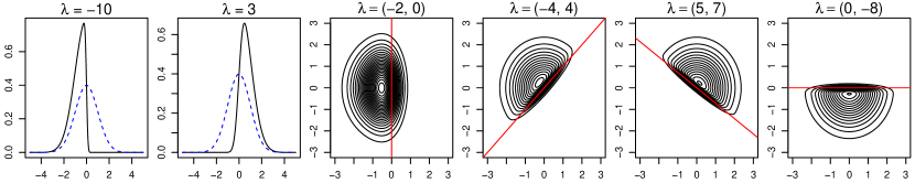
Figure 1: First two plots show univariate skew normal densities. Standard normal is added in blue dashed lines for comparison. Last four are contour plots of bivariate skew normal densities and the bounding red line has gradient $-\lambda_{1}/\lambda_{2}$.

For the same gradient, the densities become more flattened as $|\lambda_{i}|$ increases. While any angle of inclination can be achieved by varying $\lambda$, densities that are bounded in more than one direction cannot be captured. This characteristic of the skew normal becomes more limiting as the dimension $d$ increases and impedes its ability to provide accurate variational approximations. This constraint is due to $\theta$ being constructed as $\theta_{1}$ conditioned on only one random variable $\theta_{0}$ being positive, and Sahu et al. (2003) propose conditioning on $d$ random variables instead where $d$ is the dimension of $\theta$.

More generally, González-Farías et al. (2004) introduced the closed skew normal (CSN) distribution, which is constructed by conditioning on $q$ random variables. The pdf of $\theta\sim{\text{CSN}}_{d,q}(\mu,\Sigma,D,\nu,\Delta)$ is

$$p(\theta)=\phi_{d}(\theta|\mu,\Sigma)\frac{\Phi_{q}(D(\theta-\mu)|\nu,\Delta)}{\Phi_{q}(0|\nu,\Delta+D\Sigma D^{T})},$$

where $\mu\in\mathbb{R}^{d}$, $\nu\in\mathbb{R}^{q}$, $D$ is a $q\times d$ matrix, $\Sigma$ and $\Delta$ are $d\times d$ and $q\times q$ positive definite matrices respectively and $\Phi_{q}(\cdot|\mu,\Sigma)$ denotes cdf of a $q$-dimensional normal random vector with mean $\mu$ and covariance matrix $\Sigma$. As its name suggests, the CSN enjoys many closure properties akin to the normal distribution, which are made possible by inclusion of the $q$-dimensional cdf and extra parameters $\nu$ and $\Delta$. For instance, the CSN is closed under the sum of independent CSN random vectors (a property absent for the skew normal) and affine transformation. From Proposition 2.3.1 of González-Farías et al. (2004), if $A$ is a $p\times d$ matrix of rank $p\leq d$ and $c$ is a vector of length $p$, then

$$A\theta+c\sim{\text{CSN}}_{p,q}(A\mu+c,\Sigma_{A},D_{A},\nu,\Delta_{A}),$$ (3)

where $\Sigma_{A}=A\Sigma A^{T}$, $D_{A}=D\Sigma A^{T}\Sigma_{A}^{-1}$ and $\Delta_{A}=\Delta+D\Sigma D^{T}-D\Sigma A^{T}\Sigma_{A}^{-1}A\Sigma D^{T}$. If $p=d$ and $A$ is invertible, then the simplification $D_{A}=DA^{-1}$ and $\Delta_{A}=\Delta$ applies. Arellano-Valle and Azzalini (2006) proposed an alternative formulation of the CSN known as the “unified skew normal” and discussed the connections among existing skew normal proposals.

The CSN is attractive due to its flexibility and closure properties, but the evaluation of $\Phi_{q}$ can be challenging for large $q$ (Genton et al., 2018). To develop a fast and flexible variational approximation, we consider CSN distributions where $q=d$, and $\Delta$ and $\Delta+D\Sigma D^{T}$ are both diagonal matrices. In this way, the variational approximation remains reasonably flexible as it can capture densities with a bounding line in each dimension. It can also be optimized efficiently since $\Phi_{q}(\cdot|\mu,\Sigma)$ can be computed as a product of $q$ univariate cdfs when $\Sigma$ is diagonal. Motivated by Márquez-Urbina and González-Farías (2022), we construct a CSN subclass via transformation of independent univariate skew normals to form the variational approximation in the next section.

2.1 A closed skew normal subclass

For $i=1,\dots,d$, let $v_{i}\sim{\text{SN}}_{1}(0,1,\lambda_{i})$ independently. Then the pdf of $v=(v_{1},\dots,v_{d})^{T}$ is

$$p(v)=2^{d}\phi_{d}(v|0,I_{d})\Phi_{d}(D_{\lambda}v),$$

where $D_{\lambda}=\text{\rm diag}(\lambda)$, $\lambda=(\lambda_{1},\dots,\lambda_{d})^{T}$ and $\Phi_{d}(x)=\Phi_{d}(x|0,I_{d})=\prod_{i=1}^{d}\Phi(x_{i})$ for any $x=(x_{1},\dots,x_{d})^{T}$. Let $\delta=(\delta_{1},\dots,\delta_{d})^{T}$ and $\tau=(\tau_{1},\dots,\tau_{d})^{T}$ where $\delta_{i}=\lambda_{i}/\sqrt{1+\lambda_{i}^{2}}$ and $\tau_{i}=\sqrt{1-b^{2}\delta_{i}^{2}}$, and $D_{\tau}=\text{\rm diag}(\tau)$. Then $v\sim{\text{CSN}}_{d,d}(0,I_{d},D_{\lambda},0,I_{d})$, where ${\text{E}}(v)=b\delta$ and $\text{\rm Var}(v)=D_{\tau}^{2}$. First we standardize $v$ by defining

$$z=D_{\tau}^{-1}(v-b\delta),$$

so that ${\text{E}}(z)=0$ and $\text{\rm Var}(z)=I_{d}$. To construct a CSN random vector $\theta$ with mean $\mu$ and covariance matrix $\Sigma=CC^{T}$, we define an affine transformation,

$$\theta =\mu+Cz,$$

where $\mu\in\mathbb{R}^{d}$ represents the translation and $C$ is a $d\times d$ invertible matrix representing the linear map. Since the CSN is closed under affine transformation,

$$\theta\sim{\text{CSN}}_{d,d}(\mu^{*},\Sigma^{*},D^{*},0,I_{d})$$

from (3), where $\mu^{*}=\mu-bC\alpha$, $\Sigma^{*}=CD_{\tau}^{-2}C^{T}$, $D^{*}=D_{\lambda}D_{\tau}C^{-1}$ and $\alpha=D_{\tau}^{-1}\delta$. The pdf is

$$q(\theta)=2^{d}\phi(\theta|\mu^{*},\Sigma^{*})\Phi_{d}\{D^{*}(\theta-\mu^{*})\},$$ (4)

and $q(\theta)$ reduces to ${\text{SN}}_{1}(\mu-b\sigma\alpha,\sigma^{2}/\tau^{2},\lambda\tau/\sigma)$ where we write $C$ as $\sigma$ if $d=1$. For $d>1$, $q(\theta)$ does not coincide with the skew normal. Based on the transformation of $\theta$ from $v$, we can also write $q(\theta)=p(v)|C^{-1}||D_{\tau}|$. Then

$$\log q(\theta)=d\log(2)-\frac{d}{2}\log(2\pi)-\frac{v^{T}v}{2}-\log|C|+\sum_{i=1}^{d}\{\log\Phi(\lambda_{i}v_{i})+\log\tau_{i}\},$$ (5)

where $v=D_{\tau}C^{-1}(\theta-\mu)+b\delta$. This CSN subclass falls in the affine independent variational inference framework (Challis and Barber, 2012), but its properties have not been studied in detail. Challis and Barber (2012) fit the variational approximation for a class of nonconjugate models using fast Fourier transform, while we do not impose any model restrictions and the lower bound is optimized using stochastic (natural) gradient ascent. Another related approach is by Salomone et al. (2023), but they consider a Cholesky decomposition of the precision instead of covariance matrix. As described in Section 2.2, we observe limitations to the fit of the variational approximation when $C$ is constrained to be triangular.

2.2 Decomposition of covariance matrix

Figure 2 shows some bivariate densities of the CSN subclass with $\mu=0$ and $C=I_{2}$. Compared to the skew normal densities in Figure 1, we can now capture fan-shaped densities with two bounding lines, although the number of bounding lines reduce to one if either $\lambda_{1}$ or $\lambda_{2}$ is zero. While the shape of densities that can be fitted by $q(\theta)$ has increased in range, Figure 2 highlights a limitation in the role of $\lambda$. In Figure 1, the bounding line can have any angle of inclination by varying $\lambda$, but it is not possible to rotate the densities in Figure 2 without altering the degree of flattening using $\lambda$. The role of rotation (and scaling) has thus fallen onto the linear map $C$.

Figure 2: Bivariate density contour plots of CSN subclass with $\mu=0$ and $C=I_{2}$.

For decomposition of the covariance matrix $\Sigma=CC^{T}$, a parametrization that ensures $\Sigma$ is positive definite and allows unconstrained optimization of the lower bound is desired. Two main approaches are Cholesky factorization and spectral decomposition (Pinheiro and Bates, 1996). A Cholesky factorization is more efficient computationally and independence assumptions can be imposed easily. If $\theta=(\theta_{1}^{T},\theta_{2}^{T})^{T}$ and $C=\text{\rm diag}(C_{11},C_{22})$ is a corresponding partitioning, then it is clear from (4) that $\theta_{1}$ and $\theta_{2}$ are independent. We can also impose conditional independence assumptions through Cholesky decomposition of $\Sigma^{-1}$ (Tan and Nott, 2018; Salomone et al., 2023), but a disadvantage of a Cholesky decomposition of $\Sigma$ or $\Sigma^{-1}$ is that $C$ will be a triangular matrix that is unable to capture rotations in every plane, resulting in suboptimal variational approximations. For instance, a 2-dimensional anti-clockwise rotation of $\omega$ about the origin is performed by

$$\begin{bmatrix}\cos(\omega)&-\sin(\omega)\\ \sin(\omega)&\cos(\omega)\end{bmatrix},$$

which cannot be triangular. We have also considered parametrizations based on Givens rotation matrices. As $\Sigma$ is positive definite and has $d$ positive eigenvalues, $\gamma_{1}^{2},\dots,\gamma_{d}^{2}$, we can write $\Sigma=QD_{\gamma}^{2}Q^{T}$, where $Q$ is an orthogonal matrix containing the orthonormal eigenvectors of $\Sigma$ and satisfies $QQ^{T}=Q^{T}Q=I_{d}$. We can represent $Q$ as the product of $d(d-1)/2$ Givens rotation matrices, $Q=(G_{12}\dots G_{1d})(G_{23}\dots G_{2d})\dots G_{d-1,d}$, where $G_{ij}$ is an identity matrix with four elements modified to become $G_{i,i}=G_{j,j}=\cos(\omega_{ij})$ and $G_{j,i}=-G_{i,j}=\sin(\omega_{ij})$. Each $G_{ij}$ is governed by a parameter $\omega_{ij}$ and thus $Q$ has $d(d-1)/2$ parameters while the number of parameters of $C=QD_{\gamma}$ is $d(d+1)/2$. The limitation is that all scalings are captured by $D_{\gamma}$ which must be performed prior to rotations represented by $Q$, but order matters and this restriction limits permissible transformations. Other disadvantages include the computational effort involved in finding $C$ given $\omega$, although the inverse can be obtained easily as $Q^{-1}=Q^{T}$.

As $CC^{T}$ is symmetric, our objective is to ensure $\Sigma$ remains positive definite and $C^{-1}$ can be computed efficiently during optimization. As the lower triangular structure does not permit rotations and is too restrictive, we consider $C$ to be a full $d\times d$ matrix and use the $LU$ decomposition so that it remains invertible efficiently. For uniqueness, we require the diagonal of $L$ or $U$ to consist of ones. In the rest of this article, we consider $C$ as a Cholesky factor or $C=LU$ where $L$ is lower triangular and $U$ is upper triangular with unit diagonal, and compare the variational approximations of these two options.

2.3 Properties of closed skew normal subclass

Next, we discuss some properties of this CSN subclass which forms the variational density. Let $C_{i\cdot}$ and $C_{\cdot j}$ respectively denote the $i$th row and $j$th column of a matrix $C$, $C_{ij}$ denote the $(i,j)$ element and define $\zeta_{r}(x)$ as the $r$th derivative of $\zeta_{0}(x)=\log\{2\Phi(x)\}$. Then $\zeta_{0}(0)=0$, $\zeta_{1}(0)=b$, $\zeta_{2}(0)=-b^{2}$ and $\zeta_{3}(0)=b(2b^{2}-1)$.

1. ${\text{E}}(\theta)=\mu$ and $\text{\rm Var}(\theta)=\Sigma=CC^{T}$ (by construction).

2. The cumulant generating function (log of the moment generating function) is

   $$K_{\theta}(t)=t^{T}\mu^{*}+\frac{1}{2}t^{T}\Sigma^{*}t+\sum_{j=1}^{d}\zeta_{0}(\alpha_{j}C_{\cdot j}^{T}t),\quad t\in\mathbb{R}^{d}.$$

   This result follows from Lemma 2.2.2 of González-Farías et al. (2004),

3. The marginal density of the $i$th element of $\theta$ is

   $$\theta_{i}\sim{\text{CSN}}_{1,d}(\mu^{*}_{i},\Sigma^{*}_{ii},D_{i},0,\Delta_{i}),$$

   where $\mu^{*}_{i}=\mu_{i}-bC_{i\cdot}^{T}\alpha$ is the $i$th element of $\mu^{*}$, $\Sigma^{*}_{ii}=b_{i}^{T}b_{i}$ is the $(i,i)$ element of $\Sigma^{*}$, $D_{i}=D_{\lambda}b_{i}/\Sigma^{*}_{ii}$, $\Delta_{i}=I_{d}+D_{\lambda}(I_{d}-b_{i}b_{i}^{T}/\Sigma^{*}_{ii})D_{\lambda}$ and $b_{i}=D_{\tau}^{-1}C_{i\cdot}$. This result can be obtained by setting $A$ as $e_{i}^{T}$ and $c=0$ in (3), where $e_{i}$ is a binary vector of length $d$ with only the $i$th element equal to one.

4. The marginal pdf of $\theta_{i}$ is

   $$q(\theta_{i})=2^{d}\phi(\theta_{i}|\mu^{*}_{i},\Sigma^{*}_{ii})\Phi_{d}(D_{i}(\theta_{i}-\mu_{i}^{*})|0,\Delta_{i}),$$

   which depends only on the parameters $\mu_{i}$, $C_{i\cdot}$ and $\lambda$. Note that $\Delta_{i}+D_{i}\Sigma^{*}_{ii}D_{i}^{T}=I_{d}+D_{\lambda}^{2}$, and hence the denominator in the pdf of the CSN, $\Phi_{d}(0|0,\Delta_{i}+D_{i}\Sigma^{*}_{ii}D_{i}^{T})=2^{-d}$. To evaluate $\Phi_{d}(\cdot)$ for large $d$, it may be useful to use the hierarchical Cholesky factorization approach in Genton et al. (2018).

5. The cumulant generating function of $\theta_{i}$ is $K_{\theta_{i}}(t)=\mu_{i}^{*}t+\tfrac{1}{2}\Sigma_{ii}^{*}t^{2}+\sum_{j=1}^{d}\zeta_{0}(\alpha_{j}C_{ij}t)$, $t\in\mathbb{R}$.

6. The marginal mean, variance and Pearson’s index of skewness of $\theta_{i}$ are $\mu_{i}$, $\Sigma_{ii}$ and $b(2b^{2}-1)(\sum_{j=1}^{d}\alpha_{j}^{3}C_{ij}^{3})/\Sigma_{ii}^{3/2}$ respectively.

7. To simulate from $q(\theta)$, we can employ the stochastic representation,

   $$\theta|w \sim{\text{N}}(\mu+CD_{\alpha}\widetilde{w},CD_{\kappa}^{2}C^{T}),$$

   $$w \sim{\text{N}}(0,I_{d}),$$

   where $\widetilde{w}=|w|-b{\bf 1}$, $|w|=(|w_{1}|,\dots,|w_{d}|)^{T}$, $D_{\alpha}=\text{\rm diag}(\alpha)$, $D_{\kappa}=\text{\rm diag}(\kappa)$ and $\kappa=(\kappa_{1},\dots,\kappa_{d})^{T}$ where $\kappa_{i}=1/\sqrt{1+(1-b^{2})\lambda_{i}^{2}}$. This result arises from the stochastic representation of $v_{i}\sim{\text{SN}}_{1}(0,1,\lambda_{i})$ as $v_{i}=|v_{0}|\delta_{i}+\sqrt{1-\delta_{i}^{2}}v_{1}$ where $v_{0},v_{1}\sim{\text{N}}(0,1)$ independently (Arellano-Valle and Azzalini, 2006). Therefore, to simulate from $q(\theta)$, we can generate $w_{1}$ and $w_{2}$ independently from ${\text{N}}(0,I_{d})$ and set

   $$\theta=C(D_{\kappa}w_{2}+D_{\alpha}\widetilde{w}_{1})+\mu,$$

   where $\widetilde{w}_{1}=|w_{1}|-b{\bf 1}$.

3 Optimization of evidence lower bound

Let $p(y|\theta)$ denote the likelihood of observed data $y$ given unknown model parameters $\theta$ and $p(\theta)$ be a prior on $\theta$. Suppose we wish to approximate the posterior density $p(\theta|y)$ using a variational density $q(\theta)$ with parameters $\eta$. From (1), optimal variational parameters are found by maximizing the evidence lower bound ${\mathcal{L}}={\text{E}}_{q}\{h(\theta)\}$, where ${\text{E}}_{q}$ denotes expectation with respect to $q(\theta)$ and $h(\theta)=\log p(y,\theta)-\log q(\theta)$. Explicit dependence of $q(\theta)$ and ${\mathcal{L}}$ on $\eta$ is suppressed for simplicity. Applying chain rule,

$$\nabla_{\eta}{\mathcal{L}} =\int h(\theta)\nabla_{\eta}q(\theta)\text{\rm d}\theta-\int q(\theta)\nabla_{\eta}\log q(\theta)\text{\rm d}\theta={\text{E}}_{q}\{h(\theta)\nabla_{\eta}\log q(\theta)\},$$ (6)

since $\nabla_{\eta}q(\theta)=q(\theta)\nabla_{\eta}\log q_{\eta}(\theta)$ and the second term (expectation of the score) is zero. This expression of the gradient is known as the score function method. Optimal variational parameters can be found by searching for the stationary points of ${\mathcal{L}}$ where $\nabla_{\eta}{\mathcal{L}}=0$, but this approach may encounter difficulties when the skew normal is used as the variational density.

3.1 Stationary point and alternative parametrization

The skew normal reduces to the normal distribution at $\lambda=0$ and is known for its peculiar traits in this vicinity, under maximum likelihood estimation (Azzalini, 1985). The log-likelihood function is non-quadratic in shape and has a stationary point at $\lambda=0$ for any observed data, which creates difficulties in optimization as maximum likelihood estimates can get stuck at this point. The Fisher information matrix is also singular at $\lambda=0$, resulting in a slower convergence rate and a possibly bimodal asymptotic distribution for the maximum likelihood estimates. Here, we consider a CSN subclass as our variational approximation which reduces to the skew normal when $d=1$, but our objective is to maximize the lower bound instead of the log-likelihood and it is unclear whether peculiar behavior around $\lambda=0$ will persist.

Theorem 1.

Let $\hat{\mu}$ and $\hat{C}$ be optimal parameters of a Gaussian variational approximation, $q_{G}(\theta)=\phi_{d}(\theta|\mu,\Sigma)$, of the posterior density where $\Sigma=CC^{T}$. That is, the evidence lower bound is maximized at $\mu=\hat{\mu}$ and $C=\hat{C}$. If a density $q(\theta)$ with parameters $\mu$, $C$ and $\lambda$ from either the skew normal distribution in (2) or the CSN subclass in (4) is used as the variational approximation instead, then the evidence lower bound will have a stationary point at $\mu=\hat{\mu}$, $C=\hat{C}$ and $\lambda=0$.

Proof.

We present the proof for the case where $C$ is a full $d\times d$ matrix. If $C$ is lower triangular, the proof is similar with some minor modifications. For the Gaussian variational approximation $q_{G}(\theta)$, let $\eta_{G}=(\mu^{T},\text{\rm vec}(C)^{T})^{T}$ denote its parameter, where $\text{\rm vec}(\cdot)$ is a vectorization of a given matrix columnwise from left to right. We have $\nabla_{\eta_{G}}\log q_{G}(\theta)=(\nabla_{\mu}\log q_{G}(\theta)^{T},\nabla_{\text{\rm vec}(C)}\log q_{G}(\theta)^{T})^{T}$, where

$$\nabla_{\mu}\log q_{G}(\theta)=\Sigma^{-1}(\theta-\mu),\quad\nabla_{\text{\rm vec}(C)}\log q_{G}(\theta)=\text{\rm vec}[\{\Sigma^{-1}(\theta-\mu)(\theta-\mu)^{T}-I_{d}\}C^{-T}].$$

Let $h_{G}(\theta)=\log p(y,\theta)-\log q_{G}(\theta)$. From (6), the gradient of the lower bound ${\mathcal{L}}_{G}$ of $q_{G}(\theta)$ is

$$\nabla_{\eta_{G}}{\mathcal{L}}_{G}={\text{E}}_{q_{G}}\{h_{G}(\theta)\nabla_{\eta_{G}}\log q_{G}(\theta)\},$$ (7)

and $\nabla_{\eta_{G}}{\mathcal{L}}_{G}=0$ at $\mu=\hat{\mu}$ and $C=\hat{C}$. For the SN or CSN subclass variational approximation $q(\theta)$, let $\eta=(\mu^{T},\text{\rm vec}(C)^{T},\lambda^{T})^{T}$ denote its parameter. From (6), the gradient of the lower bound ${\mathcal{L}}$ of $q(\theta)$ is $\nabla_{\eta}{\mathcal{L}}={\text{E}}_{q}\{h(\theta)\nabla_{\eta}\log q(\theta)\}$. At $\lambda=0$,

$$\nabla_{\eta}{\mathcal{L}}={\text{E}}_{q_{G}}\left[h_{G}(\theta)\{\nabla_{\eta}\log q(\theta)\}_{\lambda=0}\right],$$

since $q(\theta)$ reduces to $q_{G}(\theta)$ at $\lambda=0$. In addition,

$$\{\nabla_{\eta}\log q(\theta)\}_{\lambda=0}=\begin{bmatrix}\nabla_{\mu}\log q(\theta)\\ \nabla_{\text{\rm vec}(C)}\log q(\theta)\\ \nabla_{\lambda}\log q(\theta)\end{bmatrix}_{\lambda=0}=\begin{bmatrix}\nabla_{\mu}\log q_{G}(\theta)\\ \nabla_{\text{\rm vec}(C)}\log q_{G}(\theta)\\ \nabla_{\lambda}\log q(\theta)|_{\lambda=0}\end{bmatrix}=\begin{bmatrix}\nabla_{\eta_{G}}\log q_{G}(\theta)\\ \nabla_{\lambda}\log q(\theta)|_{\lambda=0}\end{bmatrix},$$

where $\nabla_{\lambda}\log q(\theta)|_{\lambda=0}=b(\theta-\mu)$ for the SN and $\nabla_{\lambda}\log q(\theta)|_{\lambda=0}=0$ for the CSN subclass. From (7), ${\text{E}}_{q_{G}}\{h_{G}(\theta)(\theta-\mu)\}=0$ at $\mu=\hat{\mu}$, $C=\hat{C}$. Hence it is clear that $\nabla_{\eta}{\mathcal{L}}=0$ at $\mu=\hat{\mu}$, $C=\hat{C}$ and $\lambda=0$ for both the SN and CSN subclass, and ${\mathcal{L}}$ is stationary at this point. ∎

In Theorem 1, we show that the evidence lower bound has a stationary point at $\lambda=0$, which is unlikely to be the global maximum unless the posterior density does not exhibit any skewness and is best approximated by a Gaussian. This phenomenon creates problems in maximizing the lower bound as iterates may get stuck at this stationary point. Algorithms based on gradient ascent may also experience sensitivity to initialization due to difficulty in traversing across the stationary point and slow convergence in the vicinity of $\lambda=0$, since the surface is very flat. To resolve this issue, we consider alternative parametrizations. Arellano-Valle and Azzalini (2008) proposed a centered parametrization for the skew normal based on its mean, covariance and per dimension skewness index, showing that the Fisher information is nonsingular and the log-likelihood has a shape closer to quadratic functions. For our CSN subclass, the mean is $\mu$, covariance is $CC^{T}$, while Pearson’s index of skewness from property (P6) in 1-dimension is $b(2b^{2}-1)\alpha^{3}$. Hence we consider $\alpha^{3}=(\alpha_{1}^{3},\dots,\alpha_{d}^{3})^{T}$ in place of $\lambda$, where each $\alpha_{i}^{3}$ lies between $\pm(1-b^{2})^{-3/2}$ ($\approx\pm 4.565$). Throughout this article, scalar functions applied to vector arguments are evaluated elementwise. Another option proposed by Hallin and Ley (2014) to overcome singularities in the Fisher information is to replace $\lambda$ by $\lambda^{3}$. We compare the performance of these parametrizations later.

3.2 Expression of evidence lower bound

In some problems, the lower bound ${\mathcal{L}}={\text{E}}_{q}\{\log p(y,\theta)-\log q(\theta)\}$ may be evaluated in closed form or efficiently using numerical integration. This increases the range of optimization algorithms that can be applied. For the CSN subclass, the entropy, $H_{q}=-{\text{E}}_{q}\{\log q(\theta)\}$ is

$$H_{q} =\tfrac{d}{2}\{\log(2\pi)+1\}-d\log(2)+\log|C|-\sum_{i=1}^{d}[2{\text{E}}_{\phi(u|0,1)}\{\Phi(\lambda_{i}u)\log\Phi(\lambda_{i}u)\}+\log{\tau_{i}}],$$

which is obtained by taking expectation of (5). Hence $H_{q}$ is a function of $\lambda$ and $C$ only, and it is symmetric about $\lambda=0$ (value of $H_{q}$ remains unchanged if any $\lambda_{i}$ is replaced by $-\lambda_{i}$). In addition, $\lambda=0$ is a stationary point of $H_{q}$ since

$$\nabla_{\lambda_{i}}H_{q}=b^{2}\kappa_{i}^{2}\lambda_{i}/(1+\lambda_{i}^{2})-b{\text{E}}_{\phi(u|0,(1+\lambda_{i}^{2})^{-1})}\{u\log\Phi(\lambda_{i}u)\}/\sqrt{1+\lambda_{i}^{2}}$$

is zero at $\lambda=0$. Plots of the entropy in Figure 3 show a flat squarish region around $\lambda=0$ that extends widely from about $-1$ to 1 if we parametrize in terms of $\lambda$. This makes it difficult to find the optimal $\lambda$ unless there is very strong information coming from the data or prior. The situation improves if $\lambda^{3}$ is used but there are many sharp corners, and $\alpha^{3}$ is preferred as it yields contours that are almost quadratic in shape. The term ${\text{E}}_{q}\{\log p(y,\theta)\}$ is model dependent and may not be available in closed form. Such cases will be discussed in Section 4. Lemma 1 is useful for evaluating analytically the expectation of terms of the form $\exp(s^{T}\theta)$ in $\log p(y,\theta)$ and its proof is given in the supplement S1.

Lemma 1.

For the density $q(\theta)$ in the CSN subclass in (4) and any $s\in\mathbb{R}^{d}$, $\exp(s^{T}\theta)q(\theta)=M\tilde{q}(\theta)$, where

$$M=2^{d}\Phi(D_{\alpha}C^{T}s)\exp(s^{T}\mu^{*}+s^{T}\Sigma^{*}s/2),$$

$\tilde{q}(\theta)$ is the pdf of ${\text{CSN}}_{d,d}(\mu^{*}+\Sigma^{*}s,\Sigma^{*},D^{*},-D_{\lambda}D_{\tau}^{-1}C^{T}s,I_{d})$, whose mean and covariance are $\tilde{\mu}=\mu^{*}+\Sigma^{*}s+CD_{\alpha}\zeta_{1}(D_{\alpha}C^{T}s)$ and $\tilde{\Sigma}=\Sigma^{*}+CD_{\alpha}^{2}\text{\rm diag}\{\zeta_{2}(D_{\alpha}C^{T}s)\}C^{T}$ respectively.

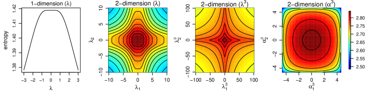
Figure 3: Plots of the entropy for different parametrizations with $C=I_{2}$.

In the remainder of this section, we discuss some applications where the lower bound can be computed in closed form or numerical integration can be performed efficiently. These simpler applications also present an opportunity to investigate how the different parametrizations alter the surface of the lower bound. Before that, we first explain how the accuracy of different approaches will be assessed.

3.3 Accuracy assessment

The objective in variational approximation is to maximize the lower bound ${\mathcal{L}}$, and a higher value of ${\mathcal{L}}$ is indicative of a better approximation closer in KL divergence to the true posterior. However, it is hard to quantify how significant an improvement of 0.1 in ${\mathcal{L}}$ is for instance. Following Faes et al. (2011), we assess the accuracy of $q(\theta)$ using the integrated absolute error by comparing it against a gold standard $q_{\text{GS}}(\theta)$ computed via numerical integration where plausible, or by using the kernel density estimate constructed using a sufficiently large number of MCMC samples. The integrated absolute error,

$$\text{IAE}(q)=\int|q(\theta)-q_{\text{GS}}(\theta)|d\theta,$$

is invariant to monotone transformations of $\theta$ and is a value between 0 and 2. Thus we can use as a discrepancy measure, $\text{Accuracy}(q)=1-\text{IAE}(q)/2$, which is expressed as a percentage in later applications. MCMC is performed using RStan, where 2 chains each of 50000 iterations are run in parallel and the first half is discarded as burn-in. The remaining 50000 draws are used to construct the kernel density estimate.

3.4 Normal sample

Let $\theta=(\theta_{1},\theta_{2})$ and consider the model for a normal sample,

$$y_{i}|\theta\sim{\text{N}}(\theta_{1},\exp(\theta_{2})),\quad 1\leq i\leq n,$$

with priors $\theta_{1}\sim{\text{N}}(0,\sigma_{0}^{2})$ and $\exp(\theta_{2})\sim{\text{IG}}(a_{0},b_{0})$ where $a_{0}=b_{0}=0.01$ and $\sigma_{0}^{2}=10^{4}$ (Ormerod, 2011). Applying Lemma 1,

$${\text{E}}_{q}\{\log p(y,\theta)\} =c_{*}-(a_{0}+n/2)\mu_{2}-(\Sigma_{11}+\mu_{1}^{2})/(2\sigma_{0}^{2})-M(b_{0}+T/2),$$

where $c_{*}=a_{0}\log b_{0}-\log\Gamma(a_{0})-\frac{1}{2}\log(\sigma_{0}^{2})-\frac{n+1}{2}\log(2\pi)$, $T=\sum_{i=1}^{n}(y_{i}-\tilde{\mu}_{1})^{2}+n\tilde{\Sigma}_{11}$, and $M$, $\tilde{\mu}$ and $\tilde{\Sigma}$ are as defined in Lemma 1 with $s=-e_{2}$. Derivation details are provided in the Supplement S2.

First, we consider a simplification where $\theta_{1}$ is fixed at 0 and $\theta=\theta_{2}$ only. The true posterior of $\theta$ then lies in the same family as the prior with the parameters $a_{0}$ and $b_{0}$ replaced by $a_{1}=a_{0}+n/2$ and $b_{1}=b_{0}+\sum_{i=1}^{n}y_{i}^{2}/2$ respectively. However, this problem is useful for investigating the behavior of the lower bound in the vicinity of $\lambda=0$. Following Ormerod (2011), we simulate $n=6$ observations from the model by setting $\exp(\theta_{2})=225$. Writing $C$ as $\sigma$, Figure 4 shows the profile lower bound for $\lambda$, ${\mathcal{L}}(\lambda)={\mathcal{L}}(\hat{\mu}(\lambda),\hat{\sigma}(\lambda),\lambda)$, where $\hat{\mu}$ and $\hat{\sigma}$ are the values that maximize ${\mathcal{L}}$ for any given $\lambda$. The leftmost plot is very similar to that of the profile log likelihood in Arellano-Valle and Azzalini (2008), which has a stationary point at $\lambda=0$ and a non-quadratic shape that increases the risk of getting stuck at $\lambda=0$ during optimization.

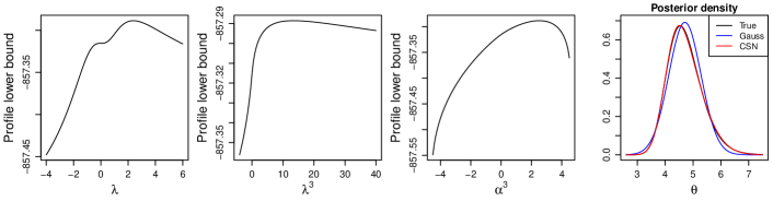
Figure 4: First three plots show the profile lower bound for $\lambda$, $\lambda^{3}$ and $\alpha^{3}$. Last plot shows true posterior density and the Gaussian and CSN variational approximations.

It demonstrates that simply using the “centered” parameters $\mu$ and $\sigma$ is insufficient in getting rid of the stationary point at $\lambda=0$, but replacing $\lambda$ by $\lambda^{3}$ or $\alpha^{3}$ achieves this goal. Among these two options, $\alpha^{3}$ yields a more pronounced mode that aids optimization. The last plot compares the true posterior density with the CSN (${\mathcal{L}}=-26.45$) and Gaussian (${\mathcal{L}}=-26.47$) variational approximations computed using optim in R. The CSN has a much higher accuracy of 99.0% compared to the Gaussian (92.6%).

Figure 5: Contour plots of true posterior density and variational approximations. For SN, results from two initializations are shown, capturing either the left or right tail.

Methods	Gaussian	SN (Left tail)	SN (Right tail)	CSN (Cholesky)	CSN (LU)
Lower bound	-29.75	-29.69	-29.69	-29.72	-29.64
Accuracy (%)	85.0	89.4	88.0	87.9	95.3

Table 1: Lower bounds and accuracies (%) of variational approximations.

Returning to the problem where both $\theta_{1}$ and $\theta_{2}$ are unknown, $n=6$ observations are simulated from the model by setting $\theta_{1}=100$ and $\exp(\theta_{2})=225$. Figure 5 compares contour plots of the true posterior with variational approximations computed using optim in R, while Table 1 shows the lower bound and accuracy. We estimate the normalizing constant of the true posterior by integrating out $\theta_{1}$ analytically and then integrating with respect to $\theta_{2}$ numerically. The skew and closed skew normals are more sensitive to initialization than the Gaussian and we report the best result for each method after trying different initializations. The Gaussian variational approximation is least accurate as it cannot accommodate any skewness. The skew normal can capture the left or right tail depending on the initialization but not both because it is bounded in only one direction. For the CSN subclass, the approximation does not have the correct orientation if $C$ is the Cholesky factor of $\Sigma$ as rotations cannot be performed but it still improves upon the Gaussian. The LU decomposition achieves the highest lower bound and accuracy of 95.3%, albeit at the cost of more unknown parameters. This example illustrates a case where parametrizing $C$ using the Cholesky factor is inadequate, while a full $d\times d$ matrix yields more flexibility leading to an improved variational approximation. Finally, we investigate the lower bound of CSN (LU) evaluated at $\mu=\hat{\mu}$, $L=\hat{C}$ and $U=I_{d}$ for different parametrizations of $\lambda$ in Figure 6, which is a useful way of initializing the variational parameters. For $\lambda$, the stationary point at zero can be observed. Again, it seems that $\alpha^{3}$ yields a quadratic-like surface that provides the greatest ease in optimization.

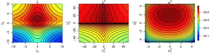
Figure 6: Evidence lower bound for CSN (LU) at $\mu=\hat{\mu}$, $L=\hat{C}$ and $U=I_{d}$ for different parametrizations of $\lambda$, where $(\hat{\mu},\hat{C})$ are optimal parameters for Gaussian approximation.

3.5 Poisson generalized linear model

Another application where ${\text{E}}_{q}\{\log p(y,\theta)\}$ can be computed analytically is the Poisson generalized linear model. Consider a dataset (Scotto et al., 1974) on the incidence of non-melanoma skin cancer by age group (15–24, …, 75–84, 84+) in Dallas-Fort Worth and Minneapolis-St. Paul, given in Table 6 of Gart (1979). Let $y_{i}\sim\text{Poisson}(\gamma_{i})$ be the number of skin cancer cases in group $i$ out of a population $T_{i}$, where the expected rate is modeled as $\log(\mu_{i}/T_{i})=x_{i}^{T}\theta$ for $i=1,\dots,n$ and $\log(T_{i})$ acts as an offset. The covariates $x_{i}$ are dummy variables for age group and town, such that $n=16$ and $d=9$. A normal prior ${\text{N}}(0,\sigma_{o}^{2}I_{d})$ is placed on $\theta$, where $\sigma_{0}=100$. Applying Lemma 1 again, we obtain

$${\text{E}}_{q}\{\log p(y,\theta)\}=y^{T}X\mu-\frac{\text{\rm tr}(\Sigma)+\mu^{T}\mu}{2\sigma_{0}^{2}}-2^{d}\sum_{i=1}^{n}T_{i}\exp\{\mu^{*T}x_{i}+x_{i}^{T}\Sigma^{*}x_{i}/2\}\Phi(D_{\alpha}C^{T}x_{i})+c_{*},$$

where $c_{*}=-\frac{d}{2}\log(2\pi\sigma_{o}^{2})+\sum_{i=1}^{n}\{y_{i}\log(T_{i})-\log(y_{i}!)\}$. Optimal parameters for the variational approximations are obtained using the BFGS algorithm via Optim in R. Table 2 shows that the Gaussian variational approximation has an accuracy of about 95% compared to MCMC for the marginal densities of all parameters except $\theta_{9}$, while the approximations incorporating skewness can attain an accuracy of close to 99%. This improvement in approximation of the marginal densities can also be observed in Figure 7. While the CSN (Cholesky and LU) attains a slightly higher lower bound than the SN indicating a mildly better approximation of the joint posterior, the differences are hardly distinguishable marginally. Examination of the bivariate MCMC draws do not indicate a need for a bounding line in each dimension, which may help to explain why SN performs as well as the CSN subclass.

	${\mathcal{L}}$	$\theta_{1}$	$\theta_{2}$	$\theta_{3}$	$\theta_{4}$	$\theta_{5}$	$\theta_{6}$	$\theta_{7}$	$\theta_{8}$	$\theta_{9}$
Gaussian	-115.027	94.9	95.5	95.2	94.9	94.9	94.9	95.0	95.4	99.3
SN	-115.011	98.7	98.6	98.6	98.7	98.6	98.6	98.7	98.6	99.3
CSN (Cholesky)	-115.009	98.6	98.9	98.7	98.7	98.6	98.6	98.7	98.7	99.4
CSN (LU)	-115.008	98.6	98.8	98.6	98.7	98.5	98.5	98.6	98.7	99.3

Table 2: Lower bounds and accuracies (%) of variational approximations.

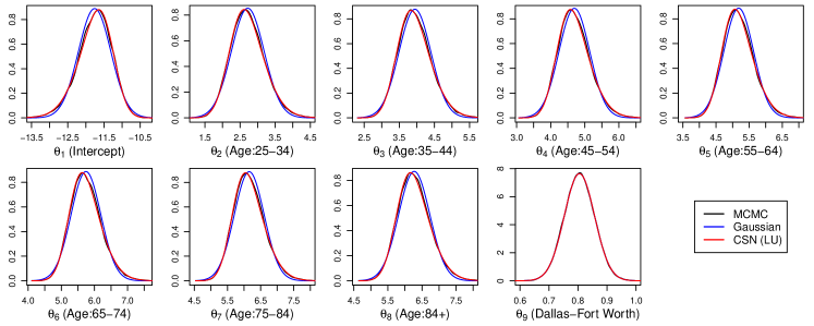
Figure 7: Contour plots of true posterior density and variational approximations. For SN, results from two initializations are shown, capturing either the left or right tail.

4 Stochastic variational inference for CSN subclass

For many models, the term ${\text{E}}_{q}\{\log p(y,\theta)\}$ is not analytically tractable. In such cases, we can maximize ${\mathcal{L}}$ with respect to the variational parameters $\eta$ using stochastic gradient ascent (Robbins and Monro, 1951), where an update

$$\eta_{t+1}=\eta_{t}+\rho_{t}\widehat{\nabla}_{\eta}{\mathcal{L}}(\eta_{t})$$

is performed at the $t$th iteration and $\widehat{\nabla}_{\eta}{\mathcal{L}}(\eta_{t})$ is an unbiased estimate of the true gradient $\nabla_{\eta}{\mathcal{L}}$ evaluated at $\eta_{t}$. This algorithm will converge to a local optimum if certain regularity conditions are obeyed and the stepsize $\rho_{t}$ satisfies $\sum_{t=1}^{\infty}\rho_{t}=\infty$ and $\sum_{t=1}^{\infty}\rho_{t}<\infty$ (Spall, 2003). Unbiased gradient estimates can be computed via the reparametrization trick (Kingma and Welling, 2014). Suppose $\theta=\mathcal{T}_{\eta}(z)$ where $\mathcal{T}_{\eta}(\cdot)$ is a differentiable function containing all information involving $\eta$, and it is easy to simulate from the density $p(z)$ of $z$ which is independent of $\eta$. Then

$$\nabla_{\eta}{\mathcal{L}}={\text{E}}_{p(z)}\{\nabla_{\eta}\theta\nabla_{\theta}h(\theta)\},$$

and an unbiased estimate is $\widehat{\nabla}_{\eta}{\mathcal{L}}=\nabla_{\eta}\theta\nabla_{\theta}h(\theta)$, where $\theta=\mathcal{T}_{\eta}(z)$ and $z$ is generated from $p(z)$. The score function method in (6) can also be used to obtain an unbiased estimate of $\nabla_{\eta}{\mathcal{L}}$. However, the marginal variance of gradients estimated using the reparametrization trick were shown to be smaller than the score function method for quadratic log likelihoods in variational Bayes (Xu et al., 2019). The reparametrization trick is widely applied in Gaussian variational approximation (Titsias and Lázaro-Gredilla, 2014). If $\theta\sim{\text{N}}(\mu,CC^{T})$, then $\theta=Cz+\mu$ where $z\sim{\text{N}}(0,I_{d})$. For our CSN subclass, we can use the stochastic representation in property (P7) to find $\nabla_{\eta}\theta$. As for $\nabla_{\theta}h(\theta)=\nabla_{\theta}\log p(y,\theta)-\nabla_{\theta}\log q(\theta)$, $\nabla_{\theta}\log p(y,\theta)$ is model dependent while

$$\nabla_{\theta}\log q(\theta) =C^{-T}D_{\tau}\{D_{\lambda}\zeta_{1}(D_{\lambda}v)-v\},$$

where $v=D_{\tau}C^{-1}(\theta-\mu)+b\delta$. If $C$ is the Cholesky factor, then $\eta=(\mu^{T},\lambda^{T},\text{\rm vech}(C)^{T})^{T}$, where $\text{\rm vech}(C)$ is the vectorization of lower triangular elements in $C$ columnwise from left to right. Let $w_{3}=\{\widetilde{w}_{1}-(1-b^{2})D_{\lambda}w_{2}\}\odot C^{T}\nabla_{\theta}h(\theta)$, where $\odot$ is the Hadamard product. Then

$$\widehat{\nabla}_{\eta}{\mathcal{L}}=\nabla_{\eta}\theta\nabla_{\theta}h(\theta)=\begin{bmatrix}\nabla_{\theta}h(\theta)^{T},&(D_{\kappa}^{3}w_{3})^{T},&\text{\rm vech}(\nabla_{\theta}h(\theta)z^{T})^{T}\end{bmatrix}^{T}.$$

On the other hand, if $C=LU$ where $L$ is a lower triangular matrix and $U$ is an upper triangular matrix with unit diagonal, then $\eta=(\mu^{T},\lambda^{T},\text{\rm vech}(L)^{T},\text{\rm vech}_{u}(U)^{T})^{T}$, where $\text{\rm vech}_{u}(\cdot)$ vectorizes elements above the diagonal columnwise from left to right. Then $\widehat{\nabla}_{\mu}{\mathcal{L}}$ and $\widehat{\nabla}_{\lambda}{\mathcal{L}}$ remain unchanged while

$$\widehat{\nabla}_{\text{\rm vech}(L)}{\mathcal{L}}=\text{\rm vech}(\nabla_{\theta}h(\theta)z^{T}U^{T}),\quad\text{and}\quad\widehat{\nabla}_{\text{\rm vech}_{u}(U)}{\mathcal{L}}=\text{\rm vech}_{u}(L^{T}\nabla_{\theta}h(\theta)z^{T}).$$

More details are given in the supplement S3. If $\alpha^{3}$ is used as parameter instead of $\lambda$, then

$$\widehat{\nabla}_{\alpha^{3}}{\mathcal{L}}=(\nabla_{\alpha^{3}}\lambda)\widehat{\nabla}_{\lambda}{\mathcal{L}}=\tfrac{1}{3}D_{\alpha}^{-2}D_{\kappa}^{-3}(D_{\kappa}^{3}w_{3})=\tfrac{1}{3}D_{\alpha}^{-2}w_{3}.$$

4.1 Natural gradients for CSN subclass

The steepest ascent direction is given by the (Euclidean) gradients derived previously when the distance between $\eta$s is measured using the Euclidean metric. However, as we are optimizing the lower bound ${\mathcal{L}}$ with respect to $\eta$ in a curved parameter space, the Euclidean metric may not be appropriate. When distance between densities is measured using KL divergence, the steepest ascent direction is given by the natural gradient (Amari, 2016), which premultiplies the Euclidean gradient with the Fisher information matrix, $\mathcal{I}_{\theta}(\eta)=-{\text{E}}_{q}\{\nabla_{\eta}^{2}\log q(\theta)\}$.

For the skew normal distribution, the Fisher information matrix is singular at $\lambda=0$ and involves expectations which are not analytically tractable (Arellano-Valle and Azzalini, 2008). These present difficulties in the derivation and use of natural gradients. Lin et al. (2019) overcame this problem and derived natural gradients updates for the skew normal using a minimal conditional exponential families representation, but their update of $\Sigma$ does not ensure positive definiteness. Here, we derive analytic natural gradients for a subclass of the closed skew normal which ensures positive definiteness by considering the Cholesky or LU decomposition, and the Fisher information of $q(\theta,w)$ defined in property (P7) instead. This is possible because

$${\mathcal{L}}=\int q(\theta)h(\theta)d\theta=\int\int q(\theta,w)h(\theta)d\theta dw,$$

and $q(\theta,w)$ shares the same parameters $\eta$ as $q(\theta)$. Hence we can imagine that we are optimizing ${\mathcal{L}}$ in the parameter space of $q(\theta,w)$, in which case the natural gradient is $\widetilde{\nabla}_{\eta}{\mathcal{L}}=\mathcal{I}_{\theta,w}(\eta)^{-1}\nabla_{\eta}{\mathcal{L}}$ instead of $\mathcal{I}_{\theta}(\eta)^{-1}\nabla_{\eta}{\mathcal{L}}$, where

$$\mathcal{I}_{\theta,w}(\eta) =-{\text{E}}_{q(\theta,w)}\{\nabla_{\eta}^{2}\log q(\theta,w)\}$$

$$=-{\text{E}}_{q(\theta)}\{\nabla_{\eta}^{2}\log q(\theta)\}-{\text{E}}_{q(\theta)}{\text{E}}_{q(w|\theta)}\{\nabla_{\eta}^{2}\log q(w|\theta)\}$$

$$=\mathcal{I}_{\theta}(\eta)+{\text{E}}_{q(\theta)}\{\mathcal{I}_{w|\theta}(\eta|\theta)\}.$$

The above relationship shows that $\mathcal{I}_{\theta,w}(\eta)$ is “more positive definite” than $\mathcal{I}_{\theta}(\eta)$ and hence it is useful to consider natural gradients based on $\mathcal{I}_{\theta,w}(\eta)$ when $\mathcal{I}_{\theta}(\eta)$ has singularities, although the progress in gradient ascent may be more conservative. From property (P7),

$$\log q(\theta,w) =\log q(\theta|w)+\log q(w)$$

$$=-d\log(2\pi)-\log|C|-\sum_{i=1}^{d}\log\kappa_{i}-\frac{w^{T}w}{2}-\frac{z^{T}D_{\kappa}^{-2}z}{2}-\frac{\widetilde{w}^{T}D_{\lambda}^{2}\widetilde{w}}{2}+z^{T}D_{\lambda}D_{\kappa}^{-1}\widetilde{w},$$

where $z=C^{-1}(\theta-\mu)$. If $C=LU$, then $\log|C|=\log|L|$ since $U$ has unit diagonal. The Fisher information $\mathcal{I}_{\theta,w}(\eta)$ is obtained by taking the negative expectation of $\nabla_{\eta}^{2}\log q(\theta,w)$, found using vector differential calculus (Magnus and Neudecker, 1980, 1999). The inverse can be found using block matrix inversion and we pre-multiply the Euclidean gradient $\nabla_{\eta}{\mathcal{L}}$ with $\mathcal{I}_{\theta,w}(\eta)^{-1}$ to obtain the natural gradient $\widetilde{\nabla}_{\eta}{\mathcal{L}}$. The results are presented in the next two Theorems and proofs are given in the Supplement S4.

First, we define some notation. For any square matrix $X$, let $X_{\ell}$ and $X_{u}$ be the lower and upper triangular matrices derived from $X$ respectively by replacing all elements above the diagonal by zeros, and all elements on and below the diagonal by zeros. For $s\in\mathbb{R}^{d(d+1)/2}$, define $\text{\rm vech}^{-1}(s)$ as a $d\times d$ lower triangular matrix filled with elements of $s$ columnwise from left to right. For $t\in\mathbb{R}^{d(d-1)/2}$, define $\text{\rm vech}_{u}^{-1}(t)$ as a $d\times d$ upper triangular matrix with zero diagonal filled with elements of $t$ columnwise from left to right. Let $K=\kappa^{2}{\bf 1}^{T}$.

Theorem 2.

For the variational density $q(\theta)$ in the CSN subclass in (4), if $C$ is the Cholesky factor of $\Sigma$ and $\eta=(\mu^{T},\lambda^{T},\text{\rm vech}(C)^{T})^{T}$, then the natural gradient is

$$\widetilde{\nabla}_{\eta}{\mathcal{L}}=\begin{bmatrix}(CD_{\kappa}^{2}C^{T})\nabla_{\mu}{\mathcal{L}}\\ \tfrac{1}{(1-b^{2})(2\kappa^{2}-\kappa^{4})}\odot\nabla_{\lambda}{\mathcal{L}}+\tfrac{\lambda}{2-\kappa^{2}}\odot\text{\rm diag}(A_{1})\\ \text{\rm vech}(CA_{1}),\end{bmatrix},$$

where $G=\{C^{T}\text{\rm vech}^{-1}(\nabla_{\text{\rm vech}(C)}{\mathcal{L}})\}_{\ell}$ and $A_{1}=\text{\rm diag}(\tfrac{\alpha\kappa}{2}\odot\nabla_{\lambda}{\mathcal{L}})+G\odot\{K-\text{\rm diag}(\tfrac{\kappa^{4}}{2})\}$.

Theorem 3.

For the variational density $q(\theta)$ in the CSN subclass in (4), if $C=LU$ where $L$ is a lower triangular matrix and $C$ is an unit diagonal upper triangular matrix, and $\eta=(\mu^{T},\lambda^{T},\text{\rm vech}(L)^{T},\text{\rm vech}_{u}(U)^{T})^{T}$, then the natural gradient is given by

$$\widetilde{\nabla}_{\mu}{\mathcal{L}} =(CD_{\kappa}^{2}C^{T})\nabla_{\mu}{\mathcal{L}},$$

$$\widetilde{\nabla}_{\lambda}{\mathcal{L}} =\tfrac{1}{(1-b^{2})(2\kappa^{2}-\kappa^{4})}\odot\nabla_{\lambda}{\mathcal{L}}+\tfrac{\lambda}{2-\kappa^{2}}\odot\text{\rm diag}(H),$$

$$\widetilde{\nabla}_{\text{\rm vech}(L)}{\mathcal{L}} =\text{\rm vech}(L{\mathcal{G}}_{\ell}),$$

$$\widetilde{\nabla}_{\text{\rm vech}_{u}(U)}{\mathcal{L}} =\text{\rm vech}_{u}[U\{K_{u}\odot(F-H^{T})\}+{\mathcal{G}}_{u}U],$$

where $a=\text{\rm vech}\{\text{\rm diag}(\frac{1}{2-\kappa^{2}})+(1/K)_{\ell}-(K_{u})^{T}\}$,

$$\begin{aligned} G&=\{L^{T}\text{\rm vech}^{-1}(\nabla_{\text{\rm vech}(L)}{\mathcal{L}})\}_{\ell},\\ F&=\{U^{T}\text{\rm vech}_{u}^{-1}(\nabla_{\text{\rm vech}_{u}(U)}{\mathcal{L}})\}_{u},\end{aligned}\quad\begin{aligned} H&=A_{2}\odot[U^{T}\{G-(U^{-T}FU^{T})_{\ell}\}U^{-T}\\ &\;+\text{\rm diag}(\tfrac{\lambda}{2-\kappa^{2}}\odot\nabla_{\lambda}{\mathcal{L}})-(K\odot F)^{T}],\end{aligned}\quad\begin{aligned} {\mathcal{G}}&=UHU^{-1},\\ A_{2}&=\text{\rm vech}^{-1}(1/a).\end{aligned}$$

When $\nabla_{\eta}{\mathcal{L}}$ is intractable, we can replace it in Theorems 2 and 3 by $\widehat{\nabla}_{\eta}{\mathcal{L}}$ to obtain unbiased estimates of the natural gradient. If we wish to parametrize in terms of $\alpha^{3}$ instead of $\lambda$, then from Tan (2022),

$$\widetilde{\nabla}_{\alpha^{3}}{\mathcal{L}}=(\nabla_{\lambda}\alpha^{3})^{T}\widetilde{\nabla}_{\lambda}{\mathcal{L}}=3D_{\alpha}^{2}D_{\kappa}^{3}\widetilde{\nabla}_{\lambda}{\mathcal{L}}.$$

5 Applications

This section investigates the performance of proposed methods using various statistical applications, including logistic regression, a survival model and the zero-inflated negative binomial model. In each application, an independent ${\text{N}}(0,\sigma_{0}^{2})$ prior is specified for each element in $\theta$, where $\sigma_{0}^{2}=100$. Details concerning the joint log-likelihood function $\log p(y,\theta)$ and corresponding gradient $\nabla_{\theta}\log p(y,\theta)$ are provided in the Supplement S5. We compare the performance of the closed skew normal variational approximations based on the Cholesky factorization (CSNC) and LU decomposition (CSNLU) using the Gaussian as a baseline. The CSNC and CSNLU algorithms are run for a budget of 50000 iterations, and they are initialized using the Gaussian variational approximation. The skewness parameter is initialized as ${\bf 1}$ or $-{\bf 1}$, and a useful strategy is to run the algorithm for 1000 iterations from each starting point and then continue with the run that has a higher average lower bound. Lower bound estimates are averaged over every 1000 iterations due to the large amount of noise that is present. The results returned by the $\alpha^{3}$ and $\lambda$ parametrizations are often similar given a reasonably good starting point and hence we only report results of using $\alpha^{3}$. However, $\lambda$ has a high likelihood of getting stuck at zero if the starting point is poor, as we will illustrate later. We use Adam (Kingma and Ba, 2015) to compute the stepsize when using Euclidean gradients and a constant stepsize of 0.001 for natural gradients. This is because Adam is a sign-based variance adapted approach (Balles and Hennig, 2018), which is very useful for unscaled Euclidean gradients but it does not work well with natural gradients as the scaling performed by the Fisher information is largely neglected Tan (2022). Codes are written in R and Julia (version 1.8.4), and are available as supplementary material.

5.1 Logistic regression model

Figure 8: Contour plots of true posterior density and variational approximations for bioassay data.

Consider the bioassay data by Racine et al. (1986), where a dose ($x_{i}$) of chemical compound is administered to $n_{i}$ animals in each of $i=1,\dots,n$ trials, with $n=4$. The number of deaths $y_{i}$ in each trial is modeled independently as $y_{i}\sim\text{Binomial}(n_{i},p_{i})$, and a logistic regression model, $\text{\rm logit}(p_{i})=\beta_{0}+\beta_{1}x_{i}$, is used so that $\theta=(\beta_{0},\beta_{1})^{T}$. The normalizing constant of the true posterior density is estimated using Monte Carlo integration based on one billion samples. From Figure 8, the Gaussian, CSNC and CSNLU variational approximations have accuracies of around 85%, 92% and 95% respectively. The orientation of the posterior approximation of CSNC does not match the true posterior well, likely due to its inability to perform rotations. When the algorithms are initialized using $\lambda={\bf 1}$, the difference between the $\lambda$ and $\alpha^{3}$ parametrizations is indistinguishable, but significant improvements in the $\alpha^{3}$ parametrization can be observed when initialized using $\lambda=-{\bf 1}$. The first two plots of Figure 9 show that $\lambda$ converges slowly and is stuck at zero when parametrized directly using $\lambda$. However, when parametrized using $\alpha^{3}$, the iterates are able to escape the stationary point at zero and converge to a better local mode. The last two plots show the lower bounds when a constant stepsize of 0.001 is used and natural gradients consistently yield higher lower bounds. A major advantage of natural gradients is that they are scaled according to the curvature of the parameter space, unlike Euclidean gradients which enables the use of a small constant stepsize. While this approach still works with Euclidean gradients in this low-dimensional problem, a parameter-wise adaptive stepsize is usually necessary for algorithms based on Euclidean gradients to converge.

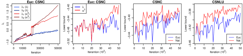
Figure 9: Bioassay data. First two plots show the trace of $\lambda$ and lower bound from the CSNC algorithm using either the $\lambda$ or $\alpha^{3}$ parametrizations. Last two plots show the lower bounds based on a constant stepsize of 0.001 for the CSNC and CSNLU algorithms.

Figure 10: Contour plots of true posterior density and variational approximations for O-ring data.

Now, consider the logistic regression model for binary responses, where $y_{i}\sim\text{Bernoulli}(p_{i})$ independently and $\text{\rm logit}(p_{i})=x_{i}^{T}\theta$ for $i=1,\dots,n$, where $\theta\in\mathbb{R}^{d}$ and $x_{i}\in\mathbb{R}^{d}$ represent the regression coefficients and covariates for the $i$th response respectively. We fit this model to the O-ring data in the GLMsData R package, where $y_{i}$ is an indicator for whether any O-rings were damaged for $n=23$ space shuttle launches and $x_{i}$ is the ambient air temperature (in degrees Fahrenheit) scaled to have mean zero and one standard deviation. For this low-dimensional problem, the normalizing constant of the posterior density is also estimated using Monte Carlo based on 1 billion samples. From Figure 10, the CSN approximations achieve a higher accuracy of about 96% compared to 89% for the Gaussian. For the CSNLU algorithm, $\lambda$ converges to $(-1.6,-2.6)$. If initialized using $\lambda={\bf 1}$, Figure 11 shows that the $\lambda$ parametrization is again stuck at zero while the $\alpha^{3}$ parametrization, being more resilient against initialization, is able to escape this stationary point and converge to $(-1.6,-2.6)$.

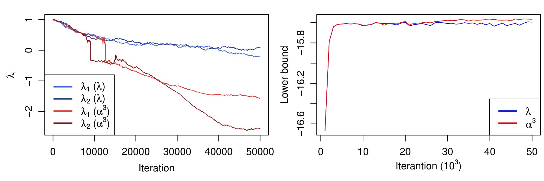
Figure 11: O-ring data. Trace of $\lambda$ and lower bound from the CSNLU algorithm (based on Euclidean gradients) using either the $\lambda$ and $\alpha^{3}$ parametrizations.

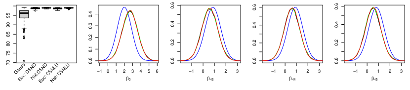
Figure 12: German credit data. Left: Boxplot shows the accuracies of marginal densities estimates compared with MCMC. Next four plots show marginal density estimates (MCMC: black, CSNC: green, CSNLU: red) of coefficients whose Gaussian approximation (blue) is less than 85%.

Lastly, we consider the German credit data from the UCI Machine Learning Repository, which contain the attributes of $n=1000$ people classified as having good or bad credit risks. All quantitative predictors are scaled to have mean zero and one standard deviation while qualitative predictors are coded using dummy variables. Due to the high-dimensionality of this data, we only compare the accuracies of marginal densities instead of the full joint posterior. For the CSN, kernel density estimates are computed based on 50,000 samples as it is challenging to evaluate $\Phi_{d}$ for $d=49$, while the ground truth is taken to be kernel density estimates constructed from MCMC samples. The boxplot in Figure 12 shows that the CSN improves significantly upon the Gaussian variational approximation with a minimum accuracy of 97.2% overall, while the use of natural gradients improve the minimum accuracy further to 98.2%. This figure also shows the marginal densities of the four coefficients where the Gaussian approximation has an accuracy less that 85%. The CSN corrects very well for the skewness in each case and is almost indistinguishable from MCMC.

5.2 Zero-inflated negative binomial model

The zero-inflated negative binomial model is used to model counts with excessive zeros while allowing for overdispersion. We fit this model to a dataset on the number of fish ($y_{i}$) caught by visitor $i$ at a national park on a particular day for $i=1,\dots,n$, where $n=250$ (https://www.stata-press.com/data/r18/fish.dta). An observation $y_{i}$ is 0 with probability $\varphi_{i}$, or is generated from a negative binomial distribution with probability $1-\varphi_{i}$. The pdf of the negative binomial distribution with parameters $\alpha$ and $\mu_{i}$ is

$$p(y_{i})=\frac{\frac{1}{\alpha}^{1/\alpha}\Gamma(y_{i}+\frac{1}{\alpha})\mu_{i}^{y_{i}}}{y_{i}!\Gamma(\frac{1}{\alpha})(\mu_{i}+\frac{1}{\alpha})^{y_{1}+1/\alpha}},$$

which is obtained by integrating out $\tau_{i}$ from the hierarchical model, $y_{i}|\tau_{i}\sim\text{Poisson}(\mu_{i}\tau_{i})$ and $\tau_{i}\sim\text{Gamma}(\frac{1}{\alpha},\frac{1}{\alpha})$. The response $\mu_{i}$ is modeled as $\log\mu_{i}=x_{i}^{T}\beta$, where $x_{i}$ includes an intercept, an indicator for use of live bait (livebait) and number of accompanying persons (persons). The probability $\varphi_{i}$ (that the visitor did not fish) is modeled as $\text{\rm logit}(\varphi_{i})=z_{i}^{T}\gamma$, where the covariates in $z_{i}$ include an intercept, number of accompanying children (child) and an indicator for camping (camper). Thus $\theta=(\beta^{T},\gamma^{T},\log\alpha)^{T}$ and $d=7$.

	${\mathcal{L}}$	$\beta_{0}$	$\beta_{1}$	$\beta_{2}$	$\gamma_{0}$	$\gamma_{1}$	$\gamma_{2}$	$\log\alpha$
Gaussian	-425.80	99.0	99.1	99.4	67.4	65.5	68.1	95.0
Euc: CSNC	-425.38	98.9	98.8	98.3	82.0	81.0	76.4	96.5
Nat: CSNC	-425.27	99.0	98.8	98.8	83.9	83.2	78.1	96.9
Euc: CSNLU	-425.52	98.9	99.0	98.7	85.1	84.8	85.5	95.6
Nat: CSNLU	-425.22	99.0	99.1	99.2	84.7	85.1	85.2	96.6

Table 3: Lower bound and accuracies of marginal densities for fish data.

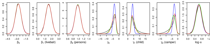
Figure 13: Marginal density estimates (MCMC: black, Gaussian:blue, CSNC: green, CSNLU: red) of coefficients for fish data.

From Table 3, the accuracy of the marginal density estimates for the Gaussian variational approximation is very high for $\beta$ ($\sim$99%) but is quite low for $\gamma$ ($\sim$67%) as its posteriors are highly asymmetrical. From Figure 13, the CSN improves on the Gaussian greatly but is also unable to capture all of the skewness. CSNLU ($\sim$85%) does better than than CSNC ($\sim$83%) and in each case, the use of natural gradients helps in improving the accuracy especially for CSNC. Figure 14 shows that the lower bounds based on natural gradients are consistently higher than that based on Euclidean gradients when a constant stepsize of 0.0002 is used. While a larger stepsize such as 0.001 can be used with natural gradients, the algorithms based on Euclidean gradients will diverge. The possibility of using a larger stepsize is another advantage of natural gradients. Lastly, Figure 15 shows the bivariate marginal posterior plot of $(\gamma_{1},\log\alpha)$, which is of a highly irregular shape. In higher dimensions, the accuracies of the variational approximations are likely to be lower than in one dimension and the differences among approaches are also magnified. The Gaussian is clearly inadequate in this setting while the CSNC and CSNLU are able to capture the skewness in the tail much more accurately albeit with limitations as well.

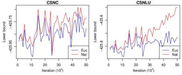
Figure 14: Fish data. Lower bounds based on a constant stepsize of 0.0002 for the CSNC and CSNLU algorithms.

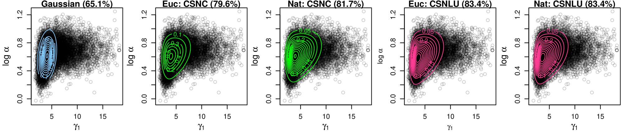
Figure 15: Fish data. Contour plots of variational approximations are superimposed on 10000 randomly selected MCMC samples.

5.3 Survival model

We consider a dataset for analyzing the effects of a hip-protection device, age and sex, on the risk of hip fractures in $n=148$ patients (https://www.stata-press.com/data/r18/hip3.dta). Each patient is observed up to a time $t_{i}$ at which an indicator $d_{i}$ for whether fracture occurs is recorded. For the Weibull proportional hazards model, the hazard function is $h(t_{i})=\rho_{i}t_{i}^{\rho_{i}-1}\exp(x_{i}^{T}\beta)$ for $i=1,\dots,n$, and the survival function is $S(t_{i})=\exp\{-\exp(x_{i}^{T}\beta)t_{i}^{\rho_{i}}\}$, where $\rho_{i}>0$. The covariates $x_{i}$ includes an intercept, an indicator for the use of hip-protection device (protect) and age. The hazard curves for men and women are assumed to be different in shape and the ancillary variable $\rho_{i}$ is modeled as $\log\rho_{i}=z_{i}^{T}\gamma$ where $z_{i}$ includes an intercept and sex to account for this difference. The variable age is standardized to have mean 0 and standard deviation of 1. Thus $\theta=(\beta^{T},\gamma^{T})^{T}$ and $d=5$.

	${\mathcal{L}}$	$\beta_{0}$	$\beta_{1}$	$\beta_{2}$	$\gamma_{0}$	$\gamma_{1}$
Gaussian	-165.22	95.3	99.1	99.0	95.1	90.5
Euc: CSNC	-165.11	96.0	98.7	98.7	95.5	97.6
Nat: CSNC	-165.10	96.3	98.8	98.9	94.4	97.2
Euc: CSNLU	-165.07	98.1	98.5	98.9	99.1	97.9
Nat: CSNLU	-165.06	97.8	98.6	98.9	97.7	98.2

Table 4: Lower bound and accuracies of marginal densities for hip data.

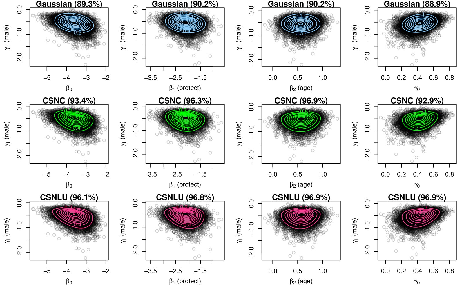
Figure 16: Hip data. Contour plots of variational approximations are superimposed on 10000 randomly selected MCMC samples.

From Table 4, the Gaussian variational approximation of the marginal density is highly accurate for the coefficients $\beta_{1}$ and $\beta_{2}$, reasonably good for $\beta_{0}$ and $\gamma_{0}$ and a little weaker for $\gamma_{1}$. The CSN is able to improve on the Gaussian for $\beta_{0}$ and $\gamma_{0}$, and especially $\gamma_{1}$. CSNLU being more flexible than CSNC is often able to provide improved accuracies, and this is also reflected in the bivariate marginal posterior plots in Figure 16. Finally, Figure 17 shows that when the CSNC algorithm is initialized from $\lambda={\bf 1}$, the iterates are again unable to traverse past the stationary point at zero while the $\alpha^{3}$ parametrization is able to overcome this problem and attain a much higher lower bound.

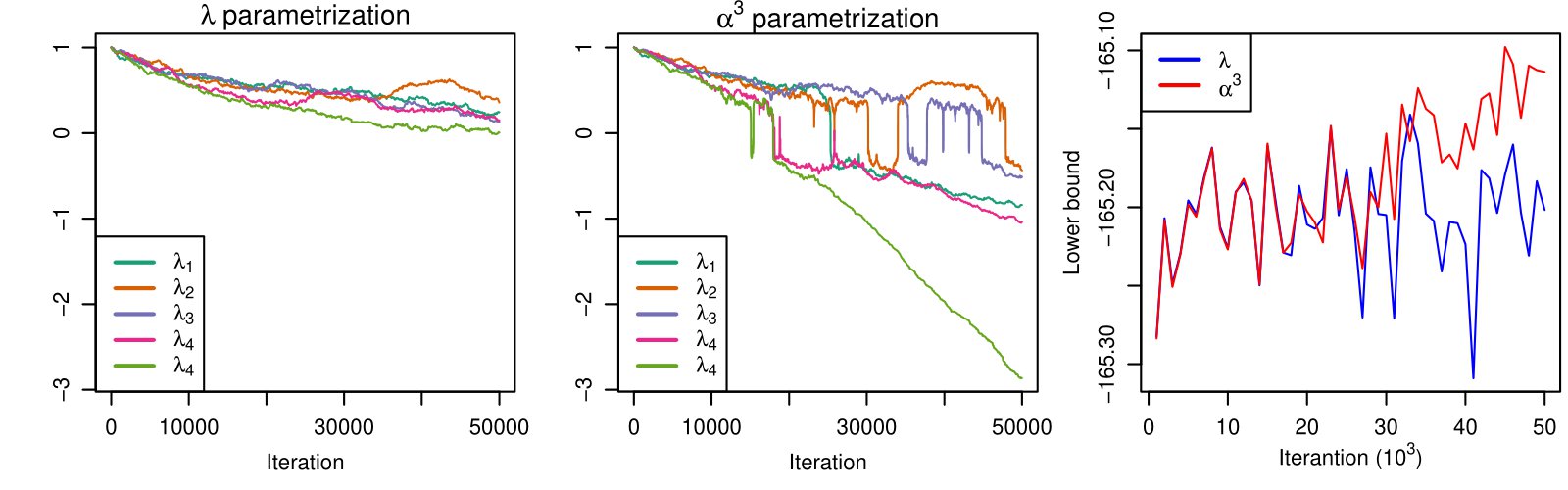
Figure 17: Hip data. Trace of $\lambda$ and lower bound from CSNC algorithm (based on Euclidean gradients) using either the $\lambda$ and $\alpha^{3}$ parametrizations.

6 Conclusion

In this article, we introduce a subclass of the closed skew normal as an alternative to Gaussian variational approximation that is able to accommodate skewness and is reasonably flexible in that a bounding line is permitted in each dimension unlike the original skew normal. This subclass is constructed using affine transformations and we highlight the limitations instilled by constraining the linear map to be a lower triangular matrix. A LU decomposition is proposed for the linear map when it is a full matrix to ensure ease in inversion during optimization. For the original skew normal, the presence of a stationary point when the skewness is zero is known to create issues in maximum likelihood estimation. We prove that such a stationary point similarly exists in the maximization of the evidence lower bound in variational inference, which creates problems in stochastic gradient ascent algorithms. We also demonstrate that parametrizing in terms of $\alpha^{3}$ is effective in resolving these issues. Finally, we develop analytic natural gradients for maximizing the lower bound using stochastic gradient ascent by considering the augmentation $q(\theta,w)$ instead of $q(\theta)$, that also ensures positive definiteness by using the Cholesky factorization or LU decomposition. The performance of proposed methods is investigated using a variety of statistical applications.

Supplementary Material

S1 Proof of Lemma 1

First, we present and prove Lemma S1.

Lemma S1.

Let $q(\theta)$ and $\tilde{q}(\theta)$ be the pdfs of ${\text{CSN}}_{d,q}(\mu,\Sigma,D,\nu,\Delta)$ and ${\text{CSN}}_{d,q}(\mu+\Sigma s,\Sigma,D,\nu-D\Sigma s,\Delta)$ respectively. Then

1. $\exp(s^{T}\theta)\phi_{d}(\theta|\mu,\Sigma)=\exp(\mu^{T}s+s^{T}\Sigma s/2)\phi_{d}(\theta|\mu+\Sigma s,\Sigma)$,

2. $\exp(s^{T}\theta)q(\theta)=\exp(\mu^{T}s+s^{T}\Sigma s/2)\tilde{q}(\theta)\dfrac{\Phi_{q}(0|\nu-D\Sigma s,\Delta+D\Sigma D^{T})}{\Phi_{q}(0|\nu,\Delta+D\Sigma D^{T})}$.

Proof.

For (i),

$$\exp(s^{T}\theta)\phi_{d}(\theta|\mu,\Sigma) =(2\pi)^{-d/2}|\Sigma|^{-1/2}\exp\big{[}-\tfrac{1}{2}\{\theta^{T}\Sigma^{-1}\theta-2\theta^{T}\Sigma^{-1}(\mu+\Sigma s)+\mu^{T}\Sigma^{-1}\mu\}\big{]}$$

$$=\phi_{d}(\theta|\mu+\Sigma s,\Sigma)\exp(\mu^{T}s+s^{T}\Sigma s/2).$$

For (ii), using the result in (i) we have

$$\exp(s^{T}\theta)q(\theta) =\exp(\mu^{T}s+s^{T}\Sigma s/2)\phi_{d}(\theta|\mu+\Sigma s,\Sigma)\frac{\Phi_{q}(D(\theta-\mu)|\nu,\Delta)}{\Phi_{q}(0|\nu,\Delta+D\Sigma D^{T})}$$

$$=\exp(\mu^{T}s+s^{T}\Sigma s/2)\tilde{q}(\theta)\frac{\Phi_{q}(0|\nu-D\Sigma s,\Delta+D\Sigma D^{T})}{\Phi_{q}(D(\theta-\mu-\Sigma s)|\nu-D\Sigma s,\Delta)}\frac{\Phi_{q}(D(\theta-\mu)|\nu,\Delta)}{\Phi_{q}(0|\nu,\Delta+D\Sigma D^{T})}$$

$$=\exp(\mu^{T}s+s^{T}\Sigma s/2)\tilde{q}(\theta)\dfrac{\Phi_{q}(0|\nu-D\Sigma s,\Delta+D\Sigma D^{T})}{\Phi_{q}(0|\nu,\Delta+D\Sigma D^{T})}.$$

∎

The result in Lemma 1 follows directly from Lemma S1(ii) by replacing $\mu$ by $\mu^{*}$, $\Sigma$ by $\Sigma^{*}$, $D$ by $D^{*}$ and setting $\nu=0$ and $\Delta=I_{d}$. Note that $\Phi_{d}(0|-D_{\lambda}D_{\tau}^{-1}C^{T}s,I_{d}+D_{\lambda}^{2})=\Phi(D_{\alpha}C^{T}s)$. The moment generating function of $\tilde{q}(\theta)$ is

$$M(t)=\frac{\Phi_{d}(D_{\alpha}C^{T}(t+s))}{\Phi(D_{\alpha}C^{T}s)}\exp\{t^{T}(\mu^{*}+\Sigma^{*}s)+t^{T}\Sigma^{*}t/2\},$$

and the log cumulant function is

$$K(t)=\log M(t)=\sum_{j=1}^{d}\log\Phi(\alpha_{j}C_{\cdot j}^{T}(t+s))+t^{T}(\mu^{*}+\Sigma^{*}s)+\frac{t^{T}\Sigma^{*}t}{2}+\text{constant}.$$

Substituting $t=0$ in the expressions below yields the mean and covariance of $\tilde{q}(\theta)$:

$$\nabla_{t}K(t) =\sum_{j=1}^{d}\zeta_{1}(\alpha_{j}C_{\cdot j}^{T}(t+s))\alpha_{j}C_{\cdot j}+\mu^{*}+\Sigma^{*}s+\Sigma^{*}t,$$

$$\nabla_{t}^{2}K(t) =\sum_{j=1}^{d}\zeta_{2}(\alpha_{j}C_{\cdot j}^{T}(t+s))\alpha_{j}^{2}C_{\cdot j}C_{\cdot j}^{T}+\Sigma^{*}.$$

S2 Normal sample

The induced prior for $\theta_{2}$ is $p(\theta_{2})={b_{0}}^{a_{0}}\exp\{-a_{0}\theta_{2}-b_{0}\exp(-\theta_{2})\}/\Gamma(a_{0})$ and

$$\log p(y,\theta)=c_{*}-\left(a_{0}+n/2\right)\theta_{2}-\exp(-\theta_{2})\left(b_{0}+\sum\nolimits_{i=1}^{n}(y_{i}-\theta_{1})^{2}/2\right)-\theta_{1}^{2}/(2\sigma_{0}^{2}),$$

From Lemma 1, taking $s$ as $-e_{2}$,

$$\exp(-e_{2}^{T}\theta)q(\theta)=2^{d}\Phi_{d}(-D_{\alpha}C^{T}e_{2})\exp(-e_{2}^{T}\mu^{*}+e_{2}^{T}\Sigma^{*}e_{2}/2)\tilde{q}(\theta)=M\tilde{q}(\theta).$$

Using this result and taking expectations,

$${\text{E}}_{q}\{\log p(y,\theta)\} =c_{*}-\left(\frac{n}{2}+a_{0}\right){\text{E}}_{q}(\theta_{2})-\int\underbrace{\exp(-\theta_{2})q(\theta)}_{M\tilde{q}(\theta)}\left(b_{0}+\frac{\sum_{i=1}^{n}(y_{i}-\theta_{1})^{2}}{2}\right)d\theta-\frac{{\text{E}}_{q}(\theta_{1}^{2})}{2\sigma_{0}^{2}}$$

$$=c_{*}-\left(\frac{n}{2}+a_{0}\right)\mu_{2}-M\left(b_{0}+\frac{n\tilde{\Sigma}_{11}+\sum_{i=1}^{n}(y_{i}-\tilde{\mu}_{1})^{2}}{2}\right)-\frac{e_{1}^{T}(CC^{T}+\mu\mu^{T})e_{1}}{2\sigma_{0}^{2}}.$$

In the univariate case,

$${\text{E}}_{q}\{\log p(y,\theta)\}=a_{0}\log b_{0}-\log\Gamma(a_{0})-\frac{n}{2}\log(2\pi)-(a_{0}+n/2)\mu-MT,$$

where $M=2\Phi(-\alpha\sigma)\exp(\sigma^{2}\tau^{2}/2-\mu+b\sigma\alpha)$, $T=b_{0}+\sum_{i=1}^{n}y_{i}^{2}/2$. The lower bound can be written as a function of $(\sigma,\lambda)$ only,

$${\mathcal{L}}(\sigma,\lambda)=a_{0}\log b_{0}-\log\Gamma(a_{0})-\frac{n}{2}\log(2\pi)-(a_{0}+n/2)\{f(\sigma,\lambda)+1\}+H_{q}.$$

since ${\mathcal{L}}$ is maximized at $\mu=f(\sigma,\lambda)=\sigma^{2}\tau^{2}/2+b\sigma\alpha-\log(a_{0}+n/2)+\log\{2T\Phi(-\sigma\alpha)\}$.

To find the normalization constant of the posterior density in the bivariate case, we first integrate $p(y,\theta)$ with respect to $\theta_{1}$. The integral with respect to only $\theta_{2}$ can then be evaluated numerically.

$$p(y) =\int p(y,\theta)d\theta$$

$$=\int\frac{b_{0}^{a_{0}}}{\Gamma(a_{0})}{\rm e}^{-a_{0}\theta_{2}-b_{0}\exp(-\theta_{2})}\cdot\frac{1}{\sqrt{2\pi\sigma_{0}^{2}}}{\rm e}^{-\theta_{1}^{2}/(2\sigma_{0}^{2})}\prod_{i=1}^{n}\frac{1}{\sqrt{2\pi}{\rm e}^{\theta_{2}/2}}{\rm e}^{-(y_{i}-\theta_{1})^{2}/(2{\rm e}^{\theta_{2}})}d\theta_{1}d\theta_{2}$$

$$=\int\frac{b_{0}^{a_{0}}\exp\{-(a_{0}+n/2)\theta_{2}-(b_{0}+\sum_{i=1}^{n}y_{i}^{2}/2)\exp(-\theta_{2})\}}{\Gamma(a_{0})(2\pi)^{(n+1)/2}\sqrt{\sigma_{0}^{2}}}\int{\rm e}^{-\frac{(\theta_{1}-m)^{2}}{2v}+\frac{m^{2}}{2v}}d\theta_{1}d\theta_{2}$$

$$=\int\frac{b_{0}^{a_{0}}\exp\{m^{2}/(2v)-(a_{0}+n/2)\theta_{2}-(b_{0}+\sum_{i=1}^{n}y_{i}^{2}/2)\exp(-\theta_{2})\}\sqrt{v}}{\Gamma(a_{0})(2\pi)^{n/2}\sqrt{\sigma_{0}^{2}}}d\theta_{2},$$

where $v=\{n\exp(-\theta_{2})+\sigma_{0}^{-2}\}^{-1}$, $m=vn\bar{y}\exp(-\theta_{2})$ and $\bar{y}=\sum_{i=1}^{n}y_{i}/n$.

S3 Reparametrization trick gradients

If $C$ is the Cholesky factor, then

$$\nabla_{\eta}\theta=\begin{bmatrix}\nabla_{\mu}\theta\\ \nabla_{\lambda}\theta\\ \nabla_{\text{\rm vech}(C)}\theta\end{bmatrix}=\begin{bmatrix}I_{d}\\ \text{\rm diag}\{\widetilde{w}_{1}-(1-b^{2})D_{\lambda}w_{2}\}D_{\kappa}^{3}C^{T}\\ \mathsf{E}_{\ell}(z\otimes I)\end{bmatrix},$$

On the other hand, if $C=LU$, then

$$\nabla_{\eta}\theta=\begin{bmatrix}\nabla_{\mu}\theta\\ \nabla_{\lambda}\theta\\ \nabla_{\text{\rm vech}(L)}\theta\\ \nabla_{\text{\rm vech}_{u}(U)}\theta\end{bmatrix}=\begin{bmatrix}I_{d}\\ \text{\rm diag}\{\widetilde{w}_{1}-(1-b^{2})D_{\lambda}w_{2}\}D_{\kappa}^{3}C^{T}\\ \mathsf{E}_{\ell}(Uz\otimes I)\\ \mathsf{E}_{u}(z\otimes L^{T})\end{bmatrix}.$$

S4 Natural gradients

First, we define some notation. Let $\mathsf{E}_{\ell}$, $\mathsf{E}_{u}$ and $\mathsf{E}_{d}$ denote elimination matrices such that $\mathsf{E}_{\ell}\text{\rm vec}(X)=\text{\rm vech}(X)$, $\mathsf{E}_{u}\text{\rm vec}(X)=\text{\rm vech}_{u}(X)$ and $\mathsf{E}_{d}\text{\rm vec}(X)=\text{\rm diag}(X)$. Conversely, $\mathsf{E}_{\ell}^{T}\text{\rm vech}(X)=\text{\rm vec}(X_{\ell})$, $\mathsf{E}_{u}^{T}\text{\rm vech}_{u}(X)=\text{\rm vec}(X_{u})$ and $\mathsf{E}_{d}^{T}\text{\rm diag}(X)=\text{\rm vec}\{\text{\rm dg}(X)\}$, where $\text{\rm dg}(X)$ is a diagonal matrix derived from $X$ by setting all non-diagonal elements to zero. Let $\mathsf{K}$ be the commutation matrix such that $\mathsf{K}\text{\rm vec}(X)=\text{\rm vec}(X^{T})$. We use $\otimes$ to denote the Kronecker product.

Let $\ell=\log q(\theta,w)$. For taking expectations, note that ${\text{E}}(z)=0$, ${\text{E}}(zz^{T})=I_{d}$, ${\text{E}}(\widetilde{w})=0$, ${\text{E}}(\widetilde{w}\widetilde{w}^{T})=(1-b^{2})I_{d}$, ${\text{E}}(z|w)=D_{\alpha}\widetilde{w}$, ${\text{E}}(z\widetilde{w}^{T})=(1-b^{2})D_{\alpha}$ and

$${\text{E}}[\nabla_{\mu}\ell z^{T}]=C^{-T}\{D_{\kappa}^{-2}-(1-b^{2})D_{\kappa}^{-1}D_{\lambda}D_{\alpha}\}=C^{-T}.$$

S4.1 Cholesky factorization (Proof of Theorem 1)

If $C$ is the Cholesky factor, the first order derivatives are

$$\nabla_{\mu}\ell =C^{-T}D_{\kappa}^{-1}\{D_{\kappa}^{-1}z-D_{\lambda}\widetilde{w}\},$$

$$\nabla_{\lambda}\ell =(1-b^{2})(\alpha\odot\kappa)-D_{\lambda}\{(1-b^{2})z^{2}+\widetilde{w}^{2}\}+\text{\rm diag}(2/\kappa-\kappa)(z\odot\widetilde{w}),$$

$$\nabla_{\text{\rm vech}(C)}\ell =\text{\rm vech}\{(\nabla_{\mu}\ell)z^{T}-C^{-T}\}.$$

The second order derivatives are

$$\nabla_{\mu}^{2}\ell =-C^{-T}D_{\kappa}^{-2}C^{-1},$$

$$\nabla_{\mu,\lambda}^{2}\ell =C^{-T}\text{\rm diag}\{2(1-b^{2})(\lambda\odot z)-(2/\kappa-\kappa)\odot\widetilde{w}\},$$

$$\nabla_{\text{\rm vech}(C),\mu}^{2}\ell =\mathsf{E}_{\ell}\{(z\otimes\nabla_{\mu}^{2}\ell)-(C^{-1}\otimes\nabla_{\mu}\ell)\},$$

$$\nabla_{\lambda}^{2}\ell =(1-b^{2})\text{\rm diag}\{2\kappa^{4}-\kappa^{2}+(2\alpha+\alpha\kappa^{2})\odot z\odot\widetilde{w}-z^{2}\}-\text{\rm diag}(\widetilde{w}^{2}),$$

$$\nabla_{\text{\rm vech}(C)}^{2}\ell =\mathsf{E}_{\ell}[(zz^{T}\otimes\nabla_{\mu}^{2}\ell)+\{(C^{-1}\otimes C^{-T})-(C^{-1}\otimes(\nabla_{\mu}\ell)z^{T})-(z(\nabla_{\mu}\ell)^{T}\otimes C^{-T})\}\mathsf{K}]\mathsf{E}_{\ell}^{T},$$

$$\nabla_{\text{\rm vech}(C),\lambda}^{2}\ell =\mathsf{E}_{\ell}(z\otimes\nabla_{\mu,\lambda}^{2}\ell).$$

Taking expectations, ${\text{E}}[\nabla_{\mu,\lambda}^{2}\ell]=0$, ${\text{E}}[\nabla_{\mu,\text{\rm vech}(C)}^{2}\ell]=0$,

$${\text{E}}[\nabla_{\lambda}^{2}\ell] =-(1-b^{2})\text{\rm diag}(2\kappa^{2}-\kappa^{4}),$$

$${\text{E}}[\nabla_{\text{\rm vech}(C)}^{2}\ell] =-\mathsf{E}_{\ell}\{(C^{-1}\otimes C^{-T})\mathsf{K}+(I_{d}\otimes C^{-T}D_{\kappa}^{-2}C^{-1})\}\mathsf{E}_{\ell}^{T},$$

$${\text{E}}[\nabla_{\text{\rm vech}(C),\lambda}^{2}\ell] =(1-b^{2})\mathsf{E}_{\ell}(I\otimes C^{-T})\mathsf{E}_{d}^{T}\text{\rm diag}(\alpha\kappa).$$

Note that

$$\mathcal{I}_{33} =\mathsf{E}_{\ell}\{\mathsf{K}(C^{-T}\otimes C^{-1})+(I_{d}\otimes C^{-T}D_{\kappa}^{-2}C^{-1})\}\mathsf{E}_{\ell}^{T}$$

$$=\mathsf{E}_{\ell}\{\mathsf{K}(C^{-T}\otimes I_{d})(I_{d}\otimes C^{-1})+(I_{d}\otimes C^{-T})(I_{d}\otimes D_{\kappa}^{-2})(I_{d}\otimes C^{-1})\}\mathsf{E}_{\ell}^{T}$$

$$=\mathsf{E}_{\ell}(I_{d}\otimes C^{-T})(\mathsf{K}+I_{d}\otimes D_{\kappa}^{-2})(I_{d}\otimes C^{-1})\mathsf{E}_{\ell}^{T}.$$

Thus we obtain the Fisher information matrix of $q(\theta,w)$, which is given by

$$\mathcal{I}_{\theta,w}(\eta)=\begin{bmatrix}(CD_{\kappa}^{2}C^{T})^{-1}&0&0\\ 0&\mathcal{I}_{22}&\mathcal{I}_{32}^{T}\\ 0&\mathcal{I}_{32}&\mathcal{I}_{33}\end{bmatrix},\quad\begin{aligned} \mathcal{I}_{22}&=(1-b^{2})\text{\rm diag}(2\kappa^{2}-\kappa^{4}),\\ \mathcal{I}_{32}&=-(1-b^{2})\mathsf{E}_{\ell}(I_{d}\otimes C^{-T})\mathsf{E}_{d}^{T}\text{\rm diag}(\alpha\kappa),\\ \mathcal{I}_{33}&=\mathsf{E}_{\ell}(I_{d}\otimes C^{-T})(\mathsf{K}+I_{d}\otimes D_{\kappa}^{-2})(I_{d}\otimes C^{-1})\mathsf{E}_{\ell}^{T}.\end{aligned}$$

The natural gradient is given by $\mathcal{I}_{\theta,w}(\eta)^{-1}\nabla_{\eta}{\mathcal{L}}$, where $\mathcal{I}_{\theta,w}(\eta)^{-1}$ is

$$\begin{bmatrix}CD_{\kappa}^{2}C^{T}&0&0\\ 0&\mathcal{I}_{22}^{-1}+\mathcal{I}_{22}^{-1}\mathcal{I}_{23}(\mathcal{I}_{33}-\mathcal{I}_{32}\mathcal{I}_{22}^{-1}\mathcal{I}_{23})^{-1}\mathcal{I}_{32}\mathcal{I}_{22}^{-1}&-\mathcal{I}_{22}^{-1}\mathcal{I}_{23}(\mathcal{I}_{33}-\mathcal{I}_{32}\mathcal{I}_{22}^{-1}\mathcal{I}_{23})^{-1}\\ 0&-(\mathcal{I}_{33}-\mathcal{I}_{32}\mathcal{I}_{22}^{-1}\mathcal{I}_{23})^{-1}\mathcal{I}_{32}\mathcal{I}_{22}^{-1}&(\mathcal{I}_{33}-\mathcal{I}_{32}\mathcal{I}_{22}^{-1}\mathcal{I}_{23})^{-1}&\\ \end{bmatrix}.$$

We have

$$\mathcal{I}_{32}\mathcal{I}_{22}^{-1}\mathcal{I}_{23}=\mathsf{E}_{\ell}(I_{d}\otimes C^{-T})\mathsf{E}_{d}^{T}\text{\rm diag}(\tfrac{1-\kappa^{2}}{2-\kappa^{2}})\mathsf{E}_{d}(I_{d}\otimes C^{-1})\mathsf{E}_{\ell}^{T}$$

and $\mathcal{I}_{33}-\mathcal{I}_{32}\mathcal{I}_{22}^{-1}\mathcal{I}_{23}=\mathsf{E}_{\ell}(I_{d}\otimes C^{-T})N_{\lambda}(I_{d}\otimes C^{-1})\mathsf{E}_{\ell}^{T}$, where $N_{\lambda}=\mathsf{K}+I\otimes D_{\kappa}^{-2}-\mathsf{E}_{d}^{T}\text{\rm diag}(\tfrac{1-\kappa^{2}}{2-\kappa^{2}})\mathsf{E}_{d}$. Note that

$$\mathsf{E}_{\ell}N_{\lambda}\mathsf{E}_{\ell}^{T} =\mathsf{E}_{\ell}\mathsf{K}\mathsf{E}_{\ell}^{T}+\mathsf{E}_{\ell}(I\otimes D_{\kappa}^{-2})\mathsf{E}_{\ell}^{T}-\mathsf{E}_{\ell}\mathsf{E}_{d}^{T}\text{\rm diag}(\tfrac{1-\kappa^{2}}{2-\kappa^{2}})\mathsf{E}_{d}\mathsf{E}_{\ell}^{T}$$

$$=\text{\rm diag}\left[\text{\rm vech}\left\{I_{d}+\kappa^{-2}{\bf 1}^{T}-\text{\rm diag}(\tfrac{1-\kappa^{2}}{2-\kappa^{2}})\right\}\right]$$

$$=\text{\rm diag}\left[\text{\rm vech}\left\{\kappa^{-2}{\bf 1}^{T}+\text{\rm diag}(\tfrac{1}{2-\kappa^{2}})\right\}\right],$$

and $(\mathsf{E}_{\ell}N_{\lambda}\mathsf{E}_{\ell}^{T})^{-1}=\text{\rm diag}[\text{\rm vech}\{K-\text{\rm diag}(\tfrac{\kappa^{4}}{2})\}]$. We claim that

$$(\mathcal{I}_{33}-\mathcal{I}_{32}\mathcal{I}_{22}^{-1}\mathcal{I}_{23})^{-1}=\mathsf{E}_{\ell}(I_{d}\otimes C)\mathsf{E}_{\ell}^{T}(\mathsf{E}_{\ell}N_{\lambda}\mathsf{E}_{\ell}^{T})^{-1}\mathsf{E}_{\ell}(I_{d}\otimes C^{T})\mathsf{E}_{\ell}^{T},$$

since

$$\{\mathsf{E}_{\ell}(I_{d}\otimes C^{-T})N_{\lambda}(I_{d}\otimes C^{-1})\mathsf{E}_{\ell}^{T}\}\{\mathsf{E}_{\ell}(I_{d}\otimes C)\mathsf{E}_{\ell}^{T}(\mathsf{E}_{\ell}N_{\lambda}\mathsf{E}_{\ell}^{T})^{-1}\mathsf{E}_{\ell}(I_{d}\otimes C^{T})\mathsf{E}_{\ell}^{T}\}$$

$$=\mathsf{E}_{\ell}(I_{d}\otimes C^{-T})\mathsf{E}_{\ell}^{T}\mathsf{E}_{\ell}N_{\lambda}(I_{d}\otimes C^{-1})(I_{d}\otimes C)\mathsf{E}_{\ell}^{T}(\mathsf{E}_{\ell}N_{\lambda}\mathsf{E}_{\ell}^{T})^{-1}\mathsf{E}_{\ell}(I_{d}\otimes C^{T})\mathsf{E}_{\ell}^{T}$$

$$=\mathsf{E}_{\ell}(I_{d}\otimes C^{-T})\mathsf{E}_{\ell}^{T}\mathsf{E}_{\ell}(I_{d}\otimes C^{T})\mathsf{E}_{\ell}^{T}$$

$$=\mathsf{E}_{\ell}(I_{d}\otimes C^{-T})(I_{d}\otimes C^{T})\mathsf{E}_{\ell}^{T}=I_{d(d+1)/2}.$$

In the 2nd and 4th lines, we use the result , $\mathsf{E}_{\ell}^{T}\mathsf{E}_{\ell}(P^{T}\otimes Q)\mathsf{E}_{\ell}^{T}=(P^{T}\otimes Q)\mathsf{E}_{\ell}^{T}$, (and its transpose) for any lower triangular $d\times d$ matrices $P$ and $Q$, from Lemma 4.2 (i) of Magnus and Neudecker (1980). Next

$$(\mathcal{I}_{33}-\mathcal{I}_{32}\mathcal{I}_{22}^{-1}\mathcal{I}_{23})^{-1}\nabla_{\text{\rm vech}(C)}{\mathcal{L}} =\mathsf{E}_{\ell}(I_{d}\otimes C)\mathsf{E}_{\ell}^{T}(\mathsf{E}_{\ell}N_{\lambda}\mathsf{E}_{\ell}^{T})^{-1}\mathsf{E}_{\ell}(I_{d}\otimes C^{T})\mathsf{E}_{\ell}^{T}\nabla_{\text{\rm vech}(C)}{\mathcal{L}}$$

$$=\mathsf{E}_{\ell}(I_{d}\otimes C)\mathsf{E}_{\ell}^{T}\text{\rm diag}[\text{\rm vech}\{K-\text{\rm diag}(\tfrac{\kappa^{4}}{2})\}]\text{\rm vech}(G)$$

$$=\mathsf{E}_{\ell}(I_{d}\otimes C)\mathsf{E}_{\ell}^{T}\text{\rm vech}[\{K-\text{\rm diag}(\tfrac{\kappa^{4}}{2})\}\odot G]$$

$$=\mathsf{E}_{\ell}(I_{d}\otimes C)\text{\rm vec}[\{K-\text{\rm diag}(\tfrac{\kappa^{4}}{2})\}\odot G]$$

$$=\text{\rm vech}(C[G\odot\{K-\text{\rm diag}(\tfrac{\kappa^{4}}{2})\}]),$$

and

$$-(\mathcal{I}_{33}-\mathcal{I}_{32}\mathcal{I}_{22}^{-1}\mathcal{I}_{23})^{-1}\mathcal{I}_{32}\mathcal{I}_{22}^{-1}\nabla_{\lambda}{\mathcal{L}}$$

$$=\{\mathsf{E}_{\ell}(I_{d}\otimes C)\mathsf{E}_{\ell}^{T}(\mathsf{E}_{\ell}N_{\lambda}\mathsf{E}_{\ell}^{T})^{-1}\mathsf{E}_{\ell}(I_{d}\otimes C^{T})\mathsf{E}_{\ell}^{T}\}\mathsf{E}_{\ell}(I_{d}\otimes C^{-T})\mathsf{E}_{d}^{T}\text{\rm diag}(\lambda/(2-\kappa^{2}))\nabla_{\lambda}{\mathcal{L}}$$

$$=\mathsf{E}_{\ell}(I_{d}\otimes C)\mathsf{E}_{\ell}^{T}(\mathsf{E}_{\ell}N_{\lambda}\mathsf{E}_{\ell}^{T})^{-1}\mathsf{E}_{\ell}(I_{d}\otimes C^{T})(I_{d}\otimes C^{-T})\text{\rm vec}\{\text{\rm diag}(\lambda/(2-\kappa^{2})\odot\nabla_{\lambda}{\mathcal{L}})\}$$

$$=\mathsf{E}_{\ell}(I_{d}\otimes C)\mathsf{E}_{\ell}^{T}\text{\rm vech}\{K-\text{\rm diag}(\tfrac{\kappa^{4}}{2})\}\odot\text{\rm vech}\{\text{\rm diag}(\lambda/(2-\kappa^{2})\odot\nabla_{\lambda}{\mathcal{L}})\}$$

$$=\mathsf{E}_{\ell}(I_{d}\otimes C)\mathsf{E}_{\ell}^{T}\text{\rm vech}\{\text{\rm diag}(\alpha\kappa/2\odot\nabla_{\lambda}{\mathcal{L}})\}$$

$$=\text{\rm vech}\{C\text{\rm diag}(\tfrac{\alpha\kappa}{2}\odot\nabla_{\lambda}{\mathcal{L}})\}.$$

Thus the natural gradient is

$$\widetilde{\nabla}_{\mu}{\mathcal{L}} =CD_{\kappa}^{2}C^{T}\nabla_{\mu}{\mathcal{L}}$$

$$\widetilde{\nabla}_{\text{\rm vech}(C)}{\mathcal{L}} =\text{\rm vech}(CA_{1})$$

$$\widetilde{\nabla}_{\lambda}{\mathcal{L}} =\mathcal{I}_{22}^{-1}\nabla_{\lambda}{\mathcal{L}}-\mathcal{I}_{22}^{-1}\mathcal{I}_{23}\widetilde{\nabla}_{\text{\rm vech}(C)}{\mathcal{L}}$$

$$=\tfrac{1}{(1-b^{2})(2\kappa^{2}-\kappa^{4})}\odot\nabla_{\lambda}{\mathcal{L}}+\text{\rm diag}\left(\tfrac{\lambda}{2-\kappa^{2}}\right)\mathsf{E}_{d}(I_{d}\otimes C^{-1})\mathsf{E}_{\ell}^{T}\text{\rm vech}(CA_{1})$$

$$=\tfrac{1}{(1-b^{2})(2\kappa^{2}-\kappa^{4})}\odot\nabla_{\lambda}{\mathcal{L}}+\text{\rm diag}\left(\tfrac{\lambda}{2-\kappa^{2}}\right)\mathsf{E}_{d}\text{\rm vec}(A_{1})$$

$$=\tfrac{1}{(1-b^{2})(2\kappa^{2}-\kappa^{4})}\odot\nabla_{\lambda}{\mathcal{L}}+\tfrac{\lambda}{2-\kappa^{2}}\odot\text{\rm diag}(A_{1}).$$

S4.2 LU decomposition (Proof of Theorem 2)

For the first order derivatives, $\nabla_{\mu}\ell$ and $\nabla_{\lambda}\ell$ remain the same as before while

$$\nabla_{\text{\rm vech}(L)}\ell =\text{\rm vech}\{(\nabla_{\mu}\ell)z^{T}U^{T}-L^{-T}\},\quad\nabla_{\text{\rm vech}_{u}(U)}\ell=\text{\rm vech}_{u}\{L^{T}(\nabla_{\mu}\ell)z^{T}\}.$$

For the second order derivatives, $\nabla_{\mu}^{2}\ell$, $\nabla_{\mu,\lambda}^{2}\ell$ and $\nabla_{\lambda}^{2}\ell$ remain unchanged, while

$$\nabla_{\text{\rm vech}(L),\mu}^{2}\ell =\mathsf{E}_{\ell}\{(Uz\otimes\nabla_{\mu}^{2}\ell)-(L^{-1}\otimes\nabla_{\mu}\ell)\},$$

$$\nabla_{\text{\rm vech}_{u}(U),\mu}^{2}\ell =\mathsf{E}_{u}\{(z\otimes L^{T}\nabla_{\mu}^{2}\ell)-(C^{-1}\otimes L^{T}\nabla_{\mu}\ell)\},$$

$$\nabla_{\text{\rm vech}(L),\lambda}^{2}\ell =\mathsf{E}_{\ell}(Uz\otimes\nabla_{\mu,\lambda}^{2}\ell),$$

$$\nabla_{\text{\rm vech}_{u}(U),\lambda}^{2}\ell =\mathsf{E}_{u}[z\otimes L^{T}\nabla_{\mu,\lambda}^{2}\ell],$$

$$\nabla_{\text{\rm vech}(L),\text{\rm vech}_{u}(U)}^{2}\ell =\mathsf{E}_{\ell}[Uzz^{T}\otimes(\nabla_{\mu}^{2}\ell)L-\{Uz(\nabla_{\mu}\ell)^{T}L\otimes C^{-T}\}\mathsf{K}]\mathsf{E}_{u}^{T},$$

$$\nabla_{\text{\rm vech}(L)}^{2}\ell =\mathsf{E}_{\ell}[\{(L^{-1}-Uz(\nabla_{\mu}\ell)^{T})\otimes L^{-T}-L^{-1}\otimes(\nabla_{\mu}\ell)z^{T}U^{T}\}\mathsf{K}+Uzz^{T}U^{T}\otimes\nabla_{\mu}^{2}\ell]\mathsf{E}_{\ell}^{T},$$

$$\nabla_{\text{\rm vech}_{u}(U)}^{2}\ell =-\mathsf{E}_{u}\{(z(\nabla_{\mu}\ell)^{T}L\otimes U^{-T}+U^{-1}\otimes L^{T}(\nabla_{\mu}\ell)z^{T})\mathsf{K}+(zz^{T}\otimes U^{-T}D_{\kappa}^{-2}U^{-1})\}\mathsf{E}_{u}^{T}.$$

Taking expectations, ${\text{E}}[\nabla_{\text{\rm vech}(L),\mu}^{2}\ell]=0$, ${\text{E}}[\nabla_{\text{\rm vech}_{u}(U),\mu}^{2}\ell]=0$,

$${\text{E}}[\nabla_{\text{\rm vech}_{u}(U),\lambda}^{2}\ell] =(1-b^{2})\mathsf{E}_{u}(I_{d}\otimes U^{-T})\mathsf{E}_{d}^{T}\text{\rm diag}(\alpha\kappa)=0,$$

$${\text{E}}[\nabla_{\text{\rm vech}(L),\lambda}^{2}\ell] =(1-b^{2})\mathsf{E}_{\ell}(U\otimes C^{-T})\mathsf{E}_{d}^{T}\text{\rm diag}(\alpha\kappa).$$

$${\text{E}}[\nabla_{\text{\rm vech}(L),\text{\rm vech}_{u}(U)}^{2}\ell] =\mathsf{E}_{\ell}\{U\otimes(\nabla_{\mu}^{2}\ell)L-(I_{d}\otimes C^{-T})\mathsf{K}\}\mathsf{E}_{u}^{T}$$

$$=-\mathsf{E}_{\ell}\{U\otimes C^{-T}D_{\kappa}^{-2}U^{-1}+(UU^{-1}\otimes C^{-T})\mathsf{K}\}\mathsf{E}_{u}^{T}$$

$$=-\mathsf{E}_{\ell}(U\otimes C^{-T})(\mathsf{K}+I_{d}\otimes D_{\kappa}^{-2})(I_{d}\otimes U^{-1})\mathsf{E}_{u}^{T},$$

$${\text{E}}[\nabla_{\text{\rm vech}(L)}^{2}\ell] =-\mathsf{E}_{\ell}\{(L^{-1}\otimes L^{-T})\mathsf{K}-(UU^{T}\otimes\nabla_{\mu}^{2}\ell)\}\mathsf{E}_{\ell}^{T}$$

$$=-\mathsf{E}_{\ell}\{(UC^{-1}\otimes C^{-T}U^{T})\mathsf{K}+(UU^{T}\otimes C^{-T}D_{\kappa}^{-2}C^{-1})\}\mathsf{E}_{\ell}^{T}$$

$$=-\mathsf{E}_{\ell}(U\otimes C^{-T})(\mathsf{K}+I_{d}\otimes D_{\kappa}^{-2})(U^{T}\otimes C^{-1})\mathsf{E}_{\ell}^{T},$$

$${\text{E}}[\nabla_{\text{\rm vech}_{u}(U)}^{2}\ell] =-\mathsf{E}_{u}\{2(U^{-1}\otimes U^{-T})\mathsf{K}+(I_{d}\otimes U^{-T}D_{\kappa}^{-2}U^{-1})\}\mathsf{E}_{u}^{T}$$

$$=-\mathsf{E}_{u}(I_{d}\otimes U^{-T})(I_{d}\otimes D_{\kappa}^{-2})(I_{d}\otimes U^{-1})\mathsf{E}_{u}^{T}.$$

Note that $\mathsf{E}_{u}(U^{-1}\otimes U^{-T})\mathsf{K}\mathsf{E}_{u}^{T}=0$ (Theorem 2(iii) Tan, 2023). Thus we obtain the Fisher information matrix of $q(\theta,w)$, which is given by

$$\mathcal{I}_{\theta,w}(\eta)=\begin{bmatrix}(CD_{\kappa}^{2}C^{T})^{-1}&0&0\\ 0&\mathcal{I}_{22}&\mathcal{I}_{32}^{T}\\ 0&\mathcal{I}_{32}&\mathcal{I}_{33}\end{bmatrix},\quad\begin{aligned} \mathcal{I}_{22}&=(1-b^{2})\text{\rm diag}(2\kappa^{2}-\kappa^{4}),\\ \mathcal{I}_{32}&=-(1-b^{2})\begin{bmatrix}\mathsf{E}_{\ell}(U\otimes C^{-T})\mathsf{E}_{d}^{T}\text{\rm diag}(\alpha\kappa)\\ 0\end{bmatrix}\end{aligned}$$

and $\mathcal{I}_{33}$ is given by

$$\begin{bmatrix}\mathsf{E}_{\ell}(U\otimes C^{-T})(\mathsf{K}+I_{d}\otimes D_{\kappa}^{-2})(U^{T}\otimes C^{-1})\mathsf{E}_{\ell}^{T}&\mathsf{E}_{\ell}(U\otimes C^{-T})(\mathsf{K}+I_{d}\otimes D_{\kappa}^{-2})(I_{d}\otimes U^{-1})\mathsf{E}_{u}^{T}\\ \mathsf{E}_{u}(I_{d}\otimes U^{-T})(\mathsf{K}+I_{d}\otimes D_{\kappa}^{-2})(U^{T}\otimes C^{-1})\mathsf{E}_{\ell}^{T}&\mathsf{E}_{u}(I_{d}\otimes U^{-T})(I_{d}\otimes D_{\kappa}^{-2})(I_{d}\otimes U^{-1})\mathsf{E}_{u}^{T}\end{bmatrix}.$$

The natural gradient is given by

$$\widetilde{\nabla}_{\mu}{\mathcal{L}} =CD_{\kappa}^{2}C^{T}\nabla_{\mu}{\mathcal{L}},$$ (S1)

$$\begin{bmatrix}\widetilde{\nabla}_{\text{\rm vech}(L)}{\mathcal{L}}\\ \widetilde{\nabla}_{\text{\rm vech}_{u}(U)}{\mathcal{L}}\end{bmatrix} =(\mathcal{I}_{33}-\mathcal{I}_{32}\mathcal{I}_{22}^{-1}\mathcal{I}_{23})^{-1}\left\{\begin{bmatrix}\nabla_{\text{\rm vech}(L)}{\mathcal{L}}\\ \nabla_{\text{\rm vech}_{u}(U)}{\mathcal{L}}\end{bmatrix}-\mathcal{I}_{32}\mathcal{I}_{22}^{-1}\nabla_{\lambda}{\mathcal{L}}\right\},$$

$$\widetilde{\nabla}_{\lambda}{\mathcal{L}} =\mathcal{I}_{22}^{-1}\nabla_{\lambda}{\mathcal{L}}-\mathcal{I}_{22}^{-1}\mathcal{I}_{23}\begin{bmatrix}\widetilde{\nabla}_{\text{\rm vech}(L)}{\mathcal{L}}\\ \widetilde{\nabla}_{\text{\rm vech}_{u}(U)}{\mathcal{L}}\end{bmatrix}.$$

First we find $(\mathcal{I}_{33}-\mathcal{I}_{32}\mathcal{I}_{22}^{-1}\mathcal{I}_{23})^{-1}$, where

$$\begin{gathered}\mathcal{I}_{32}\mathcal{I}_{22}^{-1}\mathcal{I}_{23}=\begin{bmatrix}\mathsf{E}_{\ell}(U\otimes C^{-T})\\ 0\end{bmatrix}\mathsf{E}_{d}^{T}\text{\rm diag}(\tfrac{1-\kappa^{2}}{2-\kappa^{2}})\mathsf{E}_{d}\begin{bmatrix}\mathsf{E}_{\ell}(U\otimes C^{-T})\\ 0\end{bmatrix}^{T},\\ \mathcal{I}_{33}-\mathcal{I}_{32}\mathcal{I}_{22}^{-1}\mathcal{I}_{23}=\begin{bmatrix}S_{11}&S_{12}\\ S_{12}^{T}&S_{22}\end{bmatrix},\quad\begin{aligned} S_{11}&=\mathsf{E}_{\ell}(U\otimes C^{-T})N_{\lambda}(U^{T}\otimes C^{-1})\mathsf{E}_{\ell}^{T}\\ S_{12}&=\mathsf{E}_{\ell}(U\otimes C^{-T})(\mathsf{K}+I_{d}\otimes D_{\kappa}^{-2})(I_{d}\otimes U^{-1})\mathsf{E}_{u}^{T}\\ S_{22}&=\mathsf{E}_{u}(I_{d}\otimes U^{-T})(I_{d}\otimes D_{\kappa}^{-2})(I_{d}\otimes U^{-1})\mathsf{E}_{u}^{T},\end{aligned}\end{gathered}$$

and $N_{\lambda}=\mathsf{K}+I_{d}\otimes D_{\kappa}^{-2}-\mathsf{E}_{d}^{T}\text{\rm diag}(\tfrac{1-\kappa^{2}}{2-\kappa^{2}})\mathsf{E}_{d}$ are as defined previously. Note that $\mathsf{E}_{u}(I_{d}\otimes D_{\kappa}^{-2})\mathsf{E}_{u}^{T}=\text{\rm diag}\{\text{\rm vech}_{u}(\kappa^{-2}{\bf 1}^{T})\}$. Thus

$$\{\mathsf{E}_{u}(I_{d}\otimes D_{\kappa}^{-2})\mathsf{E}_{u}^{T}\}^{-1}=\text{\rm diag}\{\text{\rm vech}_{u}(K)\}.$$

We have

$$S_{22}^{-1}=\mathsf{E}_{u}(I_{d}\otimes U)\mathsf{E}_{u}^{T}\text{\rm diag}\{\text{\rm vech}_{u}(K)\}\mathsf{E}_{u}(I_{d}\otimes U^{T})\mathsf{E}_{u}^{T},$$

since

$$\{\underbrace{\mathsf{E}_{u}(I_{d}\otimes U^{-T})}_{\mathsf{E}_{u}(I_{d}\otimes U^{-T})\mathsf{E}_{u}^{T}\mathsf{E}_{u}}(I_{d}\otimes D_{\kappa}^{-2})(I_{d}\otimes U^{-1})\underbrace{\mathsf{E}_{u}^{T}\}[\mathsf{E}_{u}(I_{d}\otimes U)\mathsf{E}_{u}^{T}}_{(I_{d}\otimes U)\mathsf{E}_{u}^{T}}\text{\rm diag}\{\text{\rm vech}_{u}(K)\}\mathsf{E}_{u}(I_{d}\otimes U^{T})\mathsf{E}_{u}^{T}]$$

$$=\mathsf{E}_{u}(I_{d}\otimes U^{-T})\mathsf{E}_{u}^{T}\{\mathsf{E}_{u}(I_{d}\otimes D_{\kappa}^{-2})\mathsf{E}_{u}^{T}\}\text{\rm diag}\{\text{\rm vech}_{u}(K)\}\mathsf{E}_{u}(I_{d}\otimes U^{T})\mathsf{E}_{u}^{T}$$

$$=\mathsf{E}_{u}(I_{d}\otimes U^{-T})\mathsf{E}_{u}^{T}\mathsf{E}_{u}(I_{d}\otimes U^{T})\mathsf{E}_{u}^{T}$$

$$=\mathsf{E}_{u}(I_{d}\otimes U^{-T})(I_{d}\otimes U^{T})\mathsf{E}_{u}^{T}$$

$$=\mathsf{E}_{u}\mathsf{E}_{u}^{T}=I_{d(d-1)/2}.$$

In the first and 4th lines, we have made use of the property, $\mathsf{E}_{u}^{T}\mathsf{E}_{u}(P\otimes Q^{T})\mathsf{E}_{u}^{T}=(P\otimes Q^{T})\mathsf{E}_{u}^{T}$ (and its transpose) proven in Theorem 2(i) of Tan (2023). Next, $S_{11}-S_{12}S_{22}^{-1}S_{21}$ is given by

$$\mathsf{E}_{\ell}(U\otimes C^{-T})\{N_{\lambda}-(\mathsf{K}+I_{d}\otimes D_{\kappa}^{-2})(I_{d}\otimes U^{-1})\mathsf{E}_{u}^{T}\mathsf{E}_{u}(I_{d}\otimes U)\mathsf{E}_{u}^{T}$$

$$\times\text{\rm diag}\{\text{\rm vech}_{u}(K)\}\mathsf{E}_{u}(I_{d}\otimes U^{T})\mathsf{E}_{u}^{T}\mathsf{E}_{u}(I_{d}\otimes U^{-T})(\mathsf{K}+I_{d}\otimes D_{\kappa}^{-2})\}(U^{T}\otimes C^{-1})\mathsf{E}_{\ell}^{T}$$

$$=\mathsf{E}_{\ell}(U\otimes C^{-T})B(U^{T}\otimes C^{-1})\mathsf{E}_{\ell}^{T},$$

where $B=N_{\lambda}-(\mathsf{K}+I_{d}\otimes D_{\kappa}^{-2})\mathsf{E}_{u}^{T}\text{\rm diag}\{\text{\rm vech}_{u}(K)\}\mathsf{E}_{u}(\mathsf{K}+I_{d}\otimes D_{\kappa}^{-2})$. It can be verified that $\text{\rm diag}\{\text{\rm vech}_{u}(K)\}\mathsf{E}_{u}(I_{d}\otimes D_{\kappa}^{-2})=\mathsf{E}_{u}$. In addition, we have the properties

$$\mathsf{E}_{\ell}^{T}\mathsf{E}_{\ell}+\mathsf{E}_{u}^{T}\mathsf{E}_{u}=I_{d^{2}},\quad\mathsf{K}-\mathsf{E}_{u}^{T}\mathsf{E}_{u}\mathsf{K}-\mathsf{K}\mathsf{E}_{u}^{T}\mathsf{E}_{u}=\text{\rm diag}\{\text{\rm vec}(I_{d})\}.$$

From Theorem 2 (i)-(ii) of Tan (2023). Thus we can simplify

$$B =\mathsf{K}+I_{d}\otimes D_{\kappa}^{-2}-\mathsf{E}_{d}^{T}\text{\rm diag}(\tfrac{1-\kappa^{2}}{2-\kappa^{2}})\mathsf{E}_{d}^{T}-\mathsf{K}\mathsf{E}_{u}^{T}\text{\rm diag}\{\text{\rm vech}_{u}(K)\mathsf{E}_{u}\mathsf{K}-\mathsf{E}_{u}^{T}\mathsf{E}_{u}\mathsf{K}-\mathsf{K}\mathsf{E}_{u}^{T}\mathsf{E}_{u}-\mathsf{E}_{u}^{T}\mathsf{E}_{u}(I_{d}\otimes D_{\kappa}^{-2})$$

$$=\text{\rm diag}[\text{\rm vec}\{I_{d}-\text{\rm diag}(\tfrac{1-\kappa^{2}}{2-\kappa^{2}})\}]+\mathsf{E}_{\ell}^{T}\mathsf{E}_{\ell}(I_{d}\otimes D_{\kappa}^{-2})-\mathsf{K}\text{\rm diag}\{\text{\rm vec}(K_{u})\}\mathsf{K}$$

$$=\text{\rm diag}[\text{\rm vec}\{\text{\rm diag}(\tfrac{1}{2-\kappa^{2}})+(\kappa^{-2}{\bf 1}^{T})_{\ell}-(K_{u})^{T}\}]$$

$$=\mathsf{E}_{\ell}^{T}\text{\rm diag}(a)\mathsf{E}_{\ell},$$

where $a=\text{\rm vech}\{\text{\rm diag}(\tfrac{1}{2-\kappa^{2}})+(\kappa^{-2}{\bf 1}^{T})_{\ell}-(K_{u})^{T}\}$. We claim that

$$(S_{11}-S_{12}S_{22}^{-1}S_{21})^{-1}=\mathsf{E}_{\ell}(I_{d}\otimes L)\mathsf{E}_{\ell}^{T}\mathsf{E}_{\ell}(U^{-T}\otimes U)\mathsf{E}_{\ell}^{T}\text{\rm diag}(1/a)\mathsf{E}_{\ell}(U^{-1}\otimes U^{T})\mathsf{E}_{\ell}^{T}\mathsf{E}_{\ell}(I_{d}\otimes L^{T})\mathsf{E}_{\ell}^{T}.$$

since

$$\{\mathsf{E}_{\ell}(U\otimes C^{-T})\mathsf{E}_{\ell}^{T}\text{\rm diag}(a)\mathsf{E}_{\ell}(U^{T}\otimes C^{-1})\mathsf{E}_{\ell}^{T}\}\{\mathsf{E}_{\ell}(I_{d}\otimes L)\mathsf{E}_{\ell}^{T}\mathsf{E}_{\ell}(U^{-T}\otimes U)\mathsf{E}_{\ell}^{T}\text{\rm diag}(1/a)\mathsf{E}_{\ell}$$

$$\quad\times(U^{-1}\otimes U^{T})\mathsf{E}_{\ell}^{T}\mathsf{E}_{\ell}(I_{d}\otimes L^{T})\mathsf{E}_{\ell}^{T}\}$$

$$=\mathsf{E}_{\ell}(U\otimes C^{-T})\mathsf{E}_{\ell}^{T}\text{\rm diag}(a)\mathsf{E}_{\ell}(U^{T}\otimes U^{-1})(I_{d}\otimes L^{-1})(I_{d}\otimes L)\mathsf{E}_{\ell}^{T}\mathsf{E}_{\ell}(U^{-T}\otimes U)$$

$$\quad\times\mathsf{E}_{\ell}^{T}\text{\rm diag}(1/a)\mathsf{E}_{\ell}(U^{-1}\otimes U^{T})\mathsf{E}_{\ell}^{T}\mathsf{E}_{\ell}(I_{d}\otimes L^{T})\mathsf{E}_{\ell}^{T}$$

$$=\mathsf{E}_{\ell}(U\otimes C^{-T})\mathsf{E}_{\ell}^{T}\text{\rm diag}(a)\mathsf{E}_{\ell}(U^{T}\otimes U^{-1})(U^{-T}\otimes U)\mathsf{E}_{\ell}^{T}\text{\rm diag}(a)\mathsf{E}_{\ell}(U^{-1}\otimes U^{T})\mathsf{E}_{\ell}^{T}\mathsf{E}_{\ell}(I_{d}\otimes L^{T})\mathsf{E}_{\ell}^{T}$$

$$=\mathsf{E}_{\ell}(U\otimes C^{-T})\mathsf{E}_{\ell}^{T}\text{\rm diag}(a)\mathsf{E}_{\ell}\mathsf{E}_{\ell}^{T}\text{\rm diag}(a)\mathsf{E}_{\ell}(U^{-1}\otimes U^{T})\mathsf{E}_{\ell}^{T}\mathsf{E}_{\ell}(I_{d}\otimes L^{T})\mathsf{E}_{\ell}^{T}$$

$$=\mathsf{E}_{\ell}(I\otimes L^{-T})(U\otimes U^{-T})\mathsf{E}_{\ell}^{T}\mathsf{E}_{\ell}(U^{-1}\otimes U^{T})\mathsf{E}_{\ell}^{T}\mathsf{E}_{\ell}(I_{d}\otimes L^{T})\mathsf{E}_{\ell}^{T}$$

$$=\mathsf{E}_{\ell}(I\otimes L^{-T})(U\otimes U^{-T})(U^{-1}\otimes U^{T})\mathsf{E}_{\ell}^{T}\mathsf{E}_{\ell}(I_{d}\otimes L^{T})\mathsf{E}_{\ell}^{T}$$

$$=\mathsf{E}_{\ell}(I\otimes L^{-T})\mathsf{E}_{\ell}^{T}\mathsf{E}_{\ell}(I_{d}\otimes L^{T})\mathsf{E}_{\ell}^{T}$$

$$=\mathsf{E}_{\ell}\mathsf{E}_{\ell}^{T}=I_{d(d+1)/2}.$$

From (S1),

$$\begin{bmatrix}\widetilde{\nabla}_{\text{\rm vech}(L)}{\mathcal{L}}\\ \widetilde{\nabla}_{\text{\rm vech}_{u}(U)}{\mathcal{L}}\end{bmatrix}=(\mathcal{I}_{33}-\mathcal{I}_{32}\mathcal{I}_{22}^{-1}\mathcal{I}_{23})^{-1}\begin{bmatrix}\nabla_{\text{\rm vech}(L)}{\mathcal{L}}+\text{\rm vech}\{C^{-T}\text{\rm diag}(\tfrac{\lambda}{2-\kappa^{2}}\odot\nabla_{\lambda}{\mathcal{L}})U^{T}\}\\ \nabla_{\text{\rm vech}_{u}(U)}{\mathcal{L}}\end{bmatrix}.$$

As

$$S_{12}S_{22}^{-1}\nabla_{\text{\rm vech}_{u}(U)}{\mathcal{L}} =\mathsf{E}_{\ell}(U\otimes C^{-T})\{\mathsf{K}\mathsf{E}_{u}^{T}\text{\rm diag}\{\text{\rm vech}_{u}(K)\}+\mathsf{E}_{u}^{T}\}\mathsf{E}_{u}(I_{d}\otimes U^{T})\mathsf{E}_{u}^{T}\nabla_{\text{\rm vech}_{u}(U)}{\mathcal{L}}$$

$$=\mathsf{E}_{\ell}(U\otimes C^{-T})\{\mathsf{K}\mathsf{E}_{u}^{T}\text{\rm diag}\{\text{\rm vech}_{u}(K)\}+\mathsf{E}_{u}^{T}\}\text{\rm vech}_{u}(F)$$

$$=\mathsf{E}_{\ell}(U\otimes C^{-T})\{\mathsf{K}\text{\rm vec}(K\odot F)+\text{\rm vec}(F)\}$$

$$=\mathsf{E}_{\ell}(U\otimes C^{-T})\text{\rm vec}\{(K\odot F)^{T}+F\}$$

$$=\text{\rm vech}[C^{-T}\{(K\odot F)^{T}+F\}U^{T}],$$

$$\widetilde{\nabla}_{\text{\rm vech}(L)}{\mathcal{L}} =(S_{11}-S_{12}S_{22}^{-1}S_{21})^{-1}[\nabla_{\text{\rm vech}(L)}{\mathcal{L}}+\text{\rm vech}\{C^{-T}\text{\rm diag}(\tfrac{\lambda}{2-\kappa^{2}}\odot\nabla_{\lambda}{\mathcal{L}})U^{T}\}-S_{12}S_{22}^{-1}\nabla_{\text{\rm vech}_{u}(U)}{\mathcal{L}}]$$

$$=\mathsf{E}_{\ell}(I_{d}\otimes L)\mathsf{E}_{\ell}^{T}\mathsf{E}_{\ell}(U^{-T}\otimes U)\mathsf{E}_{\ell}^{T}\text{\rm diag}(1/a)\mathsf{E}_{\ell}(U^{-1}\otimes U^{T})\mathsf{E}_{\ell}^{T}\mathsf{E}_{\ell}(I_{d}\otimes L^{T})\mathsf{E}_{\ell}^{T}$$

$$\quad\times(\nabla_{\text{\rm vech}(L)}{\mathcal{L}}+\text{\rm vech}[C^{-T}\{\text{\rm diag}(\tfrac{\lambda}{2-\kappa^{2}}\odot\nabla_{\lambda}{\mathcal{L}})-(K\odot F)^{T}-F\}U^{T}])$$

$$=\mathsf{E}_{\ell}(I_{d}\otimes L)\mathsf{E}_{\ell}^{T}\mathsf{E}_{\ell}(U^{-T}\otimes U)\mathsf{E}_{\ell}^{T}\text{\rm diag}(1/a)\mathsf{E}_{\ell}(U^{-1}\otimes U^{T})\mathsf{E}_{\ell}^{T}$$

$$\quad\times\text{\rm vech}[G+U^{-T}\{\text{\rm diag}(\tfrac{\lambda}{2-\kappa^{2}}\odot\nabla_{\lambda}{\mathcal{L}})-(K\odot F)^{T}-F\}U^{T}]$$

$$=\mathsf{E}_{\ell}(I_{d}\otimes L)\mathsf{E}_{\ell}^{T}\mathsf{E}_{\ell}(U^{-T}\otimes U)\mathsf{E}_{\ell}^{T}\text{\rm diag}(1/a)$$

$$\quad\times\text{\rm vech}\{U^{T}(G-U^{-T}FU^{T})_{\ell}U^{-T}+\text{\rm diag}(\tfrac{\lambda}{2-\kappa^{2}}\odot\nabla_{\lambda}{\mathcal{L}})-(K\odot F)^{T}\}$$

$$=\mathsf{E}_{\ell}(I_{d}\otimes L)\mathsf{E}_{\ell}^{T}\mathsf{E}_{\ell}(U^{-T}\otimes U)$$

$$\quad\times\text{\rm vec}[\{U^{T}(G-U^{-T}FU^{T})_{\ell}U^{-T}+\text{\rm diag}(\tfrac{\lambda}{2-\kappa^{2}}\odot\nabla_{\lambda}{\mathcal{L}})-(K\odot F)^{T}\}\odot A_{2}]$$

$$=\mathsf{E}_{\ell}(I_{d}\otimes L)\mathsf{E}_{\ell}^{T}\text{\rm vech}(UHU^{-1})=\text{\rm vech}\{L{\mathcal{G}}_{\ell}\}.$$

Finally, $\widetilde{\nabla}_{\text{\rm vech}_{u}(U)}{\mathcal{L}}=S_{22}^{-1}\text{\rm vech}(F)-S_{22}^{-1}S_{21}\text{\rm vech}(L{\mathcal{G}}_{\ell})$ where

$$S_{22}^{-1}\nabla_{\text{\rm vech}_{u}(U)}{\mathcal{L}} =\mathsf{E}_{u}(I_{d}\otimes U)\mathsf{E}_{u}^{T}\text{\rm diag}\{\text{\rm vech}_{u}(K)\}\mathsf{E}_{u}(I_{d}\otimes U^{T})\mathsf{E}_{u}^{T}\nabla_{\text{\rm vech}_{u}(U)}{\mathcal{L}}$$

$$=\mathsf{E}_{u}(I_{d}\otimes U)\mathsf{E}_{u}^{T}\text{\rm diag}\{\text{\rm vech}_{u}(K)\}\text{\rm vech}_{u}(F)$$

$$=\mathsf{E}_{u}(I_{d}\otimes U)\mathsf{E}_{u}^{T}\text{\rm vech}_{u}(K\odot F)=\text{\rm vech}_{u}\{U(K\odot F)\},$$

and

$$S_{22}^{-1}S_{21}\text{\rm vech}(L{\mathcal{G}}_{\ell}) =\mathsf{E}_{u}(I_{d}\otimes U)\mathsf{E}_{u}^{T}\{\mathsf{E}_{u}+\text{\rm diag}(\text{\rm vech}_{u}(K)){\text{E}}_{u}K\}(U^{T}\otimes C^{-1})\mathsf{E}_{\ell}^{T}\text{\rm vech}\{L{\mathcal{G}}_{\ell}\}$$

$$=\mathsf{E}_{u}(I_{d}\otimes U)\mathsf{E}_{u}^{T}\{\mathsf{E}_{u}+\text{\rm diag}(\text{\rm vech}_{u}(K)){\text{E}}_{u}K\}\text{\rm vec}(U^{-1}{\mathcal{G}}_{\ell}U)$$

$$=\mathsf{E}_{u}(I_{d}\otimes U)\mathsf{E}_{u}^{T}[\text{\rm vech}^{u}(U^{-1}{\mathcal{G}}_{\ell}U)+\text{\rm diag}\{\text{\rm vech}_{u}(K)\}\text{\rm vech}^{u}\{(U^{-1}{\mathcal{G}}_{\ell}U)^{T}\}]$$

$$=\mathsf{E}_{u}(I_{d}\otimes U)\mathsf{E}_{u}^{T}\text{\rm vech}^{u}\{U^{-1}{\mathcal{G}}_{\ell}U+K_{u}\odot(U^{-1}{\mathcal{G}}_{\ell}U)^{T}\}$$

$$=\text{\rm vech}_{u}[U\{(U^{-1}{\mathcal{G}}_{\ell}U)_{u}+K_{u}\odot(U^{-1}{\mathcal{G}}_{\ell}U)^{T}\}].$$

Hence

$$\widetilde{\nabla}_{\text{\rm vech}_{u}(U)}{\mathcal{L}}=\text{\rm vech}_{u}[U\{K_{u}\odot(F-(U^{-1}{\mathcal{G}}_{\ell}U)^{T})-(U^{-1}{\mathcal{G}}_{\ell}U)_{u}\}].$$ (S2)

From (S1),

$$\widetilde{\nabla}_{\lambda}{\mathcal{L}} =\tfrac{1}{(1-b^{2})(2\kappa^{2}-\kappa^{4})}\odot\nabla_{\lambda}{\mathcal{L}}+\tfrac{1}{(2\kappa^{2}-\kappa^{4})}\odot\text{\rm diag}(\alpha\kappa)\mathsf{E}_{d}(U^{T}\otimes C^{-1})\mathsf{E}_{\ell}^{T}\text{\rm vech}(L{\mathcal{G}}_{\ell})$$ (S3)

$$=\tfrac{1}{(1-b^{2})(2\kappa^{2}-\kappa^{4})}\odot\nabla_{\lambda}{\mathcal{L}}+\tfrac{\lambda}{2-\kappa^{2}}\odot\mathsf{E}_{d}\text{\rm vec}(U^{-1}{\mathcal{G}}_{\ell}U)$$

$$=\tfrac{1}{(1-b^{2})(2\kappa^{2}-\kappa^{4})}\odot\nabla_{\lambda}{\mathcal{L}}+\tfrac{\lambda}{2-\kappa^{2}}\odot\text{\rm diag}(U^{-1}{\mathcal{G}}_{\ell}U).$$

To simplify the above results, we apply Theorem 3 (i) and (iv) of Tan (2023), which states that $\text{\rm vech}(U^{-1}{\mathcal{G}}_{\ell}U)=\text{\rm vech}(H)$ and $\text{\rm vech}^{u}\{U(U^{-1}{\mathcal{G}}_{\ell}U)_{u}\}=-\text{\rm vech}^{u}({\mathcal{G}}_{u}U)$. Thus we can replace $\text{\rm diag}(U^{-1}{\mathcal{G}}_{\ell}U)$ in (S3) by $\text{\rm diag}(H)$, and $(U^{-1}{\mathcal{G}}_{\ell}U)^{T}$ in (S2) by $H^{T}$ because only the upper triangular elements of $(U^{-1}{\mathcal{G}}_{\ell}U)^{T}$ (equivalent to lower triangular elements of $U^{-1}{\mathcal{G}}_{\ell}U$) will be extracted.

S5 Applications

S5.1 Logistic regression

The log joint density and its gradient are

$$\log p(y,\theta) =-\tfrac{d}{2}\log(2\pi\sigma_{o}^{2})-\theta^{T}\theta/(2\sigma_{0}^{2})+y^{T}X\theta-\sum_{i=1}^{n}n_{i}\log\{1+\exp(x_{i}^{T}\theta)\}+\sum_{i=1}^{n}{n_{i}\choose y_{i}}$$

$$\nabla_{\theta}\log p(y,\theta) =X^{T}y-\sum_{i=1}^{n}n_{i}p_{i}x_{i}-\theta/\sigma_{0}^{2}$$

where $y=(y_{1},\dots,y_{n})^{T}$, $X=(x_{1},\dots,x_{n})^{T}$, $p=(p_{1},\dots,p_{n})^{T}$ and $p_{i}=\exp(x_{i}^{T}\theta)/\{1+\exp(x_{i}^{T}\theta)\}$ for $i=1,\dots,n$. For binary responses, $n_{i}=1$.

S5.2 Zero-inflated negative binomial model

The joint log-likelihood is

$$\log p(y,\theta)=\sum_{i=1}^{n}[\mathbbm{1}_{\{y_{i}=0\}}\log\{{\rm e}^{z_{i}^{T}\gamma}+(\alpha{\rm e}^{x_{i}^{T}\beta}+1)^{-1/\alpha}\}-\log(1+{\rm e}^{z_{i}^{T}\gamma})+\mathbbm{1}_{\{y_{i}>0\}}\{y_{i}x_{i}^{T}\beta\\ -\tfrac{1}{\alpha}\log\alpha+\log\Gamma(y_{i}+\tfrac{1}{\alpha})-\log\Gamma(\tfrac{1}{\alpha})-\log(y_{i}!)-(y_{i}+\tfrac{1}{\alpha})\log({\rm e}^{x_{i}^{T}\beta}+\tfrac{1}{\alpha})\}]-\tfrac{d}{2}\log(2\pi\sigma_{0}^{2})-\tfrac{\theta^{T}\theta}{2\sigma_{0}^{2}}.$$

The gradients are

$$\nabla_{\beta}\log p(y,\theta) =\sum_{i=1}^{n}\bigg{[}\mathbbm{1}_{\{y_{i}>0\}}\bigg{\{}y_{i}-\frac{(\alpha y_{i}+1){\rm e}^{x_{i}^{T}\beta}}{\alpha{\rm e}^{x_{i}^{T}\beta}+1}\bigg{\}}-\mathbbm{1}_{\{y_{i}=0\}}\frac{{\rm e}^{x_{i}^{T}\beta}(\alpha{\rm e}^{x_{i}^{T}\beta}+1)^{-1/\alpha-1}}{{\rm e}^{z_{i}^{T}\gamma}+(\alpha{\rm e}^{x_{i}^{T}\beta}+1)^{-1/\alpha}}\bigg{]}x_{i}-\tfrac{\beta}{\sigma_{0}^{2}},$$

$$\nabla_{\gamma}\log p(y,\theta) =\sum_{i=1}^{n}\bigg{[}\frac{\mathbbm{1}_{\{y_{i}=0\}}{\rm e}^{z_{i}^{T}\gamma}}{{\rm e}^{z_{i}^{T}\gamma}+(\alpha{\rm e}^{x_{i}^{T}\beta}+1)^{-1/\alpha}}-\frac{{\rm e}^{z_{i}^{T}\gamma}}{1+{\rm e}^{z_{i}^{T}\gamma}}\bigg{]}z_{i}-\tfrac{\gamma}{\sigma_{0}^{2}},$$

$$\nabla_{\log\alpha}\log p(y,\theta)=(\nabla_{\log\alpha}\alpha)\nabla_{\alpha}\log p(y,\theta)\\ =\sum_{i=1}^{n}\bigg{[}\frac{\mathbbm{1}_{\{y_{i}=0\}}\Big{\{}\tfrac{1}{\alpha}\log(\alpha{\rm e}^{x_{i}^{T}\beta}+1)-\frac{{\rm e}^{x_{i}^{T}\beta}}{(\alpha{\rm e}^{x_{i}^{T}\beta}+1)}\Big{\}}}{{\rm e}^{z_{i}^{T}\gamma}(\alpha{\rm e}^{x_{i}^{T}\beta}+1)^{1/\alpha}+1}\\ +\tfrac{1}{\alpha}\mathbbm{1}_{\{y_{i}>0\}}\bigg{\{}\psi(\tfrac{1}{\alpha})-\psi(y_{i}+\tfrac{1}{\alpha})-1+\log(\alpha{\rm e}^{x_{i}^{T}\beta}+1)+\frac{\alpha y_{i}+1}{\alpha{\rm e}^{x_{i}^{T}\beta}+1}\bigg{\}}\bigg{]}-\tfrac{\log\alpha}{\sigma_{0}^{2}}.$$

S5.3 Survival model

Let the observed data $y=(t^{T},d^{T})$, where $t=(t_{1},\dots,t_{n})^{T}$ and $d=(d_{1},\dots,d_{n})^{T}$. The joint log-likelihood is

$$\log p(y,\theta) =\sum_{i=1}^{n}\{d_{i}\log h(t_{i})+\log S(t_{i})\}-\tfrac{d}{2}\log(2\pi\sigma_{0}^{2})-\tfrac{\theta^{T}\theta}{2\sigma_{0}^{2}}$$

$$=\sum_{i=1}^{n}[d_{i}\{\log\rho_{i}+(\rho_{i}-1)\log t_{i}+x_{i}^{T}\beta\}-\exp(x_{i}^{T}\beta)t_{i}^{\rho_{i}}]-\tfrac{d}{2}\log(2\pi\sigma_{0}^{2})-\tfrac{\theta^{T}\theta}{2\sigma_{0}^{2}}$$

$$=\sum_{i=1}^{n}[d_{i}\{z_{i}^{T}\gamma+\{\exp(z_{i}^{T}\gamma)-1\}\log t_{i}+x_{i}^{T}\beta\}-\exp(x_{i}^{T}\beta)t_{i}^{\exp(z_{i}^{T}\gamma)}]-\tfrac{d}{2}\log(2\pi\sigma_{0}^{2})-\tfrac{\theta^{T}\theta}{2\sigma_{0}^{2}}.$$

The gradients are

$$\nabla_{\beta}\log p(y,\theta) =\sum_{i=1}^{n}\{d_{i}-\exp(x_{i}^{T}\beta)t_{i}^{\exp(z_{i}^{T}\gamma)}\}x_{i}-\theta/\sigma_{0}^{2}.$$

$$\nabla_{\gamma}\log p(y,\theta) =\sum_{i=1}^{n}[d_{i}+\exp(z_{i}^{T}\gamma)\log t_{i}\{d_{i}-\exp(x_{i}^{T}\beta)t_{i}^{\exp(z_{i}^{T}\gamma)}\}]z_{i}-\theta/\sigma_{0}^{2}.$$

References

- Amari (2016) Amari, S. (2016). Information Geometry and Its Applications. Springer.
- Anceschi et al. (2023) Anceschi, N., A. Fasano, D. Durante, and G. Zanella (2023). Bayesian conjugacy in probit, tobit, multinomial probit and extensions: A review and new results. Journal of the American Statistical Association 0, 1–19.
- Arellano-Valle and Azzalini (2006) Arellano-Valle, R. B. and A. Azzalini (2006). On the unification of families of skew-normal distributions. Scandinavian Journal of Statistics 33, 561–574.
- Arellano-Valle and Azzalini (2008) Arellano-Valle, R. B. and A. Azzalini (2008). The centred parametrization for the multivariate skew-normal distribution. Journal of Multivariate Analysis 99, 1362–1382.
- Attias (1999) Attias, H. (1999). Inferring parameters and structure of latent variable models by variational Bayes. In K. Laskey and H. Prade (Eds.), Proceedings of the 15th Conference on Uncertainty in Artificial Intelligence, San Francisco, CA, pp. 21–30. Morgan Kaufmann.
- Azzalini (1985) Azzalini, A. (1985). A class of distributions which includes the normal ones. Scandinavian Journal of Statistics 12, 171–178.
- Azzalini and Capitanio (1999) Azzalini, A. and A. Capitanio (1999). Statistical applications of the multivariate skew normal distribution. Journal of the Royal Statistical Society. Series B (Statistical Methodology) 61, 579–602.
- Balles and Hennig (2018) Balles, L. and P. Hennig (2018). Dissecting adam: The sign, magnitude and variance of stochastic gradients. In J. Dy and A. Krause (Eds.), Proceedings of the 35th International Conference on Machine Learning, Volume 80, pp. 404–413. PMLR.
- Blei et al. (2017) Blei, D. M., A. Kucukelbir, and J. D. McAuliffe (2017). Variational inference: A review for statisticians. Journal of the American Statistical Association 112, 859–877.
- Braun and McAuliffe (2010) Braun, M. and J. McAuliffe (2010). Variational inference for large-scale models of discrete choice. Journal of the American Statistical Association 105, 324–335.
- Challis and Barber (2012) Challis, E. and D. Barber (2012). Affine independent variational inference. In F. Pereira, C. Burges, L. Bottou, and K. Weinberger (Eds.), Advances in Neural Information Processing Systems, Volume 25. Curran Associates, Inc.
- Doob (1949) Doob, J. L. (1949). Application of the theory of martingales. Le Calcul des Probabilites et ses Applications, 23–27.
- Durante et al. (2023) Durante, D., F. Pozza, and B. Szabo (2023). Skewed Bernstein-von Mises theorem and skew-modal approximations.
- Durante and Rigon (2019) Durante, D. and T. Rigon (2019). Conditionally conjugate mean-field variational Bayes for logistic models. Statistical Science 34, 472 – 485.
- Faes et al. (2011) Faes, C., J. T. Ormerod, and M. P. Wand (2011). Variational Bayesian inference for parametric and nonparametric regression with missing data. Journal of the American Statistical Association 106, 959–971.
- Fasano et al. (2022) Fasano, A., D. Durante, and G. Zanella (2022). Scalable and accurate variational Bayes for high-dimensional binary regression models. Biometrika 109, 901–919.
- Gart (1979) Gart, J. J. (1979). Statistical analyses of the relative risk. Environmental Health Perspectives 32, 157–167.
- Genton et al. (2018) Genton, M. G., D. E. Keyes, and G. Turkiyyah (2018). Hierarchical decompositions for the computation of high-dimensional multivariate normal probabilities. Journal of Computational and Graphical Statistics 27, 268–277.
- Genton and Loperfido (2005) Genton, M. G. and M. Loperfido (2005). Generalized skew-elliptical distributions and their quadratic forms. Annals of the Institute of Statistical Mathematics 57, 389–401.
- González-Farías et al. (2004) González-Farías, G., J. A. Domínguez-Molina, and A. K. Gupta (2004). The closed skew-normal distribution. In M. Genton (Ed.), Skew-Elliptical Distributions and Their Applications: A Journey Beyond Normality, pp. 25–42. Chapman and Hall/CRC.
- Hallin and Ley (2012) Hallin, M. and C. Ley (2012). Skew-symmetric distributions and fisher information — a tale of two densities. Bernoulli 18, 747–763.
- Hallin and Ley (2014) Hallin, M. and C. Ley (2014). Skew-symmetric distributions and Fisher information: The double sin of the skew-normal. Bernoulli 20, 1432 – 1453.
- Han et al. (2016) Han, S., X. Liao, D. B. Dunson, and L. C. Carin (2016). Variational Gaussian copula inference. In A. Gretton and C. C. Robert (Eds.), Proceedings of the 19th International Conference on Artificial Intelligence and Statistics, Volume 51, pp. 829–838. JMLR Workshop and Conference Proceedings.
- Hoffman and Blei (2015) Hoffman, M. and D. Blei (2015). Stochastic structured variational inference. In G. Lebanon and S. Vishwanathan (Eds.), Proceedings of the Eighteenth International Conference on Artificial Intelligence and Statistics, Volume 38, pp. 361–369. JMLR Workshop and Conference Proceedings.
- Hoffman et al. (2013) Hoffman, M. D., D. M. Blei, C. Wang, and J. Paisley (2013). Stochastic variational inference. Journal of Machine Learning Research 14, 1303–1347.
- Kabisa et al. (2016) Kabisa, S. T., D. B. Dunson, and J. S. Morris (2016). Online variational bayes inference for high-dimensional correlated data. Journal of Computational and Graphical Statistics 25, 426–444.
- Kingma and Ba (2015) Kingma, D. P. and J. Ba (2015). Adam: A method for stochastic optimization. In Y. Bengio and Y. LeCun (Eds.), Proceedings of the 3rd International Conference on Learning Representations.
- Kingma and Welling (2014) Kingma, D. P. and M. Welling (2014). Auto-encoding variational Bayes. In Proceedings of the 2nd International Conference on Learning Representations (ICLR).
- Kucukelbir et al. (2016) Kucukelbir, A., D. Tran, R. Ranganath, A. Gelman, and D. M. Blei (2016). Automatic differentiation variational inference. arXiv: 1603.00788.
- Lin et al. (2019) Lin, W., M. E. Khan, and M. Schmidt (2019). Fast and simple natural-gradient variational inference with mixture of exponential-family approximations. In K. Chaudhuri and R. Salakhutdinov (Eds.), Proceedings of the 36th International Conference on Machine Learning, Volume 97 of Proceedings of Machine Learning Research, pp. 3992–4002. PMLR.
- Loaiza-Maya et al. (2022) Loaiza-Maya, R., M. S. Smith, D. J. Nott, and P. J. Danaher (2022). Fast and accurate variational inference for models with many latent variables. Journal of Econometrics 230, 339–362.
- Magnus and Neudecker (1980) Magnus, J. R. and H. Neudecker (1980). The elimination matrix: Some lemmas and applications. SIAM Journal on Algebraic Discrete Methods 1, 422–449.
- Magnus and Neudecker (1999) Magnus, J. R. and H. Neudecker (1999). Matrix differential calculus with applications in statistics and econometrics (3rd ed.). New York: John Wiley & Sons.
- Márquez-Urbina and González-Farías (2022) Márquez-Urbina, J. U. and G. González-Farías (2022). A flexible special case of the csn for spatial modeling and prediction. Spatial Statistics 47, 100556.
- Nocedal and Wright (1999) Nocedal, J. and S. J. Wright (1999). Numerical Optimization. Springer.
- Ong et al. (2018) Ong, V. M.-H., D. J. Nott, and M. S. Smith (2018). Gaussian variational approximation with a factor covariance structure. Journal of Computational and Graphical Statistics 27, 465–478.
- Opper and Archambeau (2009) Opper, M. and C. Archambeau (2009). The variational Gaussian approximation revisited. Neural Computation 21, 786–792.
- Ormerod (2011) Ormerod, J. T. (2011). Skew-normal variational approximations for bayesian inference. http://talus.maths.usyd.edu.au/u/jormerod/JTOpapers/snva.pdf.
- Ormerod and Wand (2010) Ormerod, J. T. and M. P. Wand (2010). Explaining variational approximations. The American Statistician 64, 140–153.
- Pinheiro and Bates (1996) Pinheiro, J. C. and D. M. Bates (1996). Unconstrained parametrizations for variance-covariance matrices. Statistics and Computing 22, 1573–1375.
- Quiroz et al. (2022) Quiroz, M., D. J. Nott, and R. Kohn (2022). Gaussian variational approximations for high-dimensional state space models. Bayesian Analysis, 1 – 28.
- Racine et al. (1986) Racine, A., A. P. Grieve, H. Fluhler, and A. F. M. Smith (1986). Journal of the Royal Statistical Society. Series C (Applied Statistics) 35, 93–150.
- Ray and Szabo (2022) Ray, K. and B. Szabo (2022). Variational bayes for high-dimensional linear regression with sparse priors. Journal of the American Statistical Association 117, 1270–1281.
- Robbins and Monro (1951) Robbins, H. and S. Monro (1951). A stochastic approximation method. The Annals of Mathematical Statistics 22, 400–407.
- Saha et al. (2020) Saha, A., K. Bharath, and S. Kurtek (2020). A geometric variational approach to bayesian inference. Journal of the American Statistical Association 115, 822–835.
- Sahu et al. (2003) Sahu, S. K., D. K. Dey, and M. D. Branco (2003). A new class of multivariate skew distributions with applications to bayesian regression models. Canadian Journal of Statistics 31, 129–150.
- Salimans and Knowles (2013) Salimans, T. and D. A. Knowles (2013). Fixed-form variational posterior approximation through stochastic linear regression. Bayesian Analysis 8, 837–882.
- Salomone et al. (2023) Salomone, R., X. Yu, D. J. Nott, and R. Kohn (2023). Structured variational approximations with skew normal decomposable graphical models.
- Scotto et al. (1974) Scotto, J., A. W. Kopf, and F. Urbach (1974). Non-melanoma skin cancer among caucasians in four areas of the united states. Cancer 34, 1333–1338.
- Smith et al. (2020) Smith, M. S., R. Loaiza-Maya, and D. J. Nott (2020). High-dimensional copula variational approximation through transformation. Journal of Computational and Graphical Statistics 29, 729–743.
- Spall (2003) Spall, J. C. (2003). Introduction to stochastic search and optimization: estimation, simulation and control. New Jersey: Wiley.
- Stan Development Team (2023) Stan Development Team (2023). Stan modeling language users guide and reference manual, 2.32. https://mc-stan.org/.
- Tan (2021) Tan, L. S. L. (2021). Use of Model Reparametrization to Improve Variational Bayes. Journal of the Royal Statistical Society Series B: Statistical Methodology 83, 30–57.
- Tan (2022) Tan, L. S. L. (2022). Analytic natural gradient updates for cholesky factor in gaussian variational approximation.
- Tan (2023) Tan, L. S. L. (2023). Some properties of elimination matrices. arXiv.
- Tan and Friel (2020) Tan, L. S. L. and N. Friel (2020). Bayesian variational inference for exponential random graph models. Journal of Computational and Graphical Statistics 29, 910–928.
- Tan and Nott (2018) Tan, L. S. L. and D. J. Nott (2018). Gaussian variational approximation with sparse precision matrices. Statistics and Computing 28, 259–275.
- Titsias and Lázaro-Gredilla (2014) Titsias, M. and M. Lázaro-Gredilla (2014). Doubly stochastic variational Bayes for non-conjugate inference. In Proceedings of the 31st International Conference on Machine Learning (ICML-14), pp. 1971–1979.
- Tran et al. (2015) Tran, D., D. Blei, and E. M. Airoldi (2015). Copula variational inference. In C. Cortes, N. Lawrence, D. Lee, M. Sugiyama, and R. Garnett (Eds.), Advances in Neural Information Processing Systems, Volume 28. Curran Associates, Inc.
- Turner and Sahani (2011) Turner, R. E. and M. Sahani (2011). Two problems with variational expectation maximisation for time-series models. In D. Barber, T. Cemgil, and S. Chiappa (Eds.), Bayesian Time series models, Chapter 5, pp. 109–130. Cambridge University Press.
- van der Vaart (2000) van der Vaart, A. W. (2000). Asymptotic Statistics: 3. Cambridge University Press.
- Wang and Blei (2019) Wang, Y. and D. M. Blei (2019). Frequentist consistency of variational bayes. Journal of the American Statistical Association 114, 1147–1161.
- Xu et al. (2019) Xu, M., M. Quiroz, R. Kohn, and S. A. Sisson (2019). Variance reduction properties of the reparameterization trick. In K. Chaudhuri and M. Sugiyama (Eds.), Proceedings of the Twenty-Second International Conference on Artificial Intelligence and Statistics, Volume 89, pp. 2711–2720.
- Yan and Genton (2019) Yan, Y. and M. G. Genton (2019). The Tukey g-and-h distribution. Significance 16, 12–13.
- Yeo and Johnson (2000) Yeo, I.-K. and R. A. Johnson (2000). A new family of power transformations to improve normality or symmetry. Biometrika 87, 954–959.
- Zareifard et al. (2016) Zareifard, H., H. Rue, M. J. Khaledi, and F. Lindgren (2016). A skew gaussian decomposable graphical model. Journal of Multivariate Analysis 145, 58–72.
- Zhou et al. (2021) Zhou, B., J. Gao, M.-N. Tran, and R. Gerlach (2021). Manifold optimization-assisted gaussian variational approximation. Journal of Computational and Graphical Statistics 30, 946–957.
- Zhou et al. (2023) Zhou, J., C. Grazian, and J. Ormerod (2023). Skew-normal posterior approximations.