Residential flexibility characterization and control using global forecasting models

Abstract

In this paper, we propose a general and practical approach to estimate the amount of flexibility of deferrable loads in a Distribution System Operator’s (DSO) grid and obtain an optimal control policy from day zero, without relying on historical observations. We achieve this by simulating the flexible devices and learning their response to random control signals, using a non-parametric global forecasting model. This model is then included in an optimization problem defining the control policy. We suggest a method to preserve the thermal comfort of houses equipped with a heat pump based on estimating their energy signature. We apply this method to control electric water heaters and heat pumps operated through ripple control and show how flexibility, including rebound effects, can be characterized. Finally, we show that the forecaster’s accuracy in terms of the objective function is sufficient to completely bypass the simulations and directly use the forecaster as an emulator.

1 Introduction

Flexibility is a term used to describe the ability of electric loads or distributed energy resources (DERs) to shift their consumption or production in time. Flexibility in distribution or transmission grids can increase grid resilience, reduce maintenance costs, lower distribution losses, and smooth and increase the predictability of the demand profile [1, 2, 3]. Flexibility services usually require aggregation of flexible customers into pools that reach a given ”critical mass” [4, 5]. In most cases, aggregation requires controlling heterogeneous types of devices [6] (e.g., heat pumps, electric boilers, EVs, PVs), running different types of onboard controllers, (e.g., rule or heuristic-based, model predictive control, etc..). This condition restricts the kind of viable control methods for pooling flexibility. Some protocols, such as OSCP [7], envisage intermediate actors optimizing flexibility pools by means of a global control signal, delegating the complexity of low-level control to a flexibility provider [8, 9]. Currently, the most used control method is ripple control [10], using frequency-sensitive relays to shut down flexible devices. Aggregating loads in control pools has the beneficial effect of reducing the uncertainty in the total amount of actuated flexibility [11]; yet, communicating instant flexibility may prove insufficient when it comes to optimal dispatch. Most of the time, shutting down a group of energivorous devices can produce a ”rebound effect” on the total load when they are allowed to turn on again [12]. This could lead to undesired consequences, such as generating a higher peak; this must be taken into account when trying to optimize the total power profile.

1.1 Flexibility definition and characterization

Flexibility is the subject of an increasing number of publications and scientific studies, spanning both the scope and scale of the application. For example, the International Energy Agency’s (IEA) Annex 67 [13] was dedicated to demonstrating the potential benefits of exploiting building’s flexibility in the distribution grids under different control strategies, while the ongoing Annex 82 [14], is focused on methods to quantify flexibility at cluster level and how it can be effectively activated by utilities and DSOs. Scientific work investigating flexibility potential can be roughly divided into two categories based on the scope:

Characterization

These works aim at quantifying the response of controllable appliances at device, building, or cluster/district level as a function of the system properties. The aim is to understand demand-side management (DSM) potential [15], [16], and influencing external factors [17], which kind of grid problems can be tackled through flexibility [18], estimate maximum revenue stream from flexibility activation, optimal sizing and siting of energy systems [19].

Control

The aim is to quantify the flexibility of a system in order to better exploit it through direct or indirect (price-based) control, starting from simulated or real data. Among these studies, the vast majority are demand side management and demand response studies in which the system is known and directly controlled [20, 21, 22]. A smaller corpus of research focuses instead on learning the response of a system whose internal controllers are unknown and inaccessible, in order to exploit their flexibility in an indirect way (e.g. by changing temperature set-points or by modulating price signals). The central part of these studies is to find a function $f$ linking the indirect control signal $s$ with the system power $p$.

A recent systematic review on the characterization of energy flexibility, analyzing 302 papers, concludes that ”currently, various definitions of energy flexibility are provided, and there is no commonly agreed-upon standard definition” [23]. In this work, we adopt a more pragmatic approach to the characterization of flexibility, motivated by its utility: we define flexibility as the difference in the forecast profiles of a group of flexible devices, conditional to the deployed control signal.

1.2 Related works

Our work builds on two different concepts in the field of flexibility studies: simulation-based flexibility assessment and inverse optimization of price signals. The first concept has been explored in [24], where authors assessed the energy flexibility potential of a pool of residential smart-grid-ready heat pumps (i.e., with an internal controller reacting to a discrete signal indicating if they have to consume more, less or shut down) by means of bottom-up simulations. In [25], the authors modeled the flexibility of heat pumps HPs as a function of external temperature using ad-hoc equations, whose parameters were estimated from a pool of 300 HPs. Other studies tried to assess the energy flexibility of residential buildings using simulations; in [22], [21] and [26] this is achieved assuming full observability and controllability of thermally activated building system (TABS) and HPs. In [22], the authors wanted to provide an aggregator with an index describing the additional energy used for a desired change in power consumption, using simulations and MPC. This is achieved by simulating 48 different hourly scenarios of sliding window bi-level prices. The envelope of the resulting MPC operations for the TABS returns the maximum and minimum achievable flexibility time series. Similarly, in [21], they achieve a boundary estimation by solving three MPCs with different objective functions using parametric cost curves as a function of flexible energy. In [26], simulations combined with a rule-based control are used to characterize typical Belgian buildings’ flexibility to a 2-hour active demand response event.

On the contrary, in our study, we force off unobservable systems equipped with a possibly unknown controller. This is a more realistic setting that can be readily applied if modern smart meters are already deployed in the DSO’s grid without the need to install additional control devices.

In [27], the authors quantified flexibility for a pool of customers under a a price-and-volumne schemes, activated only during demand response events. They estimate a baseline provided by a forecaster trained only on the total consumption and ambient temperature, during periods without demand response events. This approach is possible since these events are rare, as opposed to our case, in which a control signal is always present. This is the case considered in [24]; however, the authors of this study propose to obtain both the perturbed and reference consumption, $p$ and $p_{ref}$, by means of simulations: one using a $s$ and another one using a reference control signal $s_{ref}$. The main drawback of using two simulations to define flexibility is that the system must be simulated starting from the same initial conditions.

To overcome these issues, we propose to directly use a forecaster, or energy oracle, $f(x,s,\theta)$, as a surrogate model of the system. The advantages are two-fold; first, we can run just one simulation using a pseudo-random control signal $s$, without the need to simulate the system under $s_{ref}$, overcoming the issue of initial state synchronization. Secondly, we can use the same methodology for both simulated systems and observed ones (for which it is not possible to retrieve a baseline response), allowing us to use the simulations as a first guess and eventually increasing the training set with real observations from the controlled system to refine $f(x,s,\theta)$. Unlike in [27], our forecaster can be used to perform what-if analysis, providing an estimation to both the baseline and the controlled system response, through $f(x,s_{ref},\theta)$ and $f(x,s,\theta)$, respectively.

Our work is also related to inverse optimization of price signals, which has been first introduced in [28]. The idea is that assuming that some buildings use a price-dependent (but unknown) controller, the DSO or an aggregator can try to reverse engineer the controllers by estimating approximate and invertible control laws by probing the system with a changing price signal; since the learned control laws are invertible, they can then be used to craft the optimal cost signal to provide a desired aggregate power profile. To show this, authors in [28] fitted an invertible online FIR model to forecast the consumption of a group of buildings as a function of a price signal and derive an analytic solution for an associated closed-loop controller. The concept was then demonstrated by means of simulations on 20 heat-pump-equipped households. The authors of [18] used the same concept to fit a linear model linking prices and the load of a cluster of price-sensitive buildings. The authors then proposed to characterize flexibility extracting parameters from the model response. They also proposed to estimate the expected saving of a given building by simulating its model twice, with and without a price-reacting control. A similar approach was proposed in [29], where authors identified a general stochastic nonlinear model for the prediction of energy flexibility coming from a water tower operated by an unknown control strategy. The fitted model is then used in an optimization loop to design price signals for the optimal exploitation of flexibility. Authors in [30] used the same method to find price signals to best meet flexibility requests using an iterative method. The aforementioned paper estimated the response w.r.t. a continuous price signal and is not suited to estimate the response of a binary control signal, as in the case of ripple control. In our work, $f(x,s,\theta)$ is built using boosted trees, which can effectively model the effect of a binary control signal on the power response when the former is included in the feature set. Boosted trees are not generally invertible as it is the case for a FIR or linear model; however, in the case of a binary ripple control signal with a maximum number of daily switches constraint, this can still be used to optimally control the system, as we discuss in section 4.

1.3 Contributions

We present a methodology to characterize flexibility in terms of the power system response to a given broadcasted control signal. Our contributions can be summarized in the following:

1. In section 2, we show that the modeling and simulation phase needed to create a training set for the energy oracle only require statistical information which is usually publicly available.

2. In section 3, we present a method to predict energy flexibility using a global forecasting model, or energy oracle. We conduct an ablation study in which we suggest various training methodologies. These findings indicate that incorporating concepts of energy imbalances throughout the prediction horizon and crafting a training set from scenarios exhibiting orthogonal penetrations based on device types enhances the accuracy of forecasts. In 3.5, we use the energy oracle to characterize flexibility and rebound effects, allowing us to answer complex questions like: how the controlled device mix influences flexibility? How many kWh, at which power level, could be deferred?

3. In section 4 we describe how the energy oracle can be used to optimize the available flexibility. In section 4.2, we propose a dynamic grouping strategy to ensure that the thermal comfort constraints of end users with an HP are never violated.

4. Finally, in section 5 we study the accuracy of the energy oracle when used to optimize flexible devices. For the analyzed use case, we show that the energy oracle is accurate enough to completely bypass the simulation, allowing us to use it for both simulation and control.

2 Modeling and simulation of flexibility

To demonstrate our methodology, we have simulated the available flexibility in the grid of the Swiss DSO Azienda Multiservizi Bellinzona (AMB). We restricted the study to two flexible devices, heat pumps (HPs) and electric water heaters (EHs). We simulated the following heating system configurations:

• HP: in this configuration, both space heating and domestic hot water (DHW) are provided by the HP. The heating system is modeled using the STASH 6 standard, which describes the most common heating configuration in Switzerland. A detailed mathematical description of the building thermal model, stratified water tanks, HP, and heating system model is provided in the annex A.

• EH: in this case, the EH is just used to provide DHW, while the space heating is not modeled, the latter being considered to be fueled by gas or oil (which is still common in Switzerland).

2.1 Metadata retrieval

To faithfully simulate the flexibility potential of a region when HPs and EHs are connected to a ripple-control system, for each building, we need to estimate the presence of an HP or EH, the number of dwellers (influencing DHW consumption), and the equivalent thermal resistance $R\ [\qty{}{\per}]$ and capacity $C\ [\qty{}{\kilo h\per}]$ of the building. Since we can’t retrieve this information without raising privacy issues, we instead cross-referenced available statistical information for the residential buildings of the region (Canton Ticino):

1. We retrieve the percentage of buildings equipped with an HP or an EH in a given region using data from [31], based on the Federal Statistical Office’s 2014 Buildings and Dwellings Statistics [32]. This dataset is divided into squares with a side of 90 meters. This information must be cross-referenced with the Federal Register of Buildings and Dwellings (RBD), always from [31], to retrieve the total number of HPs in a given region. Figure 1 shows an incomplete summary of this information.

2. To estimate which particular building is equipped with an HP, we used information on buildings’ scope of use and year of construction class in RBD’s catalog of buildings. We then use statistics on the probability for single and multi-family house buildings to have an HP or an Electric heating system, from [33] and reported in figure 2. Once we have estimated the probability of a given building having an HP, we randomly assign HPs within a 90x90 meters area until the expected total number of buildings with an HP in the area is met. The same process is used to assign EHs.

3. We then combine this information with the following, summarized in figure 3:

   • the average number of m² per person for buildings of a given construction age, from the Swiss Federal Statistical Office [32], which allows us to have an estimate of the number of dwellers. This information is then used to retrieve a water consumption profile and to size the heating source and buffer volume for the DHW.

   • the total annual consumption per square meter and construction age of buildings in Ticino, from [34], and the heating reference surface (HRS) from RBD, which are then used to estimate the equivalent building’s thermal resistance $R$, as explained later.

A summary of the final set of parameters, the conditioning factors, and the sources used to retrieve them is reported in table 1.

parameter	conditional on	sources
$R\ [\qty{}{\per}]$	construction period, location, class of building	[31, 34]
$C\ [\qty{}{\kilo h\per}]$	-	[35]
Prob(HP - EH)	construction period, location, class of building	[31, 33]
occupants	construction period, location, class of building	[31, 32]

Table 1: Simulation parameters and their sources

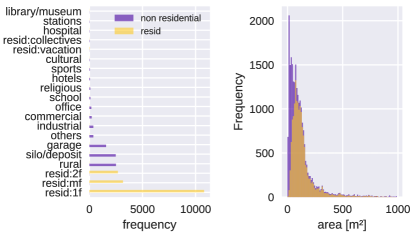
Figure 1: Statistics from RBD. Left: frequency of destination of use among the building in the AMB districts. Right: distributions of squared meter per building, conditional on being residential or not.

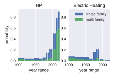
Figure 2: Probability for a building to have an HP and EH installed, conditional to the class of construction year and building destination of use.

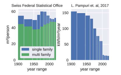
Figure 3: Representative values of m²/person (Switzerland) and kWh/m²/year (Switzerland, canton Ticino) for buildings, conditional to the class of construction year.

2.2 Component sizing

The simulated devices have been sized from the available metadata as described in the following. For the region of interest, we identified around 3000 buildings having either an installed HP or an EH, and a total installed nominal electric power of 12.5 MW and 7.7 MW for the two classes of devices. These numbers are in line with the figures that the DSO provided us with. The final distributions over the whole set of considered buildings, for some of the key metadata and device parameters, are shown in figure 4.

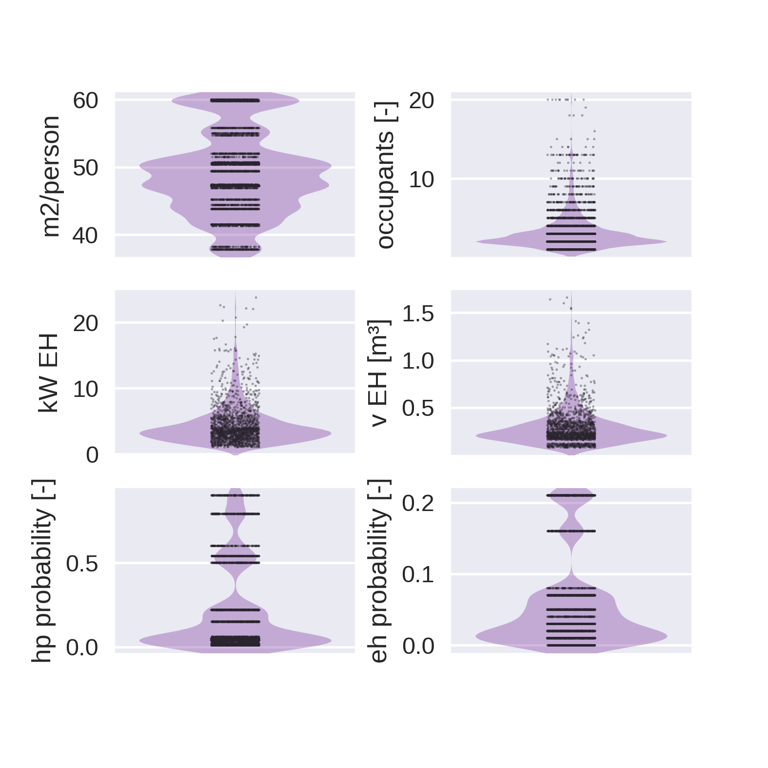
Figure 4: Final distributions of some key parameters for the simulation for the 3000 considered households

Building thermal resistance

The building’s equivalent thermal resistance could be assessed starting from the total building yearly consumption, which we previously estimated for each building from [34, 31]. Considering the following equation for a one-state RC thermal equivalent circuit:

$$\frac{\partial{T}}{dt}=R^{-1}(T_{ext}-T)+kI+Q_{int}$$ (1)

where $T_{ext}$ is the external temperature, $I$ is the global horizontal irradiance, $Q_{int}$ are internal heat gains and $k$ a coefficient. Assuming stationarity, we could retrieve an estimated thermal resistance averaging over one year:

$$R^{-1}=\frac{k\overline{I}+E_{y}}{\overline{\Delta T}}$$ (2)

where the average quantities for irradiance $I$ and temperature difference are obtained by integrating over the data of the simulated year, and $E_{y}$ is the total yearly heating consumption from [34] times the heating reference surface, expressed in kWh. The stationarity assumption, however, isn’t suitable in our context, as we have accounted for variable setpoints for the buildings’ internal temperature based on different times of the day, as it is common practice. This makes the internal temperature subject to variations during the day, which results in (2) being a poor approximation for $R^{-1}$. To better approximate it, we simulated one year of operations for each building using a simple surrogate model and optimized the value of $R$ via gradient descent, to match the annual energy consumption $E_{y}$. The detailed description of this procedure is reported in annex A.4.

Building thermal capacity

While it was possible to estimate the total equivalent resistance by cross-referencing different sources, we didn’t find any statistical source for the characterization of buildings’ equivalent thermal capacity. As for the thermal resistance, when using an RC equivalent system to simulate the thermal dynamics of the building, the C factor is usually either estimated from temporal data or in a white box fashion, starting from buildings’ stratigraphies. However, while there is a clear dependence between R and the year of construction, as shown in figure 3, due to energy-saving policies, there is no such trend for the thermal capacity. For this reason, we chose equivalent capacity factors uniformly sampling from a uniform distribution with the mean value of 2.5 MJ/m²/K and cutoff values of 1 and 5 MJ/m²/K, as these are the reference values indicated in the Swiss Society of Engineers and architects (SIA) norm 380/1 [35] for a lightweight and high inertia building.

EH sizing

The nominal power for the EH is chosen using the following formula:

$$q_{EH}=q_{DHW}=r_{v}n_{o}$$ (3)

where $r_{v}$ is a random variable drawn from the uniform distribution with limits reported in table 2, representing the $\qty{}{h}$ per person needed for heating the DHW. The variable $n_{o}=A/a(p,d)$ is the estimated number of occupants, derived from the total building area $A$, where $a(p,d)$ is the specific area per person and destination of use, $p$ and $d$ respectively, from [32] (depicted left in figure 3). The volume of the water tank is modeled similarly with the uniform distribution limits reported in 2.

HP sizing

For HP sizing, we have assumed -4 and 20 $\textdegree C$ as outdoor and indoor reference temperatures, respectively. The final nominal power for the HP is then chosen using the following formula:

$$q_{HP}=\text{maximum}\left(R^{-1}\Delta T_{ref}+q_{DHW},2\right)$$ (4)

where $R$ is the previously determined equivalent thermal resistance, $\Delta T_{ref}$ is 24 and $q_{DHW}$ is the nominal power for the domestic hot water. As previously stated, in this case, the HP is also the heating source for the DHW, which is sized as per equation (3).

2.3 Building thermal model validation

The thermal model of the building, whose parameters have been selected with the procedure explained in section 2.2, has been validated by means of annual energy consumption. The results are reported in figure 5. It can be seen how the simulated consumption is always slightly higher than the expected one (which is the annual consumption for heating from [34] multiplied by the building’s total area). This is due to the fact that the optimization procedure to tune the $R$ parameter does not include thermal losses from the heating system, and the heating system logic of the surrogate model is more reactive than the one implemented in the full simulation model, where the heating is due to serpentine. The mean relative error on the yearly energy consumption is about 5% while 90% of the simulated buildings have a discrepancy lower than 9%.

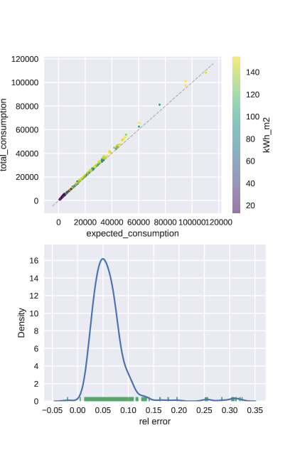
Figure 5: Validation of thermodynamic simulations by means of comparison of annual heating energy consumption for 800 randomly sampled buildings. Top: scatter plot between expected and simulated consumption. Bottom: kernel density estimation of relative error.

power [kWh/person]		volume [m3/person]
min	max	min	max
1	2	0.08	0.12

Table 2: Upper and lower bounds for the uniform distribution for the sizing of the EH

3 Energy oracle for flexibility modeling and optimization

3.1 Problem statement and methodology

We are interested in learning the aggregated power response of a group of HPs and EHs, conditional to the number of devices and a control signal, from simulations. The scope is twofold: characterizing the flexibility potential beyond simulated conditions and using the learned response to optimally craft the force-off control signal. Called $x_{t}\in\mathds{R}^{n_{f}}$ a set of $n_{f}$ features for a given simulated operational condition and a given group of devices, $y_{t}^{f}\in\mathds{R}^{H}$ their aggregated power profile for the next $H$ steps ahead, we can define a dataset of features and targets, $\mathcal{D}={(x_{t},y_{t}^{f})_{t=1}^{N}}$. The energy oracle $f(x,\theta):x_{t}\rightarrow\hat{y}_{t}^{f}$ forecasts the power consumption of a group of flexible devices starting from the features contained in $x_{t}$. Since we want to retrieve a prediction conditional to the control action, $x_{t}$ also contains information on past and future values of the control signal $s$, which is applied to the devices.

In order to learn the system response conditional to the value of the control, it is conceivable to construct a dataset consisting of paired simulations that exhibit differences solely in one control signal being zero, while all other conditions remain identical. However, it is difficult to build such a dataset, as the energy consumption of the controlled devices is affected not only by the present control signal, but also by its historical values. Eliminating this dependence would require simulating several days for each pair of rows of the final dataset $\mathcal{D}$. Instead of building a dataset of controlled and uncontrolled tuples, we just simulated a controlled year and an uncontrolled one, leaving to the oracle $f(x_{t},\theta)$ the task of modeling the causal relation between the control signal $s$ and the system response.

3.2 Dataset generation

In the context of our study, $s$ represents a binary signal that encodes the force-off state of the ripple control. This signal is restricted from random variations throughout the day and must comply with specific criteria, such as a mandated minimum period for sustained state and a capped number of daily activations. The simulated force-off signal has been obtained by generating all feasible force-off signals compatible with conditions reported in table 3. Figure 6 shows a sample of the resulting force-off signals, the ratio of scenarios in which the force-off is active as a function of time-step, and the distribution of the total steps in which the force-off signal is on. It is not possible to generate all the possible combinations of binary signals and then filter them for conditions in 3, since using a 15-minute time-step will require generating ex-ante $2^{96}$ signals. For this reason, we used a dynamic programming approach, filtering out incompatible scenarios on the run, as they are sequentially generated. We report in table 3 the criteria used to craft the evaluated scenarios.

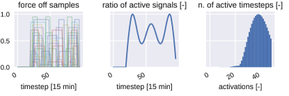
Figure 6: Left: a random sample of daily scenarios for the force-off signal. Center: ratio of active signals for a given timestep of the day. Right: distribution of the number of active timesteps among all possible scenarios.

parameter	value
force off max steps	96
min constant period	8 (2H)
max number of switches	6
max on steps	48 (12H)
nightly uncontrolled period	20 (5H)

Table 3: Parameters used to generate all possible daily force-off signals

One purpose of the oracle is to be able to predict the response of buildings in different portions of the distribution grid. Instead of training several oracles based on the number of buildings equipped with an HP or an EH, we follow suggestions from forecasting literature, where global models are effectively trained to predict time series coming from different sources. Following this approach, we introduce penetration scenarios in the training dataset, using the following procedure:

1. Run two full-year simulations for the whole set of modeled buildings; the first year is subject to the daily force-off scenarios sampled at random out of the possible ones, while the second year is simulated without controlling the devices.

2. Build penetration scenarios, grouping a subset of the simulated buildings, from which the aggregated power, $y_{t}^{f}$ is retrieved. For each penetration scenario, a dataset is then built picking at random $k\%$ observations from the simulated years. We sampled a total of 100 penetration scenarios and used $k=20$, for a total length of the dataset of 40 equivalent years.

3. Retrieve metadata describing the pool of buildings for each penetration scenario. Metadata includes the total number of each kind of device, the mean thermal equivalent transmittance (U) of the sampled buildings, and other parameters reported in table 4. We further augment the dataset with time features such as the hour, the day of the week, and the minute of the day of the prediction time.

4. Augment each penetration scenario dataset through transformations and lags of the original features, as reported in table 5, to obtain $\mathcal{D}_{s}$.

5. Retrieve the final dataset by stacking the penetration scenario datasets $\mathcal{D}=[\mathcal{D}_{s}]_{1:n_{s}}$

penetration scenario features	temporal features
p_nom_tot, p_q_10, p_q_90, n_hp, n_eh, device_ratio, U_mean, U_q_10, U_q_90, C_mean, C_q_10, C_q_90	hour, day of week, minuteofday

Table 4: Metadata used as features in the training set. Penetration scenario features describe the characteristics of the pool of simulated buildings and devices, while temporal features refer to the time of the prediction.

signals	transformation	lags
force off	mean(15m) mean(3h), mean(6h)	-95,…96 1…96
$y_{t}^{f}$, meteo	mean(15m) mean(1h)	-4,..0 -168..-144, -24…0
meteo	mean(1h)	1..24

Table 5: Continuous variables, transformations and lags passed as features to the oracle. Meteorological information consists of temperature and global horizontal irradiance measurements.

3.3 Model description

The energy oracle is a collection of multiple-input single-output (MISO) models, each of which is a LightGBM regressor [36] predicting $y_{t}^{f}$ at a different step-ahead. The alternative to a collection of MISO models is training just one MISO model after augmentation of the dataset with a categorical variable indicating the step ahead being predicted. This option was discarded due to both memory and computational time restrictions. For our dataset, this strategy requires more than 30 GB of RAM. Furthermore, the training of a single tree for the whole dataset requires more computational time than training a set of MISO predictors in parallel (on a dataset that is 96 times smaller).

We recall that the final dataset is composed of 100 scenarios differing in the set of buildings composing the aggregated response to be predicted. This means that removing observations at random when performing a train-test split would allow the oracle to see the same meteorological conditions present in the training set. To overcome this, the training set was formed by removing the last 20% of the yearly observations from each penetration scenario dataset $\mathcal{D}_{s}$. That is, the training-test split is done such that the training set contains only observations relative to the first 292 days of the yearly simulation.

A hyperparameter optimization is then run on a 3-fold cross-validation over the training set; this means that each fold of the hyperparameter optimization contains roughly 53% of $\mathcal{D}$. The tuned hyperparameters are just the learning rate and the number of estimators for the LightGBM regressors; the parameters are kept fixed for all 96 models predicting the various step-ahead. We used a fixed-budget strategy with 40 samples, using the optuna python package [37] implementation of the tree-structured Parzen estimator [38] as a sequential sampler. An example of loss landscape for the hyperparameter optimization is shown in figure 7.

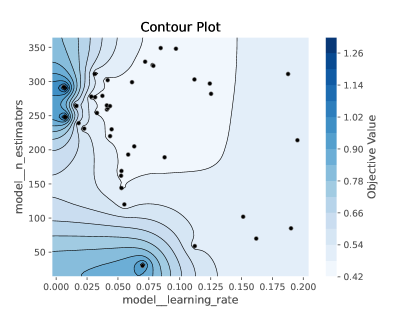
Figure 7: Loss landscape for the hyperparameter tuning in 3 folds cross-validation for the base energy oracle with random sampling strategy.

3.4 Ablation studies

We performed an ablation study on the model in order to see the effectiveness of different sampling strategies for the dataset formation and model variations.

Sampling schemes

We tested two different sampling schemes for producing the penetration scenarios to generate the final dataset. In the first strategy, the total number of controllable devices is increased linearly, picking randomly between households with an HP or an EH. In the second strategy, the number of controllable devices is increased independently co-varying the number of HPs and EHs, in a cartesian fashion.

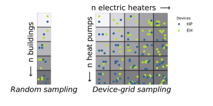
Figure 8: Sampling strategies for building the final training set. Left: the total number of controllable devices is increased linearly, picking randomly between households with an HP or an EH. Left: the number of controllable devices is increased by independently co-varying the number of HPs and EHs.

Energy unbalance awareness

One physical insight that could help increase the accuracy of the power oracle, is the energy unbalance. The idea is the following: we can use the oracle to predict twice the response of the system: once with the actual control signal $s$ and once with the control signals equal to $s_{ref}$ (which correspond to a zeroed force-off signal in the case of ripple control). We can then subtract the two responses to get an ”energy debt” of the system for each timestep. It is reasonable to think that, under well-calibrated controllers, the energy debt will balance out on a long enough prediction horizon. Even if this is not the case, having the information about the energy debt in which the system occurred at each time step could help predict the successive ones. For this reason, we tested a second model, in which, at first, a set of regressors predict the system response for all the steps ahead with and without the future force-off signals zeroed out. The two predictions are then subtracted to obtain the energy unbalance, and this information is used to augment the training set. Finally, another set of regressors is trained on this new dataset. The same strategy is deployed at prediction time.

In total, we compared four distinctive configurations, comprising two models and two sampling strategies. Specifically, the models reviewed included:

• A set of 96 independent LightGBM models, predicting the 96 steps ahead independently.

• An energy-aware set of 96 LightGBM models, linked by the energy unbalance previously described.

Simultaneously, we employed two different sampling methodologies:

• Random sampling of the number of HP and EH.

• Grid sampling, executed at equidistant intervals for the number of HP and EH.

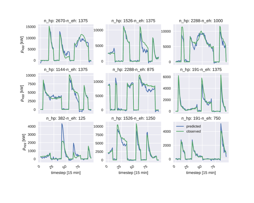
Figure 18: Random example of day-ahead power oracle predictions, for different numbers of HPs and EHs, where the force off was activated at least once.

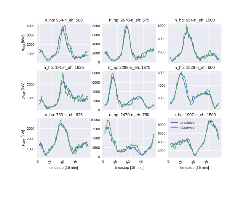
Figure 19: Random example of day-ahead power oracle predictions, for different numbers of HPs and EHs, where the force off was not active.

To gain an intuitive understanding of the oracle’s performance, we direct the reader to Appendix B. Within this section, Figures 18 and 19 provide representative examples from the test set, featuring varying counts of controlled heat pumps (HPs) and electric heaters. These illustrations stem from the energy-aware oracle trained utilizing the grid sampling strategy and represent both uncontrolled and controlled scenarios, respectively.

To study the error dependencies on various influencing factors, we generated a heatmap illustrating the Normalized Mean Absolute Error (NMAE) as a function of the overall nominal power of the predicted samples and the step-ahead, depicted in Figure 9. There appears to be a notable correlation between oracle accuracy and aggregated loads, an anticipated outcome considering the regularization effect of aggregation, which enhances the predictability of $p_{agg}$. The NMAE descends to values as low as 0.12 for the first step-ahead, increasing to 0.28 when the nominal power ranges between 2 and 5 MW. No significant differences are detected across the four models under investigation. To further investigate the accuracy with respect to prediction timing, a similar aggregation was executed, displayed in Figure 10. The models demonstrate superior predictive capability during nighttime hours, whereas the NMAE surges during peak periods. Analogous to the prior analysis, no noteworthy differences emerge among the various models

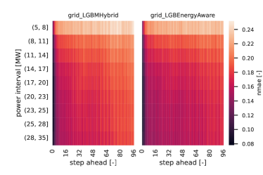
Figure 9: NMAE for the two tested models for the power oracle, when using grid samples, as a function of step-ahead and total nominal power of predicted samples.

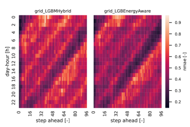
Figure 10: NMAE for the two tested models for the power oracle, when using grid samples, as a function of step-ahead and time of prediction.

Models performances can be better compared when plotting the mean NMAE as a function of step ahead, as done in figure 11. The grid sampling scheme did indeed help in increasing the accuracy of the predictions w.r.t. the random sampling scheme for both the LightGBM models. Including the information about energy unbalances at each step ahead shows some benefits for both sampling strategies, at the expense of a more complex overall model. The accuracy improvement impacts only on controlled scenarios, as demonstrated by a comparison of the second and third panels in figure 11. These panels show the scores obtained for instances where the force-off signal was activated at least once or never activated. This result aligns with our expectations. As an additional analysis, we studied the energy unbalance over the prediction horizon. For this analysis, we considered just the controlled cases in the test set. We define two relative energy unbalanced measures:

$$\Delta_{rel}E_{d}=\frac{\sum_{t=1}^{96}\hat{y}_{t}(s)-\sum_{t=1}^{96}y_{t}}{\sum_{t=1}^{96}y_{t}}$$ (5)

$$\Delta_{rel}^{noctrl}E_{d}=\frac{\sum_{t=1}^{96}\hat{y}_{t}(s)-\sum_{t=1}^{96}\hat{y}_{t}(s_{0})}{\sum_{t=1}^{96}y_{t}}$$ (6)

where $y_{t}$ is the simulated power, $\hat{y}(s)$ is the power predicted by the oracle with the control used in the simulation, and $\hat{y}(s_{0})$ is the power predicted by the oracle using a zero force off. We can interpret $\Delta_{rel}E_{d}$ and $\Delta_{rel}^{noctrl}E_{d}$ as the relative error in the total energy need w.r.t. the simulation and the change in the energy consumption estimated by the oracle if the pool of flexible devices were not controlled. We removed from the comparison all the instances in which the force-off signal was activated in the last 5 hours of the day. In this case, part of the consumption will be deferred outside the prediction horizon, making the comparison meaningless.

Looking at the first row of figure 12, we see how the empirical cumulative distribution functions (ECDFs) of $\Delta_{rel}E_{d}$ and its absolute value (left and right panels) are closer to zero when the model considers information on the energy unbalance. Also applying the grid sampling strategy helps in having a more precise prediction in terms of used energy over the prediction horizon. For all 4 models, 80 % of the time the relative deviation in the horizon energy prediction lies below 20%. The second row of figure 12 reports the change in the forecast energy consumed within the prediction horizon with and without control. It is reasonable to think, also in this case, the consumption should approximately match, since the force off usually just defers the consumption. Also in this case, the energy-aware models present a lower difference in the consumed energy.

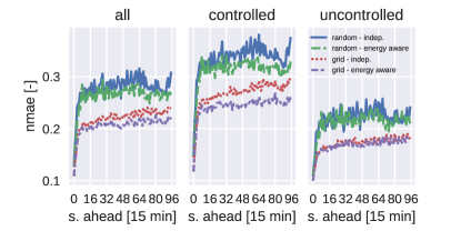
Figure 11: Performances for the four tested models for the power oracle, in terms of NMAE as a function of the step ahead.

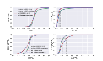
Figure 12: Left: cumulative un-normalized distribution of the relative energy unbalance error. Right: inverse cumulative function of the absolute normalized energy unbalance.

3.5 Characterization of the rebound effect

We finally used the energy unbalance aware model in combination with the grid sampling strategy to visualize rebound effects for different numbers of HPs and EHs. Figure 13 shows three extreme examples of the characterization: the penetration scenario with the maximum number of EHs and zero HPs, the converse, and the scenario where both penetrations are at their maximum value. The rebound is shown in terms of energy unbalance from the test set, such that they have a force-off signal turning off at the fifteenth plotted step. It can be noticed how different observations can start to show negative energy unbalance at different time steps; this is due to the fact that force-off signals can have different lengths, as shown in figure 6. The upper left quadrant shows the energy unbalance predicted by the oracle in the case of the maximum number of EHs and no HPs. Comparing it with the lower right quadrant, where the sample just contains HPs, we see a much smaller tau; that is, the rebound effect has a quicker decay, being close to zero after only 10 steps (corresponding to 1 and a half hours). The lower right quadrant exhibits a markedly slower dissipation of the rebound effect, attributable to the different heating mechanisms and temporal constants inherent in systems heated by EHs and HPs. EHs, dedicated solely to DHW heating, have their activation guided by a hysteresis function governed by two temperature sensors installed at varying heights within the water tank. In contrast, HPs are responsible for both DHW and space heating, and their activation hinges on the temperature of the hydronic circuit, thus creating a segregation between the HPs and the building heating elements, namely the serpentine. As a result, HPs’ activation is subject to a system possessing a heating capacity significantly greater than that of the standalone DHW tank: the building’s heating system. Further intricacy is added to the power response profile of the heat pump due to its dual role in catering to DHW and space heating needs, with priority assigned to the former. The visual responses presented in Figure 6 are color-differentiated according to the seven-day mean of the ambient temperature. As per the expected pattern, the EHs’ responses exhibit independence from the average external temperature, while a modest influence can be detected for the HPs, where a rise in average temperatures aligns with a faster decay in response.

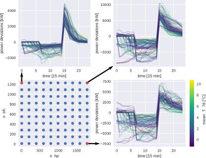
Figure 13: Example of system response in terms of deviations from the expected response (prediction where control signal features referring to feature time-steps are zeroed), dependent on the number of HPs and EHs.

4 Energy oracle for optimal flexibility control

In this section, we present how the energy oracle can be incorporated into the optimization loop, beginning with optimizing a single flexibility group. The objective that we found most compelling from both the DSO and energy supplier perspectives is the simultaneous minimization of day-ahead costs (incurred by the energy supplier on the spot market) and peak tariff (borne by the DSO to the TSO). Notably, this scenario is particularly well-suited to Switzerland, where a distinctive situation persists with the energy supplier and the DSO remaining bundled. The peak tariff, being proportionate to the maximum monthly peak over a 15-minute interval, poses a more significant optimization challenge in comparison to day-ahead costs, as it requires resolving an optimization issue over a full month. Due to this extensive duration, the possibility of achieving accurate power forecasts is extremely hard. As a heuristic solution, we manage this issue on a daily basis. Operating under the presumption that if the DSO systematically diminishes its peak each day of the month, a reduction in the monthly peak will follow. This then leads us to the following optimization problem:

$$s^{*} =\underset{s}{\text{argmin}}\,\gamma\mathcal{L}(\hat{y}(s))$$ (7)

$$=\underset{s}{\text{argmin}}\,\left(\sum_{h=1}^{H}p^{s}_{h}\hat{y}_{h}(s)\right)+p^{p}\max(0,\max_{h}\hat{y}_{h}(s)-y^{max}_{k})$$ (8)

where $h$ refers to the step ahead, $p^{s}\in\mathds{R}^{T}$ is the day-ahead spot price, $p^{p}$ is the price for the monthly peak in $CHF/kW$, $\gamma=dt/3600$ is a coefficient taking into account the timestep. The second term in equation (8) encodes the cost of increasing the peak realized so far in the current month, $y^{max}_{k}$. Problem (7) is not trivial to solve since it’s a function of a non-parametric regressor, the energy oracle. However, the parameters reported in table 3 produce a total of 155527 control scenarios; this allows us to evaluate (7) using a brute-force approach, finding the exact minimizer $s^{*}$. This is done through the following steps:

1. Forecast the total power of the DSO: $\hat{y}^{tot}=f_{tot}(x_{t},\theta_{tot})$. This forecaster was obtained by training 96 different LightGBM models, one for each step ahead.

2. Forecast the baseline consumption of flexible devices, $\hat{y}^{f}(s_{0})=f(x_{t},s_{0},\theta)$, using the energy oracle with the control signal $s=s_{0}$ set to zero (corresponding to not controlling the devices).

3. Forecast the response of flexible devices under a given control scenario $s$ for the next day. This is always done using the energy oracle: $\hat{y}^{f}(s)=f(x_{t},s,\theta)$.

4. The objective function is evaluated on $\hat{y}_{t}(s)=\hat{y}^{tot}-\hat{y}^{f}(s_{0})+\hat{y}^{f}(s)$ for all the possible plausible control scenarios; the optimal control scenario $s^{*}$ minimizing the total costs is returned.

4.1 Controlling multiple groups

As previously noted, forcing off a group of flexibilities results in a subsequent rebound effect when they are permitted to reactivate. A viable strategy to counter this issue is to segment the flexibilities into various groups, thereby circumventing a concurrent reactivation. Moreover, this segmentation method helps exploit their thermal inertia to the fullest extent. This is especially true in the context of heat pumps, as variations in building insulation and heating system sizing inevitably lead to differences in turn-on requirements to maintain home thermal comfort under identical weather conditions. Analogous considerations apply to hot water boilers as well. In addition, it is crucial to note that generally, EHs can endure longer force-off periods compared to HPs. Thus, the stratification of flexibilities into distinct groups not only mitigates the rebound effect but also facilitates the optimal utilization of the entire appliance fleet’s potential. Problem (7) can be reformulated as:

$$s^{*}=\underset{[s_{g}]_{g=1}^{G}}{\text{argmin}}\, \sum_{h=1}^{H}p^{s}_{h}\left(\hat{y}_{h}^{tot}-\sum_{g=1}^{G}\hat{y}_{h,g}^{f}(s_{0})+\sum_{g=1}^{G}\hat{y}_{h,g}^{f}(s_{g})\right)+$$ (9)

$$p^{p}\max_{h}\sum_{h=1}^{H}\left(\hat{y}_{t}^{tot}-\sum_{g=1}^{G}\hat{y}_{h,g}^{f}(s_{0})+\sum_{g=1}^{G}\hat{y}_{h,g}^{f}(s_{g})\right)$$ (10)

where $G$ is the total number of groups and $s_{g}$ is the control signal sent to the $g_{th}$ group. Problem (9) is a combinatorial problem; to reduce its complexity, we have used a sequential heuristic: the first group of devices optimizes on the uncontrolled power profile $\hat{y}_{t}^{tot}$. Once their optimal control for the first group is found, the second group it’s optimally scheduled on $y_{t}^{tot}-\hat{y}_{t,1}^{f}(s_{0})+\hat{y}_{t,1}^{f}(s)$, where the second subscript in $\hat{y}_{t,1}$ refers to the control group. An example of such sequential optimization is shown in figure 14 where one group of EHs and one of HPs are scheduled sequentially.

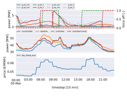
Figure 14: Example of optimized control action using the energy oracle. Top: control signals (dashed), forecast group responses (dotted) and simulated, both controlled and uncontrolled, response (thick). Middle: total power from uncontrolled DSO’s households (blue), total DSO’s power when no control action is taken (orange), simulated and forecasted system response (green and red). Bottom: day-ahead price on the spot market.

The upper panel shows the optimal control signals, along with the simulated response (dashed lines) and the response predicted by the energy oracle (dotted lines). The middle panel shows the power from uncontrolled nodes in the DSO’s grid (blue), the total DSO’s power when no control action is taken (orange), simulated and forecast system response (green and red).

4.2 Ensuring comfort for the end users

To ensure end-user comfort while leveraging their flexibility, it is critical to ensure that appliances maintain the ability to meet energy demands for a certain period of time, despite shorter time shifts within this duration. When a building is heated with a thermo-electric device such as a heat pump (HP), its energy consumption exhibits a significant inverse correlation with the external temperature. This correlation can be effectively illustrated using an equivalent linear RC circuit to model the building’s thermal dynamics. The static behavior of this model can be represented by the energy signature, which depicts the linear relationship between the building’s daily energy consumption and the mean daily external temperature, denoted as $T_{d}$. As more households now feature photovoltaic (PV) power plants, it becomes relevant to include the average daily global horizontal irradiance, or $I_{d}$, as a contributing factor in the energy signature fit. As a first approximation, we assume a linear relationship between global irradiance and PV production. Consequently, elevated $I_{d}$ values may correspond to lower daily energy consumption, granted a PV system is installed. However, such an effect should not be misattributed to variations in temperature. Failing to integrate $I_{d}$ into the regression could lead to an underestimation of the daily energy consumption when expressed as a function of temperature. The comprehensive energy signature, denoted as $e(T_{d},I_{d})$, emerges as a piecewise linear function reliant on the external temperature and $I_{d}$. Figure 15 provides an exemplification of an estimated energy signature.

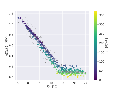
Figure 15: Energy signature example. The average daily consumption for a household is estimated with a (piece-wise) linear function of temperature and solar irradiance. Gray dots: original observations. Crosses: fit results, colored by $I_{d}$

Our ultimate objective is to ascertain the necessary operational duration for a specified HP to fulfill the building’s daily energy requirements. Consequently, the total number of active hours during a day, $h$, is obtained by dividing the energy signature by the nominal power of the HP:

$$h(T_{d},I_{d})=\frac{e(T_{d},I_{d})}{p_{nom}}$$ (11)

The following steps describe our procedure to generate and control a group of HPs based on their estimated activation time:

1. Estimate the energy signatures of all the buildings with an installed HP $e_{i}(T_{d},I_{d})$

2. Estimate their reference activation time $h_{ref,i}$ for worst-case conditions, that is, for $T_{d}=0$ and $I_{d}=0$.

3. At control time, perform a day-ahead estimation of activation times for all the HPs, $h_{i}(\hat{T}_{d},\hat{I}_{d})$ using a day-ahead forecast of $T_{d}$ and $I_{d}$. Use the within-group maximum values of the needed activation time, $h_{max,g}=\max_{i\in\mathcal{G}}h_{g,i}(\hat{T}_{d},\hat{I}_{d})$ to filter out control scenarios having more than $h_{max,g}$ force-off steps. This process guarantees that all HPs are allowed on for a sufficient time, given the temperature and irradiance conditions.

5 Energy oracle for closed loop emulations

For testing operational and closed-loop accuracy, we simulated one year of optimized operations, in the case in which 66% of the available flexibilities are controlled. We used two control groups: one containing only EHs, which can be forced off for a longer period of time, and one group of HPs, controlled as explained in the previous section.

The prediction error accuracy was already studied in section 3.4, where we tested the oracle on a simulated test set. In that case, the force-off included in the dataset were random, as we couldn’t already optimize them. We further tested the performance of the energy oracle when predicting the optimized force-off. The difference is that the actual optimal force-off is more correlated than the random ones observed during training, and the performance could be different. Besides this, we also assessed the accuracy of the oracle in terms of economic results in closed-loop; that is, we retrieve the errors on the economic KPIs when the simulation is completely bypassed and the oracle is used for both optimizing and emulating the behaviour of the controlled devices.

5.1 Open loop operational accuracy

At first, operational accuracy was assessed in terms of predictions, comparing the aggregated controlled power profile with the sum of the individually simulated (controlled) devices. Figure 16 shows the normalized daily time series of the prediction error during the actual optimization process. This is defined as:

$$n\epsilon_{d}=\frac{y_{d}-\hat{y}_{d}}{y_{d}}$$ (12)

where $y_{d},\hat{y}_{d}\in\mathds{R}^{96}$ are the aggregated simulated power profiles and their day ahead predictions, respectively. We see that for all the observed error paths we just have sporadic deviations above 10%. To have a more general understanding of the oracle performance, in the second panel of 16 we plotted the histogram of the mean daily error, defined as $\frac{1}{96}\sum_{i=1}^{96}nE_{d,i}$. This shows that the energy oracle is usually under-predicting, or over-smoothing, the true response from the simulation, which is, in general, the expected behavior of a forecaster trained to minimize the sum of squares loss. The fact that this distribution is contained in the -2%+2% interval, which is much narrower than in the maximum observed discrepancies in the daily error traces, confirms that high error deviations in the day ahead predictions are just sporadic.

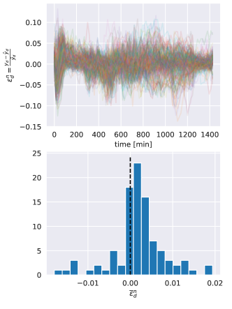
Figure 16: Performance of the oracle in the open-loop simulations. Left: daily relative errors plotted as time series. Right: distribution of the daily means of the relative error.

5.2 Closed loop economic performances

We cannot directly assess the closed-loop performances of the oracle in terms of prediction errors. This is due to the fact that, when simulating in a closed loop, the predictions of the oracle are then fed to itself in a recurrent fashion. This could result in slightly different starting conditions for each day; furthermore, the comparison of the sampled paths is not our final goal. A more significant comparison is in terms of economic returns. We compared these approaches:

1. Simulated: we run the optimization and fully simulate the system’s response. In this setting, the oracle is just used to obtain the optimal control signal to be applied the day ahead. The controlled devices are then simulated, subject to the optimal control signal. The costs are then computed based on the simulations.

2. Forecast: for each day, the optimal predictions used for the optimization are used to estimate the cost. We anyways simulate the controlled devices; this process is repeated the next day. This approach gives us an understanding of how the operational prediction errors shown in figure 16 impact the estimation of the costs.

3. Emulated: the simulations are completely bypassed. The oracle is used for both optimizing the control signal and generating the next-day responses for the controlled devices.

It should be clear that, if the third approach gives comparable results in terms of costs, we could then just use the energy oracle for both the control task and its evaluation. This would significantly speed up the simulation loop: we won’t have to simulate the thermodynamic behavior of thousands of households, but just evaluate the trained oracle, which evaluation is almost instantaneous. It could seem unlikely to reach the same accuracy produced by a detailed simulation, but this can be justified by the fact that we’re only interested in an aggregated power profile, whose dimensionality is just a tiny fraction of all the simulated signals needed to produce it.

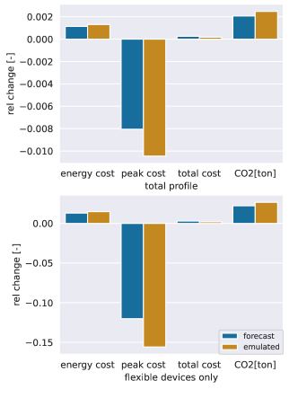
Figure 17: Deviations of different objectives from the simulated results, using the energy oracle to optimize and forecast the power profiles (blue) or to completely bypass the simulation (orange). Top: relative error of objectives normalized with the total simulated costs. Bottom: relative error of objectives normalized with the additional costs faced by the DSO due to the flexible group.

In figure 17, we reported the relative discrepancies from economic KPIs retrieved by the simulation, using the two aforementioned approaches. As an additional KPI, we also reported the estimated tons of produced $CO_{2}$. While the $CO_{2}$ emissions are not directly optimized for, minimizing the energy costs also have a positive impact on the emissions, since energy prices correlate with the $CO_{2}$ intensity in the energy mix. The emitted $CO_{2}$ tons are estimated as:

$$M_{C0_{2}}=\sum_{t=1}^{T}C_{t}y_{t}$$ (13)

where $C_{t}$ is the carbon intensity in the national energy mix in $\frac{g_{CO_{2}}}{kWh}$. The top panel refers to the costs that would generate considering the total power profile, $y$. All the costs, in both the forecast and closed-loop cases, have a deviation of less than 1%. The total cost has a deviation of well below 1 per thousand. In our case study the controlled group of devices is just a small fraction of the total energy delivered by the DSO; to estimate the oracle’s performance it’s thus important to evaluate only costs generated by controlled devices $y^{f}$. These are shown in the bottom panel of figure 17, where we have normalized the objectives’ errors with the additional costs faced by the DSO due to the flexible group: both the energy costs and the $CO_{2}$ we have a relative error below the 3% , while the peak cost has a deviation of 6%. We have a comparable deviation for forecasts and closed-loop simulations. In all the cases, the peak costs are underestimated; this was to be expected, as the oracle is trained with a sum of squares loss, which systematically underestimates extreme events.These discrepancies can still be considered reasonable to perform A/B testing in simulation.

	simulated	$\Delta_{rel}$ forecasts	$\Delta_{rel}$ closed loop
Energy	4.18E+7	1.13E-3	1.30E-3
Peak	4.46E+6	-8.05E-3	-1.05E-2
Total	4.62E+7	2.47E-4	1.68E-4
$CO_{2}$[ton]	5.99E+4	2.06E-3	2.48E-3

Table 6: First column: costs of energy, peak, total costs, and $CO_{2}$ emissions from the controlled simulation. Second column: relative differences from the simulated costs when they are evaluated using the day-ahead predictions from the oracle. Third column: relative differences from the simulated costs using the oracle to emulate the system. Data refers to the case in which 66% of the available HPs and boilers were controlled.

	simulated	$\Delta_{rel}$ forecasts	$\Delta_{rel}$ closed loop
Energy	3.65E+6	1.29E-2	1.49E-2
Peak	2.99E+5	-1.2E-1	-1.56E-1
Total	3.95E+6	2.88E-3	1.97E-3
$CO_{2}$[ton]	5.58E+3	2.21E-2	2.65E-2

Table 7: First column: additional costs of energy, peak, total costs, and $CO_{2}$ emissions faced by the DSO due to the flexibility group. Second and third columns as for table 6

The left panel shows discrepancies for actual costs faced by the DSO, computed using the total power profile $y$. In this case, we have roughly a ten-fold reduction in the relative error w.r.t. the simulations. This is not a surprise, since as anticipated, the controllable devices constitute only a fraction in terms of energy supplied by the DSO. Nevertheless, this is the quantity we are interested in. For completeness, the relative deviations and absolute costs for the simulated case relative to figure 17 are reported in tables 6 and 7 for the total and flexible device profiles, respectively.

6 Conclusions and extensions

In this work, we presented a methodology to model the flexibility potential of controllable devices located in a DSO’s distribution grid and optimally steer it by broadcasting force-off signals to different clusters of flexible devices. We achieved this by training a non-parametric global forecasting model conditional to the control signals and the number of controlled devices to predict their simulated aggregated power. The numerical use case showed that the forecaster’s accuracy is high enough to use it as a guide to optimally steer deferrable devices. Moreover, the high accuracy on economic KPIs suggests that the forecaster can be used to completely bypass the simulation and speed up A/B-like testing and the retrieval of different demand-side management policies over different penetration of devices.
We envision the following possible extensions of the presented work:

• Continuous control. The presented use case relied on extensive enumeration of the possible force-off signals for the day ahead optimization. This was possible due to restrictions requested by the DSO on the shape of the control signal, which resulted in a total number of possible control signals in the order of 1e5 scenarios. Using a higher timestep for the control will require evaluating a prohibitive number of scenarios. The approach proposed in this paper can still be feasible by replacing the boosted tree with an ”optimizable” regressor, that is, either a partial input-convex neural network [39] or a conditional invertible neural network [40]. In this case, we can use a continuous signal $s_{c}\in[0,1]$ indicating the fraction of flexible devices to be forced off at a given moment in time. We can then apply gradient descent to the optimizable regressor and retrieve the optimal $s_{c}$.

• Probabilistic forecast. The presented optimization framework is based on a deterministic formulation. Formulating the problem in the stochastic framework could be advantageous when considering peak tariffs. This would require summing two sources of uncertainty: the one associated with the prediction of the total power profile $y^{tot}$ and the one associated with the energy oracle forecasts. These can be both assessed by obtaining probability distributions after the training phase through conformal prediction and using them to generate scenarios.

Appendix A Thermal models

A.1 Control logic of heating systems

The heat pump control logic is based on two temperature sensors placed at different heights of the water tank, while the circulation pump connecting the tank with the building’s heating element is controlled by a hysteresis on the temperature measured by a sensor placed inside the house.
We describe the control logic in a sequential way, following the heating components of the system. The first decision is taken by the building central controller, which decides its working mode, that is, if the building needs to be cooled or heated, based on a moving average of the historical data of the external temperature:

$$\begin{cases}wm_{t}&=-1\qquad\textbf{if}\quad T_{ma,t}>T_{max,ma}\\ wm_{t}&=\ \ 1\qquad\textbf{if}\quad T_{ma,t}<T_{min,ma}\\ wm_{t}&=\ \ 0\qquad otherwise\end{cases}$$ (14)

where the working mode $wm_{t}$ is negative when the building requires to be cooled, positive when heating is required, and 0 when no actions are needed.$T_{max,ma}$ and $T_{min,ma}$ represent the maximum and minimum values of the external temperature’s moving average, which is based on the past 7 days. The actual activation of the heating element is controlled by the hysteresis on the internal temperature of the building, $T_{z}$. If the working mode is positive, this is given by:

$$\begin{cases}s_{hy,t}&=1\qquad\textbf{if}\quad\left(\ T_{z}<T_{min,hy}-\Delta T/2\right)\\ &\qquad\quad\ \textbf{or}\quad\left(T_{z}<T_{min,hy}+\Delta T/2\quad\textbf{and}\quad s_{hy,t-1}\right)\\ s_{hy}&=0\qquad otherwise\\ \end{cases}$$ (15)

where $s_{hy,t}$ is the state of the hysteresis at time $t$, 1 meaning that the circulation pump of the heating element must be activated, and $\Delta T$ was chosen to be equal to 1${}^{\circ}C$. For completeness, we report also the control logic when the building is in cooling mode:

$$\begin{cases}s_{hy,t}&=1\qquad\textbf{if}\quad\left(\ T_{z}>T_{max,hy}+\Delta T/2\right)\\ &\qquad\quad\ \textbf{or}\quad\left(T_{z}>T_{max,hy}-\Delta T/2\quad\textbf{and}\quad s_{hy,t-1}\right)\\ s_{hy}&=0\qquad otherwise\\ \end{cases}$$ (16)

The incoming water temperature in the heating element is then modulated linearly through a 3-way valve between a maximum and minimum value, based on the external temperature, both in the heating and cooling modes. When operative, the heating element requests hot or cold water to the water tank, which control logic is based on two temperature sensors located in two different layers. When the building is in heating mode, the control logic is a simple hysteresis based on the temperature of the sensor in the uppermost layer, which is identical to the one in (15). When in cooling mode, the control logic is the following:

$$\begin{cases}s_{hy,t}&=-1\qquad\textbf{if}\quad\left(\ T_{up}>T_{max}^{c}+\Delta T/2\right)\\ &\qquad\qquad\ \textbf{or}\quad T_{low}>T_{max}^{c}+\Delta T/2\\ s_{hy,t}&=0\qquad\quad\textbf{if}\quad\left(\ T_{low}<T_{min}^{c}\right)\ \textbf{or}\left(T_{up}<T_{max}^{c}-\Delta T/2\right)\\ s_{hy,t}&=s_{hy,t-1}\quad otherwise\end{cases}$$ (17)

where $T_{up}$ and $T_{low}$ are the temperature measured by the upper and lower sensors, respectively, and $T_{min}^{c}$ and $T_{max}^{c}$ are the minimum and maximum desired temperatures of the water in the tank while in cooling mode.
The value of $s_{hy,t}$ is then communicated to the HP. In the case in which the HP is also used for the domestic hot water (DHW), the DHW tank is always served with priority by the HP.

A.2 Heat distribution system

Floor heating was modeled starting from the first principles. Considering a fixed and uniform temperature for the ground and the building internal temperature at each time-step and stationary conditions, we can retrieve the analytical expression of the temperature profile along the pipe, through the energy balance on an infinitesimal element of the pipe. This can be expressed as:

$$\frac{\partial cT_{x}}{\partial t}=\Phi_{x}-\Phi_{x+\partial x}+\dot{q}_{up}+\dot{q}_{down}$$ (18)

where $c$ is the heat capacity in $J/K$, $x$ is the distance from the pipe entrance, $T_{x}$ is the temperature of the water inside the pipe at $x$, $\Phi$ are enthalpy flows at the entrance and exit of the considered infinitesimal volume, $\dot{q}_{up}$ and $\dot{q}_{down}$ are the heating powers from the building and from the ground. Expressing the latter through equivalent resistance taking into account convective and conductive effects, the balance in steady state can be rewritten as:

$$\frac{\dot{m}c_{p}}{\rho^{*}}\frac{\partial T_{x}}{\partial x}=\frac{R_{down}T_{z}+R_{up}T_{g}}{R_{down}+R_{up}}-T_{x}=T^{a}-T_{x}$$ (19)

where $T^{a}$ is the asymptotic temperature and where:

$$R_{down} =\frac{1}{h_{in}w}+\frac{1}{h_{u,eq}w}+R_{u}$$ (20)

$$R_{up} =\frac{1}{h_{in}w}+R_{g}$$ (21)

$$\rho^{*} =\frac{R_{up}+R_{down}}{R_{up}R_{down}}$$ (22)

where $w$ is the diameter of the tube, $h_{in}$ is the internal coefficient of heat transfer, which can be retrieved using available empirical relation for fully developed flow with fixed temperature at the boundary conditions [41], $h_{u,eq}$ is the heat transfer coefficient between the floor and the building air including both the effect for natural convection and radiation. The values of $h_{u,eq}$ can be found in the literature [42]. The value of the thermal resistances $R_{u}$ and $R_{g}$, towards the floor and the ground, can be found in the literature as well. We can reformulate (19), making it adimensional through a change of variable:

$$\frac{\partial\Theta}{\partial\mathcal{X}}=-\Theta$$ (23)

from which solution we can retrieve the temperature profile of the water inside the pipe:

$$T_{x}=T^{a}+(T_{0}-T^{a})e^{\frac{-x\rho^{*}}{\dot{m}c_{p}}}$$ (24)

where $T_{0}$ is the temperature of the water at the pipe inlet. We can use (24) to retrieve the heating power flowing into the building, integrating $\dot{q}_{up}(x)$ along the pipe.

$$\dot{Q}_{up}=\int_{0}^{L}\dot{q}_{up}(x)\mathrm{d}x=\int_{0}^{L}\frac{T(x)-T_{z}}{R_{up}}\mathrm{d}x$$ (25)

where $L$ is the length of the serpentine. Integrating, we obtain

$$\dot{Q}_{up}=\frac{(T^{a}-T_{z})L-(T_{L}-T_{0})\frac{\dot{m}c_{p}}{\rho^{*}}}{R_{up}}$$ (26)

where $T_{L}$ is the temperature of the water at the outlet of the serpentine. Note that the equation (26) tends to $(T_{L}-T_{0})\dot{m}c_{p}$ when $R_{down}$ increase and $R_{up}$ is kept fixed.
The nominal mass flow of the heating system and the length of the serpentine are found as the solution of the following optimization problem:

$$\underset{L,\dot{m}}{\text{argmin}}\,\left(\dot{Q}_{up}(L)-\dot{Q}_{nom}\right)^{2}+10^{-3}\left(\dot{m}-\dot{m}_{nom}\right)^{2}$$ (27)

where $\dot{m}_{nom}$ is a reference mass flow, equal to $0.1\left[kg/s\right]$ and $\dot{Q}_{nom}$ is the power required to keep the building internal temperature constant under reference conditions (we used an external temperature of -4${}^{\circ}C$ and a desired internal temperature of 20 ${}^{\circ}C$):

$$\dot{Q}_{nom}=\frac{\Delta T_{ref}}{R}$$ (28)

where $R$ is the resistance of an equivalent RC circuit describing the heating dynamics of the building.

A.3 Water tank model

The dynamic equation describing the evolution of the temperature of the tank’s layers is the following:

$$C\frac{\partial T_{i}}{\partial t} =\dot{Q}_{buo,i}^{u}+\dot{Q}_{buo,i}^{d}+\dot{Q}_{h,i}+\dot{Q}_{loss,i}$$ (29)

$$+\dot{Q}_{cond,i}^{u}+\dot{Q}_{cond,i}^{d}+c_{p}\dot{m}(T_{i-1}-T_{i})$$

where $T_{i}$ is the temperature of the $i_{th}$ layer, $Q_{buo}^{u}$,$Q_{buo}^{d}$,$Q_{cond}^{u}$,$Q_{cond}^{u}$ are the thermal powers due to buoyancy and conduction, from the lower and upper layer, respectively. The last term represents the enthalpy flow due to mass exchange, while $C$ is the thermal capacity of the layer, in $[J/K]$ and $Q_{h,i}$ is the thermal power due to an electric resistance (for the boiler) or an heat exchange (for the heating system buffer). The expression for the above thermal power are the following:

$$\dot{Q}_{buo,i}^{u} =k\ \mathrm{max}(T_{i+1}-T_{i},0)N,\quad 0\quad for\quad i=N$$ (30)

$$\dot{Q}_{buo,i}^{d} =k\ \mathrm{max}(T_{i-1}-T_{i},0)N,\quad 0\quad for\quad i=1$$ (31)

$$\dot{Q}_{cond,i}^{u} =u_{amb}(T_{i+1}-T_{i}),\quad 0\quad for\quad i=N$$ (32)

$$\dot{Q}_{cond,i}^{d} =u_{amb}(T_{i-1}-T_{i}),\quad 0\quad for\quad i=1$$ (33)

$$\dot{Q}_{loss,i} =u_{amb}(T_{ext}-T_{i})$$ (34)

$$\dot{Q}_{h,i} =\dot{Q}_{tot}/n_{h}\quad if\quad i\in\mathcal{I}$$ (35)

where $N$ is the number of layers, $u_{amb}$ is the equivalent thermal loss coefficient with the ambient and $\mathcal{I}$ is the set of the $n_{h}$ layers heated by the heat exchange (or electric resistance). The buoyancy model is the one proposed in the IDEAS library [21]. A detailed description of the parameters for the boiler model can be found in [43].

A.4 Fitting of equivalent thermal resistance

For each building we can solve the following optimization problem:

$$R^{*}=\underset{R}{\text{argmin}}\,(E_{y}-E_{sim}(\theta,R,T_{ext},I))^{2}$$ (37)

where $\theta$ are all the simulation’s parameters, including the parameters for the heating system control logic. Solving this problem for all the buildings is impractical since each evaluation of the objective function requires a yearly simulation for each building, which requires several minutes. As a first approximation, we can solve (37) replacing $E_{sim}$ with a proxy, $\tilde{E}$: instead of simulating the whole hating system and its logic, including stratified tanks, we can replace it with the following simplified equations:

$$q_{nom} =R^{-1}\Delta T_{ref}$$ (38)

$$u =T_{ma}(T_{ext})<T_{ma,min}$$ (39)

$$q_{int,t} =q_{nom}(T_{t-1}<T_{min,t-1})u_{t}$$ (40)

$$T_{t} =T_{t-1}Ad+Bd(q_{int,t}+kI_{t}+T[t]R^{-1})$$ (41)

$$\tilde{E}_{sim} =\sum_{t=1}^{t_{max}}q_{int,t}$$ (42)

where $\Delta T_{ref}$ is the reference temperature difference used for the sizing of the heating system, $T_{ma}$ is the one week moving average on the external temperature, $T_{ma,min}$ indicates the value of $T_{ma}$ under which the heating is turned on, $u$ is a the binary variable indicating if the heating system is active, $T_{min}$ is the time-dependent vector of minimum internal temperatures, $Ad$ and $Bd$ are the exactly discretized dynamic matrices, obtained by the continuous one through exact discretization [44]:

$$\begin{array}[]{l}A_{d}=e^{A_{c}dt}\\ B_{d}=A_{c}^{-1}\left(A_{d}-I\right)B_{c}\end{array}$$ (43)

where $A_{c}=[-\frac{1}{RC}]$ and $B_{c}=[-\frac{1}{C}]$. Equations (38)-(42) allows to reduce the computational cost for a yearly simulation with 10 minutes sampling time for one building down to 0.5 milliseconds on average, when compiled with numba, making it practical to solve (37) through gradient-based optimization for all the simulated buildings.

Appendix B Oracle predictions on random samples

References

-
[1]
J. C. et al., Flexibility
in 2st Century Power Systems.
URL https://www.nrel.gov/docs/fy14osti/61721.pdf - [2] O. M. Babatunde, J. L. Munda, Y. Hamam, Power system flexibility: A review, Energy Reports 6 (2020) 101–106. doi:10.1016/j.egyr.2019.11.048.
- [3] B. Mohandes, M. S. E. Moursi, N. Hatziargyriou, S. E. Khatib, A Review of Power System Flexibility With High Penetration of Renewables, IEEE Transactions on Power Systems 34 (4) (2019) 3140–3155, conference Name: IEEE Transactions on Power Systems. doi:10.1109/TPWRS.2019.2897727.
- [4] C. Eid, P. Codani, Y. Chen, Y. Perez, R. Hakvoort, Aggregation of demand side flexibility in a smart grid: A review for European market design, in: 2015 12th International Conference on the European Energy Market (EEM), 2015, pp. 1–5, iSSN: 2165-4093. doi:10.1109/EEM.2015.7216712.
- [5] M. Parvania, M. Fotuhi-Firuzabad, M. Shahidehpour, Optimal Demand Response Aggregation in Wholesale Electricity Markets, IEEE Transactions on Smart Grid 4 (4) (2013) 1957–1965, conference Name: IEEE Transactions on Smart Grid. doi:10.1109/TSG.2013.2257894.
- [6] R. Ghaemi, M. Abbaszadeh, P. G. Bonanni, Optimal Flexibility Control of Large-Scale Distributed Heterogeneous Loads in the Power Grid, IEEE Transactions on Control of Network Systems 6 (3) (2019) 1256–1268, conference Name: IEEE Transactions on Control of Network Systems. doi:10.1109/TCNS.2019.2933945.
-
[7]
OSCP 1.0,
Protocols, Home - Open Charge Alliance.
URL https://www.openchargealliance.org/protocols/oscp-10/ - [8] C. M. Portela, P. Klapwijk, L. Verheijen, H. d. Boer, Enexis, OSCP-An Open Protocol For Smart Charging Of Electric Vehicles, 2015.
- [9] B. Biegel, P. Andersen, J. Stoustrup, M. B. Madsen, L. H. Hansen, L. H. Rasmussen, Aggregation and Control of Flexible Consumers – A Real Life Demonstration, IFAC Proceedings Volumes 47 (3) (2014) 9950–9955. doi:10.3182/20140824-6-ZA-1003.00718.
- [10] K.-H. Chen, Ripple-Based Control Technique Part I, in: Power Management Techniques for Integrated Circuit Design, IEEE, 2016, pp. 170–269, conference Name: Power Management Techniques for Integrated Circuit Design. doi:10.1002/9781118896846.ch4.
- [11] J. Ponoćko, J. V. Milanović, Forecasting Demand Flexibility of Aggregated Residential Load Using Smart Meter Data, IEEE Transactions on Power Systems 33 (5) (2018) 5446–5455, conference Name: IEEE Transactions on Power Systems. doi:10.1109/TPWRS.2018.2799903.
- [12] W. Cui, Y. Ding, H. Hui, Z. Lin, P. Du, Y. Song, C. Shao, Evaluation and Sequential Dispatch of Operating Reserve Provided by Air Conditioners Considering Lead–Lag Rebound Effect, IEEE Transactions on Power Systems 33 (6) (2018) 6935–6950, conference Name: IEEE Transactions on Power Systems. doi:10.1109/TPWRS.2018.2846270.
- [13] S. O. Jensen, A. Marszal-Pomianowska, R. Lollini, W. Pasut, A. Knotzer, P. Engelmann, A. Stafford, G. Reynders, IEA EBC Annex 67 Energy Flexible Buildings, Energy and Buildings 155 (2017) 25–34. doi:10.1016/j.enbuild.2017.08.044.
-
[14]
IEA EBC || Annex 82