Navigating Explanatory Multiverse Through Counterfactual Path Geometry

Abstract

Counterfactual explanations are the de facto standard when tasked with interpreting decisions of (opaque) predictive models. Their generation is often subject to algorithmic and domain-specific constraints – such as density-based feasibility and attribute (im)mutability or directionality of change – that aim to maximise their real-life utility. In addition to desiderata with respect to the counterfactual instance itself, existence of a viable path connecting it with the factual data point, known as algorithmic recourse, has become an important technical consideration. While both of these requirements ensure that the steps of the journey as well as its destination are admissible, current literature neglects the multiplicity of such counterfactual paths. To address this shortcoming we introduce the novel concept of explanatory multiverse that encompasses all the possible counterfactual journeys; we then show how to navigate, reason about and compare the geometry of these trajectories – their affinity, branching, divergence and possible future convergence – with two methods: vector spaces and graphs. Implementing this (interactive) explanatory process grants explainees agency by allowing them to select counterfactuals based on the properties of the journey leading to them in addition to their absolute differences.

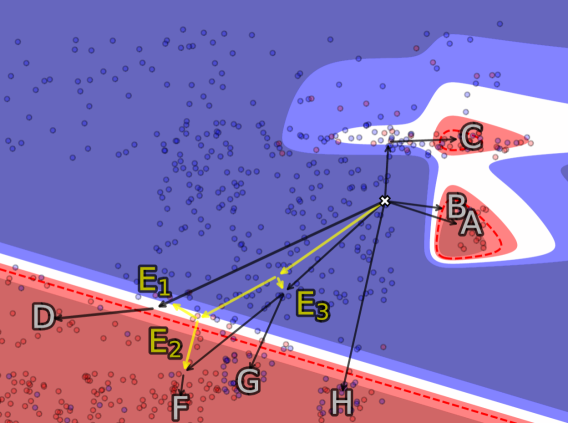
Figure 1: Example of explanatory multiverse constructed for tabular data with two continuous (numerical) features. It shows various types of counterfactual path geometry: their affinity, branching, divergence and convergence. Each journey terminates in a (possibly the same or similar) counterfactual explanation but the characteristics of the steps leading there make some explanations more attractive targets, e.g., by giving the explainee more agency through multiple actionable choices towards the end of a path.

1 Indistinguishability of Counterfactual Paths

Counterfactuals are some of the most popular explanations when faced with unintelligible machine learning (ML) models. Their appeal – both to lay and technical audiences – is grounded in decades of social science research [Miller, 2019] and compliance with various legal frameworks [Wachter et al., 2017]. Fundamentally, counterfactual explanation generation relies on finding an instance whose class is different from the one of the factual data point while minimising the distance between the two – a flexible retrieval process that can be tweaked to satisfy bespoke desiderata.

The increasing popularity of counterfactuals and their highly customisable generation mechanism have encouraged researchers to incorporate sophisticated technical and social requirements into their retrieval algorithms to better reflect their real-life situatedness. Relevant technical aspects include tweaking the fewest possible attributes to guarantee explanation sparsity, or ensuring that counterfactual instances come from a data manifold either by relying on hitherto observed instances [Keane & Smyth, 2020; Poyiadzi et al., 2020; van Looveren & Klaise, 2021] or by constructing them in dense regions [Förster et al., 2021]. Desired social properties reflect real-life constraints embedded in the underlying operational context and data domain, e.g., (im)mutability of certain features, such as date of birth, and directionality of change of others, such as age. The mechanisms employed to retrieve these explanations have evolved accordingly: from techniques that simply output counterfactual instances (accounting for selected social and technical desiderata as part of optimisation) [Wachter et al., 2017; Russell, 2019; Romashov et al., 2022], to methods that construct viable paths between factual and counterfactual points, ensuring feasibility of this journey [Poyiadzi et al., 2020; Downs et al., 2020; Förster et al., 2021; Karimi et al., 2021] (called algorithmic recourse [Ustun et al., 2019]).

All of these properties aid in generating admissible counterfactuals, but they do not offer guidance on how to discriminate between them. Available explainers tend to output multiple counterfactuals whose differences, as it stands, can only be captured through: high-level desiderata, e.g., chronology and coherence; quantitative metrics, e.g., completeness, proximity and neighbourhood density; or qualitative assessment, e.g., user trust and confidence [Sokol & Flach, 2020a; Keane et al., 2021; Small et al., 2023]. In principle, explanation plurality is desirable since it facilitates (interactive) personalisation by offering versatile sets of actions to be taken by the explainees instead of just the most optimal collection of steps (according to a predefined objective), thus catering to unique needs and expectations of diverse audiences [Sokol & Flach, 2018, 2020c]. Nonetheless, this multiplicity is also problematic as without incorporating domain-specific knowledge, collecting user input or relying on generic “goodness” heuristics and criteria [Keane et al., 2021] to filter out redundant explanations – which remains an open challenge – they are likely to overwhelm the explainees.

While comparing counterfactual instances based on their diversity as well as overall feasibility and actionability, among other properties, may inform their pruning, considering the (geometric) relation between the paths leading to them could prove more potent. Current literature treats such paths as independent, thus forgoing any spatial relation between them, whether captured by their direction, length or number of steps (including alignment and size thereof). Additionally, while the feasibility of attribute tweaks, i.e., feature actionability or mutability, is often considered, the direction and magnitude of such changes is largely neglected, e.g., age can only increase at a fixed rate. Modelling such aspects of counterfactual paths is bound to offer domain-independent, spatially-informed heuristics that reduce the number of explanations for users to consider, grant them agency, inform their decision-making and support forward planning.

The role of geometry in (counterfactual) explainability is captured by Figure 1, which demonstrates the diverse characteristics of counterfactual paths for a two-dimensional toy data set with continuous numerical features. When considered in isolation, these paths have the following properties:

A

is short and leads to a high-confidence region, but it lacks data along its journey, which signals infeasibility;

B

while shorter, it terminates close to a decision boundary, thus carries high uncertainty;

C

addresses the shortcomings of A, but it lands in an area of high instability (compared to D, E_i, F, G & H);

G & H

also do not exhibit the deficiencies of A, but they are located in a region with a high error rate;

D & F

have all the desired properties, but they require the most travel; and

E_i

are feasible, but they are incomplete by themselves.

While such considerations have become commonplace in the literature, they treat each destination and path leading to it independently, thus forgoing the benefit of accounting for their spatial relation such as affinity, branching, divergence or convergence. For example, accessing D, F & G via E_i elongates the journey leading to these counterfactuals, making them less attractive based on current desiderata; nonetheless, such a path maximises the agency of explainees by providing them with multiple recourse choices along this trajectory.

Reasoning about the properties of and comparing counterfactual paths is intuitive in two-dimensional spaces – as demonstrated by Figure 1 – but doing so in higher dimensions requires a more principled approach. To this end, we formalise the concept of explanatory multiverse (Section 2), which embraces the multiplicity of counterfactual explanations and captures the geometry, i.e., spatial dependence, of journeys leading to them. Our conceptualisation accounts for technical, spatially-unaware desiderata prevalent in the literature – e.g., plausibility, path length, number of steps, sparsity, magnitude of attribute change and feature actionability – and defines novel, spatially-aware properties such as branching delay, branching factor, (change in) path directionality and affinity between journeys. We propose two possible approaches to embrace explanatory multiverse:

1. vector-based paths, which can rely on data density (model-agnostic) or gradient methods, and are apt for continuous feature spaces (Section 3); and

2. pathfinding in (directed) graphs, which can be built for data based on a predefined distance metric, and is best suited for discrete feature spaces (Section 4).

In addition to imbuing counterfactuals with spatial awareness, explanatory multiverse reduces the number of admissible explanations by collapsing paths based on their affinity and ranking them through our spatially-aware desiderata. We make it easy for others to embark on this novel counterfactuals research journey by releasing a Python package called FACElift that implements our methods.

From the explainees’ perspective, our approach helps them to navigate explanatory multiverse and grants them initiative and agency, empowering meaningful exploration, customisation and personalisation of counterfactuals. For example, by choosing a path recommended based on a high number of diverse explanations accessible along it – refer to segments E_i in Figure 1 – the user is given numerous opportunities to receive the desired outcome while applying a consistent set of changes, thus reducing the number of u-turns and backtracking arising in the process. Explanatory multiverse is also compatible with human-in-the-loop, interactive explainability [Sokol & Flach, 2018, 2020c; Keenan & Sokol, 2023] and a relatively recent decision-support model of explainability, which relies on co-construction of explanations and complements the more ubiquitous “prediction justification” paradigm [Miller, 2023]. We explore and discuss these concepts further in Section 5, before concluding the paper and outlining future work in Section 6.

2 Preliminaries

Before we formalise explanatory multiverse desiderata (Section 2.2), we summarise the notation (Section 2.1) used to introduce our two methods. Throughout this paper we assume that we are given a (state-of-the-art) explainer that generates counterfactuals along with steps leading to them, such as FACE [Poyiadzi et al., 2020] or any algorithmic recourse technique [Ustun et al., 2019; Karimi et al., 2021]. The proposed solutions work with explainers that follow actual data instances and those that operate directly on feature spaces (e.g., by using the density of a data distribution).

2.1 Notation

We denote the $m$-dimensional input space as $\mathcal{X}$, with the explained (factual) instance given by $\mathring{x}$ and the explanation (counterfactual) data point by $\check{x}$. These instances are considered in relation to a predictive model $f:\mathcal{X}\mapsto\mathcal{Y}$, where $\mathcal{Y}$ is the space of possible classes; therefore, $f(\mathring{x})\neq f(\check{x})$ and the prediction of the former data point $f(\mathring{x})=\mathring{y}\in\mathcal{Y}$ is less desirable than that of the latter $f(\check{x})=\check{y}\in\mathcal{Y}$. $\tilde{f}$ refers to the probabilistic realisation of $f$ that outputs the probability of the desired class. Vector $p$-norms, which provide a measurement of length, are defined as $\lVert v\rVert_{p}=\left(\sum_{i=1}^{n}\lvert v_{i}\rvert^{p}\right)^{\frac{1}{p}}$. Distance functions, e.g., on the input space, are denoted by $d:\mathcal{X}\times\mathcal{X}\mapsto\mathbb{R}^{+}$, where the score of $0$ represents identical instances, i.e., $d(x_{a},x_{b})=0\implies x_{a}\equiv x_{b}$, and the higher the score, the more different the data points are.

To discover $\check{x}$ and the steps necessary to transform $\mathring{x}$ into this instance, we apply a state-of-the-art, path-based explainer – see Section 2.2 for the properties expected of it – that generates (multiple) counterfactuals along with their journeys. Each such explanation $Z^{[k]}$ is represented by an $m\times n$ matrix whose $n$ columns $z^{[k]}_{i}\in\mathcal{X}$ capture the sequence of steps in the $m$-dimensional input space, i.e., $Z^{[k]}=[z_{1}^{[k]}\;\cdots\;z_{n}^{[k]}]$, such that if we start at the factual point $\mathring{x}$, we end at the counterfactual instance $\check{x}$ like so: $\check{x}=\mathring{x}+\sum_{i=1}^{n}z_{i}^{[k]}$. For the vector-based explanatory multiverse, each step can be discounted by a weight factor $w_{i}$ that captures its properties, with the weight vector $w=[w_{1}\;\cdots\;w_{n}]$ adhering to the following constraints: $\lVert w\rVert_{2}=1$ and $w_{1}\geq w_{2}\geq\cdots\geq w_{n-1}\geq w_{n}$.

For the graph-based approach, we take $G=(V,E)$ to be a (directed) graph with vertices $V$ and arcs (directed edges) $E$. Each vertex $v_{i}\in V$ corresponds to a data point $x_{i}\in\mathcal{X}$ in the input space, i.e., $v_{i}\equiv x_{i}$; these are connected with (directed) edges $e_{a,b}\in E$ that leave $v_{a}$ and enter $v_{b}$. Assuming that $v_{i}$ represents the explained instance $\mathring{x}$, thus the starting point of a path, and $v_{j}$ is the target counterfactual data point $\check{x}$, thus where the journey terminates, we can identify multiple paths $Z^{[k]}$ connecting them. Here, the columns $z_{i}^{[k]}$ of the $m\times n$ matrix $Z^{[k]}$ representing an $n$-step explanatory journey hold a sequence of vertices $v_{i}$ along this path, i.e., $z_{i}^{[k]}\equiv v_{i}$, with $z_{1}^{[k]}\equiv\mathring{x}$ and $z_{n}^{[k]}\equiv\check{x}$. Such a journey can alternatively be denoted by the corresponding sequence of edges $E_{1,n}=[e_{1,2}\;\cdots\;e_{n-1,n}]\subseteq E$ that encode the properties of each transition (akin to the weights $w_{i}$ used in the vector space approach).

2.2 Desiderata

By using pre-existing, state-of-the-art, path-based explainers, we can retrieve counterfactuals according to the well-known, spatially-unaware desiderata that account for the notions of: (1) distancebetween the explained instance and the explanation [Wachter et al., 2017; Tolomei et al., 2017]; (2) feature (im)mutability or actionability [Ustun et al., 2019; Karimi et al., 2021]; (3) feasibilityof the counterfactual data point [Pawelczyk et al., 2020; Poyiadzi et al., 2020; Downs et al., 2020; van Looveren & Klaise, 2021]; and (4) diversityof the resulting explanations [Mothilal et al., 2020; Keane et al., 2021; Laugel et al., 2023].

The first group includes properties such as the length of a counterfactual path, its number of steps, the number of features being tweaked as well as the magnitude of these individual changes, striving for the smallest possible distance and the minimal number of affected features, i.e., similarity or closeness, and parsimony. The second set accounts for (domain-specific) constraints pertaining to feature alterations; specifically, (im)mutability of attributes, direction and rate of their change as well as their actionability from a user’s perspective (e.g., some tweaks are irreversible, some can be implemented by explainees and others – mutable but non-actionable – are properties of the environment). The third category deals with characteristics of counterfactual data points as well as the intermediate instances that constitute their paths; in particular, we expect them to be feasible according to the underlying data distribution, thus come from the data manifold, enforced either through density constraints or by following pre-existing instances, and of high confidence, i.e., robust, in view of the explained predictive model. The fourth group, which is the least explored, deals with multiplicity of admissible counterfactual explanations; primarily, these are path-agnostic objectives that aim to select a representative subset of instances that are the most diverse and least similar.

We embed our conceptualisation of explanatory multiverse on top of these properties – which it inherits by relying on state-of-the-art, path-based counterfactual explainers – and extend them with three novel, spatially-aware desiderata.

Agency

captures the number of choices – leading to diverse counterfactuals – available to explainees as they traverse explanatory paths. High agency offers a selection of explanations and stimulates user initiative. It can be measured as branching factor, i.e., the number of paths leading to representative explanations accessible at any given step.

Loss of opportunity

encompasses the incompatibility of subsets of explanations that emerges as a consequence of implementing changes prescribed by steps along a counterfactual path. For example, moving towards one explanation may require backtracking the steps taken thus far – which may be impossible due to strict directionality of change imposed on relevant features – to arrive at a different, equally suitable counterfactual. Such a loss of opportunity can be measured by (a decrease in) the proportion of counterfactuals reachable after taking a step without the need of backtracking, which can be quantified by the degree of change in path directionality (vectors) or vertex inaccessibility (graphs).

Choice complexity

encapsulates the influence of explainees’ decisions to follow a specific counterfactual path on the availability of diverse alternative explanations. It can be understood as loss of opportunity accumulated along different explanatory trajectories. For example, among otherwise equivalent paths, following those whose branching is delayed reduces early commitment to a particular set of explanations. It can be measured by the distance (or number of steps and their magnitude) between the factual data point and the earliest consequential point of counterfactual path divergence.

To illustrate the benefits of navigating counterfactuals through the lens of explanatory multiverse, consider a patient who can receive a number of medical treatments. Choosing one of them may preclude others, e.g., due to drug incompatibility – a scenario captured by loss of opportunity. Deciding on medical procedures that are the most universal, thus shared across many therapies, allows to delay the funnelling towards specific courses of treatment – a benefit of accounting for choice complexity. In general, the landscape of available treatments can be more easily navigated by taking actions that do not limit explainees’ choices – a prime example of agency. Notably, we can strive for all of these desiderata simultaneously, weighting some in favour of others if necessary, which we explore further in Section 5.

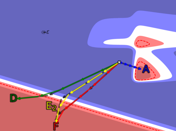
(a) $p=5$ and $\epsilon=0.1$.

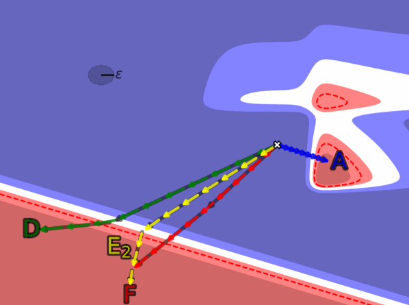
(b) $p=10$ and $\epsilon=0.25$.

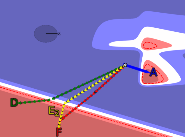
(c) $p=25$ and $\epsilon=0.5$.

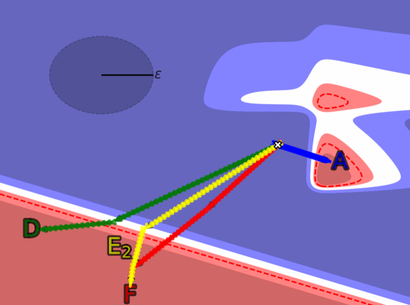
(d) $p=50$ and $\epsilon=1$.

Figure 2: Demonstration of how the number of vectors $p$ into which a path is split and the branching threshold $\epsilon$ affect counterfactual trajectories and branching points. These parameters must be carefully selected, which may require domain knowledge and familiarity with the underlying data; e.g., if $\epsilon\geq 1$, paths E₂ and F are not considered to diverge at any point.

3 Vector Space Interpretation

It should be clear by now that offering each admissible counterfactual as an independent sequence of steps and ordering these explanations purely based on their overall length fails to fully capture some fundamental, human-centred properties, e.g., agency. We must therefore seek strategies to compare the geometry of each counterfactual path, but such a task comes with challenges of its own.

3.1 Comparing Journeys of Varying Length

Counterfactual paths may differ in their overall length, number of steps, individual magnitude thereof and the like. For example, juxtapose paths B and F in Figure 1. The former is built with fewer steps and is much shorter than the latter, making the direct geometrical comparison via their original components infeasible – we could only do so up to the number of steps of the shorter of the two paths (assuming that these steps themselves are of similar length). We address this challenge by comparing counterfactual journeys through their normalised relative sections.

Given two paths $Z^{[a]}\in\mathbb{R}^{m\times n_{1}}$ and $Z^{[b]}\in\mathbb{R}^{m\times n_{2}}$ differing in number of steps, i.e., $n_{1}\neq n_{2}$, we encode them with an equal number of vectors $p$ such that $\bar{Z}^{[a]},\bar{Z}^{[b]}\in\mathbb{R}^{m\times p}$ are normalised journeys. To this end, we define a function

$$c_{L}(Z)=\sum_{i=1}^{n}\lVert z_{i}\rVert_{2}$$

that provides us with the total length of a counterfactual path $Z\in\mathbb{R}^{m\times n}$. We then select the number of steps $p$ into which we partition each journey – these serve as comparison points for paths of differing length. Therefore, the $j$^th step $\bar{z}_{j}$ of a normalised counterfactual journey $\bar{Z}\in\mathbb{R}^{m\times p}$ is

$$\bar{z}_{j}=\sum_{i=1}^{p}\delta_{z_{i}}\left(\frac{j}{p}c_{L}(Z)-\sum_{l=1}^{i}\lVert z_{l}\rVert_{2}\right)z_{i}\text{~{},}$$

where

$$\delta_{z_{i}}(\zeta)=\begin{cases}0\qquad&\text{if}\;\zeta\leq 0\\ \frac{\zeta}{\lVert z_{i}\rVert_{2}}&\text{if}\;0<\zeta\leq\lVert z_{i}\rVert_{2}\\ 1&\text{otherwise}\end{cases}\text{~{}.}$$

This procedure – captured by Algorithm 1 and demonstrated in Figure 2 – allows us to directly compare $\bar{Z}$ with any other path normalised to the same number of steps $p$.

Algorithm 1 Split counterfactual path $Z$ into $p$ vectors.

0   counterfactual path $Z\in\mathbb{R}^{m\times n}$; number of partitions $p\in\mathbb{Z}^{+}$.

0   counterfactual path $\bar{Z}\in\mathbb{R}^{m\times p}$ with $p$ steps.

1   for $j\leftarrow 1$;  $j\leftarrow j+1$;  $j\leq p$ do

2      $\beta\leftarrow\frac{j}{p}c_{L}(Z)$ // split path’s total length

3      $\tau\leftarrow\mathbf{0}$

4      for $i\leftarrow 1$;  $i\leftarrow i+1$;  $i\leq n$ do

5         if $\beta<0$ then

6            continue

7         else if $0\leq\beta\leq\lVert z_{i}\rVert_{2}$ then

8            $\tau\leftarrow\tau+\frac{\beta}{\lVert z_{i}\rVert_{2}}z_{i}$

9         else

10            $\tau\leftarrow\tau+z_{i}$

11         end if

12         $\beta\leftarrow\beta-\lVert z_{i}\rVert_{2}$

13      end for

14      $\bar{z}_{j}\leftarrow\tau$

15   end for

3.2 Identifying Branching Points

We can calculate the proximity between two counterfactual paths $\bar{Z}^{[a]},\bar{Z}^{[b]}\in\mathbb{R}^{m\times p}$ at all points along $\bar{Z}^{[a]}$, therefore find the location of their divergence. To this end, we compute the minimum distance between the path $\bar{Z}^{[b]}$ and the $i$^th point $\bar{z}_{i}^{[a]}$ on the path $\bar{Z}^{[a]}$ with

$$\bar{z}_{i}^{[a|b]}=d_{S}(\bar{Z}^{[b]}-z^{[a]}_{i}\mathbf{1}_{p}^{T})\text{~{},}$$

where

$$d_{S}(Z)=\min_{1\leq j\leq p}\lVert z_{j}\rVert_{2}=\min_{1\leq j\leq p}\sqrt{\sum_{i=1}^{m}\lvert z_{i,j}\rvert^{2}}$$

and $\mathbf{1}_{p}^{T}=[1\;\cdots\;1]$ such that $|\mathbf{1}_{p}|=p$. Next, we define a branching threshold $\epsilon>0$ such that two paths are considered to have separated at a divergence point $p^{\star}$ where $\bar{z}_{i}^{[a|b]}$ first exceeds the threshold $\epsilon$, i.e., $p^{\star}=\min(i)$ s.t. $\bar{z}_{i}^{[a|b]}>\epsilon$. We can then denote the proportion along the journey $\bar{Z}^{[a]}$ before it branches away from $\bar{Z}^{[b]}$ as $\frac{p^{\star}-1}{p}$. This procedure is captured by Algorithm 2 and demonstrated in Figure 2.

Algorithm 2 Identify branching point $p^{\star}$.

0   normalised counterfactual paths $\bar{Z}^{[a]},\bar{Z}^{[b]}\in\mathbb{R}^{m\times p}$; branching threshold $\epsilon>0$.

0   divergence point $p^{\star}$.

1   for $i\leftarrow 1$;  $i\leftarrow i+1$;  $i\leq p$ do

2      if $\bar{z}_{i}^{[a|b]}>\epsilon$ then

3         $p^{\star}\leftarrow i$

4         break

5      end if

6   end for

3.3 Direction Difference Between Paths

After normalising two counterfactual paths to have the same number of steps, i.e., $\bar{Z}^{[a]},\bar{Z}^{[b]}\in\mathbb{R}^{m\times p}$, we can compute direction difference between them. Popular distance metrics, e.g., the Euclidean norm, can be adapted to this end:

$$d_{E}(\bar{Z}^{[a]},\bar{Z}^{[b]}) =\sum_{j=1}^{p}w_{i}\rVert\bar{z}^{[a]}_{i,j}-\bar{z}^{[b]}_{i,j}\rVert_{2}$$

$$=\sum_{j=1}^{p}w_{i}\sqrt{\sum_{i=1}^{m}(\bar{z}^{[a]}_{i,j}-\bar{z}^{[b]}_{i,j})^{2}}\text{~{},}$$

where $d_{E}:Z\times Z\mapsto\mathbb{R}^{+}$ and the weight vector $w$, with $|w|=p$, is as outlined in Section 2.1. $d_{E}$ therefore offers a measure of directional separation between two journeys such that $d_{E}(\bar{Z}^{[a]},\bar{Z}^{[b]})=0\implies\bar{Z}^{[a]}\equiv\bar{Z}^{[b]}$, and $d_{E}(\bar{Z}^{[a]},\bar{Z}^{[b]})<d_{E}(\bar{Z}^{[a]},\bar{Z}^{[c]})$ implies that $\bar{Z}^{[a]}$ is more similar to $\bar{Z}^{[b]}$ than to $\bar{Z}^{[c]}$.

4 Directed Graph Interpretation

Applying changes to one’s situation to achieve the desired outcome is an inherently continuous and incremental process [Barocas et al., 2020]. Given the extended period of time it can span, this process may fail or be abandoned, e.g., due to an unexpected change in circumstances, thus it may require devising alternative routes to the envisaged outcome. However, some of the actions taken thus far may make the adaptation to the new situation difficult or even impossible, prompting us to consider the loss of opportunity resulting from counterfactual path branching. To this end, explanatory multiverse extends the concept of counterfactual paths by accounting for uni-directional changes of features that reflect their monotonicity (as well as immutability) and recognising feature tweaks that cannot be undone. Our directed graph implementation – see Algorithm 3 – builds upon FACE [Poyiadzi et al., 2020] by extending its $k$-nearest neighbours ($k$-NN) approach that generates counterfactuals with the shortest path algorithm [Dijkstra, 2022].

4.1 Branching

Let $r_{i}$ denote the branching factor of a node $v_{i}$, and $r_{a,b}$ be the branching factor of a path $E_{a,b}$ between nodes $v_{a}$ and $v_{b}$ consisting of $p$ steps. $r_{i}$ can be defined as the average of the shortest distance from the vertex $v_{i}$ to each accessible node of the counterfactual class, or of all alternative classes for multi-class classification; its formulation depends on the data set and problem domain (a specific example is provided in Section 4.2). The number of candidate points can be reduced by introducing diversity criteria, e.g., (absolute) feature value differences, thus considering only a few representative counterfactuals. $r_{a,b}$ is defined as the average of individual branching factors $r_{i}$ corresponding to vertices $v_{i}$ that are travelled through when following the edges $e_{i,i+1}$ of the counterfactual path $E_{a,b}$, and computed as

$$r_{a,b}=\frac{1}{p-2}\sum_{i=1}^{p-1}r_{i}\text{~{}.}$$

The first and last nodes are excluded since the former is shared among all the paths and we stop exploring beyond the latter. To account for choice complexity, we can introduce a discount factor $\gamma\in\mathbb{R}^{+}$ that allows us to reward ($\gamma>1$) or penalise ($\gamma<1$) branching in the early stages of a path:

$$r_{a,b}=\frac{1}{p-2}\sum_{i=1}^{p-1}\gamma^{i-1}r_{i}\text{~{}.}$$

Algorithm 3 Build graph-based explanatory multiverse.

0   data set $X$; probabilistic model $\tilde{f}$; instance to be explained $\mathring{x}$; neighbours number $k$; counterfactual classification threshold $t$.

0   directed data graph $G=(V,E)$; candidate counterfactuals $\check{X}$; branching factor of paths $R$.

1   for every pair $(x_{i},x_{j})\in X$ do // build graph

2      $e_{i,j}\leftarrow d(x_{i},x_{j})$ // compute distance

3   end for

4   $V\leftarrow X$

5   $E\leftarrow\mathit{prune}$(E, k) // keep $k$-NN for each node

6   $x_{i}\equiv\mathring{x}$

7   for $x_{j}\in X$ do

8      if $\tilde{f}(x_{j})\geq t$ then

9         $\check{X}\leftarrow\check{X}\cup x_{j}$

10         $E_{i,j}\leftarrow\mathit{dijkstra}(G,x_{i},x_{j})$ // shortest path

11         $r_{i,j}\leftarrow\mathit{branching}(G,E_{i,j})$

12         $R\leftarrow R\cup r_{i,j}$

13      end if

14   end for

4.2 Constraining Feature Changes

Our directed graph approach implements feature monotonicity to capture uni-directional changes of relevant attribute values. For some data domains, however, imposing such a strict assumption may be too restrictive and yield no viable explanations, as is the case in our next example – path-based counterfactuals for the MNIST data set of handwritten digits [LeCun, 1998]. Here, the explanations capture (step-by-step) transitions between different digits, which process is realised through addition of individual pixels; the plausibility of such paths is enforced by composing them exclusively of instances observed before (and stored in a dedicated data set). As noted, such a restrictive setup yields no viable counterfactual paths, which prompts us to relax the feature monotonicity constraint by allowing pixels to be removed; we specify this action to be $\lambda$ times more difficult than adding pixels, where $\lambda\in\mathbb{R}^{+}$ is a penalty term. This formalisation simulates scenarios where backtracking steps of a counterfactual path is undesirable, which in the case of MNIST can be viewed as removing pixels that are already in an image (whether pre-existing or added during recourse). The corresponding distance between two nodes $v_{a}$ and $v_{b}$ can be defined as

$$d_{\lambda}(v_{a},v_{b})=\sqrt{\sum_{i=1}^{m}\left(\phi_{\lambda}(v_{a,i},v_{b,i})(v_{a,i}-v_{b,i})\right)^{2}}\text{~{},}$$

where $v_{a,i}$ is the $i$^th feature of $x_{a}$ represented by $v_{a}$ and

$$\phi_{\lambda}(v_{a,i},v_{b,i})=\begin{cases}-\lambda&\quad\text{if}\;v_{a,i}-v_{b,i}<0\\ 1&\quad\text{otherwise}\end{cases}\text{~{}.}$$

We apply Algorithm 3 with $k=20$ using $d_{\lambda}$ as the distance function, setting $\lambda=1.1$. Figure 3 shows example counterfactual paths starting at $f(\mathring{x})=1$ and terminating at $f(\check{x})=9$. The branching factor of a node $v_{i}$ representing a digit image is computed as $r_{i}=-\log(c(v_{i}))$ for

$$c(v_{i})=\frac{1}{\lvert\mathcal{Y}^{\prime}\rvert}\sum_{y\in\mathcal{Y}^{\prime}}\sum_{e_{m,n}\in E_{a,b}}d_{\lambda}(v_{m},v_{n})\;\;\;\text{s.t.}\;\;\;f(v_{b})=y\text{~{}.}$$

Here, $\mathcal{Y}^{\prime}\equiv\mathcal{Y}\setminus(\mathring{y},\check{y},f(v_{a}))$, i.e., we exclude the factual and counterfactual classes as well as $f(v_{a})$ if $v_{a}$ is an intermediate step; $E_{a,b}$ is the shortest path from $v_{a}$ to nodes $v_{b}$ that represent counterfactual instances, i.e., $f(v_{b})\in\mathcal{Y}^{\prime}$. The path length indicates the number of pixels changed when transforming a factual data point into a counterfactual instance. Branching factor of a path can be interpreted as the ease of switching to alternative paths (higher is better).

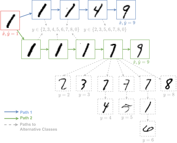
Figure 3: Example counterfactual journeys identified in the MNIST data set of handwritten digits. Paths 1 (blue) and 2 (green) explain an instance $\mathring{x}$ classified as $\mathring{y}=1$ for the counterfactual class $\check{y}=9$. Paths leading to alternative classification outcomes are also possible (shown in grey). Path 1 is shorter than Path 2 at the expense of explainees’ agency – which is reflected in its smaller branching factor – therefore switching to alternative paths leading to different classes is harder, i.e., more costly in terms of distance.

5 Discussion

Explanatory multiverse is a novel conceptualisation of step-based counterfactual explanations (overviewed in Section 1) that inherits all of their desired, spatially-unaware properties and extends them with a collection of spatially-aware desiderata that take advantage of the geometry of counterfactual paths (covered in Section 2.2). Despite being overlooked in the technical literature, such a view on counterfactual reasoning, explainability and decision-making is largely consistent with their account in philosophy, psychology and cognitive science [Kahneman, 2014; Mueller et al., 2021]. Lewis’ [1973] notion of possible-worlds, of which the real world is just one and with some being closer to reality (i.e., more realistic) than others [Kahneman & Varey, 1990], is akin to the numerous interrelated paths connecting a factual instance with counterfactual explanations captured by our formalisation of explanatory multiverse. Specifically, it accounts for spatial and temporal contiguity, thus supports and better aligns with mental simulation, which is a form of automatic and elaborative (counterfactual) thinking. This process spans continuum rather than a typology and allows humans to imagine congruent links between two possible states of the world, e.g., factual and counterfactual, by unfolding a sequence of events connecting them.

Navigating the nexus of (hypothetical) possibilities through the (technical) proxy of explanatory multiverse enables structured – and possibly guided – exploration, comparison and reasoning over (remote branches of) counterfactual explanations. By accounting for the spatial and temporal aspects of their paths – such as affinity, branching, divergence and convergence – we construct an explainability framework capable of modelling a perceptual distance between counterfactual trajectories. For example, it allows us to consider people’s tendency to first undo the changes implemented at the beginning of a process and their propensity to fall prey to the sunk cost fallacy, i.e., continuing an endeavour after the initial effort [Arkes & Blumer, 1985]. To the best of our knowledge, we are the first to model the geometry of explanations, thus better align ML interpretability with modes of counterfactual thinking found in humans.

Explanatory multiverse also advances the human-centred explainability agenda on multiple fronts. It comes with an inherent heuristic to deal with counterfactual multiplicity by recognising their spatial (dis)similarity, thus reducing the cognitive load required of explainees. By lowering the choice complexity when deciding on actions to take while navigating and traversing step-based counterfactual paths, explanatory multiverse better aligns this process with iterative and interactive, dialogue-based, conversational explainability – a process that is second nature to humans [Miller, 2019; Keenan & Sokol, 2023]. Given the ability to consider the general direction of representative counterfactual paths instead of their specific instantiations, which may be overwhelming due to their quantity and lack of meaningful differentiation, our conceptualisation is compatible with both the well-established justification as well as the more recent decision-support paradigms of explainable ML [Miller, 2023]. An additional benefit of explanatory multiverse is its ability to uncover disparity in access to counterfactual recourse – a fairness perspective; some individuals may only be offered a limited set of explanations, or none at all, if they belong to remote clusters of points, e.g., portraying a protected group that is underrepresented in the data.

The three preliminary desiderata outlined in Section 2.2 are general enough to encompass most applications of explanatory multiverse, nonetheless they are far from exhaustive; we envisage identifying more properties as we explore this concept further and apply it to specific problems. Doing so will allow us to learn about their various trade-offs, especially since we expect different data domains and modelling problems to prioritise distinct desiderata. Forgoing naïve optimisation for the shortest path in favour of a deliberate detour can benefit explainees on multiple levels as argued throughout this paper. Some of these considerations can be communicated through intuitive visualisations, making them more accessible (to a lay audience); e.g., we may plot the number of implemented changes against the proportion of counterfactual recourse opportunities that remain available at any given point.

With the current set of properties, for example, one may prefer delayed branching, which incurs small loss of opportunity early on but a large one at later stages, thus initially preserving high agency. Similarly, a small loss of opportunity early on can be accepted to facilitate delayed branching, hence reduce overall choice complexity at the expense of agency. If, in contrast, early branching is desired – e.g., one prefers a medical diagnosis route with fewer required tests – this will result in a large loss of opportunity at the beginning, thus lower agency. Additionally, certain paths may be easier to follow, i.e., preferred, due to domain-specific properties, e.g., a non-invasive medical examination, whereas others may require crossing points of no return, i.e., implementing changes that cannot be (easily) undone.

In view of the promising results offered by our initial experiments, streamlining and extending both of our approaches as well as implementing their variations (e.g., vector paths based on gradient methods) are the next steps, which will allow us to transition away from toy examples and apply our tools to real-life data sets. The vector interpretation of explanatory multiverse is best suited for continuous spaces for which we have a sizeable and representative sample of data. The (directed) graph perspective, on the other hand, is more appropriate for sparse data sets with discrete attributes. Both solutions are intrinsically compatible with multi-class counterfactuals [Sokol & Flach, 2020b] – refer back to the MNIST example shown in Figure 3 – which offer a nuanced and comprehensive explanatory perspective. Note that an action may have multiple distinct consequences: make certain outcomes more likely (or simply possible), others less likely (or even impossible), or both at the same time; therefore, depending on the point of view, each step taken by an explainee can be interpreted as a negative or positive (counterfactual) explanation. Our solutions also facilitate retrospective explanations that allow to (mentally) backtrack steps leading to the current situation – in contrast to prospective explanations that prescribe actionable insights – thus answering questions such as: “How did I end up here?”

6 Conclusion and Future Work

In this paper we introduced explanatory multiverse: a novel conceptualisation of counterfactual explainability that takes advantage of geometrical relation – affinity, branching, divergence and convergence – between paths representing the steps connecting factual and counterfactual data points. Our approach better aligns such explanations with human needs and expectations by distilling informative, intuitive and actionable insights from, otherwise overwhelming, counterfactual multiplicity; explanatory multiverse is also compatible with iterative and interactive explanatory protocols, which are one of the tenets of human-centred explainability.

To guide the retrieval of high-quality explanations, we formalised three spatially-aware desiderata: agency, loss of opportunity and choice complexity; nonetheless, this is just a preliminary and non-exhaustive set of properties, which we expect to expand as we explore explanatory multiverse further and apply it to specific data domains. In addition to foundational and theoretical contributions, we also proposed and implemented two algorithms – one based on vector spaces and the other on (directed) graphs – which we examined across two toy examples – respectively a synthetic, two-dimensional tabular data set and the MNIST hand-written digits – to demonstrate the capabilities of our approach. Our methods, the open source implementation of which is available on GitHub to promote reproducibility, are built upon state-of-the-art, step-based counterfactual explainers, such as algorithmic recourse, therefore they come equipped with all the desired, spatially-unaware properties.

By introducing and formalising explanatory multiverse we have laid the foundation necessary for further exploration of this concept. In addition to advancing our two methods, in future work we will study building dynamical systems, phase spaces and vector fields from (partial) sequences of observations to capture complex dynamics such as divergence, turbulence, stability and vorticity within explanatory multiverse, which appears suitable for medical data such as electronic health records. We will also look into explanation representativeness – i.e., identifying and grouping counterfactuals that are the most diverse and least alike – given that it is central to navigating the geometry of counterfactual paths yet largely under-explored. Discovering (dis)similarity of counterfactuals can streamline the exploration of explanatory multiverse, whether with graphs or vectors, helping to identify pockets of highly attractive or inaccessible explanations; understanding these dependencies is also important given their fairness ramifications as some individuals may only have limited recourse options.

Authors’ Contributions

Conceptualisation: Kacper Sokol (lead investigator), Edward Small, Yueqing Xuan. Methodology: Kacper Sokol (explanatory multiverse), Edward Small (vector-based approach), Yueqing Xuan (graph-based approach). Code development: Edward Small (vector-based approach), Yueqing Xuan (graph-based approach). Writing: Kacper Sokol (explanatory multiverse), Edward Small (vector-based approach), Yueqing Xuan (graph-based approach). Review and editing: Kacper Sokol.

References

- Arkes & Blumer [1985] Arkes, H. R. and Blumer, C. The psychology of sunk cost. Organizational behavior and human decision processes, 35(1):124–140, 1985.
- Barocas et al. [2020] Barocas, S., Selbst, A. D., and Raghavan, M. The hidden assumptions behind counterfactual explanations and principal reasons. In Proceedings of the 2020 conference on fairness, accountability, and transparency, pp. 80–89, 2020.
- Dijkstra [2022] Dijkstra, E. W. A note on two problems in connexion with graphs. In Edsger Wybe Dijkstra: His Life, Work, and Legacy, pp. 287–290. 2022.
- Downs et al. [2020] Downs, M., Chu, J. L., Yacoby, Y., Doshi-Velez, F., and Pan, W. CRUDS: Counterfactual recourse using disentangled subspaces. ICML WHI, 2020:1–23, 2020.
- Förster et al. [2021] Förster, M., Hühn, P., Klier, M., and Kluge, K. Capturing users’ reality: A novel approach to generate coherent counterfactual explanations. 2021.
- Kahneman [2014] Kahneman, D. Varieties of counterfactual thinking. In What might have been, pp. 387–408. Psychology Press, 2014.
- Kahneman & Varey [1990] Kahneman, D. and Varey, C. A. Propensities and counterfactuals: The loser that almost won. Journal of Personality and Social Psychology, 59(6):1101, 1990.
- Karimi et al. [2021] Karimi, A., Schölkopf, B., and Valera, I. Algorithmic recourse: From counterfactual explanations to interventions. In Proceedings of the 2021 ACM conference on fairness, accountability, and transparency, pp. 353–362, 2021.
- Keane & Smyth [2020] Keane, M. T. and Smyth, B. Good counterfactuals and where to find them: A case-based technique for generating counterfactuals for explainable AI (XAI). In Case-Based Reasoning Research and Development: 28th International Conference, ICCBR 2020, Salamanca, Spain, June 8–12, 2020, Proceedings 28, pp. 163–178. Springer, 2020.
- Keane et al. [2021] Keane, M. T., Kenny, E. M., Delaney, E., and Smyth, B. If only we had better counterfactual explanations: Five key deficits to rectify in the evaluation of counterfactual XAI techniques. In IJCAI, pp. 4466–4474, 2021.
- Keenan & Sokol [2023] Keenan, B. and Sokol, K. Mind the gap! Bridging explainable artificial intelligence and human understanding with Luhmann’s functional theory of communication. arXiv preprint arXiv:2302.03460, 2023.
- Laugel et al. [2023] Laugel, T., Jeyasothy, A., Lesot, M.-J., Marsala, C., and Detyniecki, M. Achieving diversity in counterfactual explanations: A review and discussion. In Proceedings of the 2023 ACM conference on fairness, accountability, and transparency, pp. 1859–1869, 2023.
- LeCun [1998] LeCun, Y. The MNIST database of handwritten digits. http://yann.lecun.com/exdb/mnist/, 1998.
- Lewis [1973] Lewis, D. Counterfactuals. Harvard University Press, Cambridge, Massachusetts, 1973.
- Miller [2019] Miller, T. Explanation in artificial intelligence: Insights from the social sciences. Artificial Intelligence, 267:1–38, 2019.
- Miller [2023] Miller, T. Explainable AI is dead, long live explainable AI! Hypothesis-driven decision support using evaluative AI. In Proceedings of the 2023 ACM conference on fairness, accountability, and transparency, pp. 333–342, 2023.
- Mothilal et al. [2020] Mothilal, R. K., Sharma, A., and Tan, C. Explaining machine learning classifiers through diverse counterfactual explanations. In Proceedings of the 2020 conference on fairness, accountability, and transparency, pp. 607–617, 2020.
- Mueller et al. [2021] Mueller, S. T., Veinott, E. S., Hoffman, R. R., Klein, G., Alam, L., Mamun, T., and Clancey, W. J. Principles of explanation in human–AI systems. AAAI 2021 Workshop on explainable agency in artificial intelligence, 2021.
- Pawelczyk et al. [2020] Pawelczyk, M., Broelemann, K., and Kasneci, G. Learning model-agnostic counterfactual explanations for tabular data. In Proceedings of the 2020 web conference, pp. 3126–3132, 2020.
- Poyiadzi et al. [2020] Poyiadzi, R., Sokol, K., Santos-Rodriguez, R., De Bie, T., and Flach, P. FACE: Feasible and actionable counterfactual explanations. In Proceedings of the AAAI/ACM conference on AI, ethics, and society, pp. 344–350, 2020.
- Romashov et al. [2022] Romashov, P., Gjoreski, M., Sokol, K., Martinez, M. V., and Langheinrich, M. BayCon: Model-agnostic Bayesian counterfactual generator. In IJCAI, pp. 740–746, 2022.
- Russell [2019] Russell, C. Efficient search for diverse coherent explanations. In Proceedings of the 2019 conference on fairness, accountability, and transparency, pp. 20–28, 2019.
- Small et al. [2023] Small, E., Xuan, Y., Hettiachchi, D., and Sokol, K. Helpful, misleading or confusing: How humans perceive fundamental building blocks of artificial intelligence explanations. ACM CHI 2023 workshop on human-centered explainable AI (HCXAI), 2023.
- Sokol & Flach [2018] Sokol, K. and Flach, P. Glass-Box: Explaining AI decisions with counterfactual statements through conversation with a voice-enabled virtual assistant. In IJCAI, pp. 5868–5870, 2018.
- Sokol & Flach [2020a] Sokol, K. and Flach, P. Explainability fact sheets: A framework for systematic assessment of explainable approaches. In Proceedings of the 2020 conference on fairness, accountability, and transparency, pp. 56–67, 2020a.
- Sokol & Flach [2020b] Sokol, K. and Flach, P. LIMEtree: Consistent and faithful surrogate explanations of multiple classes. arXiv preprint arXiv:2005.01427, 2020b.
- Sokol & Flach [2020c] Sokol, K. and Flach, P. One explanation does not fit all. KI-Künstliche Intelligenz, pp. 1–16, 2020c.
- Tolomei et al. [2017] Tolomei, G., Silvestri, F., Haines, A., and Lalmas, M. Interpretable predictions of tree-based ensembles via actionable feature tweaking. In Proceedings of the 23rd ACM SIGKDD international conference on knowledge discovery and data mining, pp. 465–474, 2017.
- Ustun et al. [2019] Ustun, B., Spangher, A., and Liu, Y. Actionable recourse in linear classification. In Proceedings of the 2019 conference on fairness, accountability, and transparency, pp. 10–19, 2019.
- van Looveren & Klaise [2021] van Looveren, A. and Klaise, J. Interpretable counterfactual explanations guided by prototypes. In Machine Learning and Knowledge Discovery in Databases. Research Track: European Conference, ECML PKDD 2021, Bilbao, Spain, September 13–17, 2021, Proceedings, Part II 21, pp. 650–665. Springer, 2021.
- Wachter et al. [2017] Wachter, S., Mittelstadt, B., and Russell, C. Counterfactual explanations without opening the black box: Automated decisions and the GPDR. Harv. JL & Tech., 31:841, 2017.