EffCRN: An Efficient Convolutional Recurrent Network
for High-Performance Speech Enhancement

Abstract

Fully convolutional recurrent neural networks (FCRNs) have shown state-of-the-art performance in single-channel speech enhancement. However, the number of parameters and the FLOPs/second of the original FCRN are restrictively high. A further important class of efficient networks is the CRUSE topology, serving as reference in our work. By applying a number of topological changes at once, we propose both an efficient FCRN (FCRN15), and a new family of efficient convolutional recurrent neural networks (EffCRN23, EffCRN23lite). We show that our FCRN15 (875K parameters) and EffCRN23lite (396K) outperform the already efficient CRUSE5 (85M) and CRUSE4 (7.2M) networks, respectively, w.r.t. PESQ, DNSMOS and $\Delta$SNR, while requiring about 94% less parameters and about 20% less #FLOPs/frame. Thereby, according to these metrics, the FCRN/EffCRN class of networks provides new best-in-class network topologies for speech enhancement.

Index Terms: noise suppression, efficient networks, convolutional recurrent neural networks, speech enhancement

1 Introduction

In single channel noise suppression the aim is to estimate a clean speech signal from a noisy mixture of clean speech and interfering background noise. For real world applications, efficient methods enabling low-latency real-time processing and adhering to memory limitations are of utmost importance [1, 2, 3, 4]. Recently, neural networks have seen increasing use for this task with many of the prominent approaches estimating a complex spectral mask for the noisy speech in the short-time Fourier transform (STFT) domain [5, 6, 7, 8].

Especially convolutional neural networks (CNNs) have been widely used for the task of speech enhancement [9, 10, 11]. The sliding kernels allow for precise modelling of local dependencies in the speech spectra [10].

Recurrent processing has been employed to model temporal dependencies in addition to spectral characteristics [12]. Namely, long short-term memory (LSTM) [13] and gated recurrent unit (GRU) [14] layers have been incorporated into CNNs [15, 16]. A fully convolutional recurrent network (FCRN) [10] has been introduced to combine the strengths of convolutional modelling even throughout the recurrent layers by using convolutional LSTMs (CLSTMs) for feature processing, achieving state-of-the-art performance [6].

Considering the reduction of computational complexity, multiple approaches such as pruning or quantization have been proposed [3, 1]. Earlier models achieved efficiency using hybrid processing methods and coarse features [4] while recent methods employed deep filtering in a multi-stage setup [17]. While other fields have seen neural architecture search employed to find efficient base topologies for subsequent scaling [18], in speech enhancement an important recent advancement in terms of providing an efficient high-performance topology was the Convolutional Recurrent U-net for Speech Enhancement (CRUSE) class of networks [2]. However, the reduction of computational complexity comes with a tradeoff in terms of model performance. Additionally, the huge parameter counts, with the smaller CRUSE versions being even in the range of the original FCRN ($5.2$ M) or higher, remain a problem for memory-constrained applications.

Our work builds upon the idea of the FCRN and improves the efficiency by reducing the number of filters and the kernel size. This allows to increase the network's depth, but requires to introduce learnable skip connections and an only linear increase (decrease) of filter numbers in the encoder (decoder), thereby creating a smaller network that retains most of its performance. Besides the efficient FCRN15, our core contribution in this paper is the efficient convolutional recurrent neural network (EffCRN) topology which takes the design principles "deeper and wider with smaller kernels" a step further. Additionally, we reduce zero-padding of layer inputs and regain good quality by allowing for non-convolutional layers in the now sparse bottleneck. We compare the FCRN and EffCRN variants to the strongest CRUSE networks.

The paper is structured as follows. Section 2 introduces the evaluation framework and the network topologies used in our experiments. Experimental setup, datasets, and training parameters are detailed in Section 3, followed by a discussion of our experimental results. We conclude in Section 4.

2 Model Topologies

2.1 Evaluation Framework

Our models operate in the STFT domain. The spectral coefficients of clean speech $S_{\ell}(k)$ and noise $D_{\ell}(k)$ yield noisy speech $Y_{\ell}(k)=S_{\ell}(k)+D_{\ell}(k).$ While $\ell$ denotes the frame index, $k\in\mathcal{K}=\{0,1,\dots\allowbreak K\!-\!1\}$ is the frequency bin index of a $K$-point DFT. The models predict a spectral mask $G_{\ell}(k)\in\mathbb{C}$ which is the complex-valued representation of the real-valued network output tensor $\mathbf{G}_{\ell}(k)\in\mathbb{R}^{2}$. The clean speech estimate is then $\hat{S}_{\ell}(k)=G_{\ell}(k)\cdot Y_{\ell}(k)$.

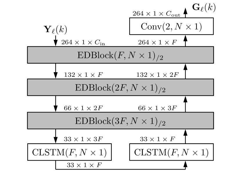
Figure 1: The FCRN15 topology depicted using the EDBlock() detailed in Fig. 2

2.2 FCRN Variants

The original FCRN [6] consists of $10$ convolutional layers, $1$ CLSTM and multiple up-/downsampling layers as well as $2$ skip connections that additively combine features from the encoder and from the decoder. A more efficient version of this network is the FCRN15 depicted in Fig. 1. It performs up- and downsampling with strided convolutions (as shown to be beneficial in [19]) and increases the network's depth to $15$ layers. Additionally, it enhances the additive skip connections with $1\times 1$ depthwise convolutions. Less and smaller filter-kernels enable its two CLSTMs to be more efficient than the FCRN's single CLSTM. We depict the FCRN15 using an encoder-decoder block EDBlock() which combines two convolutions from both encoder and decoder and the learnable skip connections as shown in Fig. 2. It requires two input signals $\mathbf{x}^{\mathrm{enc/dec}}_{\mathrm{in}}$ and produces two output signals $\mathbf{x}^{\mathrm{enc/dec}}_{\mathrm{out}}$. The number of filter kernels is $i\cdot F$, where $i$ is the index of the EDBlock, $N$ and $V=1$ are the size of the 3D kernel along the frequency and the time axis, respectively, and $S=2$ denotes the stride. All employed non-depthwise convolutions possess kernels with a third axis covering all available feature maps. The size of the compressed frequency axis is $M^{\prime}$, while $C_{\mathrm{in}}^{\mathrm{enc/dec}}$ describes the number of channels of each input. Convolutional layers are denoted by $\mathrm{Conv}(i\cdot F,N\times V)_{/S}$, with $S$ being an optional stride. $\mathrm{DeConv}(i\cdot F,N\times V)_{S}$ refers to a transposed convolution with the same parameter set. Layer outputs have a size feature axis $\times$ time axis $\times$ feature maps. In comparison to the well known CRUSE topology we only downsample every other convolutional layer and we increase the number of filters linearly instead of exponentially with depth.

All models take an input $M\times 1\times C_{\mathrm{in}}$ with $M=K/2+1+P$ and $P$ being the number of zeros padded to the non-redundant bins of the spectrum. We use the LeakyReLU activation [20] for all but the last convolutional layer, which uses linear activation. Instead of $G_{\ell}(k)$, the bounded network output

$$G^{\prime}_{\ell}(k)=\mathrm{tanh}(|G_{\ell}(k)|)\cdot\frac{G_{\ell}(k)}{|G_{\ell}(k)|}$$ (1)

with constrained magnitude $|G^{\prime}_{\ell}(k)|\in[0,1]$ is then used for masking by $\hat{S}_{\ell}(k)=G^{\prime}_{\ell}(k)\cdot Y_{\ell}(k)$ [6]. CLSTM activations are tanh and sigmoid as published in [21].

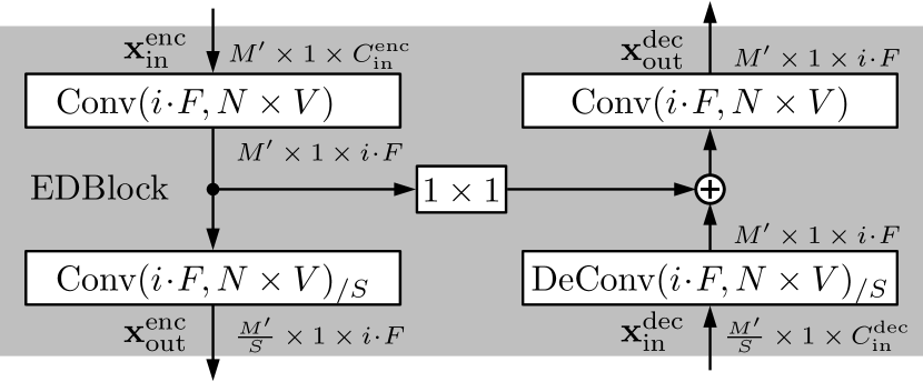
Figure 2: Details of the $i$-th $\mathrm{EDBlock}(i\cdot F,N\times V)_{/S}$, consisting of four convolutional layers, providing downsampling on the encoder side and upsampling on the decoder side.

2.3 The New EffCRN Topologies

The new EffCRN23 topology can also be depicted using the EDBlocks as shown in Figure 3 with an increased total depth of now $23$ layers (change \raisebox{-0.5pt}{\scriptsizeD}⃝). Compared to the FCRN15, the self-evident approach for the EffCRN23 is to initially use fewer and overall significantly smaller filter kernels (change \raisebox{-0.5pt}{\scriptsizeF}⃝). However, contrary to the CRUSE approach, we do not decrease network depth to obtain the smaller network. Instead we increase network depth, thereby allowing the network to compensate for the drastic impact of reduced filter count and size on it's capacity. The increased depth allows the network to find its own powerful feature representation while maintaining overall computing costs low. This is in line with literature which states that an optimal ratio of depth to width exists for a given network [18]. Our network performs further downsampling along the frequency axis and achieves a significantly smaller feature representation at the bottleneck between encoder and decoder, where recurrent modelling takes place. Notably we use the first CLSTM to sharply reduce the number of filters as well for efficient processing. However, to keep output signal quality high, the resulting smaller representation not only allows but requires non-convolutional recurrent bottleneck processing, replacing the second CLSTM layer (change \raisebox{-0.5pt}{\scriptsizeC}⃝) with an efficient non-convolutional GRU layer (change \raisebox{-0.5pt}{\scriptsizeG}⃝) without an excessive increase of model parameters.

Additionally, we reduce computations by optimizing zero-padding and apply it only when necessary (change \raisebox{-0.5pt}{\scriptsizeP}⃝). Single entries are padded to even input sizes in the encoder directly before EDBlocks and the extra entries are removed at the respective location in the decoder as shown in Fig. 3. The EffCRN23lite is an even smaller version of the same topology featuring fewer filters. Activations and output bounding (1) are identical to the FCRN variants.

Please note that the changes from FCRN15 to EffCRN23 can be concisely stated by the introduced shorthand as: $\texttt{EffCRN23}=\texttt{FCRN15}\raisebox{0.0pt}{\scriptsize{+}}\raisebox{-0.5pt}{\scriptsizeD}⃝\raisebox{0.0pt}{\scriptsize{+}}\raisebox{-0.5pt}{\scriptsizeP}⃝\raisebox{0.0pt}{\scriptsize{+}}\raisebox{-0.5pt}{\scriptsizeF}⃝\raisebox{0.0pt}{\scriptsize{-}}\raisebox{-0.5pt}{\scriptsizeC}⃝\raisebox{0.0pt}{\scriptsize{+}}\raisebox{-0.5pt}{\scriptsizeG}⃝$.

2.4 CRUSE Network Baselines

We compare our work against the CRUSE networks [2], which have been designed to be efficient. We choose the two most powerful architectures from [2], namely CRUSE5_256-_2xLSTM1 (CRUSE5) and CRUSE4_128_1xGRU4_convskip (CRUSE4) for re-implementation and reference. They feature a symmetrical encoder-decoder structure consisting entirely of convolutional blocks using a $(3\times 2)$ kernel, whereas our models process single frames $(V=1)$. In the bottleneck they feature either $2$ sequential LSTMs or $4$ parallel GRU layers. The GRUs were fed by flattening, then splitting the input data to those layers. Since we focus on a network comparison, we employ the CRUSE topologies detailed in [2], keeping layers and activations unchanged. Note that applying a linear output layer and a bounding (1) as in the FCRN/EffCRN variants, performance changes negligibly. We use the same input features as for our networks and pad them to fulfill divisibility constraints imposed by repeated downsampling.

3 Experiments and Discussion

3.1 Datasets and Parameter Settings

Experiments are performed on WSJ0 speech data [22] mixed with noise from the DEMAND [23] and QUT [24] datasets for training and development, whereas unseen noise data is taken from the ETSI dataset [25] for the test set. SNR conditions are $0$, $5$ and $10$ dB at an active speech level of $-26$ dBov before mixing [26]. We employ $105$ hours of training data, $10$ hours of validation data, and 1 hour of test data, with disjoint speakers between any of the three datasets.

All audio data is sampled at $16$ kHz. Framing is performed with a square-root Hann window / frame length of $512$ samples (equals DFT size $K$) and a $50\%$ frameshift, allowing #FLOPS/frame to be compared across all networks. Input and output of all networks are real and imaginary parts of spectrum and gain, respectively ($C_{\mathrm{in}}\!=C_{\mathrm{out}}\!=2$ channels).

While the baseline FCRN uses $F\!=88$, $N\!=24$ and $M\!=260$, for the FCRN15, we choose $F\!=32$ and $N\!=12$. The input size $M\!=264$ enables threefold downsampling by a factor of $2$. For the EffCRN23 topology we set the number of filters to $F\!=27$ and the kernel size $N\!=4$. Due to in-network padding we can choose $M\!=260$. The EffCRN23lite uses $F\!=17$ for an even smaller network and is otherwise identical to the EffCRN23.

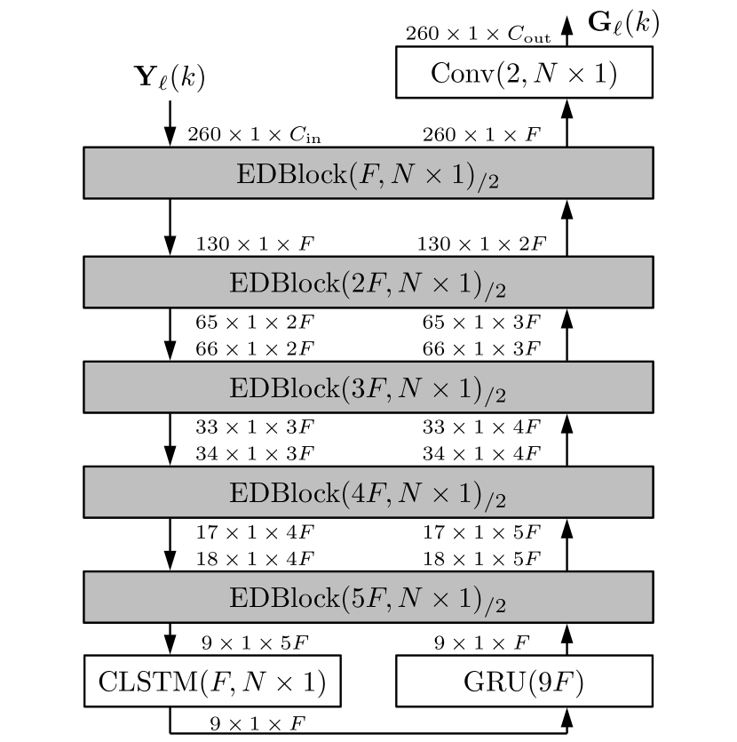
Figure 3: The EffCRN23/EffCRN23lite topology using the EDBlock detailed in Fig. 1. Mismatching dimensions are matched by zero-padding (encoder) or removal (decoder).

3.2 Network Training

The models are trained using backpropagation-through-time with a sequence (utterance) length of $|\mathcal{L}_{u}|=100$ frames, corresponding to $1.6$ seconds, and a minibatch size of $|\mathcal{B}|=16$. We use the Adam optimizer with standard parameter settings as given in [27]. The learning rate is set to $10^{-4}$, which is dynamically reduced by a factor of $0.6$ upon $4$ consecutive epochs without improved validation loss. Training is stopped after the learning rate falls below $10^{-6}$, or after $10$ consecutive epochs without improved validation loss, or upon completing $70$ epochs. We train using a fixed seed that we do not optimize for. Training is performed on a single Nvidia GTX 1080 Ti. As optimization target we use the state of the art loss function by Braun and Tashev [28]

$$J =\frac{1}{|\mathcal{B}|}\sum_{u\in\mathcal{B}}\frac{1}{|\mathcal{L}_{u}|}\sum_{\ell\in\mathcal{L}_{u}}\big{(}\frac{1\!-\!\alpha}{|\mathcal{K}|}\sum_{k\in\mathcal{K}}\big{|}|\hat{S}_{\ell}(k)|^{c}-|{S}_{\ell}(k)|^{c}\big{|}^{2}$$

$$+\frac{\alpha}{|\mathcal{K}|}\sum_{k\in\mathcal{K}}\big{|}|\hat{S}_{\ell}(k)|^{c}e^{j\varphi_{{\hat{\mathrm{s}},\ell}}(k)}-|{S}_{\ell}(k)|^{c}e^{j\varphi_{\mathrm{s},\ell}(k)}\big{|}^{2}\big{)},$$ (2)

with a compression factor $c=0.3$ and $\alpha=0.3$ being a weighting between complex and magnitude contribution. The set of utterance indices per minibatch is denoted as $\mathcal{B}$, while $\mathcal{L}_{u}$ denotes the set of frame indices in utterance $u$. The phase of the enhanced and clean signal are denoted as $\varphi_{{\hat{\mathrm{s}},\ell}}(k)$ and $\varphi_{{\mathrm{s}},\ell}(k)$, respectively.

3.3 Metrics, Results, and Discussion

For the instrumental evaluation we use perceptual evaluation of speech quality (PESQ) [29], $\Delta\mathrm{SNR}=\mathrm{SNR}_{\mathrm{out}}-\mathrm{SNR}_{\mathrm{in}}$ and DNSMOS [30]. Signal levels for SNR calculation are determined following ITU-P.56 [26]. Parameter count and #FLOPs/frame are reported based on our implementation in Tensorflow 2.7 [31]. The evaluation results are averaged over all unseen noise types and all SNRs of the test set and presented in Table 1.

The baseline FCRN [6] shows the best performance in all metrics although at a high computational complexity of $1.5$ GFLOPs/frame. The efficient CRUSE networks computationally operate at a significantly lower #FLOPs/frame, but in our setup require even more parameters than the FCRN. The FCRN15 scores close to the baseline in all reported measures, being just $0.06$ PESQ points and $0.19$ dB in $\Delta$SNR below, but with only $16.8\%$ of parameters and $8.2\%$ of computational complexity. The EffCRN23 has a slightly higher number of parameters but still stays below $1$ M and reduces computational complexity even further: With $41$ MFLOPs/frame the EffCRN23 requires only $3\%$ of computational complexity of the original FCRN at the price of $0.11$ PESQ points and $0.38$ dB $\Delta$SNR. Downscaling the architecture to the EffCRN23lite reduces computational complexity to $1.1\%$ with still moderate losses in PESQ (0.15) and $\Delta$SNR ($0.31$ dB). DNSMOS results are close, with the EffCRN23 being the best among the efficient models.

Figs. 4 and 5 show an overview of all models' performance in terms of $\Delta$SNR ($\circ$) and PESQ ($\ast$) over #FLOPS/frame and parameter count while the respective DNSMOS values can be seen in Table 1. In the efficient network regime, the FCRN15 excels over the CRUSE5 in all reported metrics PESQ, DNSMOS, $\Delta$SNR, with lower parameter count (-98%) and #FLOPS/frame (-32%). In the highly efficient network regime, the EffCRN23lite excels over the CRUSE4 in all reported metrics (-94% parameters and -20% #FLOPS/frame), showing that our FCRN/EffCRN family of networks provides best-in-class network topologies for speech enhancement.

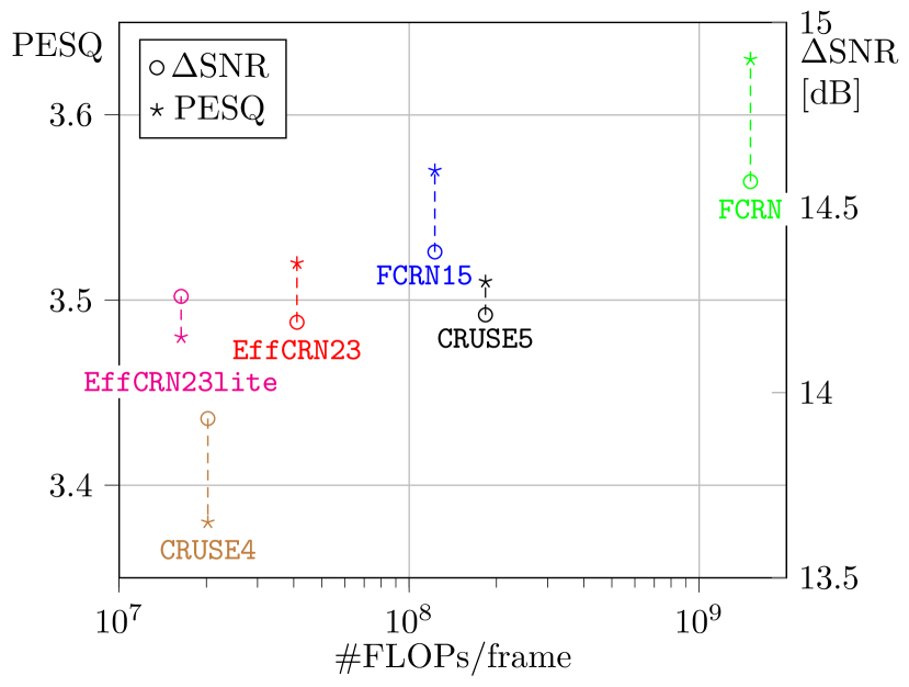
Figure 4: PESQ and $\Delta$SNR over #FLOPs/frame. The EffCRN23lite model excels over the CRUSE baselines in PESQ, $\Delta$SNR, and FLOPs/frame. Data from Table 1.

Table 1: Instrumental evaluation on the test set $\mathcal{D}_{\mathrm{test}}$. Best efficient network results are bold, second best underlined. Ablations in bottom part out of competition.

Method	#par.	#FLOPs/	PESQ	DNS	$\Delta\mathrm{SNR}$
		frame		MOS	[dB]
Noisy	-	-	2.30	-	-
FCRN [6]	5.2 M	1500 M	3.63	3.16	14.57
FCRN15	875 K	123 M	3.57	3.12	14.38
EffCRN23	997 K	41 M	3.52	3.13	14.19
EffCRN23lite	396 K	16 M	3.48	3.09	14.26
CRUSE5 [2]	85 M	183 M	3.53	3.11	14.20
CRUSE4 [2]	7.2 M	20 M	3.38	3.03	14.06
FCRN15$\raisebox{0.0pt}{\scriptsize{-}}\raisebox{-0.5pt}{\scriptsizeC}⃝$	777 K	112 M	3.54	3.12	14.30
FCRN15$\raisebox{0.0pt}{\scriptsize{-}}\raisebox{-0.5pt}{\scriptsizeC}⃝\raisebox{0.0pt}{\scriptsize{+}}\raisebox{-0.5pt}{\scriptsizeG}⃝$	7.4 M	125 M	3.51	3.13	14.17
FCRN15$\raisebox{0.0pt}{\scriptsize{+}}\raisebox{-0.5pt}{\scriptsizeF}⃝$	209 K	29 M	3.41	3.05	14.14
FCRN15$\raisebox{0.0pt}{\scriptsize{+}}\raisebox{-0.5pt}{\scriptsizeF}⃝\raisebox{0.0pt}{\scriptsize{+}}\raisebox{-0.5pt}{\scriptsizeD}⃝\raisebox{0.0pt}{\scriptsize{+}}\raisebox{-0.5pt}{\scriptsizeP}⃝$	665 K	41 M	3.44	3.04	14.07

Furthermore, Table 1 (lower half) and Table 2 show the impact of our intermediate steps (-\raisebox{-0.5pt}{\scriptsizeC}⃝,+\raisebox{-0.5pt}{\scriptsizeG}⃝,+\raisebox{-0.5pt}{\scriptsizeD}⃝,+\raisebox{-0.5pt}{\scriptsizeP}⃝,+\raisebox{-0.5pt}{\scriptsizeF}⃝) on computational complexity and model performance. Experimenting with the recurrent layers of the FCRN15 shows a slight loss of performance in case of both removal of the second CLSTM (FCRN15-\raisebox{-0.5pt}{\scriptsizeC}⃝) and its replacement with a GRU (FCRN15-\raisebox{-0.5pt}{\scriptsizeC}⃝+\raisebox{-0.5pt}{\scriptsizeG}⃝). With $7.2$ M parameters, however, the latter is simply too large. As visible in Table 2, just increasing network depth alone (FCRN15+\raisebox{-0.5pt}{\scriptsizeD}⃝) does not reduce, but increase both #parameters and #FLOPs/frame, as expected. Also shifting padding from input data towards internal data representations of the network (FCRN15+\raisebox{-0.5pt}{\scriptsizeD}⃝+\raisebox{-0.5pt}{\scriptsizeP}⃝), #FLOPs/frame can be reduced by $9$ M, yet the network remains unacceptably large ($2.8$ M). Beginning our modifications with just decreasing filter numbers and kernel sizes, leads to a very small and efficient network (FCRN15$\raisebox{0.0pt}{\scriptsize{+}}\raisebox{-0.5pt}{\scriptsizeF}⃝$), however, coming with a dramatic performance loss across all measures compared to the FCRN15, see Table 1 again. This motivates in a first step to combine the deep network with smaller and fewer filter kernels (FCRN15+\raisebox{-0.5pt}{\scriptsizeF}⃝+\raisebox{-0.5pt}{\scriptsizeD}⃝+\raisebox{-0.5pt}{\scriptsizeP}⃝), which yields a still small ($665$ K) and efficient ($41$ MFLOPS/frame) network. To regain performance in a second step, we revisit the initial idea of modifying recurrent processing by replacing the FCRN15+\raisebox{-0.5pt}{\scriptsizeF}⃝+\raisebox{-0.5pt}{\scriptsizeD}⃝+\raisebox{-0.5pt}{\scriptsizeP}⃝'s second CLSTM with a GRU (FCRN15+\raisebox{-0.5pt}{\scriptsizeF}⃝+\raisebox{-0.5pt}{\scriptsizeD}⃝+\raisebox{-0.5pt}{\scriptsizeP}⃝-\raisebox{-0.5pt}{\scriptsizeC}⃝+\raisebox{-0.5pt}{\scriptsizeG}⃝) which is in total then identical to the EffCRN23. Due to the small bottleneck feature representation, this network manages to regain $0.08$ PESQ-points and $0.09$ DNSMOS-points while maintaining very low complexity and staying below $1$ M parameters.

4 Conclusions

In this paper, we have introduced the FCRN15 topology and newly proposed the EffCRN23 class of networks for speech enhancement. Significant reductions in model parameter count as well as #FLOPs/frame compared to the FCRN baseline can be achieved by smaller kernels and an only linear increase (decrease) of the number of filters in the encoder (decoder). This allows then to increase the network depth, but requires learnable skip connections and re-introduction of a non-convolutional (GRU) layer in the sparse bottleneck. The efficient models retain high performance with the EffCRN23lite requiring $7.6\%$ of parameters and $1.1\%$ of FLOPs/frame compared to the baseline topology. We furthermore show that the FCRN15 and EffCRN23lite outperform the CRUSE5 and CRUSE4 networks, respectively, w.r.t. PESQ and DNSMOS and $\Delta$SNR, while requiring about 94% less parameters and about 20% less #FLOPs/frame.

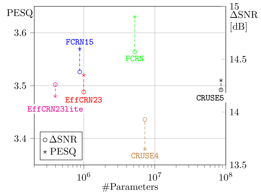
Figure 5: PESQ and $\Delta$SNR over #parameters. The EffCRN23lite model excels over the CRUSE baselines w.r.t PESQ, $\Delta$SNR, and #parameters. Data from Table 1.

Table 2: Computational impact of topology modifications.

Method	#par.	#FLOPs/frame
FCRN15	875 K	123 M
FCRN15-\raisebox{-0.5pt}{\scriptsizeC}⃝	777 K	112 M
FCRN15-\raisebox{-0.5pt}{\scriptsizeC}⃝+\raisebox{-0.5pt}{\scriptsizeG}⃝	7400 K	125 M
FCRN15+\raisebox{-0.5pt}{\scriptsizeD}⃝	2800 K	183 M
FCRN15+\raisebox{-0.5pt}{\scriptsizeD}⃝+\raisebox{-0.5pt}{\scriptsizeP}⃝	2800 K	172 M
FCRN15+\raisebox{-0.5pt}{\scriptsizeF}⃝	209 K	29 M
FCRN15+\raisebox{-0.5pt}{\scriptsizeF}⃝+\raisebox{-0.5pt}{\scriptsizeD}⃝+\raisebox{-0.5pt}{\scriptsizeP}⃝	665 K	41 M

References

- [1] I. Fedorov, M. Stamenovic, C. Jensen, L.-C. Yang, A. Mandell, Y. Gan, M. Mattina, and P. N. Whatmough, ``TinyLSTMs: Efficient Neural Speech Enhancement for Hearing Aids,'' in Proc. of Interspeech, Shanghai, China, Oct. 2020, pp. 4054–4058.
- [2] S. Braun, H. Gamper, C. K. A. Reddy, and I. Tashev, ``Towards Efficient Models for Real-Time Deep Noise Suppression,'' in Proc. of ICASSP, Toronto, ON, Canada, Jun. 2021, pp. 656–660.
- [3] K. Tan and D. Wang, ``Compressing Deep Neural Networks for Efficient Speech Enhancement,'' in Proc. of ICASSP, Toronto, Canada, Jun. 2021, pp. 8358–8362.
- [4] J.-M. Valin, ``A Hybrid DSP/Deep Learning Approach to Real-Time Full-Band Speech Enhancement,'' in Proc. of MMSP, Vancouver, BC, Canada, Aug. 2018, pp. 43–47.
- [5] D. Wang and J. Chen, ``Supervised Speech Separation Based on Deep Learning: An Overview,'' IEEE/ACM Transactions on Audio, Speech, and Language Processing, vol. 26, no. 10, pp. 1702–1726, Oct. 2018.
- [6] M. Strake, B. Defraene, K. Fluyt, W. Tirry, and T. Fingscheidt, ``INTERSPEECH 2020 Deep Noise Suppression Challenge: A Fully Convolutional Recurrent Network (FCRN) for Joint Dereverberation and Denoising,'' in Proc. of Interspeech, Shanghai, China, Oct. 2020, pp. 2467–2471.
- [7] D. S. Williamson, Y. Wang, and D. L. Wang, ``Complex Ratio Masking for Monaural Speech Separation,'' IEEE/ACM Transactions on Audio, Speech, and Language Processing, vol. 24, no. 3, pp. 483–492, Mar. 2016.
- [8] Y. Hu, Y. Liu, S. Lv, M. Xing, S. Zhang, Y. Fu, J. Wu, B. Zhang, and L. Xie, ``DCCRN: Deep Complex Convolution Recurrent Network for Phase-Aware Speech Enhancement,'' in Proc. of Interspeech, Shanghai, China, Oct. 2020, pp. 2472––2476.
- [9] S. R. Park and J. W. Lee, ``A Fully Convolutional Neural Network for Speech Enhancement,'' in Proc. of Interspeech, Stockholm, Sweden, Aug. 2017, pp. 1993––1997.
- [10] M. Strake, B. Defraene, K. Fluyt, W. Tirry, and T. Fingscheidt, ``Fully Convolutional Recurrent Networks for Speech Enhancement,'' in Proc. of ICASSP, Barcelona, Spain, May 2020, pp. 6674–6678.
- [11] Z. Xu, S. Elshamy, Z. Zhao, and T. Fingscheidt, ``Components Loss for Neural Networks in Mask-Based Speech Enhancement,'' EURASIP Journal on Audio, Speech, and Music Processing, vol. 2021, no. 1, pp. 1–20, Jul. 2021.
- [12] F. Weninger, H. Erdogan, S. Watanabe, E. Vincent, J. L. Roux, J. R. Hershey, and B. Schuller, ``Speech Enhancement with LSTM Recurrent Neural Networks and its Application to Noise-Robust ASR,'' in Proc. of LVA/ICA, Liberec, Czech Republic, Aug. 2015, pp. 91–99.
- [13] S. Hochreiter and J. Schmidhuber, ``Long Short-Term Memory,'' Neural Computation, vol. 9, no. 8, pp. 1735–1780, Nov. 1997.
- [14] K. Cho, B. van Merriënboer, D. Bahdanau, and Y. Bengio, ``On the Properties of Neural Machine Translation: Encoder-Decoder Approaches,'' in Proc. of SSST, Doha, Qatar, Oct. 2014, pp. 103–111.
- [15] K. Tan and D. Wang, ``Convolutional Recurrent Neural Network for Real-Time Speech Enhancement,'' in Proc. of Interspeech, Hyderabad, India, Sep. 2018, pp. 3229–3233.
- [16] H. Zhao, S. Zarar, I. Tashev, and C.-H. Lee, ``Convolutional-Recurrent Neural Networks for Speech Enhancement,'' in Proc. of ICASSP, Calgary, AB, Canada, Apr. 2018, pp. 2401–2405.
- [17] H. Schröter, T. Rosenkranz, A.-N. Escalante-B, and A. Maier, ``Low Latency Speech Enhancement for Hearing Aids Using Deep Filtering,'' IEEE/ACM Transactions on Audio, Speech, and Language Processing, vol. 30, pp. 2716 – 2728, Aug. 2022.
- [18] M. Tan and Q. Le, ``EfficientNet: Rethinking Model Scaling for Convolutional Neural Networks,'' in Proc. of ICML, Long Beach, CA, USA, Jun. 2019, pp. 6105–6114.
- [19] M. Strake, B. Defraene, K. Fluyt, W. Tirry, and T. Fingscheidt, ``Speech Enhancement by LSTM-Based Noise Suppression Followed by CNN-Based Speech Restoration,'' EURASIP Journal on Advances in Signal Processing, vol. 2020, no. 49, pp. 1–26, Dec. 2020.
- [20] A. L. Maas, A. Y. Hannun, and A. Y. Ng, ``Rectifier Nonlinearities Improve Neural Network Acoustic Models,'' in Proc. of ICML, Atlanta, GA, USA, Jun. 2013.
- [21] X. Shi, Z. Chen, H. Wang, D.-Y. Yeung, W. kin Wong, and W. chun Woo, ``Convolutional LSTM Network: A Machine Learning Approach for Precipitation Nowcasting,'' in Proc. of NIPS, Montreal, QC, Canada, Dec. 2015, pp. 802–810.
- [22] J. Garofolo, D. Graff, D. Paul, and D. Pallett, ``CSR-I (WSJ0) Complete,'' Linguistic Data Consortium, Philadelphia, 2007.
- [23] J. Thiemann, N. Ito, and E. Vincent, ``The Diverse Environments Multi-Channel Acoustic Noise Database: A Database of Multichannel Environmental Noise Recordings,'' J. Acoust. Soc. Am, vol. 133, no. 5, pp. 3591–3591, 2013.
- [24] D. B. Dean, S. Sridharan, R. J. Vogt, and M. W. Mason, ``The QUT-NOISE-TIMIT Corpus for the Evaluation of Voice Activity Detection Algorithms,'' in Proc. of Interspeech, Makuhari, Japan, Sep. 2010, pp. 3110–3113.
- [25] Speech Processing, Transmission and Quality Aspects (STQ); Speech Quality Performance in the Presence of Background Noise; Part 1: Background Noise Simulation Technique and Background Noise Database, ETSI EG 202 396-1, Sep. 2008.
- [26] ITU, Rec. P.56: Objective Measurement of Active Speech Level, International Telecommunication Union, Telecommunication Standardization Sector (ITU-T), Dec. 2011.
- [27] D. P. Kingma and J. Ba, ``Adam: A Method for Stochastic Optimization,'' in Proc. of ICLR, San Diego, CA, USA, May 2015, pp. 1–15.
- [28] S. Braun and I. Tashev, ``A Consolidated View of Loss Functions for Supervised Deep Learning-Based Speech Enhancement,'' in Proc. of TSP, Brno, Czech Republic, Jul. 2021, pp. 72–76.
- [29] ITU-T, Rec. P.862.2: Wideband Extension to Recommendation P862 for the Assesment of Wideband Telephone Networks and Speech Codecs, International Telecommunication Union, Telecommunication Standardization Sector (ITU-T), Feb. 2001.
- [30] C. K. A. Reddy, V. Gopal, and R. Cutler, ``DNSMOS: A Non-Intrusive Perceptual Objective Speech Quality Metric to Evaluate Noise Suppressors,'' in Proc. of ICASSP, Toronto, ON, Canada, Jun. 2021, pp. 6493–6497.
- [31] M. Abadi, P. Barham, J. Chen, Z. Chen, A. Davis, J. Dean, M. Devin, S. Ghemawat, G. Irving, M. Isard et al., ``TensorFlow: A System for Large-Scale Machine Learning,'' in Proc. of OSDI, 2016, pp. 265–283.