Conformal Prediction with Missing Values

Abstract

Conformal prediction is a theoretically grounded framework for constructing predictive intervals. We study conformal prediction with missing values in the covariates – a setting that brings new challenges to uncertainty quantification. We first show that the marginal coverage guarantee of conformal prediction holds on imputed data for any missingness distribution and almost all imputation functions. However, we emphasize that the average coverage varies depending on the pattern of missing values: conformal methods tend to construct prediction intervals that under-cover the response conditionally to some missing patterns. This motivates our novel generalized conformalized quantile regression framework, missing data augmentation, which yields prediction intervals that are valid conditionally to the patterns of missing values, despite their exponential number. We then show that a universally consistent quantile regression algorithm trained on the imputed data is Bayes optimal for the pinball risk, thus achieving valid coverage conditionally to any given data point. Moreover, we examine the case of a linear model, which demonstrates the importance of our proposal in overcoming the heteroskedasticity induced by missing values. Using synthetic and data from critical care, we corroborate our theory and report improved performance of our methods.

1 Introduction

By leveraging increasingly large data sets, statistical algorithms and machine learning methods can be used to support high-stakes decision-making problems such as autonomous driving, medical or civic applications, and more. To ensure the safe deployment of predictive models it is crucial to quantify the uncertainty of the resulting predictions, communicating the limits of predictive performance. Uncertainty quantification attracts a lot of attention in recent years, particularly methods that are based on Conformal Prediction (CP) (Vovk et al.,, 2005; Papadopoulos et al.,, 2002; Lei et al.,, 2018). CP provides controlled predictive regions for any underlying predictive algorithm (e.g., neural networks and random forests), in finite samples with no assumption on the data distribution except for the exchangeability of the train and test data. More precisely, for a miscoverage rate $\alpha\in[0,1]$, CP outputs a marginally valid prediction interval $\widehat{C}_{\alpha}$ for the test response $Y$ given its corresponding covariates $X$, that is:

$$\mathds{P}(Y\in\widehat{C}_{\alpha}(X))\geq 1-\alpha.$$ (1)

Split CP (Papadopoulos et al.,, 2002; Lei et al.,, 2018) achieves Eq. (1) by keeping a hold-out set, the calibration set, used to evaluate the performance of a fixed predictive model.

At the same time, as the volume of data increases, the volume of missing values also increases. There is a vast literature on this topic (Little,, 2019; Josse and Reiter,, 2018), and a recent survey even identified more than 150 different implementations (Mayer et al.,, 2019). Missing values create additional challenges to the task of supervised learning, as traditional machine learning algorithms can not handle incomplete data (Josse et al.,, 2019; Le Morvan et al., 2020b, ; Le Morvan et al., 2020a, ; Le Morvan et al.,, 2021; Ayme et al.,, 2022; Van Ness et al.,, 2022). One of the most popular strategies to deal with missing values suggests imputing the missing entries with plausible values to get completed data, on which any analysis can be performed. The drawback of this “impute-then-predict” approach is that single imputation can distort the joint and marginal distribution of the data. Yet, Josse et al., (2019); Le Morvan et al., 2020b ; Le Morvan et al., (2021) showed that such impute-then-predict strategies are Bayes consistent, under the assumption that a universally consistent learner is applied on an imputed data set. However, this line of work focuses on point prediction with missing values that aim to predict the most likely outcome. In contrast, our goal is quantifying predictive uncertainty, which was not explored with missing values although its enormous importance.

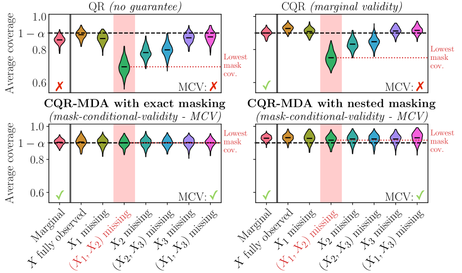
(a) Coverage of the predictive intervals depending on which features are missing, among the 3 features. Evaluation over 200 runs.

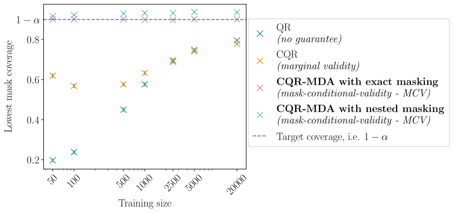
(b) Lowest mask coverage as a function of the training size. Results evaluated over 100 repetitions, and the (tiny) error bars correspond to standard errors.

Figure 1: Methods are Quantile Regression (QR), Conformalized Quantile Regression (CQR), and two novel procedures CP-MDA-Exact and CP-MDA-Nested, on top of CQR. Settings are given in Section 7, in a nutshell: data follows a Gaussian linear model where missing values are independent of everything else and of proportion 20%; the dimension of the problem is 3 in Figure 1(a) while in 1(b) it is 10.

Contributions.

We study CP with missing covariates. Specifically, we study downstream quantile regression (QR) based CP, like CQR (Romano et al.,, 2019), on impute-then-predict strategies. Still, the proposed approaches also encapsulate other regression basemodels, and even classification.

After setting background in Section 2, our first contribution is showing that CP on impute-then-predict is marginally valid regardless of the model, missingness distribution, and imputation function (Section 3).

Then, we focus on the specificity of uncertainty quantification with missing values. In Section 4, we describe how different masks (i.e. the set of observed features) introduce additional heteroskedasticity: the uncertainty on the output strongly depends on the set of predictive features observed. We therefore focus on achieving valid coverage conditionally on the mask, coined MCV – Mask-Conditional-Validity. MCV is desirable in practice, as occurrence of missing values are linked to important attributes (see Section 5).

Traditional approaches such as QR and CQR fail to achieve MCV because they do not account for this core connection between missing values and uncertainty. This is illustrated on synthetic data in Figure 1. In Figure 1(a), a toy example with only 3 features, thus $2^{3}-1=7$ possible masks, shows how the coverage of QR and CQR varies depending on the mask. Both methods dramatically undercover when the most important variable ($X_{2}$) is missing, and the loss of coverage worsens when additional features are missing. In particular, for each method, one mask ($X_{1}$ and $X_{2}$ missing, highlighted in red) leads to the lowest mask coverage. Achieving MCV corresponds to a lowest mask coverage greater than $1-\alpha$. In Figure 1(b), the dimension is 10: instead of the $2^{10}-1=1023$ different masks, we only report the lowest mask coverage for increasing sample sizes. It highlights that QR (green $\times$) and CQR (orange $\times$) do not meet the lowest mask coverage target of 90%, even for large sample sizes.

This motivates our second contribution: we show in Section 5 how to form prediction intervals that are MCV. This is highly challenging since there are exponentially many possible patterns to consider. Therefore, the naive solution to perform a calibration for each mask would fail as in finite samples, we often observe test samples with a mask that have low (or even null) frequency of appearance in the calibration set. To tackle this issue, we suggest two conformal methods that share the same core idea of missing data augmentation (MDA): the calibration data is artificially masked to match the mask of the point we consider at test time. The first method, CP-MDA with exact masking, relies on building an ideal calibration set for which the data points have the exact same mask as of the test point. We show its MCV under exchangeability and Missing Completely At Random assumptions. Our second method, CP-MDA with nested masking, does not require such an ideal calibration set. Instead, we artificially construct a calibration set in which the data points have at least the same mask as the test point, i.e., this artificial masking results in calibration points having possibly more missing values than the test point. We show the latter method also achieves the desired coverage conditional on the mask, but at the cost of an additional assumption for validity: stochastic domination of the quantiles. Figure 1 illustrates those findings: both methods are MCV, as their lowest mask coverage is above $1-\alpha$.

Our third contribution further supports our design choice to use QR. We show that QR on impute-then-predict strategy is Bayes-consistent – it can achieve the strongest form of coverage conditional on the observed test features (Section 6).

Lastly, we support our proposal using both (semi)-synthetic experiments and real medical data (Section 7). The code to reproduce our experiments is available on GitHub.

2 Background

Background on missing values. Consider a data set with $n$ exchangeable realizations of the random variable $(X,M,Y)\in\mathds{R}^{d}\times\{0,1\}^{d}\times\mathds{R}$: $\left\{\left(X^{(k)},M^{(k)},Y^{(k)}\right)\right\}_{k=1}^{n}$, where $X$ represents the features, $M$ the missing pattern, or mask, and $Y$ an outcome to predict. For $j\in\llbracket 1,d\rrbracket$, $M_{j}=0$ when $X_{j}$ is observed and $M_{j}=1$ when $X_{j}$ is missing, i.e. NA (Not Available). We note $\mathcal{M}=\{0,1\}^{d}$ the set of masks. For a pattern $m\in\mathcal{M},X_{\text{obs}(m)}$ is the random vector of observed components, and $X_{\text{mis}(m)}$ is the random vector of unobserved ones. For example, if we observe $(\texttt{NA},6,2)$ then $m=(1,0,0)$ and $X_{\text{obs}(m)}=(6,2)$. Our goal is to predict a new outcome $Y^{(n+1)}$ given $X_{\text{obs}(M^{(n+1)})}^{(n+1)}$ and $M^{(n+1)}$.

Assumption A1 (exchangeability).

The random variables $\left(X^{(k)},M^{(k)},Y^{(k)}\right)_{k=1}^{n+1}$ are exchangeable.

Following Rubin, (1976), we consider three well-known missingness mechanisms.

Definition 2.1 (Missing Completely At Random (MCAR)).

For any $m\in\mathcal{M}$, $\mathds{P}\left(M=m|X\right)=\mathds{P}\left(M=m\right)$.

Definition 2.2 (Missing At Random (MAR)).

For any $m\in\mathcal{M}$, $\mathds{P}\left(M=m|X\right)=\mathds{P}\left(M=m|X_{\text{obs}(m)}\right)$.

Definition 2.3 (Missing Non At Random (MNAR)).

If the missing data is not MAR, it is MNAR. Thus, its probability distribution depends on $X$, including the missing values.

Impute-then-predict. As most predictive algorithms can not directly handle missing values, we impute the incomplete data using an imputation function $\Phi$ which maps observed values to themselves and missing values to a function of the observed values. With notations from Le Morvan et al., (2021) we note $\phi^{m}:\mathds{R}^{|\rm{obs}(m)|}\rightarrow\mathds{R}^{|\mathrm{mis}(m)|}$ the imputation function which takes as input observed values and outputs imputed values, i.e. plausible values, given a mask $m\in\mathcal{M}$. Then, the imputation function $\Phi$ belongs to $\begin{aligned} \mathcal{F}^{I}:=&\left\{\right.\Phi:\mathds{R}^{d}\times\mathcal{M}\rightarrow\mathds{R}^{d}:\forall j\in\llbracket 1,d\rrbracket,\\ &\left.\Phi_{j}\left(X,M\right)=X_{j}\mathds{1}_{M_{j}=0}+\phi_{j}^{M}\left(X_{\text{obs}(M)}\right)\mathds{1}_{M_{j}=1}\right\}.\end{aligned}$ Additionally, $\mathcal{F}^{I}_{\infty}$ is the restriction of $\mathcal{F}^{I}$ to $\mathcal{C}^{\infty}$ functions which include deterministic imputation, such as mean imputation or imputation by regression. The imputed data set is formed by the realizations of the $n$ random variables $\left(\Phi\left(X,M\right),M,Y\right)$. In practice, $\Phi$ is obtained as the result of an algorithm $\mathcal{I}$ trained on $\left\{\left(X^{(k)},M^{(k)}\right)\right\}_{k=1}^{n+1}$.

Assumption A2 (Symmetrical imputation).

The imputation function $\Phi$ is the output of an algorithm $\mathcal{I}$ treating its input data points symmetrically: $\mathcal{I}((X^{(\sigma(k))},M^{(\sigma(k))})_{k=1}^{n+1})\overset{(d)}{=}\mathcal{I}((X^{(k)},M^{(k)})_{k=1}^{n+1})$ conditionally on $(X^{(k)},M^{(k)})_{k=1}^{n+1}$ and for any permutation $\sigma$ on $\llbracket 1,n+1\rrbracket$.

Assumption A2 is very mild and satisfied by all existing imputation methods for exchangeable data. In particular, it is valid for iterative regression imputation which allows out-of-sample imputation.

Background on (split) conformal prediction. Split, or inductive, CP (SCP) (Papadopoulos et al.,, 2002; Lei et al.,, 2018) builds predictive regions by first splitting the $n$ points of the training set into two disjoint sets $\rm{Tr},\rm{Cal}\subset\llbracket 1,n\rrbracket$, to create a proper training set, $\rm{Tr}$, and a calibration set, $\rm{Cal}$. On the proper training set, a model $\hat{f}$ (chosen by the user) is fitted, and then used to predict on the calibration set. Conformity scores $S_{\rm{Cal}}=\{(s(X^{(k)},Y^{(k)}))_{k\in\rm{Cal}}\}$ are computed to assess how well the fitted model $\hat{f}$ predicts the response values of the calibration points. For example, Conformalized Quantile Regression (CQR, Romano et al.,, 2019) fits two quantile regressions $\hat{q}_{\text{low}}$ and $\hat{q}_{\text{upp}}$, on the proper training set. The conformity scores are defined by $s(x,y)=\max(\hat{q}_{\text{low}}(x)-y,y-\hat{q}_{\text{upp}}(x))$. Finally, a corrected $(1-\tilde{\alpha})$-th quantile of these scores $\widehat{Q}_{1-\tilde{\alpha}}(S_{\rm{Cal}})$ is computed (called correction term) to define the predictive region: $\widehat{C}_{\alpha}(x):=\{y\text{ such that }s(y,\hat{f}(x))\leq\widehat{Q}_{1-\tilde{\alpha}}(S_{\rm{Cal}})\}$. An illustration of CQR is provided in Appendix B.

This procedure satisfies Eq. (1) for any $\hat{f}$, any (finite) sample size $n$, as long as the data points are exchangeable. Moreover, if the scores are almost surely distinct, the coverage holds almost exactly: $\mathds{P}(Y\in\widehat{C}_{\alpha}(X))\leq 1-\alpha+\frac{1}{\#\rm{Cal}+1}$.

For more details on SCP, we refer to Angelopoulos and Bates, (2023); Vovk et al., (2005), as well as to Manokhin, (2022).

3 Warm-up: marginal coverage with NAs

A first idea to get valid predictive intervals $\widehat{C}_{\alpha}(X,M)$ in the presence of missing values $M$ is to apply CP in combination with impute-then-predict, which we refer to as impute-then-predict+conformalization. More details on this approach are given in Section C.1 for both classification and regression tasks, although our main focus is regression. It turns out that such a simple approach is marginally (exactly) valid.

Definition 3.1 (Marginal validity).

A method outputting intervals $\widehat{C}_{\alpha}$ is marginally valid if the following lower bound is satisfied, and exactly valid if the following upper bound is also satisfied:

$$1-\alpha\underset{\text{validity}}{\leq}\mathds{P}\left(Y^{(n+1)}\in\widehat{C}_{\alpha}\left(X^{(n+1)},M^{(n+1)}\right)\right)$$

$$\underset{\text{exact validity}}{\leq}1-\alpha+\frac{1}{\#\rm{Cal}+1}.$$

Indeed, symmetric imputation preserves exchangeability.

Lemma 3.2 (Imputation preserves exchangeability).

Let A1 hold. Then, for any missing mechanism, for any imputation function $\Phi$ satisfying A2, the imputed random variables $\left(\Phi\left(X^{(k)},M^{(k)}\right),M^{(k)},Y^{(k)}\right)_{k=1}^{n+1}$ are exchangeable.

Note that if we replace A1 by an i.i.d. assumption, the imputed data set is only exchangeable but not i.i.d. without further assumptions on $\mathcal{I}$. Indeed, even simple mean imputation breaks independence.

Proposition 3.3 ((Exact) validity of impute-then-predict+conformalization).

If A1 and A2 are satisfied, impute-then-predict+conformalization is marginally valid. If moreover the scores are almost surely distinct, it is exactly valid.

This is an important first positive result (proved in Section C.2) showing that CP applied on an imputed data set has the same validity properties as on complete data, regardless of the missing value mechanism (MCAR, MAR or MNAR) and of the symmetric imputation scheme. Note that similar propositions could be derived for full CP (Vovk et al.,, 2005) and Jackknife+ (Barber et al., 2021b, ).

Proposition 3.3 complements the work by Yang, (2015), that also guarantees marginal coverage for full CP, with the striking difference of having a complete training data.

4 Challenge: NAs induce heteroskedasticity

To better understand the interplay between missing values and conditional coverage with respect to the mask, we consider an illustrative example of a Gaussian linear model.

Model 4.1 (Gaussian linear model).

The data is generated according to a linear model and the covariates are Gaussian conditionally to the pattern:

• $Y=\beta^{T}X+\varepsilon$, $\varepsilon\sim\mathcal{N}(0,\sigma^{2}_{\varepsilon})\perp\!\!\!\!\perp(X,M)$, $\beta\in\mathds{R}^{d}$.

• for all $m\in\mathcal{M}$, there exist $\mu^{m}$ and $\Sigma^{m}$ such that $X|(M=m)\sim\mathcal{N}(\mu^{m},\Sigma^{m}).$

In particular, 4.1 is verified when $X$ is Gaussian and the missing data is MCAR. 4.1 is more general: it even includes MNAR examples (Ayme et al.,, 2022).

Proposition 4.2 (Oracle intervals).

The oracle predictive interval is defined as the smallest valid interval knowing $X_{\rm{obs}(M)}$ and $M$. Under 4.1, its length only depends on the mask. For any $m\in\mathcal{M}$ this oracle length is:

$$\mathcal{L}^{*}_{\alpha}(m)=2q^{\mathcal{N}(0,1)}_{1-\frac{\alpha}{2}}\sqrt{\beta^{T}_{\mathrm{mis}(m)}\Sigma^{m}_{\mathrm{mis}|\rm{obs}}\beta_{\mathrm{mis}(m)}+\sigma^{2}_{\varepsilon}}.$$ (2)

See Appendix D for the definition of $\mu^{m}_{\mathrm{mis}|\rm{obs}}$ and $\Sigma^{m}_{\mathrm{mis}|\rm{obs}}$ and the quantiles of $Y|(X_{\rm{obs}(m)},M=m)$.

Eq. (2) stresses that even when the noise of the generative model is homoskedastic, missing values induce heteroskedasticity. Indeed, the covariance of the conditional distribution of $Y|(X_{\rm{obs}(m)},M=m)$ depends on $m$. Furthermore, the uncertainty increases when missing values are associated with larger regression coefficients (i.e. the most predictive variables): if $\beta_{\mathrm{mis}(m)}$ is large, then $\mathcal{L}^{*}_{\alpha}(m)$ is also large, as $\Sigma^{m}_{\mathrm{mis}|\rm{obs}}$ is positive. In the extreme case where all the variables are missing, i.e. $m=(1,\cdots,1)$, $\mathcal{L}^{*}_{\alpha}(m)=2q^{\mathcal{N}(0,1)}_{1-\frac{\alpha}{2}}\sqrt{\beta\Sigma^{m}\beta^{T}+\sigma_{\varepsilon}^{2}}=q^{Y}_{1-\frac{\alpha}{2}}-q^{Y}_{\frac{\alpha}{2}}$. On the contrary, if $m=(0,\cdots,0)$ (that is all $X_{j}$ are observed), $\beta_{\mathrm{mis}(m)}$ is empty and $\mathcal{L}^{*}_{\alpha}(m)=2q^{\mathcal{N}(0,1)}_{1-\frac{\alpha}{2}}\sigma_{\varepsilon}=q^{\varepsilon}_{1-\frac{\alpha}{2}}-q^{\varepsilon}_{\frac{\alpha}{2}}$. We illustrate this induced heteroskedasticity and the impact of the predictive power in Figure 1(a), and in Appendix D along with a discussion emphasizing that even with the Bayes predictor for the conditional mean, mean-based CP does not yield intervals that are MCV.

The above analysis motivates the following two design choices we make in this work. First, we advocate working with QR models rather than classic regression ones, as the former can handle heteroskedastic data. Second, we recommend providing the mask information to the model in addition to the input covariates, as the mask may further encourage the model to construct an interval with a length adaptive to the given mask. Therefore, we focus on CQR (Romano et al.,, 2019), an adaptive version of SCP, and concatenate the mask to the features. However, the predictive intervals of this procedure may not necessarily provide valid coverage conditionally on the masks, especially in finite samples as shown in Figure 1(b) (orange crosses). This is because the quality of the prediction at some $(X,M)$ depends strongly on $M$, as there is an exponential number of patterns ($2^{d}$) for a finite training size, whereas the correction term is calculated independently of the masks.

5 Achieving mask-conditional-validity (MCV)

We now aim at achieving mask-conditional-validity (MCV) defined as follows using an ordering on the masks.

Definition 5.1 (Included masks).

Let $(\mathring{m},\breve{m})\in\mathcal{M}^{2}$, $\mathring{m}\subset\breve{m}$ if for any $j\in\llbracket 1,d\rrbracket$ such that $\mathring{m}_{j}=1$ then $\breve{m}_{j}=1$, i.e. $\breve{m}$ includes at least the same missing values than $\mathring{m}$.

Definition 5.2 (MCV).

A method is MCV if for any $m\in\mathcal{M}$ the followinglower bound is satisfied, and exactly MCV if for any $m\in\mathcal{M}$ the followingupper bound is also satisfied:

$$1-\alpha\!\!\!\underset{\text{valid}}{\leq}\!\!\mathds{P}\left(Y^{(n+1)}\in\widehat{C}_{\alpha}\left(X^{(n+1)},m\right)|M^{(n+1)}=m\right)$$

$$\underset{\text{exactly valid}}{\leq}1-\alpha+\frac{1}{\#\rm{Cal}^{m}+1},$$

where $\rm{Cal}^{m}=\left\{k\in\rm{Cal}\text{ such that }m^{(k)}\subset m\right\}$.

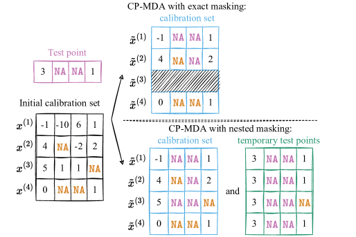
Figure 2: CP-MDA illustration. Augmented calibration set according to one test point. For CP-MDA-Nested, the augmented masks of the calibration set are also applied temporarily to the test point.

On the relevance of MCV.

In a medical application context, it is very common to have missing data completely at random (MCAR) when a measurement device fails or the medical team forgot to fill out some forms. As a general rule, from an equity standpoint, a patient whose data is missing should not be penalized (because of “bad luck”) by being assigned a prediction interval that is less likely to include the true response than if the data were complete.

Furthermore, the mask can also be linked to an external unobserved feature corresponding to a meaningful category. Consider the problem of predicting a disease among a population. Aggregating data from multiple hospitals with different practices and measurement devices can imply different features are observed for each patient. This can be viewed as a MCAR setting when identically distributed patients are assigned an hospital at random. Patterns are then linked to the cities, that themselves are related to socio-economical data.

Overall, the missing patterns form meaningful categories and ensuring MCV yields more equitable treatment. Therefore, a method achieving marginal coverage by systematically failing on a given pattern, even in a MCAR setting, is not suitable. Finally, in non-MCAR cases, the pattern may be exactly related to critical discriminating features.

5.1 Missing Data Augmentation (MDA)

To obtain a MCV procedure, we suggest modifying the calibration set according to the mask of the test point, while the training step is unchanged. More precisely, the mask of the test point is applied to the calibration set, as illustrated in Figure 2. The rationale is to mimic the missing pattern of the test point by artificially augmenting the calibration set with that mask. It ensures that the correction term is computed using data with (at least) the same missing values as the test point. We refer to this strategy as CP with Missing Data Augmentation (CP-MDA), and derive two versions of it. Algorithms 1 and 2 are written using CQR as the base conformal procedure, but they work with any conformal method as we describe in Section E.1.

Algorithm 1 – CP-MDA-Exact. CP-MDA with exact masking consists of keeping the artificially masked calibration points (l. 10) that have exactly the same missing pattern as the test point (l. 8). Then Algorithm 1 performs as impute-then-predict+conformalization: impute the calibration set (l. 13), predict on it and get the calibration scores (l. 14), compute their quantile to obtain the correction term (l. 17), and finally impute and predict the test point with the fixed fitted model by adding and subtracting the correction term (l. 18) to the initial conditional quantile estimates. Note that Algorithm 1 is described for one test point for simplicity but extends easily to many test points. The computations are then shared: the training part (l. 3-6) is common to any test point and the correction term (l. 8-17) can be reused for any new test point with the same mask.

Algorithm 1 CP-MDA-Exact (with CQR)

1:Imputation algorithm $\mathcal{I}$, quantile regression algorithm $\mathcal{QR}$, significance level $\alpha$, training set $\left\{\left(x^{(k)},m^{(k)},y^{(k)}\right)\right\}_{k=1}^{n}$, test point $\left({\color[rgb]{0.7578125,0.4453125,0.6953125}x^{(\text{test})},m^{(\text{test})}}\right)$

2:Prediction interval ${\widehat{C}}_{\alpha}\left(x^{(\text{test})},m^{(\text{test})}\right)$

3:Randomly split $\{1,\ldots,n\}$ into 2 disjoint sets $\rm{Tr}$ & $\rm{Cal}$

4:Fit the imputation function: ${\Phi(\cdot)\leftarrow\mathcal{I}\left(\left\{\left(x^{(k)},m^{(k)}\right),k\in\rm{Tr}\right\}\right)}$

5:Impute the training set: ${\forall k\in\rm{Tr}},x_{\text{imp}}^{(k)}=\Phi(x^{(k)},m^{(k)})$

6: Fit $\mathcal{QR}$:

$$\hat{q}_{\frac{\alpha}{2}}(\cdot) \leftarrow\mathcal{QR}\left(\left\{\left(x_{\text{imp}}^{(k)},y^{(k)}\right),k\in\rm{Tr}\right\},\alpha/2\right)$$

$$\hat{q}_{1-\frac{\alpha}{2}}(\cdot) \leftarrow\mathcal{QR}\left(\left\{\left(x_{\text{imp}}^{(k)},y^{(k)}\right),k\in\rm{Tr}\right\},1-\alpha/2\right)$$

7:// Generate an augmented calibration set:

8:$\rm{Cal^{(\text{test})}}=\left\{k\in\rm{Cal}\text{ such that }m^{(k)}\subset m^{(\text{test})}\right\}$

9:for $k\in\rm{Cal^{(\text{test})}}$ do

10:   $\widetilde{m}^{(k)}={\color[rgb]{0.7578125,0.4453125,0.6953125}m^{(\text{test})}}$ //Additional masking

11:end for   Augmented calibration set generated. //

12:for $k\in\rm{Cal^{(\text{test})}}$ do

13:    Impute the calibration set: $x_{\text{imp}}^{(k)}=\Phi(x^{(k)},\widetilde{m}^{(k)})$

14:   Set ${s^{(k)}=\max(\hat{q}_{\frac{\alpha}{2}}(x_{\text{imp}}^{(k)})-y^{(k)},y^{(k)}-\hat{q}_{1-\frac{\alpha}{2}}(x_{\text{imp}}^{(k)}))}$

15:end for

16:Set $S=\{s^{(k)},k\in\rm{Cal^{(\text{test})}}\}$

17:Compute $\widehat{Q}_{1-\tilde{\alpha}}\left(S\right)$, the $1-\tilde{\alpha}$-th empirical quantile of $S$, with $1-\tilde{\alpha}:=(1-\alpha)\left(1+{1}/{\#S}\right)$

18:Set $\widehat{C}_{\alpha}({\color[rgb]{0.7578125,0.4453125,0.6953125}x^{(\text{test})},m^{(\text{test})}})=\left[\right.\hat{q}_{\frac{\alpha}{2}}\circ\Phi(x^{(\text{test})},m^{(\text{test})})-\widehat{Q}_{1-\tilde{\alpha}}\left(S\right);\left.\hat{q}_{1-\frac{\alpha}{2}}\circ\Phi(x^{(\text{test})},m^{(\text{test})})+\widehat{Q}_{1-\tilde{\alpha}}\left(S\right)\right]$

In high dimensions, many calibration points may be discarded when applying CP-MDA-Exact since it is likely that their missing patterns would not be included in the one of the test point. This limitation brings us to the second algorithm we propose, CP-MDA-Nested.

Algorithm 2 CP-MDA-Nested (with CQR)

1:Same as Algorithm 1

2:Same as Algorithm 1

3:Compute lines 3 to 6 of Algorithm 1

4:// Generate an augmented calibration set:

5:for $k\in\rm{Cal}$ do Additional nested masking

6:   $\widetilde{m}^{(k)}=\max({\color[rgb]{0.7578125,0.4453125,0.6953125}m^{(\text{test})}},m^{(k)})$

7:end for   Augmented calibration set generated. //

8:for $k\in\rm{Cal}$ do

9:   Impute the calibration set: $x_{\text{imp}}^{(k)}:=\Phi\left(x^{(k)},\widetilde{m}^{(k)}\right)$

10:   Set ${s^{(k)}=\max(\hat{q}_{\frac{\alpha}{2}}(x_{\text{imp}}^{(k)})-y^{(k)},y^{(k)}-\hat{q}_{1-\frac{\alpha}{2}}(x_{\text{imp}}^{(k)}))}$

11:   Set $z^{(k)}_{\frac{\alpha}{2}}=\hat{q}_{\frac{\alpha}{2}}\circ\Phi\left({\color[rgb]{0.12890625,0.5703125,0.4140625}x^{(\text{test})},\widetilde{m}^{(k)}}\right)-s^{(k)}$

12:   Set $z^{(k)}_{1-\frac{\alpha}{2}}=\hat{q}_{1-\frac{\alpha}{2}}\circ\Phi\left({\color[rgb]{0.12890625,0.5703125,0.4140625}x^{(\text{test})},\widetilde{m}^{(k)}}\right)+s^{(k)}$

13:end for

14:Set $Z_{\frac{\alpha}{2}}=\{z^{(k)}_{\frac{\alpha}{2}},k\in\rm{Cal}\}$

15:Set $Z_{1-\frac{\alpha}{2}}=\{z^{(k)}_{1-\frac{\alpha}{2}},k\in\rm{Cal}\}$

16:Compute $\widehat{Q}_{\tilde{\alpha}}\left(Z_{\frac{\alpha}{2}}\right)$

17:Compute $\widehat{Q}_{1-\tilde{\alpha}}\left(Z_{1-\frac{\alpha}{2}}\right)$

18:Set ${\widehat{C}}_{\alpha}\left({\color[rgb]{0.7578125,0.4453125,0.6953125}x^{(\text{test})},m^{(\text{test})}}\right)=[\widehat{Q}_{\tilde{\alpha}}\left(Z_{\frac{\alpha}{2}}\right);\widehat{Q}_{1-\tilde{\alpha}}\left(Z_{1-\frac{\alpha}{2}}\right)]$

Algorithm 2 – CP-MDA-Nested. CP-MDA with nested masking avoids the removal of calibration points whose masks are not included in that of the test point. Instead, we apply the mask of the test point to the calibration points, and so we keep all the observations (l. 6). Next, we impute the masked calibration points (l. 9) before computing their scores $s^{(k)}$ (l. 10). Then, for each calibration point, the fitted quantile regressors are used to predict on the test point with a temporary mask, which matches the mask of the given augmented calibration point. These predictions are corrected with the score of the calibration point (l. 11-12) and stored in two bags $Z_{\frac{\alpha}{2}}$ for the lower interval boundary, and $Z_{1-\frac{\alpha}{2}}$ for the upper interval boundary (l. 14-15). The prediction is finally obtained by taking the $\alpha$ quantiles of the bags $Z$ (l. 16-18).

The rationale for predicting on temporary test points with the mask of a given augmented calibration point is that we want to treat the test and calibration points in the same way. We should note that this method may tend to achieve conservative coverage, since the augmented calibration set may have masks that overly include the missing pattern of the test point, i.e., the augmented points may have more missing values than the test point.

5.2 Theoretical guarantees in finite sample

Let us consider the following assumptions.

Assumption A3 ($Y$ is not explained by $M$).

$(Y\perp\!\!\!\!\perp M)|X$.

Assumption A4 (Stochastic domination of the quantiles).

Let $(\mathring{m},\breve{m})\in\mathcal{M}^{2}$. If $\mathring{m}\subset\breve{m}$ then for any $\delta\in[0,0.5]$:

• $q_{1-\delta/2}^{Y|(X_{\text{obs}\left(\mathring{m}\right)},M=\mathring{m})}\leq q_{1-\delta/2}^{Y|(X_{\text{obs}\left(\breve{m}\right)},M=\breve{m})}$,

• $q_{\delta/2}^{Y|(X_{\text{obs}\left(\mathring{m}\right)},M=\mathring{m})}\geq q_{\delta/2}^{Y|(X_{\text{obs}\left(\breve{m}\right)},M=\breve{m})}$.

A4 grasps the underlying intuition that the conditional distribution of $Y|(X_{\rm{obs}(m)},M={m})$ tends to have larger deviations when the number of observed variables is smaller, in concordance with the intuition that observing predictive variables reduce the conditional randomness of $Y|X_{\rm{obs}}$.

The following theorems (proved in Appendix E) state the finite sample guarantees of CP-MDA.

Theorem 5.3 (MCV of CP-MDA).

Assume the missing mechanism is MCAR, and A1 to A3. Then:

1. CP-MDA-Exact is MCV;

2. if the scores are almost surely distinct, CP-MDA-Exact is exactly MCV;

3. if A4 also holds, CP-MDA-Nested is MCV, up to a technical minor modification of the output.

The challenge in proving MCV of CP-MDA-Nested is that the augmented calibration and test points are not exchangeable conditional on the mask and thus may result in under-coverage. However, by imposing A4 we prove that this violation of exchangeability still leads to MCV (and often conservative MCV) (see Lemma E.3). We conjecture that CP-MDA-Nested attains MCV (without any modification), as also supported by experiments. However, we could not prove it without making an independence assumption which we prefer to avoid as exchangeability is key to imputation methods. Instead, we prove in Theorem E.4 the MCV of any variant outputting $[\widehat{Q}_{\tilde{\alpha}}(Z^{\tilde{m}}_{\frac{\alpha}{2}});\widehat{Q}_{1-\tilde{\alpha}}(Z^{\tilde{m}}_{1-\frac{\alpha}{2}})]$ for $Z^{\tilde{m}}_{\frac{\alpha}{2}}$ the subset of $Z_{\frac{\alpha}{2}}$ composed with points using mask $\tilde{m}$ at l. 9-12.

Theorem 5.4 (Marginal validity of CP-MDA).

Under then same assumptions as Theorem 5.3 (i) CP-MDA-Exact is marginally valid; (ii) if A4 also holds, CP-MDA-Nested is marginally valid (with the same caveats as in Theorem 5.3).

6 Towards asymptotic individualized coverage

Achieving validity conditionally on the mask is an important step towards conditional coverage: in practice one aims at the strongest coverage conditional on both $X$ and $M$. Lei and Wasserman, (2014); Vovk, (2012); Barber et al., 2021a studied a related question (without considering missing patterns) and concluded that it is impossible to achieve informative intervals satisfying conditional coverage, $\mathds{P}(Y\in\widehat{C}_{\alpha}(x)|X=x)\geq 1-\alpha$ for any $x\in\mathcal{X}$ in the distribution-free and finite samples setting. Still, we can analyze the asymptotic regime, similarly to Theorem 1 of Sesia and Candès, (2020), which proves the asymptotic conditional validity of CQR (without the presence of missing values) under consistency assumptions on the underlying quantile regressor. Here, by contrast, we study the asymptotic conditional validity of the impute-then-predict+conformalization procedure, by analyzing the consistency of impute-then-regress in Quantile Regression (QR). That is, we aim at showing that we satisfy the required assumption of consistency to invoke Theorem 1 of Sesia and Candès, (2020). The proofs of this section are given in Appendix F.

To analyze the consistency of impute-then-predict procedures for QR, we extend the work of Le Morvan et al., (2021) on mean regression. QR with missing values, for a quantile level $\beta$, aims at solving

$$\min_{f:\mathcal{X}\times\mathcal{M}\rightarrow\mathds{R}}\mathcal{R}_{\ell_{\beta}}(f):=\mathds{E}\left[\ell_{\beta}\left(Y,f\left(X,M\right)\right)\right],$$ (3)

with $\ell_{\beta}$ the pinball loss $\ell_{\beta}(y,\hat{y})=\rho_{\beta}(y-\hat{y})$ and ${\rho_{\beta}(u)=\beta|u|\mathds{1}_{\{u\geq 0\}}+(1-\beta)|u|\mathds{1}_{\{u\leq 0\}}}$.

An associated $\ell_{\beta}$-Bayes predictor minimizes Eq. (3). Its risk is called the $\ell_{\beta}$-Bayes risk, noted $\mathcal{R}_{\ell_{\beta}}^{*}$. Impute-then-predict procedure in QR aims at solving

$$\min_{g:\mathcal{X}\rightarrow\mathds{R}}\mathcal{R}_{\ell_{\beta},\Phi}(g):=\mathds{E}\left[\ell_{\beta}\left(Y,g\circ\Phi\left(X,M\right)\right)\right],$$ (4)

for $\Phi$ any imputation. Let $g^{*}_{\ell_{\beta},\Phi}\in\operatorname*{arg\,min}_{g}\;\;\mathcal{R}_{\ell_{\beta},\Phi}(g)$. The following proposition states that $\mathcal{R}_{{\ell_{\beta}},\Phi}(g^{*}_{{\ell_{\beta}},\Phi})=\mathcal{R}_{\ell_{\beta}}^{*}$ and the consistency of a universal learner.

Proposition 6.1 ($\ell_{\beta}$-consistency of an universal learner).

Let $\beta\in[0,1]$. If $X$ admits a density on $\mathds{R}^{d}$, then, for almost all imputation function $\Phi\in\mathcal{F}^{I}_{\infty}$, (i) $g^{*}_{{\ell_{\beta}},\Phi}\circ\Phi$ is $\ell_{\beta}$-Bayes-optimal (ii) any universally consistent algorithm for QR trained on the data imputed by $\Phi$ is $\ell_{\beta}$-Bayes-consistent (i.e., asymptotically in the training set size).

Note that this QR case does not require $\mathds{E}\left[\varepsilon|X_{\rm{obs}(M)},M\right]=0$, contrary to the quadratic loss case (Le Morvan et al.,, 2021).

We conclude our asymptotic analysis of conditional coverage with Corollary 6.2.

Corollary 6.2.

For any missing mechanism, for almost all imputation function $\Phi\in\mathcal{F}^{I}_{\infty}$, if $F_{Y|(X_{\rm{obs}(M)},M)}$ is continuous, a universally consistent quantile regressor trained on the imputed data set yields asymptotic conditional coverage.

In words, the intervals obtained by taking Bayes predictors of levels $\alpha/2$ and $1-\alpha/2$ are exactly valid conditionally to both the mask $M$ and the observed variables $X_{\rm{obs}(M)}$, if $F_{Y|(X_{\rm{obs}(M)},M)}$ is continuous. Importantly, while this result is asymptotic, it holds for any missing mechanism and it considers individualized conditional coverage.

7 Empirical study

Setup. In all experiments, the data are imputed using iterative regression (iterative ridge implemented in Scikit-learn, Pedregosa et al., (2011)). We compare the performance of our CQR-MDA-Exact and CQR-MDA-Nested (that is CP-MDA based on CQR) to CQR as well as to a vanilla QR (without any calibration). The predictive models are fitted on the imputed data concatenated with the mask. Without concatenating the mask to the features, the mask-conditional coverage of QR is worsened, as demonstrated in Section 4. The prediction algorithm is a Neural Network (NN), fitted to minimize the pinball loss (Sesia and Romano,, 2021, see Section G.1 for details). For the vanilla QR, we use both the training and calibration sets for training.

Synthetic and semi-synthetic experiments. We designed the training and calibration data to have 20% of MCAR values. To evaluate the test marginal coverage $\mathds{P}(Y\in\widehat{C}_{\alpha}(X,M))$, missing values are introduced in the test set according to the same distribution as on the training and calibration sets. Then, to compute an estimator of $\mathds{P}(Y\in\widehat{C}_{\alpha}(X,m)|M=m)$ for each $m\in\mathcal{M}$, we fix to a constant the number of observations per pattern, to ensure that the variability in coverage is not impacted by $\mathds{P}\left(M=m\right)$. All experiments are repeated 100 times with different splits.

7.1 Synthetic experiments: Gaussian linear data

Data generation. The data is generated with $d=10$ according to 4.1, with $X\sim\mathcal{N}\left(\mu,\Sigma\right)$, $\mu=(1,\cdots,1)^{T}$ and $\Sigma=\varphi(1,\cdots,1)^{T}(1,\cdots,1)+(1-\varphi)I_{d}$, $\varphi=0.8$, Gaussian noise $\varepsilon\sim\mathcal{N}(0,1)$ and the following regression coefficients $\beta=(1,2,-1,3,-0.5,-1,0.3,1.7,0.4,-0.3)^{T}$. Here, the oracle intervals are known (Proposition 4.2).

Lowest and highest mask coverage, and associated length. Figures 1(b) and 8 (Section G.2) and Figure 9 (Section G.2) show the lowest and highest mask coverage and their associated length as a function of the training set size. The calibration size is fixed to 1000 and the test set contains 2000 points with the mask leading to the lowest coverage (here it corresponds to cases where only $X_{4}$ is observed) and 2000 points with the mask leading to the highest coverage (here it corresponds to all the variables observed). These figures highlight that:

• CQR and QR conditional coverage improve when the training size increases (Corollary 6.2);

• Both versions of CQR-MDA are MCV (Theorem 5.3);

• CQR-MDA-Exact is exactly MCV as highest and lowest mask coverage are exactly 90% (Theorem 5.3);

• CQR-MDA-Exact’s lengths converge to the oracle ones with increasing training size, showing it is not conservative, while CQR-MDA-Nested is overly conservative.

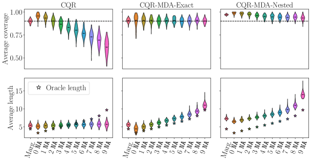
Figure 3: Average coverage (top) and length (bottom) as a function of the number of missing values (NA). The first violin plot shows the marginal coverage. $\#\rm{Tr}=500$ and $\#\rm{Cal}=250$. The marginal test set includes 2000 observations. The mask-conditional test set includes 100 individuals for each missing data pattern size.

Coverage and length by mask size. Figure 3 displays the average coverage and intervals’ length as a function of the pattern size, i.e., the performance metrics are aggregated by the masks with the same number of missing variables; the first violin plot of each panel corresponds to the marginal coverage (see Section G.2 for QR results). Note that only the pattern sizes are presented and not the patterns themselves as there are $2^{d}=1024$ possible masks. For each pattern size, 100 observations are drawn according to the distribution of $M|\text{size}(M)$ in the test set. The training and calibration sizes are respectively 500 and 250 (Figure 11 contains the results for other sizes). Figure 3 shows that:

• CQR is marginally valid (Proposition 3.3);

• CQR and QR undercover with an increasing number of missing values. This can be explained because their length nearly does not vary with the size of the missing pattern, despite having the mask concatenated with the features;

• Both versions of CQR-MDA are marginally valid (Th. 5.4) and mask(-size)-conditionally-valid (Th. 5.3);

• CQR-MDA-Exact is exactly mask(-size)-conditionally-valid (Theorem 5.3) and its length is close to the oracle ones. It has more variability for the patterns with few missing values as for these masks $\rm{Cal}^{(\text{test})}$ is smaller.

Similar experiments with 40% of missing values are available in Section G.3. Briefly, it corresponds to a setting where CP-MDA-Nested is preferable over CP-MDA-Exact as the former outputs smaller intervals and is less variable.

7.2 Semi-synthetic experiments

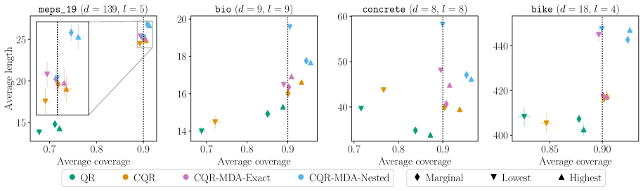
Figure 4: Validity and efficiency with missing values for 4 data sets (panels) with $d$ features, including $l$ quantitative ones in which missing values are introduced with probability 0.2. Colors represent the methods. Diamonds ($\blacklozenge$) represent marginal coverage while the patterns giving the lowest and highest mask coverage are represented with triangles ($\blacktriangledown$ and $\blacktriangle$). Vertical dotted lines represent the target coverage.

We consider 6 benchmark real data sets for regression: meps_19, meps_20, meps_21 (MEPS,, 2016), bio, bike and concrete (Dua and Graff,, 2017), where we introduce missing values in their quantitative features, each of them having a probability 0.2 of being missing (i.e. it is a MCAR mechanism), as in the synthetic experiments. Note that therefore some patterns have a low (or null) frequency of appearance in the training sets of bio and concrete. The sample sizes for training, calibration, and testing, and simulation details are provided in Section G.4, along with results for smaller training and calibration sets.

Figure 4 depicts the results by combining validity and efficiency (length) for meps_19, bio, concrete, and bike, where this graph follows the visualization used in Zaffran et al., (2022). The results for meps_20 and meps_21 are given in Section G.4, as they are similar to meps_19.

Each of the panels in Figure 4 summarizes the results for one data set, with the average coverage shown in the $x$-axis and the average length in the $y$-axis. A method is mask-conditionally-valid if all the markers of its color are at the right of the vertical dotted line (90%). The design of Figure 4 requires a different interpretation than Figure 3 (or the subsequent Figure 5). For each method we report, for the pattern having the highest (or lowest) coverage, its length and coverage. However, as this pattern may depend on the method, the length for the highest/lowest should not be directly compared between methods. We observe that:

• CQR is marginally valid (orange $\blacklozenge$, Proposition 3.3), but not MCV as the lowest mask coverage (orange $\blacktriangledown$) is far below 90% (bio, concrete, and bike data sets);

• CQR-MDA-Exact is marginally valid (purple $\blacklozenge$, Theorem 5.4). It is also exactly MCV, as the lowest (purple $\blacktriangledown$) and highest (purple $\blacktriangle$) mask coverages are about 90% (Theorem 5.3);

• CQR-MDA-Nested is marginally valid (blue $\blacklozenge$, Theorem 5.4). It is also MCV, as the lowest (blue $\blacktriangledown$) mask coverage is larger than 90% (Theorem 5.3).

7.3 Predicting the level of platelets for trauma patients

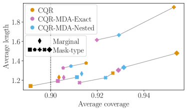
Figure 5: Average coverage and length on the TraumaBase® analysis. See the caption of Figure 4 for details. Other symbols than diamond correspond to computing the average per mask. Each individual’s prediction is obtained by using 15390 observations for training, and 7694 for calibration.

We study the applicability and robustness of CPMDA on the critical care TraumaBase® data. We focus on predicting the level of platelets of severely injured patients upon arrival at the hospital. This level is directly related to the occurrence of hemorrhagic shock and is difficult to obtain in real-time: predicting it accurately could be crucial to anticipate the need for transfusion and blood resources. In addition, this prediction task appears to be challenging as Jiang et al., (2022) achieved an average relative prediction error (${\|\hat{y}-y\|^{2}}/{\|y\|^{2}}$) that is no lower than 0.23. This highlights the need for reliable uncertainty quantification.

After applying inclusion and exclusion criteria obtained by medical doctors and following the pipeline of Sportisse et al., (2020) described in Section G.5, we left with a subset of 28855 patients and 7 features. Missing values vary from 0% to 24% by features, with a total average of 7%.

Results. The results are summarized in Figure 5, where we use different markers to denote the different masks. To ensure a fair comparison between the conformal methods, we only keep the missing patterns for which there are more than 200 individuals; this excludes 7 patterns. Finally, since we found that the vanilla QR tends to be overly conservative, we refer to Section G.5 for its results. Figure 5 shows that all conformal approaches achieve marginal coverage higher than the desired 90% level (diamonds $\blacklozenge$). Furthermore, for each mask (each set of linked markers) CQR-MDA improves coverage compared to CQR by approaching 90%, and efficiency by reducing the average length. Noticeably, for the pattern corresponding to all features observed (squares $\blacksquare$), CQR-MDA has a coverage rate above 90% while CQR is below the target level. Therefore, we believe CQR-MDA should be recommended as it improves upon the vanilla impute-then-regress+CQR approach.

8 Conclusion and perspectives

In this paper, we study the interplay between uncertainty quantification and missing values. We show that missing values introduce heteroskedasticity in the prediction task. This brings challenges on how to provide uncertainty estimators that are valid conditionally on the missing patterns, which are addressed by this work. Our analysis leaves several directions open: (1) obtaining results beyond the MCAR assumption for CP-MDA, both theoretically and numerically, (2) extending the (numerical) analysis to non-split approaches, (3) investigating the numerical performances of other conditional CP approaches (such as Sesia and Candès, (2020); Izbicki et al., (2020, 2022); Lin et al., (2021)), (4) studying the impact of the imputation on QR with finite samples. A more detailed discussion on these directions is provided in Appendix A.

Appendices

The appendices are organized as follows.

Appendix A provides a more detailed discussion on open directions and perspectives.

Appendix B describes CQR, used in the paper.

Appendix C provides an explicit description of impute-then-predict+conformalization (Section C.1), along with its proof of validity, that is the proofs for Section 3 (Section C.2).

Then, Appendix D contains the proofs for the Gaussian linear model oracle intervals presented in Section 4 (Section D.1), along with the discussion on how mean-based approaches fail (Section D.2).

Appendix E gives the general statement of CP-MDA-Exact (Section E.1), and the proofs of the validity theorems for CP-MDA-Exact (Section E.2), along with the theoretical study of CP-MDA-Nested (Section E.3).

Appendix F provides all the proofs about consistency and asymptotic conditional coverage presented in Section 6.

Finally, Appendix G contains all the details for the experimental study and additional results completing Section 7. More precisely, Section G.1 gives more details about the settings. Section G.2 contains results on synthetic data with 20% of MCAR missing values, while Section G.3 shows the results on synthetic data when the proportion of MCAR missing values is 40%. Section G.4 describes the real data sets used for the semi-synthetic experiments, and presents the remaining results. Section G.5 presents the real medical data set (TraumaBase®), the pipeline and settings used and the results obtained by QR on this data set.

Appendix A Detailed perspective discussion

First, obtaining results beyond the MCAR assumption for CP-MDA. On the numerical side, preliminary experiments show promising results, indicating CP-MDA’s robustness, but a detailed numerical study is needed. On the theoretical side, understanding the limits of CP-MDA validity is of high importance. Results without assumptions on the missingness distribution seem impossible to obtain. Even with MAR data, the task of pointwise prediction can be very challenging if the output distribution strongly depends on the pattern (Ayme et al.,, 2022). As the impossibility results of conditional validity (Lei and Wasserman,, 2014; Vovk,, 2012; Barber et al., 2021a, ), assumptions on the missing mechanism are needed.

Second, extending the (numerical) analysis to non-split approaches (e.g., based on the Jackknife) would be relevant, as it could improve the base model and therefore how the heteroskedasticity is taken into account. Note that CP-MDA can be written to take into account this splitting strategy, and thus our theoretical results on MCV would directly extend.

Third, investigating the numerical performances of other conditional CP approaches (such as Sesia and Candès, (2020); Izbicki et al., (2020, 2022); Lin et al., (2021)) within the MDA framework is of interest. In this paper, we analyze empirically the instance of CP-MDA on top of CQR as it is the simplest version of QR based CP, but the theory and motivation of this work is not specific to CQR. Exactly as CQR, none of the aforementioned methods would provide MCV if used out of the box. But if combined with CP-MDA, then all of them will be granted MCV.

Finally, while our approach is to be agnostic to the imputation chosen (similarly to CP being agnostic to the underlying model), an interesting research path is to study the impact of the imputation on QR with finite samples.

Appendix B Illustration and details on CQR (Romano et al.,, 2019) procedure

Figure 6 provides a visualization and step by step description of CQR.

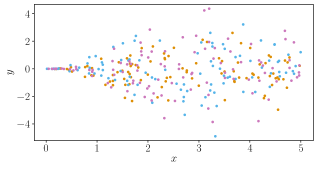
• Create a proper training set, a calibration set, and keep your test set, by randomly splitting your data set.

Step 1

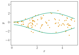
On the proper training set:

• Learn $\hat{q}_{\text{low}}$ and $\hat{q}_{\text{upp}}$

Step 2

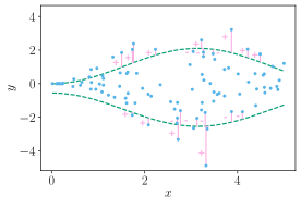
On the calibration set:

• Predict with $\hat{q}_{\text{low}}$ and $\hat{q}_{\text{upp}}$

• Get the scores
  ${{\color[rgb]{0.98828125,0.68359375,0.88671875}s^{(k)}}=\max\left\{{\color[rgb]{0.12890625,0.5703125,0.4140625}\hat{q}_{\text{low}}}\left(x^{(k)}\right)-y^{(k)},y^{(k)}-{\color[rgb]{0.12890625,0.5703125,0.4140625}\hat{q}_{\text{upp}}}\left(x^{(k)}\right)\right\}}$

• Compute the $(1-\alpha)\times(1+\frac{1}{\#\rm{Cal}})$ empirical quantile of the $s^{(k)}$, noted $\widehat{Q}_{1-\hat{\alpha}}\left(S\right)$

Step 3

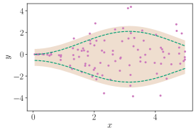
On the test set:

• Predict with $\hat{q}_{\text{low}}$ and $\hat{q}_{\text{upp}}$

• Build $\hat{C}_{\hat{\alpha}}(x)$: $[\hat{q}_{\text{low}}(x)-\widehat{Q}_{1-\hat{\alpha}}\left(S\right),\hat{q}_{\text{upp}}(x)+\widehat{Q}_{1-\hat{\alpha}}\left(S\right)]$

Figure 6: Schematic illustration of Conformalized Quantile Regression (CQR) (Romano et al.,, 2019).

Appendix C Impute-then-predict+conformalization

C.1 Description of the algorithm

Algorithm 3 SCP on impute-then-predict

1:Imputation algorithm $\mathcal{I}$, predictive algorithm $\mathcal{A}$, conformity score function $s$, significance level $\alpha$, training set $\left\{\left(X^{(1)},M^{(1)},Y^{(1)}\right),\cdots,\left(X^{(n)},M^{(n)},Y^{(n)}\right)\right\}$.

2:Prediction interval $\widehat{{C}}_{\alpha}\left(X,M\right)$.

3:Randomly split $\{1,\ldots,n\}$ into two disjoint sets $\rm{Tr}$ and $\rm{Cal}$.

4:Fit the imputation function: $\Phi(\cdot)\leftarrow\mathcal{I}\left(\left\{\left(X^{(k)},M^{(k)}\right),k\in\rm{Tr}\right\}\right)$

5:Impute the data set: $\left\{X_{\text{imp}}^{(k)}\right\}_{k=1}^{n}:=\left\{\Phi\left(X^{(k)},M^{(k)}\right)\right\}_{k=1}^{n}$

6:Fit algorithm $\mathcal{A}$: $\hat{g}(\cdot)\leftarrow\mathcal{A}\left(\left\{\left(X_{\text{imp}}^{(k)},Y^{(k)}\right),k\in\rm{Tr}\right\}\right)$

7:for $k\in\rm{Cal}$ do

8:   Set $S^{(k)}=s\left(Y^{(k)},\hat{g}\left(X_{\text{imp}}^{(k)}\right)\right)$, the conformity scores

9:end for

10:Set $\mathcal{S}_{\rm{Cal}}=\{S^{(k)},k\in\rm{Cal}\}$

11:Compute $\widehat{Q}_{1-\alpha^{\rm{SCP}}}\left(\mathcal{S}_{\rm{Cal}}\right)$, the $1-\alpha^{\rm{SCP}}$-th empirical quantile of $\mathcal{S}_{\rm{Cal}}$, with $1-\alpha^{\rm{SCP}}:=(1-\alpha)\left(1+1/\#\rm{Cal}\right)$.

12:Set $\widehat{{C}}_{\alpha}\left(X,M\right)=\left\{y\text{ such that }s\left(y,\hat{g}\circ\Phi\left(X,M\right)\right)\leq\widehat{Q}_{1-\alpha^{\rm{SCP}}}\left(\mathcal{S}_{\rm{Cal}}\right)\right\}$.

Similarly, Algorithm 1 can be written to include any underlying predictive algorithm (regression or classification) and any score function.

C.2 Proof of exchangeability after imputation

In this subsection, we provide a more formal statement of Lemma 3.2 and Proposition 3.3 in respectively Lemma C.1 and Proposition C.2. To that end, we introduce a notion of symmetrical imputation on a set $\mathcal{T}$, for $\mathcal{T}\subset\llbracket 1,n+1\rrbracket$.

Assumption A5 (Symmetrical imputation on a set $\mathcal{T}$).

For a given set of points $\{X^{(k)},M^{(k)},Y^{(k)}\}_{k\in\mathcal{T}}$ the imputation function $\Phi$ is the output of an algorithm $\mathcal{I}$ that treats the data points in $\mathcal{T}$ symmetrically: $\mathcal{I}(\{X^{(k)},M^{(k)},Y^{(k)}\}_{k\in\mathcal{T}})\overset{(d)}{=}\mathcal{I}(\{X^{(\sigma(k))},M^{(\sigma(k))},Y^{(\sigma(k))}\})_{k\in\mathcal{T}}$ conditionally to $\{X^{(k)},M^{(k)},Y^{(k)}\}_{k\in\mathcal{T}}$ and for any permutation $\sigma$ on $\llbracket 1,\#\mathcal{T}\rrbracket$.

Lemma C.1 (Imputation preserves exchangeability).

Let A1 hold. Then, for any missing mechanism, for any imputation function $\Phi$ satisfying A5, the imputed random variables $\left(\Phi\left(X^{(k)},M^{(k)}\right),M^{(k)},Y^{(k)}\right)_{k\in\mathcal{T}}$ are exchangeable.

Proposition C.2 ((Exact) validity of impute-then-predict+conformalization).

If A1 is satisfied, then we have the following three results.

1. Full CP: if A5 is satisfied for $\mathcal{T}=\llbracket 1,n+1\rrbracket$ (i.e., the imputation algorithm treats all points symmetrically), then impute-then-predict+Full CP is marginally valid. If moreover the scores are almost surely distinct, it is exactly valid.

   OR

2. Jackknife+ if A5 is satisfied for $\mathcal{T}=\llbracket 1,n+1\rrbracket$ (i.e., the imputation algorithm treats all points symmetrically), then impute-then-predict+Jackknife+ is marginally valid (of level $1-2\alpha$).

   OR

3. SCP with the split $\llbracket 1,n+1\rrbracket=\rm{Tr}\bigcup\rm{Cal}\bigcup\rm{Test}$ and if A5 is satisfied for $\mathcal{T}=\rm{Cal}\bigcup\rm{Test}$ (i.e., the imputation treats all points in $\rm{Cal}\bigcup\rm{Test}$ symmetrically) then impute-then-predict+conformalization is marginally valid. If moreover the scores are almost surely distinct, it is exactly valid.

Remark C.3 (Imputation choices for SCP).

In the latter case, for SCP, the coverage result can be derived conditionally on $\rm{Tr}$, thus the coverage results holds for: (i) any deterministic imputation function (conditionally on $\rm{Tr}$) (that is any arbitrary function of $\rm{Tr}$), or (ii) any stochastic imputation function treating $\rm{Cal}$ and $\rm{Test}$ symmetrically (iii) any combination of both.

Proof of Lemma C.1.

$\Phi$ is the output of an imputing algorithm $\mathcal{I}$ trained on $\left\{\left(X^{(k)},M^{(k)},Y^{(k)}\right)_{k\in\mathcal{T}}\right\}$.

Assume $\left(X^{(k)},M^{(k)},Y^{(k)}\right)_{k\in\mathcal{T}}$ are exchangeable (A1).

Thus, if $\mathcal{I}$ treats the data points in $\mathcal{T}$ symmetrically, $\left(\Phi(X^{(k)},M^{(k)}),M^{(k)},Y^{(k)}\right)_{k\in\mathcal{T}}$ are exchangeable (see proof of Theorem 1b in (Barber et al.,, 2022) for example).

∎

Proof of Proposition C.2.

Proposition C.2 is a consequence of Lemma C.1 with different choices of $\mathcal{T}$, that enable to apply the following results:

1. Full CP: Vovk et al., (2005), also re-stated in Barber et al., (2022)

2. Jackknife+: Barber et al., 2021b

3. SCP: Lei et al., (2018) or Papadopoulos et al., (2002) and Angelopoulos and Bates, (2023) for a generic version with any score function (note that the coverage is proved conditionally on $\rm{Tr}$).

∎

Appendix D Gaussian linear model

D.1 Distribution of $Y|(X_{\rm{obs}(m)},M)$ and oracle intervals

Proposition D.1 (Distribution of $Y|(X_{\rm{obs}(M)},M)$ (Le Morvan et al., 2020b, )).

Under 4.1, for any $m\in\{0,1\}^{d}$:

$$Y|(X_{\rm{obs}(m)},M=m)\sim\mathcal{N}\left(\tilde{\mu}^{m},\widetilde{\Sigma}^{m}\right),$$

with:

$$\tilde{\mu}^{m}= \;\beta^{T}_{\rm{obs}(m)}X_{\rm{obs}(m)}+\beta^{T}_{\mathrm{mis}(m)}\mu^{m}_{{\mathrm{mis}}|{\rm{obs}}}$$

$$\mu^{m}_{{\mathrm{mis}}|{\rm{obs}}}= \;\mu^{m}_{\mathrm{mis}(m)}+\Sigma^{m}_{\mathrm{mis}(m),\rm{obs}(m)}({\Sigma^{m}_{\rm{obs}(m),\rm{obs}(m)}})^{-1}(X_{\rm{obs}(m)}-\mu^{m}_{\rm{obs}(m)}),$$

$$\widetilde{\Sigma}^{m}= \;\beta^{T}_{\mathrm{mis}(m)}\Sigma^{m}_{{\mathrm{mis}}|{\rm{obs}}}\beta_{\mathrm{mis}(m)}+\sigma^{2}_{\varepsilon}$$

$$\Sigma^{m}_{{\mathrm{mis}}|{\rm{obs}}}= \;\Sigma^{m}_{\mathrm{mis}(m),\mathrm{mis}(m)}-\Sigma^{m}_{\mathrm{mis}(m),\rm{obs}(m)}({\Sigma^{m}_{\rm{obs}(m),\rm{obs}(m)}})^{-1}\Sigma^{m}_{\rm{obs}(m),\mathrm{mis}(m)}.$$

Proposition D.2 (Oracle intervals).

Under 4.1, for any $m\in\{0,1\}^{d}$, for any $\delta\in(0,1)$:

$$q^{Y|(X_{\rm{obs}(m)},M=m)}_{\delta} =\beta^{T}_{\rm{obs}(m)}X_{\rm{obs}(m)}+\beta^{T}_{\mathrm{mis}(m)}\mu^{m}_{\mathrm{mis}|\rm{obs}}+q^{\mathcal{N}(0,1)}_{\delta}\sqrt{\beta^{T}_{\mathrm{mis}(m)}\Sigma^{m}_{\mathrm{mis}|\rm{obs}}\beta_{\mathrm{mis}(m)}+\sigma^{2}_{\varepsilon}},$$

and the oracle predictive interval length is given by:

$$\mathcal{L}^{*}_{\alpha}(m)=2q^{\mathcal{N}(0,1)}_{1-\frac{\alpha}{2}}\sqrt{\beta^{T}_{\mathrm{mis}(m)}\Sigma^{m}_{\mathrm{mis}|\rm{obs}}\beta_{\mathrm{mis}(m)}+\sigma^{2}_{\varepsilon}}.$$ (5)

Proof.

Using multivariate Gaussian conditioning (Eaton,, 1983), for any subset of indices $L\in\llbracket 1,d\rrbracket$:

$$X_{K}|(X_{L},M)\sim\mathcal{N}(\mu^{M}_{K|L},\Sigma^{M}_{K|L}),$$ (6)

with $K=\bar{L}$ (the complement indices) and:

$$\mu^{M}_{K|L} =\mu^{M}_{K}+\Sigma^{M}_{K,L}{\Sigma^{M}_{L,L}}^{-1}(X_{L}-\mu^{M}_{L}),$$

$$\Sigma^{M}_{K|L} =\Sigma^{M}_{K,K}-\Sigma^{M}_{K,L}{\Sigma^{M}_{L,L}}^{-1}\Sigma^{M}_{L,K}.$$

Given that $Y=\beta^{T}X+\varepsilon$, with $\varepsilon\sim\mathcal{N}(0,\sigma^{2}_{\varepsilon})\perp\!\!\!\!\perp(X,M)$, the following holds:

$$Y|(X_{L},M) \overset{(d)}{=}(\beta^{T}X+\varepsilon)|(X_{L},M)\overset{(d)}{=}\beta^{T}_{L}X_{L}+(\varepsilon+\beta^{T}_{K}X_{K})|(X_{L},M)$$

and by Equation 6, $\beta^{T}_{K}X_{K}|(X_{L},M)\sim\mathcal{N}(\beta^{T}_{K}\mu^{M}_{K|L},\beta^{T}_{K}\Sigma^{M}_{K|L}\beta_{K})$, and $(\varepsilon|(X_{L},M))\sim\mathcal{N}(0,\sigma^{2}_{\varepsilon})$, and $(\beta^{T}_{K}X_{K}\perp\!\!\!\!\perp\varepsilon)|(X_{L},M)$ . Thus:

$$Y|(X_{L},M)\sim\mathcal{N}(\beta^{T}_{L}X_{L}+\beta^{T}_{K}\mu^{M}_{K|L},\beta^{T}_{K}\Sigma^{M}_{K|L}\beta_{K}+\sigma^{2}_{\varepsilon}).$$

Consequently, for any $\delta\in(0,1)$:

$$q^{Y|(X_{L},M)}_{\delta}=\beta^{T}_{L}X_{L}+\beta^{T}_{K}\mu^{M}_{K|L}+q^{\mathcal{N}(0,1)}_{\delta}\sqrt{\beta^{T}_{K}\Sigma^{M}_{K|L}\beta_{K}+\sigma^{2}_{\varepsilon}}.$$ (7)

For any pattern $m\in\{0,1\}^{d}$, applying Equation 7 with $K=\mathrm{mis}(m)=\overline{\rm{obs}(m)}$, $L=\rm{obs}(m)$, we have, for any $\delta\in(0,1)$:

$$q^{Y|(X_{\rm{obs}(m)},M=m)}_{\delta}= \beta^{T}_{\rm{obs}(m)}X_{\rm{obs}(m)}+\beta^{T}_{\mathrm{mis}(m)}\mu^{m}_{\mathrm{mis}|{\rm{obs}}}+q^{\mathcal{N}(0,1)}_{\delta}\sqrt{\beta^{T}_{\mathrm{mis}(m)}\Sigma^{m}_{{\mathrm{mis}}|{\rm{obs}}}\beta_{\mathrm{mis}(m)}+\sigma^{2}_{\varepsilon}},$$

and:

$$\mathcal{L}^{*}_{\alpha}(m)=2\times q^{\mathcal{N}(0,1)}_{1-\alpha/2}\times\sqrt{\beta^{T}_{\mathrm{mis}(m)}\Sigma^{m}_{{\mathrm{mis}}|{\rm{obs}}}\beta_{\mathrm{mis}(m)}+\sigma^{2}_{\varepsilon}},$$

with:

$$\mu^{m}_{\mathrm{mis}|\rm{obs}} =\mu^{m}_{\mathrm{mis}(m)}+\Sigma^{m}_{\mathrm{mis}(m),\rm{obs}(m)}({\Sigma^{m}_{\rm{obs}(m),\rm{obs}(m)}})^{-1}(X_{\rm{obs}(m)}-\mu^{m}_{\rm{obs}(m)}),$$

$$\Sigma^{m}_{\mathrm{mis}|\rm{obs}} =\Sigma^{m}_{\mathrm{mis}(m),\mathrm{mis}(m)}-\Sigma^{m}_{\mathrm{mis}(m),\rm{obs}(m)}({\Sigma^{m}_{\rm{obs}(m),\rm{obs}(m)}})^{-1}\Sigma^{m}_{\rm{obs}(m),\mathrm{mis}(m)}.$$

∎

D.2 Discussion on how mean-based approaches fail

Under 4.1, the Bayes predictor for a quadratic loss in presence of missing values – $\mathds{E}\left[Y |\left(X_{\rm{obs}(M)},M\right)\right]$ – is fully characterized (Le Morvan et al., 2020b, ; Le Morvan et al., 2020a, ; Ayme et al.,, 2022). Figure 7 is obtained by generating the data according to 4.1 with $d=3$, $\beta=(1,2,-1)^{T}$ and $\sigma_{\varepsilon}=1$, with multivariate Gaussian $X$ and MCAR mechanism ($X\perp\!\!\!\!\perp M$) (which is a particular case of 4.1 with $\mu^{m}\equiv\mu$ and $\Sigma^{m}\equiv\Sigma$). The left panel represents the method Oracle mean + SCP where SCP is applied on the regressor being the Bayes predictor for the mean with absolute residuals as the score function. The first violin plot represents the marginal coverage whereas the other 7 represent conditional coverage with respect to the different possible patterns: conditional on observing all the variables, on observing all the variables except $X_{1}$, except $X_{2}$ etc (see Section 7 for details on the simulation process).

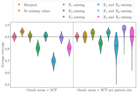
Figure 7: Calibration set contains 500 points. Test size for each pattern is of 500 individuals and for marginal is of 2000. 200 repetitions allow to display violin plots, the horizontal black line representing the mean.

SCP on a (oracle) mean regressor lacks of conditional coverage with respect to the mask.

Figure 7 (left) highlights that even with the best mean regressor (the Bayes predictor) and an homoskedastic noise, usual SCP intervals:

• over-cover when there are no missing values;

• cover less for a mask $\breve{m}$ than for a mask $\mathring{m}$ when $\mathring{m}\subset\breve{m}$ (e.g. $\mathring{m}=(1,0,0)$ only $X_{1}$ is missing, $\breve{m}=(1,1,0)$ that is $X_{1}$ and $X_{2}$ are missing);

• cover less when the most informative variable ($X_{2}$) is missing.

To tackle this issue, one could calibrate conditionally to the missing data patterns. This is in the same vein as calibrating conditionally to the categories of a categorical variable or to different groups (Romano et al.,, 2020). This strategy is not viable as there are $2^{d}$ patterns: the number of subsets grows exponentially with the dimension, implying the creation of subsets with too little data to perform the calibration. As an alternative, one could consider to perform calibration conditionally to the pattern size (e.g. when $d=3$, either 0 missing value, 1 or 2). This is possible as there are only $d$ different pattern sizes.

Calibrating by pattern size does not provide validity conditionally to the missing data patterns.

Figure 7 (right) shows the coverages of Oracle mean + SCP per pattern size where SCP is applied on the Bayes predictor for the mean and the calibration is protected by pattern size. The previous statements still hold with this strategy, even if the coverage disparities are smaller. Therefore, it is not enough to calibrate per pattern size.

Appendix E Finite sample algorithms

E.1 General statement of Algorithm 1

We provide in Algorithm 4 a general statement of CP-MDA-Exact handling any learning algorithm (both regression and classification) and any score function.

Algorithm 4 CP-MDA-Exact

1:Imputation algorithm $\mathcal{I}$, predictive algorithm $\mathcal{A}$, conformity score function $s_{g}$ paramatrized by a model $g$, significance level $\alpha$, training set $\left\{\left(X^{(k)},M^{(k)},Y^{(k)}\right)\right\}_{k=1}^{n}$, test point $\left(X^{(\text{test})},M^{(\text{test})}\right)$.

2:Prediction interval ${\widehat{C}}_{\alpha}\left(x^{(\text{test})},m^{(\text{test})}\right)$.

3:Randomly split $\{1,\ldots,n\}$ into two disjoint sets $\rm{Tr}$ and $\rm{Cal}$.

4:Fit the imputation function: $\Phi(\cdot)\leftarrow\mathcal{I}\left(\left\{\left(X^{(k)},M^{(k)}\right),k\in\rm{Tr}\right\}\right)$

5:Impute the training set: $\left\{X_{\text{imp}}^{(k)}\right\}_{k\in\rm{Tr}}:=\left\{\Phi\left(X^{(k)},M^{(k)}\right)\right\}_{k\in\rm{Tr}}$

6:Fit algorithm $\mathcal{A}$: $\hat{g}(\cdot)\leftarrow\mathcal{A}\left(\left\{\left(X_{\text{imp}}^{(k)},Y^{(k)}\right),k\in\rm{Tr}\right\}\right)$

7:// Generate an augmented calibration set:

8:$\rm{Cal^{(\text{test})}}=\left\{k\in\rm{Cal}\text{ such that }M^{(k)}\subset M^{(\text{test})}\right\}$

9:for $k\in\rm{Cal^{(\text{test})}}$ do

10:   $\widetilde{M}^{(k)}=M^{(\text{test})}$ Additional masking

11:end for

12:Augmented calibration set generated. //

13:Impute the calibration set: $\left\{X_{\text{imp}}^{(k)}\right\}_{k\in\rm{Cal^{(\text{test})}}}:=\left\{\Phi\left(X^{(k)},\widetilde{M}^{(k)}\right)\right\}_{k\in\rm{Cal^{(\text{test})}}}$

14:for $k\in\rm{Cal^{(\text{test})}}$ do

15:   Set $S^{(k)}=s_{\hat{g}}\left(Y^{(k)},X_{\text{imp}}^{(k)}\right)$, the conformity scores

16:end for

17:Set $\mathcal{S}_{\rm{Cal}}=\{S^{(k)},k\in\rm{Cal^{(\text{test})}}\}$

18:Compute $\widehat{Q}_{1-\tilde{\alpha}}\left(\mathcal{S}_{\rm{Cal}}\right)$, the $1-\tilde{\alpha}$-th empirical quantile of $\mathcal{S}_{\rm{Cal}}$, with $1-\tilde{\alpha}:=(1-\alpha)\left(1+1/\#\mathcal{S}{Cal}\right)$.

19:Set ${\widehat{C}}_{\alpha}\left(X^{(\text{test})},M^{(\text{test})}\right)=\left\{y\text{ such that }s_{\hat{g}}\left(y,\Phi\left(X^{(\text{test})},M^{(\text{test})}\right)\right)\leq\widehat{Q}_{1-\hat{\alpha}}\left(\mathcal{S}_{\rm{Cal}}\right)\right\}$.

E.2 Mask-conditional valitidy of CP-MDA-Exact

Before proving the results, we introduce a slightly stronger notion of mask-conditional-validity, when the calibration set is itself of random cardinality.

Definition E.1 (Mask-conditional-validity-random-calibration-size).

A method is mask-conditionally-valid with a random calibration size $\#\rm{Cal}$ if for any $m\in\mathcal{M}$, the lower bound is satisfied, and exactly mask-conditionally-valid if for any $m\in\mathcal{M}$, $1\leq c\leq n$, the upper bound is also satisfied:

$$1-\alpha\!\!\!\underset{\text{valid}}{\leq}\!\!\mathds{P}\left(Y^{(n+1)}\in\widehat{C}_{\alpha}\left(X^{(n+1)},m\right)|M^{(n+1)}=m,\#\rm{Cal}=c\right)\underset{\text{exactly valid}}{\leq}1-\alpha+\frac{1}{c+1}.$$

We start by proving Theorem E.2 that implies the result on CP-MDA-Exact in Theorem 5.3.

Theorem E.2.

[Conditional validity of CP-MDA-Exact with calibration of random cardinality] Assume the missing mechanism is MCAR, and that Assumptions A1, A3 and A2 hold. Then:

• CP-MDA-Exact is valid with a random calibration size $\#\rm{Cal}$ conditionally to the missing patterns;

• if the scores $S^{(k)}$ are almost surely distinct, CP-MDA-Exact is exactly mask-conditionally-valid with a random calibration size $\#\rm{Cal}$.

Proof of Theorem E.2.

Let $\rm{Tr}$ and $\rm{Cal}$ be two disjoint sets on $\llbracket 1,n\rrbracket$. Let $\hat{g}$ be some model. Given A1, the sequence $\left\{\left(X^{(k)},M^{(k)},Y^{(k)}\right)_{k\in\rm{Cal}},\left(X^{(\rm{test})},M^{(\rm{test})},Y^{(\rm{test})}\right)\right\}$ is exchangeable. Therefore, the sequence $\left\{\left(X^{(k)},Y^{(k)}\right)_{k\in\rm{Cal}},\left(X^{(\rm{test})},Y^{(\rm{test})}\right)\right\}$ is also exchangeable.

Let $m$ in $\mathcal{M}$. We define $\rm{Cal}^{m}=\left\{k\in\rm{Cal}\text{ such that }M^{(k)}\subset m\right\}$.

Let $c\in\llbracket 1,\#\rm{Cal}\rrbracket$.

As the $M\perp\!\!\!\!\perp X$ (missingness is MCAR) and $(M\perp\!\!\!\!\perp Y)|X$ (Assumption A3), then $M\perp\!\!\!\!\perp(X,Y)$, and $\#\rm{Cal}^{m}\perp\!\!\!\!\perp\left(X^{(k)},Y^{(k)}\right)_{k\in\rm{Cal}},\left(X^{(\rm{test})},Y^{(\rm{test})}\right)$. It follows that the sequence $\left\{\left(X^{(k)},Y^{(k)}\right)_{k\in{\color[rgb]{0.31640625,0.67578125,0.88671875}\rm{Cal}^{m}}},\left(X^{(\rm{test})},Y^{(\rm{test})}\right)\right\}$ is exchangeable conditionally to $\#\rm{Cal}^{m}=c$.

Similarly, $M^{(\rm{test})}\perp\!\!\!\!\perp\left(X^{(k)},Y^{(k)}\right)_{k\in\rm{Cal}},\left(X^{(\rm{test})},Y^{(\rm{test})}\right)$. Thus the sequence $\{\left(X^{(k)},M^{(\rm{test})},Y^{(k)}\right)_{k\in{\color[rgb]{0.31640625,0.67578125,0.88671875}\rm{Cal}^{m}}},\left(X^{(\rm{test})},M^{(\rm{test})},Y^{(\rm{test})}\right)\}$ is exchangeable conditionally to $\#\rm{Cal}^{m}=c$ and $M^{(\rm{test})}=m$.

Therefore, we can now invoke Proposition 3.3 in combination with Lemma 1 of Romano et al., (2020) to conclude the proof. But we can state a more rigorous version here, since in fact $\rm{Cal}^{m}$ is a random variable (as discussed in Definition E.1).

Since the algorithm $\mathcal{I}$ treats the calibration and test data points symmetrically (A5 with $\mathcal{T}=\rm{Cal}\bigcup\rm{Test}$), A5 also holds for any $\mathcal{T}^{\prime}\subset\mathcal{T}$. Therefore, by Lemma C.1 the sequence $\left\{\left(\Phi(X^{(k)},M^{(\rm{test})}),M^{(\rm{test})},Y^{(k)}\right)_{k\in\rm{Cal}^{m}},\left(\Phi(X^{(\rm{test})},M^{(\rm{test})}),M^{(\rm{test})},Y^{(\rm{test})}\right)\right\}$ is exchangeable conditionally to $\#\rm{Cal}^{m}=c$ and $M^{(\rm{test})}=m$.

The conclusion follows from usual arguments (Papadopoulos et al.,, 2002; Lei et al.,, 2018; Angelopoulos and Bates,, 2023).

Precisely, $\left\{\left(s_{\hat{g}}(Y^{(k)},\Phi(X^{(k)},M^{(\rm{test})}))\right)_{k\in\rm{Cal}^{m}},s_{\hat{g}}(Y^{(\rm{test})},\Phi(X^{(\rm{test})},M^{(\rm{test})}))\right\}$ is exchangeable conditionally to $\#\rm{Cal}^{m}=c$ and ${M^{(\rm{test})}=m}$. Therefore,

$$\mathds{P}\left(s_{\hat{g}}(Y^{(\rm{test})},\Phi(X^{(\rm{test})},M^{(\rm{test})}))\leq\widehat{Q}_{1-\tilde{\alpha}}((s_{\hat{g}}(Y^{(k)},\Phi(X^{(k)},M^{(\rm{test})})))_{k\in\rm{Cal}^{m}})\Big{|}M^{(\rm{test})}=m,\#\rm{Cal}^{m}=c\right)\geq 1-\alpha,$$

and if the $\left(\left(s_{\hat{g}}(Y^{(k)},\Phi(X^{(k)},M^{(\rm{test})}))\right)_{k\in\rm{Cal}^{m}},s_{\hat{g}}(Y^{(\rm{test})},\Phi(X^{(\rm{test})},M^{(\rm{test})}))\right)$ are almost surely distinct (i.e. have a continuous distribution) then (Lei et al.,, 2018; Romano et al.,, 2019): $\mathds{P}\left(s_{\hat{g}}(Y^{(\rm{test})},\Phi(X^{(\rm{test})},M^{(\rm{test})}))\leq\widehat{Q}_{1-\tilde{\alpha}}\big{(}(s_{\hat{g}}(Y^{(k)},\Phi(X^{(k)},M^{(\rm{test})})))_{k\in\rm{Cal}^{m}}\big{)}\Big{|}M^{(\rm{test})}=m,\#\rm{Cal}^{m}=c\right)\leq 1-\alpha+\frac{1}{c+1}.$

This proves the first two points (with respect to Definition E.1) of Theorem 5.3, by observing that $\left\{Y^{(\rm{test})}\in\widehat{C}_{\alpha}(X^{(\rm{test})},M^{(\rm{test})})\right\}=\left\{s_{\hat{g}}(Y^{(\rm{test})},\Phi(X^{(\rm{test})},M^{(\rm{test})}))\leq\widehat{Q}_{1-\tilde{\alpha}}\left(\left(s_{\hat{g}}(Y^{(k)},\Phi(X^{(k)},M^{(\rm{test})}))\right)_{k\in\rm{Cal}^{m}}\right)\right\}$.

∎

Then, the proof of Theorem 5.4 (marginal validity of the CP-MDA-Exact) is direct by marginalizing the result of Theorem 5.3. ∎

E.3 Validities of CP-MDA-Nested.

Next, we give more details on the results on CP-MDA-Nested.

E.3.1 Mask-conditional-validity of CP-MDA-Nested.

Let $m\in\mathcal{M}$.

We start by describing the links between CP-MDA-Nested and CP-MDA-Exact. CP-MDA-Exact can be re-written in the same way as CP-MDA-Nested, but keeping the subselection step of l. 8.

Indeed, first mention that the output of Algorithm 1 can be written in the following ways:

• $\widehat{C}_{\alpha}({\color[rgb]{0.7578125,0.4453125,0.6953125}X^{(\rm{test})},m^{(\rm{test})}})=\left[\hat{q}_{\frac{\alpha}{2}}\circ\Phi(X^{(\rm{test})},m^{(\rm{test})})-\widehat{Q}_{1-\tilde{\alpha}}\left(S\right);\hat{q}_{1-\frac{\alpha}{2}}\circ\Phi(X^{(\rm{test})},m^{(\rm{test})})+\widehat{Q}_{1-\tilde{\alpha}}\left(S\right)\right]$

• $\widehat{C}_{\alpha}({\color[rgb]{0.7578125,0.4453125,0.6953125}X^{(\rm{test})},m^{(\rm{test})}})=\left[\widehat{Q}_{\tilde{\alpha}}\left(\hat{q}_{\frac{\alpha}{2}}\circ\Phi(X^{(\rm{test})},m^{(\rm{test})})-S_{\rm{Cal}^{(\rm{test})}}\right);\widehat{Q}_{1-\tilde{\alpha}}\left(\hat{q}_{1-\frac{\alpha}{2}}\circ\Phi(X^{(\rm{test})},m^{(\rm{test})})+S_{\rm{Cal}^{(\rm{test})}}\right)\right]$

• $\widehat{C}_{\alpha}({\color[rgb]{0.7578125,0.4453125,0.6953125}X^{(\rm{test})},m^{(\rm{test})}})=\left[\widehat{Q}_{\tilde{\alpha}}\left(Z^{m^{(\rm{test})}}_{\frac{\alpha}{2}}\right);\widehat{Q}_{1-\tilde{\alpha}}\left(Z^{m^{(\rm{test})}}_{1-\frac{\alpha}{2}}\right)\right]$.

With $Z^{m}_{\frac{\alpha}{2}}:=\{z^{(k)}_{\frac{\alpha}{2}},k\in\rm{Cal}\text{ and }\widetilde{M}^{(k)}=m\}$, and similarly for the upper bag. Recall that we have: $z^{(k)}_{\frac{\alpha}{2}}=\hat{q}_{\frac{\alpha}{2}}\circ\Phi\left({\color[rgb]{0.12890625,0.5703125,0.4140625}x^{(\text{test})},\widetilde{m}^{(k)}}\right)-s^{(k)}.$

On the other hand, the output predictive interval of Algorithm 2 is then written as:

• ${\widehat{C}}_{\alpha}\left({\color[rgb]{0.7578125,0.4453125,0.6953125}X^{(\rm{test})},m^{(\rm{test})}}\right)=[\widehat{Q}_{\tilde{\alpha}}\left(Z_{\frac{\alpha}{2}}\right);\widehat{Q}_{1-\tilde{\alpha}}\left(Z_{1-\frac{\alpha}{2}}\right)]$.

With these notations, $Z_{\frac{\alpha}{2}}$ can be partitioned as

$$Z_{\frac{\alpha}{2}}=Z^{m}_{\frac{\alpha}{2}}\bigcup\Bigg{(}\bigcup\limits_{\widetilde{m}^{(k)}\supset m}Z^{\widetilde{m}^{(k)}}_{\frac{\alpha}{2}}\Bigg{)}.$$ (8)

With

$$Z_{\frac{\alpha}{2}} =\{Z^{(k)}_{\frac{\alpha}{2}},k\in\rm{Cal}\}$$

$$Z^{(k)}_{\frac{\alpha}{2}} =\hat{q}_{\frac{\alpha}{2}}\circ\Phi\left({\color[rgb]{0.12890625,0.5703125,0.4140625}X^{(\text{test})},\widetilde{M}^{(k)}}\right)-S^{(k)}$$

$$s^{(k)} =\max(\hat{q}_{\frac{\alpha}{2}}(x_{\text{imp}}^{(k)})-y^{(k)},y^{(k)}-\hat{q}_{1-\frac{\alpha}{2}}(x_{\text{imp}}^{(k)})).$$

The result of Algorithm 1 implies that for any mask $m\in\mathcal{M}$, we have :

$$\mathds{P}\left(Y^{(\rm{test})}\in{\widehat{C}}_{\alpha}\left({\color[rgb]{0.7578125,0.4453125,0.6953125}X^{(\rm{test})},m}\right)|M^{(\rm{test})}=m\right)\geq 1-\alpha,$$

i.e.

$$\mathds{P}\left(Y^{(\rm{test})}\notin\left[\hat{q}_{\frac{\alpha}{2}}\circ\Phi(X^{(\rm{test})},m)-\widehat{Q}_{1-\tilde{\alpha}}\left(S^{m}\right);\hat{q}_{1-\frac{\alpha}{2}}\circ\Phi(X^{(\rm{test})},m)+\widehat{Q}_{1-\tilde{\alpha}}\left(S^{m}\right)\right]|M^{(\rm{test})}=m\right) \leq\alpha.$$ (9)

Where: $Q_{1-\tilde{\alpha}}\left(S\right)$ is the $(1-\alpha)(1+1/\#S)$-quantile of $S$ and $S^{m}=\{s^{(k)}\text{ for }k\in\rm{Cal}\text{ and }\widetilde{M}^{(k)}=m\}$. Equivalently:

$$\mathds{P}\left(Y^{(\rm{test})}\in\left[\widehat{Q}_{\tilde{\alpha}}\left(Z^{m}_{\frac{\alpha}{2}}\right);\widehat{Q}_{1-\tilde{\alpha}}\left(Z^{m}_{1-\frac{\alpha}{2}}\right)\right]|M^{(\rm{test})}=m\right) \geq 1-\alpha.$$ (10)

In the following Lemma, we show that for $\tilde{m}\supset m$ the result extends under Assumption A4.

Lemma E.3.

Assume Assumption A4. For any $m\in\mathcal{M}$, for any $\tilde{m}\supset m$

$$\mathds{P}\left[\left(Y^{(\rm{test})}\in\left[\widehat{Q}_{\tilde{\alpha}}\left(Z^{\tilde{m}}_{\frac{\alpha}{2}}\right);\widehat{Q}_{1-\tilde{\alpha}}\left(Z^{\tilde{m}}_{1-\frac{\alpha}{2}}\right)\right]\right)|M^{(\rm{test})}=m\right] \geq 1-\alpha.$$ (11)

This inequality shows the conservativeness of the quantiles of the bags resulting from larger missing patterns $\tilde{m}$ than $m$ when the construction of the output of Algorithm 2.

While inequality Equation 10 is “tight” in the sense that the probability is almost exactly $1-\alpha$ (item 2 of Theorem 5.3), the proof hereafter shows that Equation 11 can be pessimistic in terms of actual coverage, as one may have $\mathds{P}[(Y^{(\rm{test})}{\color[rgb]{0.84375,0.515625,0.14453125}\notin}[\widehat{Q}_{\tilde{\alpha}}(Z^{\tilde{m}}_{\frac{\alpha}{2}});\widehat{Q}_{1-\tilde{\alpha}}(Z^{\tilde{m}}_{1-\frac{\alpha}{2}})])|M^{(\rm{test})}=m]\ll\alpha$.

More precisely, we have the following inequality:

$$\leavevmode\resizebox{433.62pt}{}{ ${\mathds{E}}\left[\mathds{P}\left(Y^{(\rm{test})}\notin\left[\hat{q}_{\frac{\alpha}{2}}\circ\Phi(X^{(\rm{test})},\tilde{m})-\widehat{Q}_{1-\tilde{\alpha}}\left(S^{\tilde{m}}\right);\hat{q}_{1-\frac{\alpha}{2}}\circ\Phi(X^{(\rm{test})},\tilde{m})+\widehat{Q}_{1-\tilde{\alpha}}\left(S^{\tilde{m}}\right)\right]\bigg{|}M^{(\rm{test})}=m,X^{(\rm{test})}_{\rm{obs}(m)}\right)\bigg{|}M^{(\rm{test})}=m\right]\leq\alpha$ }.$$ (12)

The interpretation of that Lemma is that the intervals resulting from the prediction on $x^{\rm{test}},\tilde{m}$ (more data hidden) and corrected with the residuals of the calibration points $(X^{k},M^{k}=\tilde{m},Y^{k})$ have a larger probability of containing $Y^{\rm{test}}$, conditionally to $X_{\rm{obs}(m)}$ than the interval built using prediction on $x^{\rm{test}},m$ (more data available) and corrected with the residuals of the calibration points $(X^{k},M^{k}=m,Y^{k})$ (more data available)

Proof of Lemma E.3.

We start by invoking Equation 9 for $\tilde{m}$:

$$\mathds{P}\left(Y^{(\rm{test})}\notin\left[\hat{q}_{\frac{\alpha}{2}}\circ\Phi(X^{(\rm{test})},\tilde{m})-\widehat{Q}_{1-\tilde{\alpha}}\left(S^{\tilde{m}}\right);\hat{q}_{1-\frac{\alpha}{2}}\circ\Phi(X^{(\rm{test})},\tilde{m})+\widehat{Q}_{1-\tilde{\alpha}}\left(S^{\tilde{m}}\right)\right]|M^{(\rm{test})}=\tilde{m}\right)\leq\alpha.$$ (13)

Consequently, by the tower property of conditional expectations:

$$\leavevmode\resizebox{433.62pt}{}{ $\mathds{E}\left[\mathds{P}\left(Y^{(\rm{test})}\notin\left[\hat{q}_{\frac{\alpha}{2}}\circ\Phi(X^{(\rm{test})},\tilde{m})-\widehat{Q}_{1-\tilde{\alpha}}\left(S^{\tilde{m}}\right);\hat{q}_{1-\frac{\alpha}{2}}\circ\Phi(X^{(\rm{test})},\tilde{m})+\widehat{Q}_{1-\tilde{\alpha}}\left(S^{\tilde{m}}\right)\right]\bigg{|}M^{(\rm{test})}=\tilde{m},S^{(\tilde{m})},X^{(\rm{test})}_{\rm{obs}(\tilde{m})}\right)\bigg{|}M^{(\rm{test})}=\tilde{m}\right]\leq\alpha$ }.$$ (14)

Observe that $\hat{q}_{\frac{\alpha}{2}}\circ\Phi(X^{(\rm{test})},\tilde{m})-\widehat{Q}_{1-\tilde{\alpha}}\left(S^{\tilde{m}}\right)$ is $\{M^{(\rm{test})}=\tilde{m},S^{(\tilde{m})},X^{(\rm{test})}_{\rm{obs}(\tilde{m})}\}$-measurable.

Moreover, by Assumption A4, we have that for any $\delta\in[0,0.5]$:

$$q_{1-\delta/2}^{Y|(X_{\rm{obs}\left(m\right)},M=m)}\leq q_{1-\delta/2}^{Y|(X_{\rm{obs}\left(\widetilde{m}\right)},M=\widetilde{m})}$$ (15)

$$q_{\delta/2}^{Y|(X_{\rm{obs}\left({m}\right)},M={m})}\geq q_{\delta/2}^{Y|(X_{\rm{obs}\left(\widetilde{m}\right)},M=\widetilde{m})}.$$ (16)

In other words the conditional distribution of $Y$ given $X_{\rm{obs}({\widetilde{m}})}$ and $M={\widetilde{m}}$ “stochastically dominates” the conditional distribution of $Y$ given $X_{\rm{obs}({m})}$ and $M={m}$.

We thus have, with $F_{Z}$ denoting the cumulative distribution function of $Z$: $F_{Y|(X_{\rm{obs}\left(\widetilde{m}\right)},M=\widetilde{m})}$ the cumulative distribution function of $Y|(X_{\rm{obs}\left(\widetilde{m}\right)},M=\widetilde{m})$:

$$\mathds{P}\left(Y^{(\rm{test})}\notin\left[\hat{q}_{\frac{\alpha}{2}}\circ\Phi(X^{(\rm{test})},\tilde{m})-\widehat{Q}_{1-\tilde{\alpha}}\left(S^{\tilde{m}}\right);\hat{q}_{1-\frac{\alpha}{2}}\circ\Phi(X^{(\rm{test})},\tilde{m})+\widehat{Q}_{1-\tilde{\alpha}}\left(S^{\tilde{m}}\right)\right]\bigg{|}M^{(\rm{test})}=\tilde{m},S^{(\tilde{m})},X^{(\rm{test})}_{\rm{obs}(\tilde{m})}\right)$$

$$=1-\left[F_{Y|(X_{\rm{obs}\left(\widetilde{m}\right)},M=\widetilde{m})}\left(\hat{q}_{1-\frac{\alpha}{2}}\circ\Phi(X^{(\rm{test})},\tilde{m})+\widehat{Q}_{1-\tilde{\alpha}}(S^{\tilde{m}})\right)-F_{Y|(X_{\rm{obs}\left(\widetilde{m}\right)},M=\widetilde{m})}\left(\hat{q}_{\frac{\alpha}{2}}\circ\Phi(X^{(\rm{test})},\tilde{m})-\widehat{Q}_{1-\tilde{\alpha}}(S^{\tilde{m}})\right)\right]$$

$$\overset{(i)}{\geq}1-\left[F_{Y|(X_{\rm{obs}\left({m}\right)},M={m})}\left(\hat{q}_{1-\frac{\alpha}{2}}\circ\Phi(X^{(\rm{test})},\tilde{m})+\widehat{Q}_{1-\tilde{\alpha}}(S^{\tilde{m}})\right)-F_{Y|(X_{\rm{obs}\left({m}\right)},M={m})}\left(\hat{q}_{\frac{\alpha}{2}}\circ\Phi(X^{(\rm{test})},\tilde{m})-\widehat{Q}_{1-\tilde{\alpha}}(S^{\tilde{m}})\right)\right]$$

$$=\mathds{P}\left(Y^{(\rm{test})}\notin\left[\hat{q}_{\frac{\alpha}{2}}\circ\Phi(X^{(\rm{test})},\tilde{m})-\widehat{Q}_{1-\tilde{\alpha}}\left(S^{\tilde{m}}\right);\hat{q}_{1-\frac{\alpha}{2}}\circ\Phi(X^{(\rm{test})},\tilde{m})+\widehat{Q}_{1-\tilde{\alpha}}\left(S^{\tilde{m}}\right)\right]\bigg{|}M^{(\rm{test})}=m,S^{(\tilde{m})},X^{(\rm{test})}_{\rm{obs}(m)}\right).$$ (17)

At (i) we use (16) $F_{Y|(X_{\rm{obs}\left({m}\right)},M={m})}(\hat{q}_{\frac{\alpha}{2}}\circ\Phi(X^{(\rm{test})},\tilde{m})-\widehat{Q}_{1-\tilde{\alpha}}(S^{\tilde{m}}))\leq F_{Y|(X_{\rm{obs}\left(\widetilde{m}\right)},M=\widetilde{m})}(\hat{q}_{\frac{\alpha}{2}}\circ\Phi(X^{(\rm{test})},\tilde{m})-\widehat{Q}_{1-\tilde{\alpha}}(S^{\tilde{m}}))$, and (15): $F_{Y|(X_{\rm{obs}\left({m}\right)},M={m})}(\hat{q}_{1-\frac{\alpha}{2}}\circ\Phi(X^{(\rm{test})},\tilde{m})+\widehat{Q}_{1-\tilde{\alpha}}(S^{\tilde{m}}))\geq F_{Y|(X_{\rm{obs}\left(\widetilde{m}\right)},M=\widetilde{m})}(\hat{q}_{1-\frac{\alpha}{2}}\circ\Phi(X^{(\rm{test})},\tilde{m})+\widehat{Q}_{1-\tilde{\alpha}}(S^{\tilde{m}}))$ by A4. Remark that here we assume that $\left(\hat{q}_{1-\frac{\alpha}{2}}\circ\Phi(X^{(\rm{test})},\tilde{m})+\widehat{Q}_{1-\tilde{\alpha}}(S^{\tilde{m}})\right)\geq\rm{median}(Y^{(\rm{test})}|(X^{(\rm{test})}_{\rm{obs}\left(\widetilde{m}\right)},M={\tilde{m}})$ and $\left(\hat{q}_{\frac{\alpha}{2}}\circ\Phi(X^{(\rm{test})},\tilde{m})-\widehat{Q}_{1-\tilde{\alpha}}(S^{\tilde{m}})\right)\leq\rm{median}(Y^{\rm{test}}|(X^{(\rm{test})}_{\rm{obs}\left(\widetilde{m}\right)},M=\widetilde{m})$.

We obtain Equation 12 in Lemma E.3 by plugging (17) in (14), then Equation 11 by the tower property. ∎

Theorem E.4.

Assume the missing mechanism is MCAR, and that Assumptions A1, A3 and A2 hold. Additionally Assumption A4 is satisfied.

Consider the partition described in Equation 8, and consider CP-MDA-Nested running on a test point with missing pattern $m^{(\rm{test})}$, with any of the following outputs, instead of l. 18 ${\widehat{C}}_{\alpha}\left({\color[rgb]{0.7578125,0.4453125,0.6953125}x^{(\text{test})},m^{(\text{test})}}\right)=[\widehat{Q}_{\tilde{\alpha}}\left(Z_{\frac{\alpha}{2}}\right);\widehat{Q}_{1-\tilde{\alpha}}\left(Z_{1-\frac{\alpha}{2}}\right)]$:

1. ${\widehat{C}}_{\alpha}\left({\color[rgb]{0.7578125,0.4453125,0.6953125}x^{(\text{test})},m^{(\text{test})}}\right)=[\widehat{Q}_{\tilde{\alpha}}(Z^{\tilde{m}}_{\frac{\alpha}{2}});\widehat{Q}_{1-\tilde{\alpha}}(Z^{\tilde{m}}_{1-\frac{\alpha}{2}})]$ where $\tilde{m}\supset m^{(\rm{test})}$ is an arbitrary choice.

2. ${\widehat{C}}_{\alpha}\left({\color[rgb]{0.7578125,0.4453125,0.6953125}x^{(\text{test})},m^{(\text{test})}}\right)=[\widehat{Q}_{\tilde{\alpha}}(Z^{\hat{m}}_{\frac{\alpha}{2}});\widehat{Q}_{1-\tilde{\alpha}}(Z^{\hat{m}}_{1-\frac{\alpha}{2}})]$ where $\hat{m}$ is a randomly selected pattern in $\{\tilde{m},\tilde{m}\supset m^{(\rm{test})}\}$, possibly with varying probability depending on the cardinality of the sets $Z^{\tilde{m}}_{\alpha/2}$ .

Then the resulting algorithm is mask-conditionally-valid.

Proof of Theorem E.4.

The proof immediately follows from Equation 11, and gives the result without difficulty for any arbitrary pattern or random variable independent of all other randomness.

Extension to a choice that involves the cardinality of the sets $Z^{\tilde{m}}_{\alpha/2}$, leveraging the independence between these cardinals and the coverage properties (same as in the proof of Theorem E.2). ∎

Then, the proof of Theorem 5.4 (marginal validity of the CP-MDA-Nested) is direct by marginalizing the result of Theorem E.4. ∎

Appendix F Infinite data results

Proposition 6.1 ($\ell_{\beta}$-consistency of an universal learner).

Let $\beta\in[0,1]$. If $X$ admits a density on $\mathcal{X}$, then, for almost all imputation function $\Phi\in\mathcal{F}^{I}_{\infty}$, the function $g^{*}_{{\ell_{\beta}},\Phi}\circ\Phi$ is Bayes optimal for the pinball risk of level $\beta$.

Proof of Proposition 6.1.

The proof starts in the exact same way than Le Morvan et al., (2021), based on their Lemmas A.1 and A.2. For completeness, we copy here the statements of these lemmas without their proof and rewrite the two first parts of the main proof.

Let $\Phi$ be an imputation function such that for each missing data pattern $m$, $\phi^{m}\in\mathcal{C}^{\infty}\left(\mathds{R}^{|\rm{obs}(m)|},\mathds{R}^{|\mathrm{mis}(m)|}\right)$.

Lemma F.1 (Lemma A.1 in Le Morvan et al., (2021)).

Let $\phi^{m}\in\mathcal{C}^{\infty}\left(\mathds{R}^{|\rm{obs}(m)|},\mathds{R}^{|\mathrm{mis}(m)|}\right)$ be the imputation function for missing data pattern $m$, and let $\mathcal{M}^{m}=\left\{x\in\mathds{R}^{d}:x_{\mathrm{mis}(m)}=\phi^{m}\left(x_{\rm{obs}((m))}\right)\right\}$. For all $m$, $\mathcal{M}^{m}$ is an $|\rm{obs}((m))|$-dimensional manifold.

In Lemma F.1, $\mathcal{M}^{m}$ represents the manifold in which the data points are sent once imputed by $\phi^{m}$. Lemma F.1 states that this manifold is of dimension $|\rm{obs}(m)|$.

Lemma F.2 (Lemma A.2 in Le Morvan et al., (2021)).

Let $m$ and $m^{\prime}$ be two distinct missing data patterns with the same number of missing (resp. observed) values $|\mathrm{mis}|$ (resp $|\rm{obs}|$). Let $\phi^{m}\in\mathcal{C}^{\infty}\left(\mathds{R}^{|\rm{obs}(m)|},\mathds{R}^{|\mathrm{mis}(m)|}\right)$ be the imputation function for missing data pattern $m$, and let $\mathcal{M}^{m}=\left\{x\in\mathds{R}^{d}:x_{\mathrm{mis}(m)}=\phi^{m}\left(x_{\rm{obs}(m)}\right)\right\}$. We define similarly $\Phi^{\left(m^{\prime}\right)}$ and $\mathcal{M}^{\left(m^{\prime}\right)}$. For almost all imputation functions $\phi^{m}$ and $\Phi^{\left(m^{\prime}\right)}$,

$$\operatorname{dim}\left(\mathcal{M}^{m}\cap\mathcal{M}^{\left(m^{\prime}\right)}\right)=\begin{cases}0&\text{ if }|\mathrm{mis}|>\frac{d}{2}\\ d-2|\mathrm{mis}|&\text{ otherwise. }\end{cases}$$

Note that, as by Lemma F.1 $\operatorname{dim}\left(\mathcal{M}^{m}\right)=\operatorname{dim}\left(\mathcal{M}^{(m^{\prime})}\right)=|\rm{obs}|=d-|\mathrm{mis}|$, Lemma F.2 states that $\operatorname{dim}\left(\mathcal{M}^{m}\cap\mathcal{M}^{\left(m^{\prime}\right)}\right)\leq\operatorname{dim}\left(\mathcal{M}^{m}\right)=\operatorname{dim}\left(\mathcal{M}^{(m^{\prime})}\right)$.

Now, to prove Proposition 6.1 the missing data patterns are ordered as in Le Morvan et al., (2021): the first one will be the one in which all the variables are missing, while the last one will be the one in which all the variables are observed. For two data patterns with the same number of missing variables, the ordering is picked at random. We denote by $m(i)$ the $i$-th missing data pattern according to this ordering.

We are going to build a function $g_{\Phi}$ which, composed with $\Phi$, will reach the $\ell$-Bayes risk.

For each missing data pattern, and starting by $m(1)$ of all variables missing, we can define $g_{\Phi}$ on the data points from the current missing data pattern. More precisely, for each $i$, $g_{\Phi}$ is built for every imputed data point belonging to $\mathcal{M}^{(m(i))}$ except for those already considered in previous steps (one imputed data point can belong to multiple manifolds):

$$\forall Z=\Phi(X,M)\in\mathcal{M}^{(m(i))}\backslash\bigcup_{k<i}\mathcal{M}^{(m(k))},\quad g^{\star}(Z)=\tilde{f}^{\star}(\widetilde{X})$$

That is, $g_{\Phi}\circ\Phi(X,M)$ will equal $\tilde{f}^{*}(X,M)$ except possibly if $\Phi(X,M)=\Phi(\tilde{Y})$ for some $\tilde{Y}$ that has more missing values than $X,M$. Therefore, for each missing data pattern $m(i)$, $g_{\Phi}\circ\Phi$ equals $\tilde{f}^{*}$ except on $\bigcup_{k<i}\mathcal{M}^{(m(k))}$. The question that remains is: what is the dimension of $\mathcal{M}^{(m(i))}\bigcap\left(\bigcup_{k<i}\mathcal{M}^{(m(k))}\right)$, these points for which there is no necessarily equality between $g_{\Phi}\circ\Phi$ and $\tilde{f}^{*}$. First, note that $\mathcal{M}^{(m(i))}\bigcap\left(\bigcup_{k<i}\mathcal{M}^{(m(k))}\right)=\bigcup_{k<i}\left(\mathcal{M}^{(m(i))}\bigcap\mathcal{M}^{(m(k))}\right)$. For each space in this reunion, there are two cases:

• either $|\rm{obs}(m(k))|<|\rm{obs}(m(i))|$: using Lemma F.1, $\operatorname{dim}\left(\mathcal{M}^{(m(k))}\right)=|\rm{obs}(m(k))|<|\rm{obs}(m(i))|=\operatorname{dim}\left(\mathcal{M}^{(m(i))}\right)$. Thus, $\mathcal{M}^{(m(i))}\bigcap\mathcal{M}^{(m(k))}$ is of measure zero in $\mathcal{M}^{(m(i))}$.

• either $|\rm{obs}(m(k))|=|\rm{obs}(m(i))|$: using Lemma F.2, $\mathcal{M}^{(m(i))}\bigcap\mathcal{M}^{(m(k))}$ is of dimension 0 or smaller than $\operatorname{dim}\left(\mathcal{M}^{(m(i))}\right)$, thus it is of measure zero in $\mathcal{M}^{(m(i))}$.

Therefore, the set of data points for which $g_{\Phi}\circ\Phi$ does not equal the oracle is of measure 0 for each missing data pattern.

Let $\beta\in[0,1]$. We can now write down the $\ell_{\beta}$-risk of this built function:

$$\mathds{E}\left[\ell_{\beta}\left(Y,g^{*}\circ\Phi(X,M)\right)\right] =\mathds{E}\left[\rho_{\beta}\left(Y-g^{*}\circ\Phi(X,M)\right)\right]$$

$$=\mathds{E}\left[\rho_{\beta}\left(Y-\tilde{f^{*}}(X,M)+\tilde{f^{*}}(X,M)-g^{*}\circ\Phi(X,M)\right)\right]$$

$$(i) \leq\mathds{E}\left[\rho_{\beta}\left(Y-\tilde{f^{*}}(X,M)\right)\right]+\mathds{E}\left[\rho_{\beta}\left(\tilde{f^{*}}(X,M)-g^{*}\circ\Phi(X,M)\right)\right]$$

$$\leq\mathcal{R}_{\ell_{\beta}}^{*}+\mathds{E}\left[\rho_{\beta}\left(\tilde{f^{*}}(X,M)-g^{*}\circ\Phi(X,M)\right)\right],$$

where $(i)$ holds thanks to the shape of $\rho_{\beta}$. For any $w\in\mathds{R}$ and any $\lambda\in\mathds{R}_{+}$:

$$\rho_{\beta}\left(\lambda w\right) =\beta\lambda|w|\mathds{1}_{w\geq 0}+(1-\beta)\lambda|w|\mathds{1}_{w\leq 0}$$

$$\rho_{\beta}\left(\lambda w\right) =\lambda\rho_{\beta}\left(w\right).$$

Furthermore, $\rho_{\beta}$ is convex, thus for any $(u,v)\in\mathds{R}^{2}$:

$$\rho_{\beta}\left(\frac{1}{2}u+\frac{1}{2}v\right) \leq\frac{1}{2}\rho_{\beta}(u)+\frac{1}{2}\rho_{\beta}(v)$$

$$\frac{1}{2}\rho_{\beta}\left(u+v\right) \leq\frac{1}{2}\rho_{\beta}(u)+\frac{1}{2}\rho_{\beta}(v)$$

$$\rho_{\beta}\left(u+v\right) \leq\rho_{\beta}(u)+\rho_{\beta}(v).$$

As $\tilde{f^{*}}$ and $g^{*}\circ\Phi$ are equals almost everywhere on each missing subspace, $\mathds{E}\left[\rho_{\beta}\left(\tilde{f^{*}}(X,M)-g^{*}\circ\Phi(X,M)\right)\right]=0$. Indeed, decomposing by pattern one can write:

$$\mathds{E}\left[\rho_{\beta}\left(\tilde{f^{*}}(X,M)-g^{*}\circ\Phi(X,M)\right)\right] =\sum_{M=m}\mathds{P}(M=m)\mathds{E}\left[\rho_{\beta}\left(\tilde{f^{*}}(X,M)-g^{*}\circ\Phi(X,M)\right)|M=m\right]$$

and thus by equality almost everywhere for each pattern every term in this sum is null.

Therefore one obtains:

$$\mathds{E}\left[\ell_{\beta}\left(Y,g^{*}\circ\Phi(X,M)\right)\right]\leq\mathcal{R}_{\ell_{\beta}}^{*}.$$

Thus:

$$\mathds{E}\left[\ell_{\beta}\left(Y,g^{*}\circ\Phi(X,M)\right)\right]=\mathcal{R}_{\ell_{\beta}}^{*},$$

and $g^{*}\circ\Phi$ is Bayes optimal. This implies that $\mathcal{R}_{\ell_{\beta},\Phi}^{*}=\mathcal{R}_{\ell_{\beta}}^{*}$. Thus, a universally consistent algorithm learning $g_{\Phi}$ chained with $\Phi$ will lead to a Bayes consistent function. ∎

Proof of Corollary 6.2.

Corollary 6.2 states that “For any missing mechanism, for almost all imputation function $\Phi\in\mathcal{F}^{I}_{\infty}$, if $F_{Y|(X_{\rm{obs}(M)},M)}$ is continuous, a universally consistent quantile regressor trained on the imputed data set yields asymptotic conditional coverage.”.

Let $\beta\in[0,1]$.

Remark that Proposition 6.1 states that for any missing mechanism, for almost all imputation function $\Phi\in\mathcal{F}^{I}_{\infty}$ a universally consistent quantile regressor trained on the imputed data set achieves the Bayes risk asymptotically. We will thus show that any $\ell_{\beta}$-Bayes predictor $f_{\beta}^{*}$ (any function achieving the $\ell_{\beta}$-Bayes-risk) is such that $\mathds{P}(Y\leq f_{\beta}^{*}(X,M)|X_{\rm{obs}(M)},M)=\beta$ if $F_{Y|(X_{\rm{obs}(M)},M)}$ is continuous. Therefore, any two Bayes predictors $f_{\alpha/2}^{*}$ and $f_{1-\alpha/2}^{*}$ form an interval $[f_{\alpha/2}^{*}(X,M);f_{1-\alpha/2}^{*}(X,M)]$ that achieves conditional coverage (conditionally to $X_{\rm{obs}(M)}$ and $M$).

Let $f_{\beta}^{*}$ be a $\ell_{\beta}$-Bayes predictor. Then:

$$f_{\beta}^{*}\in\operatorname*{arg\,min}_{f:\mathcal{X}\times\mathcal{M}\rightarrow\mathds{R}} \mathds{E}\left[\rho_{\beta}\left(Y-f\left(X,M\right)\right)\right]$$

$$= \mathds{E}\left[\mathds{E}\left[\rho_{\beta}\left(Y-f\left(X,M\right)\right)|X_{\rm{obs}(M)},M\right]\right].$$

Let $(x,m)\in\mathcal{X}\times\mathcal{M}$. Denote $H_{x,m}(z):=\mathds{E}\left[\rho_{\beta}\left(Y-z\right)|X_{\rm{obs}(M)}=x_{\rm{obs}(m)},M=m\right]$. As $Y\neq z$ almost surely, we have:

$$H^{\prime}_{x,m}(z) =\mathds{E}\left[-\rho^{\prime}_{\beta}\left(Y-z\right)|X_{\rm{obs}(M)}=x_{\rm{obs}(m)},M=m\right]$$

$$=\mathds{E}\left[-(-\beta\mathds{1}_{Y-z\geq 0}+(1-\beta)\mathds{1}_{Y-z\leq 0})|X_{\rm{obs}(M)}=x_{\rm{obs}(m)},M=m\right]$$

$$=\mathds{E}\left[\beta\mathds{1}_{Y\geq z}-(1-\beta)\mathds{1}_{Y\leq z}|X_{\rm{obs}(M)}=x_{\rm{obs}(m)},M=m\right]$$

$$=\beta\mathds{P}\left(Y\geq z|X_{\rm{obs}(M)}=x_{\rm{obs}(m)},M=m\right)-(1-\beta)\mathds{P}\left(Y\leq z|X_{\rm{obs}(M)}=x_{\rm{obs}(m)},M=m\right)$$

$$=\beta\left(1-\mathds{P}\left(Y\leq z|X_{\rm{obs}(M)}=x_{\rm{obs}(m)},M=m\right)\right)-(1-\beta)\mathds{P}\left(Y\leq z|X_{\rm{obs}(M)}=x_{\rm{obs}(m)},M=m\right)$$

$$H^{\prime}_{x,m}(z) =\beta-\mathds{P}\left(Y\leq z|X_{\rm{obs}(M)}=x_{\rm{obs}(m)},M=m\right).$$

Therefore $H^{\prime}_{x,m}(z)\leq 0$ if and only if $\beta\leq\mathds{P}\left(Y\leq z|X_{\rm{obs}(M)}=x_{\rm{obs}(m)},M=m\right)$.

Thus, $z$ minimizes $H_{x,m}$ if and only if $\beta=\mathds{P}\left(Y\leq z|X_{\rm{obs}(M)}=x_{\rm{obs}(m)},M=m\right)$.

If $F_{Y|(X_{\rm{obs}(M)},M)}$ is continuous, there exists at least a solution, that might not be unique if it is not additionally strictly increasing. Therefore, if $F_{Y|(X_{\rm{obs}(M)},M)}$ is continuous, all the $\ell_{\beta}$-Bayes predictors can be written as $f_{\beta}^{*}(x,m)=q_{x,m}$ with $\mathds{P}\left(Y\leq q_{x,m}|X_{\rm{obs}(M)}=x_{\rm{obs}(m)},M=m\right)=\mathds{P}\left(Y\leq f_{\beta}^{*}(x,m)|X_{\rm{obs}(M)}=x_{\rm{obs}(m)},M=m\right)=\beta$.

∎

Appendix G Experimental study

G.1 Settings detail

Quantile Neural Network.

The architecture and optimization of the Quantile Neural Network used in the experiments is taken from Sesia and Romano, (2021) (their code is freely available). This is the description provided in the original paper of the neural network: “The network is composed of three fully connected layers with a hidden dimension of 64, and ReLU activation functions. We use the pinball loss to estimate the conditional quantiles, with a dropout regularization of rate 0.1. The network is optimized using Adam Kingma and Ba, (2014) with a learning rate equal to 0.0005. We tune the optimal number of epochs by cross validation, minimizing the loss function on the hold-out data points; the maximal number of epochs is set to 2000.”

G.2 Gaussian linear results

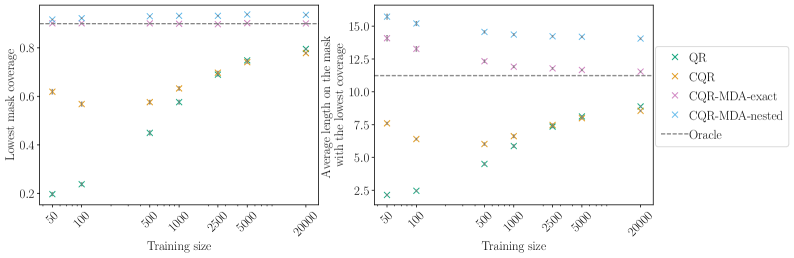
Figure 8: Coverage and interval’s length for the mask leading to the lowest coverage. Model is NN. Calibration size fixed to 1000. The mask is concatenated in the features. Data is imputed using Iterative Ridge. 100 repetitions allow to display error bars, corresponding to standard error.

Figure 9 is the analogous of Figure 8, but by evaluating the performances on the mask leading to the highest coverage.

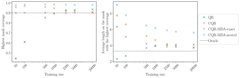
Figure 9: Coverage and interval’s length for the mask leading to the highest coverage. See caption of Figure 8 for the setting.

Hereafter, we present in Figure 10 the exact same figure than Figure 3 but with a panel (the first) for vanilla QR. The 3 other methods are displayed again to facilitate the comparison.

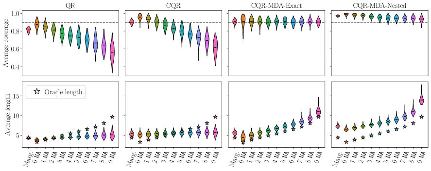
Figure 10: Average coverage (top) and length (bottom) as a function of the pattern size, i.e. the number of missing values (NA). First violin plot corresponds to marginal coverage. Stars correspond to the oracle length. Settings are: model is NN, train size is 500, calibration size is 250. The marginal test set includes 2000 observations. The conditional test set includes 100 individuals for each possible missing data pattern size. The mask is concatenated to the features. Data is imputed using Iterative Ridge. 100 repetitions are performed.

Finally, Figure 11 is the analogous of Figure 10, but for a training set containing 1000 observations and a calibration set containing 500 observations.

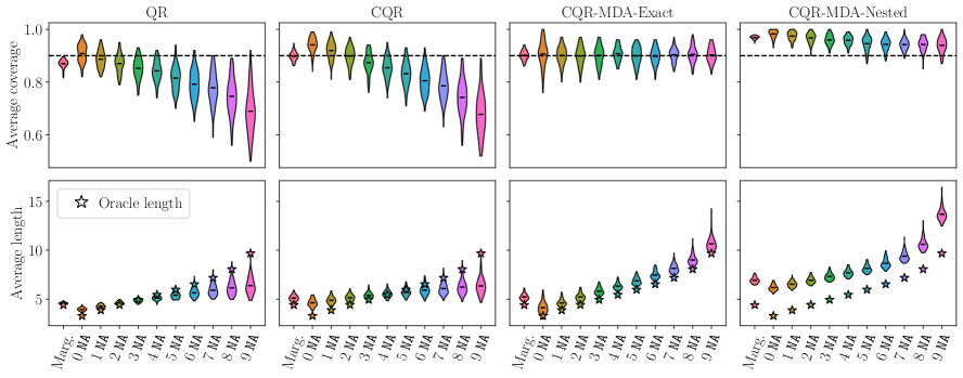
Figure 11: Model is NN. Train size is 1000. Calibration size fixed to 500. The marginal test set includes 2000 observations. The conditional test set includes 100 individuals for each possible missing data pattern size. The mask is concatenated in the features. Data is imputed using Iterative Ridge. 100 repetitions are performed.

G.3 Higher proportion of missing values

We present synthetic experiments where the proportion of MCAR missing values is of 40% (instead of 20% in Figure 3). Except from this, the settings are exactly the same than the ones of Figure 3. Precisely, the data is generated with $d=10$ according to 4.1, with $X\sim\mathcal{N}\left(\mu,\Sigma\right)$, $\mu=(1,\cdots,1)^{T}$ and $\Sigma=\varphi(1,\cdots,1)^{T}(1,\cdots,1)+(1-\varphi)I_{d}$, $\varphi=0.8$, Gaussian noise $\varepsilon\sim\mathcal{N}(0,1)$ and the following regression coefficients $\beta=(1,2,-1,3,-0.5,-1,0.3,1.7,0.4,-0.3)^{T}$. For each pattern size, 100 observations are drawn according to the distribution of $M|\text{size}(M)$ in the test set. The training and calibration sizes are respectively 500 and 250. The experiment is repeated 100 times. The results are displayed in Figure 12.

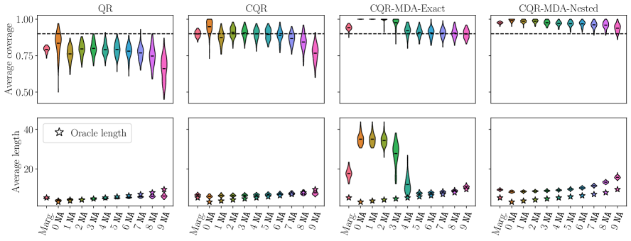
Figure 12: Same caption than Figure 10.

Interestingly, although expected, these experiments lead CP-MDA-Exact to frequently output infinite intervals. This is because the subsampling step with few calibration data – with respect to the dimension and proportion of missing values – reached a point where there are not enough observations for CP-MDA-Exact to calibrate accurately for some patterns.

To compare CP-MDA-Exact and CP-MDA-Nested in this setting, Figure 12 is obtained by replacing the infinite intervals by $\underset{k\in\mathrm{Tr}\cup\mathrm{Cal}}{\text{max}}y^{(k)}-\underset{k\in\rm{Tr}\cup\rm{Cal}}{\text{min}}y^{(k)}$. It highlights that CP-MDA-Exact is less efficient (i.e. outputs larger intervals) than CP-MDA-Nested for patterns with less than 4 NAs. With a smaller calibration set or a higher proportion of missing values, this effect would be amplified and generalized to more patterns. Figure 12 also emphasizes that CP-MDA-Exact leads to more coverage variability than CP-MDA-Nested, on the patterns for which CP-MDA-Exact does not almost surely cover.

G.4 Semi-synthetic experiments

In the semi-synthetic experiments, two settings are examined: one where the training size is small in comparison to the number of parameters of the Neural Network – “Medium” –, and one where the training size is even smaller so that some masks have a really low (or null) frequency of appearance in the training set – “Small”. In both cases, the calibration size is approximately half the training size. Figure 4 presented the results for the “Medium” case.

Table 1: Semi-synthetic settings: training and calibration sizes for each of the 6 data sets depending on the setting.

		meps_19	meps_20	meps_21	bio	bike	concrete
		$d=139$, $l=5$	$d=139$, $l=5$	$d=139$, $l=5$	$d=9$, $l=9$	$d=18$, $l=4$	$d=8$, $l=8$
		$n=15785$	$n=17541$	$n=15656$	$n=45730$	$n=10886$	$n=1030$
Small	$\rm{Tr}$ size	500	500	500	500	500	330
	$\rm{Cal}$ size	250	250	250	250	250	100
Medium	$\rm{Tr}$ size	1000	1000	1000	1000	1000	630
	$\rm{Cal}$ size	500	500	500	500	500	200

Figure 13 represents the results for these settings, using the same parameters than Figure 4. For the results on the two other meps data sets (meps_20 and meps_21) see Figure 14, which repeats the visualisation of meps_19 to ease comparison.

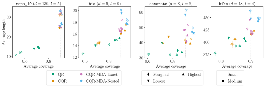
Figure 13: Model is NN. The mask is concatenated in the features. Data is imputed using Iterative Ridge. 100 repetitions are performed, allowing to display the standard error as error bars. The vertical dotted lines represent the target coverage of 90%.

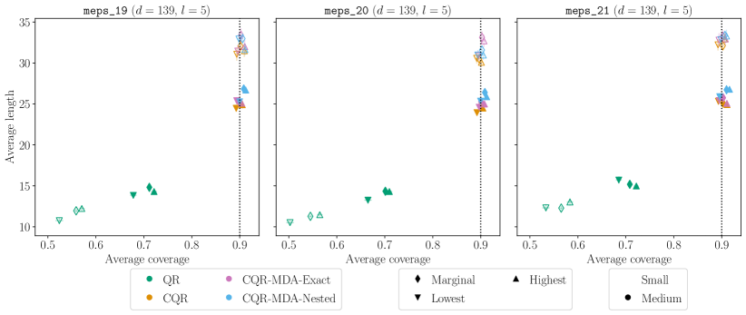
Figure 14: Same caption than Figure 13.

G.5 Real data

Data set description. Sportisse et al., (2020) selected 7 variables to model the level of platelets, after discussion with medical doctors. Thus, we followed their pipeline. Here are the 7 variables used:

• Age: the age of the patient (no missing values);

• Lactate: the conjugate base of lactic acid, upon arrival at the hospital (17.66% missing values);

• Delta_hemo: the difference between the hemoglobin upon arrival at hospital and the one in the ambulance (23.82% missing values);

• VE: binary variable indicating if a Volume Expander was applied in the ambulance. A volume expander is a type of intravenous therapy that has the function of providing volume for the circulatory system (2.46% missing values);

• RBC: a binary index which indicates whether the transfusion of Red Blood Cells Concentrates is performed (0.37% missing values);

• SI: the shock index. It indicates the level of occult shock based on heart rate (HR) and systolic blood pressure (SBP), that is SI = $\frac{\text{HR}}{\text{SBP}}$, upon arrival at hospital (2.09% missing values);

• HR: the heart rate measured upon arrival of hospital (1.62% missing values).

Splitting strategy. To study the coverage conditionally on the masks, we must handle the scarcity of some of them. For each individual in the data set, we make only one prediction, this way avoiding too many repetitions of the same test point when computing the average. We split the data set into 5 folds, and predict on each fold by training the procedure on the 4 others, with 15390 observations for training, and 7694 for calibration.

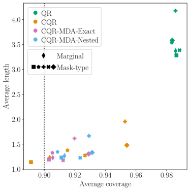
Figure 15: Average coverage and length on the TraumaBase® data when predicting the platelets level. Colors correspond to the methods. Diamond ($\blacklozenge$) corresponds to taking the average among all individuals. Other symbols correspond to computing the average among the individuals having a fixed mask. The vertical dotted line represents the target coverage of 90%. Model is NN. The mask is concatenated to the features. Imputation is Iterative Ridge. Each individual is predicted using 15390 observations for training, and 7694 for calibration.

References

• Angelopoulos and Bates, (2023) Angelopoulos, A. N. and Bates, S. (2023). Conformal Prediction: A Gentle Introduction. Now Foundations and Trends.
• Ayme et al., (2022) Ayme, A., Boyer, C., Dieuleveut, A., and Scornet, E. (2022). Near-optimal rate of consistency for linear models with missing values. In Chaudhuri, K., Jegelka, S., Song, L., Szepesvari, C., Niu, G., and Sabato, S., editors, Proceedings of the 39th International Conference on Machine Learning, volume 162, pages 1211–1243. PMLR.
• (3) Barber, R. F., Candès, E. J., Ramdas, A., and Tibshirani, R. J. (2021a). The limits of distribution-free conditional predictive inference. Information and Inference: A Journal of the IMA, 10(2):455–482.
• (4) Barber, R. F., Candès, E. J., Ramdas, A., and Tibshirani, R. J. (2021b). Predictive inference with the jackknife+. The Annals of Statistics, 49(1):486–507.
• Barber et al., (2022) Barber, R. F., Candès, E. J., Ramdas, A., and Tibshirani, R. J. (2022). Conformal prediction beyond exchangeability.
• Dua and Graff, (2017) Dua, D. and Graff, C. (2017). UCI machine learning repository.
• Eaton, (1983) Eaton, M. L. (1983). Multivariate statistics. John Wiley & Sons, Nashville, TN.
• Gupta et al., (2022) Gupta, C., Kuchibhotla, A. K., and Ramdas, A. (2022). Nested conformal prediction and quantile out-of-bag ensemble methods. Pattern Recognition, 127:108496.
• Izbicki et al., (2020) Izbicki, R., Shimizu, G., and Stern, R. (2020). Flexible distribution-free conditional predictive bands using density estimators. In Chiappa, S. and Calandra, R., editors, Proceedings of the Twenty Third International Conference on Artificial Intelligence and Statistics, volume 108, pages 3068–3077. PMLR.
• Izbicki et al., (2022) Izbicki, R., Shimizu, G., and Stern, R. B. (2022). Cd-split and hpd-split: Efficient conformal regions in high dimensions. Journal of Machine Learning Research, 23(87):1–32.
• Jiang et al., (2022) Jiang, W., Bogdan, M., Josse, J., Majewski, S., Miasojedow, B., Ročková, V., and TraumaBase® Group (2022). Adaptive bayesian slope: Model selection with incomplete data. Journal of Computational and Graphical Statistics, 31(1):113–137.
• Josse et al., (2019) Josse, J., Prost, N., Scornet, E., and Varoquaux, G. (2019). On the consistency of supervised learning with missing values.
• Josse and Reiter, (2018) Josse, J. and Reiter, J. P. (2018). Introduction to the Special Section on Missing Data. Statistical Science, 33(2):139 – 141.
• Kingma and Ba, (2014) Kingma, D. P. and Ba, J. (2014). Adam: A method for stochastic optimization.
• (15) Le Morvan, M., Josse, J., Moreau, T., Scornet, E., and Varoquaux, G. (2020a). Neumiss networks: differentiable programming for supervised learning with missing values. In Larochelle, H., Ranzato, M., Hadsell, R., Balcan, M., and Lin, H., editors, Advances in Neural Information Processing Systems, volume 33, pages 5980–5990. Curran Associates, Inc.
• Le Morvan et al., (2021) Le Morvan, M., Josse, J., Scornet, E., and Varoquaux, G. (2021). What’s a good imputation to predict with missing values? In Ranzato, M., Beygelzimer, A., Dauphin, Y., Liang, P., and Vaughan, J. W., editors, Advances in Neural Information Processing Systems, volume 34, pages 11530–11540. Curran Associates, Inc.
• (17) Le Morvan, M., Prost, N., Josse, J., Scornet, E., and Varoquaux, G. (2020b). Linear predictor on linearly-generated data with missing values: non consistency and solutions. In Chiappa, S. and Calandra, R., editors, Proceedings of the Twenty Third International Conference on Artificial Intelligence and Statistics, volume 108, pages 3165–3174. PMLR.
• Lei et al., (2018) Lei, J., G’Sell, M., Rinaldo, A., Tibshirani, R. J., and Wasserman, L. (2018). Distribution-Free Predictive Inference for Regression. Journal of the American Statistical Association, 113(523):1094–1111.
• Lei and Wasserman, (2014) Lei, J. and Wasserman, L. (2014). Distribution-free prediction bands for non-parametric regression. Journal of the Royal Statistical Society: Series B (Statistical Methodology), 76(1):71–96.
• Lin et al., (2021) Lin, Z., Trivedi, S., and Sun, J. (2021). Locally valid and discriminative prediction intervals for deep learning models. In Ranzato, M., Beygelzimer, A., Dauphin, Y., Liang, P., and Vaughan, J. W., editors, Advances in Neural Information Processing Systems, volume 34, pages 8378–8391. Curran Associates, Inc.
• Little, (2019) Little, R. J. A. (2019). Statistical analysis with missing data, third edition. John Wiley & Sons, Nashville, TN, 3 edition.
• Manokhin, (2022) Manokhin, V. (2022). Awesome conformal prediction.
• Mayer et al., (2019) Mayer, I., Sportisse, A., Josse, J., Tierney, N., and Vialaneix, N. (2019). R-miss-tastic: a unified platform for missing values methods and workflows.
• MEPS, (2016) MEPS (2016). Medical expenditure panel survey. https://meps.ahrq.gov/mepsweb/data_stats/data_overview.jsp.
• Papadopoulos et al., (2002) Papadopoulos, H., Proedrou, K., Vovk, V., and Gammerman, A. (2002). Inductive confidence machines for regression. In Elomaa, T., Mannila, H., and Toivonen, H., editors, Machine Learning: ECML 2002, pages 345–356, Berlin, Heidelberg. Springer Berlin Heidelberg.
• Pedregosa et al., (2011) Pedregosa, F., Varoquaux, G., Gramfort, A., Michel, V., Thirion, B., Grisel, O., Blondel, M., Prettenhofer, P., Weiss, R., Dubourg, V., Vanderplas, J., Passos, A., Cournapeau, D., Brucher, M., Perrot, M., and Duchesnay, E. (2011). Scikit-learn: Machine learning in Python. Journal of Machine Learning Research, 12:2825–2830.
• Romano et al., (2020) Romano, Y., Barber, R. F., Sabatti, C., and Candès, E. (2020). With Malice Toward None: Assessing Uncertainty via Equalized Coverage. Harvard Data Science Review, 2(2).
• Romano et al., (2019) Romano, Y., Patterson, E., and Candès, E. (2019). Conformalized quantile regression. In Wallach, H., Larochelle, H., Beygelzimer, A., d'Alché-Buc, F., Fox, E., and Garnett, R., editors, Advances in Neural Information Processing Systems, volume 32. Curran Associates, Inc.
• Rubin, (1976) Rubin, D. B. (1976). Inference and missing data. Biometrika, 63(3):581–592.
• Sesia and Candès, (2020) Sesia, M. and Candès, E. J. (2020). A comparison of some conformal quantile regression methods. Stat, 9(1):e261.
• Sesia and Romano, (2021) Sesia, M. and Romano, Y. (2021). Conformal prediction using conditional histograms. In Ranzato, M., Beygelzimer, A., Dauphin, Y., Liang, P., and Vaughan, J. W., editors, Advances in Neural Information Processing Systems, volume 34, pages 6304–6315. Curran Associates, Inc.
• Sportisse et al., (2020) Sportisse, A., Boyer, C., Dieuleveut, A., and Josse, J. (2020). Debiasing averaged stochastic gradient descent to handle missing values. In Larochelle, H., Ranzato, M., Hadsell, R., Balcan, M., and Lin, H., editors, Advances in Neural Information Processing Systems, volume 33, pages 12957–12967. Curran Associates, Inc.
• Van Ness et al., (2022) Van Ness, M., Bosschieter, T. M., Halpin-Gregorio, R., and Udell, M. (2022). The missing indicator method: From low to high dimensions.
• Vovk, (2012) Vovk, V. (2012). Conditional validity of inductive conformal predictors. In Hoi, S. C. H. and Buntine, W., editors, Proceedings of the Asian Conference on Machine Learning, volume 25 of Proceedings of Machine Learning Research, pages 475–490, Singapore Management University, Singapore. PMLR.
• Vovk et al., (2005) Vovk, V., Gammerman, A., and Shafer, G. (2005). Algorithmic Learning in a Random World. Springer US.
• Yang, (2015) Yang, M. (2015). Features Handling by Conformal Predictors. PhD thesis, Royal Holloway, University of London.
• Zaffran et al., (2022) Zaffran, M., Féron, O., Goude, Y., Josse, J., and Dieuleveut, A. (2022). Adaptive conformal predictions for time series. In Chaudhuri, K., Jegelka, S., Song, L., Szepesvari, C., Niu, G., and Sabato, S., editors, Proceedings of the 39th International Conference on Machine Learning, volume 162, pages 25834–25866. PMLR.