Go-No go criteria for performing quantum chemistry calculations on quantum computers

Abstract

Quantum chemistry is envisioned as an early and disruptive application for quantum computers. We propose two criteria for evaluating the two leading quantum approaches for this class of problems. The first criterion applies to the Variational Quantum Eigensolver (VQE) algorithm. It sets an upper bound to the level of noise that can be tolerated in quantum hardware as a function of the targetted precision and problem size. We find a crippling effect of noise with an overall scaling of the precision that is generically less favourable than in the corresponding classical algorithms. Indeed, the studied molecule is unrelated to the hardware dynamics, hence to its noise; conversely the hardware noise populates states of arbitrary energy of the studied molecule. The second criterion applies to the Quantum Phase Estimation (QPE) algorithm that is often presented as the go-to replacement of VQE upon availability of (noiseless) fault-tolerant quantum computers. QPE suffers from the orthogonality catastrophe that generically leads to an exponentially small success probability when the size of the problem grows. Our criterion allows one to estimate quantitatively the importance of this phenomenon from the knowledge of the variance of the energy of the input state used in the calculation.

There exists a hierarchy in the applications that have been proposed for quantum computers, from the celebrated Shor algorithm [1] (exponentially faster than its known classical counterparts) to Grover algorithm [2] (up to quadratically faster than its classical counterparts but less specialized, see [3] for the skeptical point of view of one of us) to near-term algorithms such as the Variational Quantum Eigensolver (VQE) [4], which have no a priori parametric advantage over their classical counterparts but might have a practical one. This hierarchy ends with quantum (analog) simulations, where one gives up on the quantum gate model, i.e. on programmability. Going down this hierarchy, one gives up on the advantage provided by the quantum computer in terms of the degree of generality of the applications and arguably the expected provable speedup. In turn, the requirements on the hardware become less drastic, perhaps allowing one to obtain useful results without the need for a fault-tolerant approach [5].

This article focuses on one field that has been put forward as a possible near-term application for quantum computers: quantum chemistry [6, 7]. The leading algorithms are VQE [8, 9, 10, 11] or its fault-tolerant counterpart, the Quantum Phase Estimation (QPE) algorithm [12, 13, 14]. Despite great expectations, it is a very difficult exercise to extrapolate the existing hardware capabilities to estimate whether a quantum advantage will be eventually reached. In this letter, we take a somewhat reverse approach and derive necessary conditions to obtain such an advantage, thereby defining constraints that the hardware must fulfill if an advantage is to be obtained.

A criterion for VQE. We start with an analysis of VQE and the level of quantum noise that it can sustain. The VQE approach is very close in spirit to the classical algorithm of variational Monte-Carlo (VMC) [15]. One constructs a variational anzatz $|\Psi_{V}\rangle=U(\vec{\theta})|0\rangle$ by applying a quantum circuit $U(\vec{\theta})$ to an initial state $|0\rangle$ of a system made of $n$ qubits. The variables $\vec{\theta}$ parametrize the ansatz. In a second step, one estimates the energy $E_{V}=\langle\Psi_{V}|H|\Psi_{V}\rangle$ of the molecule. Here $H$ is the Hamiltonian of the studied molecule, encoded in a form suitable for qubits. The ground state of $H$ is $|\Psi_{0}\rangle$, with a ground state energy $E_{0}$, and one seeks to find $E_{V}\geq E_{0}$ as close to $E_{0}$ as possible. The energy estimation is performed by running the circuit $N_{S}$ times until the statistical uncertainty of the measured quantities $\eta_{S}\propto 1/\sqrt{N_{S}}$ is smaller than the desired precision. Then the parameters $\vec{\theta}$ are updated in order to decrease the variational energy $E_{V}$. The process is repeated until the energy has reached convergence.

A central question for VQE is its accuracy in presence of hardware imperfections such as noise or decoherence. Noise leads to exponentially vanishing gradients [16] (preventing optimization) and quite stringent lower bounds on the lowest achievable variational energy [17]. Important efforts are on-going on noise mitigation [18, 19] but these techniques are generically plagued with an exponential complexity [20, 21, 21, 22, 23]. We measure the effect of the noise on the hardware with the fidelity $F=\langle\Psi_{V}|\rho|\Psi_{V}\rangle$. It expresses how the density matrix $\rho$ of the quantum computer after state preparation differs from the expected one, $|\Psi_{V}\rangle\langle\Psi_{V}|$. A $F<1$ implies that $\rho=F|\Psi_{V}\rangle\langle\Psi_{V}|+(1-F)\rho_{\rm noise}$, where $\rho_{\rm noise}$ is the part of the density matrix that results from decoherence. The resulting energy is given by $E=E_{V}+\Delta E$ with a noise induced error $\Delta E$ defined as

$$\Delta E=(1-F)[E_{\rm noise}-E_{V}],$$ (1)

with $E_{\rm noise}={\rm Tr}(\rho_{\rm noise}H)$. A large corpus of experiments and theory [24], including the seminal ”quantum supremacy” experiment by Google [25], shows that the fidelity decays exponentially with the total number of applied gates $N_{g}$,

$$F\approx e^{-\epsilon N_{g}}$$ (2)

where $\epsilon$ is the average error per gate. In the leading quantum hardware, this error is dominated by the two-qubit gates for which $\epsilon\leq 1\%$.

Suppose that one targets a precision $\eta_{\rm chem}$ in the calculation with $\eta_{\rm chem}\ll E_{\mathrm{noise}}-E_{V}$. It follows that $F$ must be very close to unity. $\Delta E\leq\eta_{\rm chem}$ leads to,

$$\epsilon\leq\frac{\eta_{\rm chem}}{(E_{\rm noise}-E_{0})N_{g}}.$$ (3)

This is our quantitative criterion for using VQE on a given hardware, molecule and ansatz. In addition, $N_{g}$ depends on $\eta_{\rm chem}$: good precision requires complex ansatz with many gates. Note that $\epsilon$ is the effective error that one obtains after one has done ones’ best to decrease the error level, including any error correction scheme and/or error mitigation.

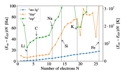
Figure 1: Difference between the energy of the infinite temperature state $E_{\infty}$ and the energy of the ground state, computed within the Hartree-Fock approximation $E_{HF}$, per electron, for the first atoms in the periodic table, from H to Fe for three common basis sets.

We now argue that the energy scale $E_{\mathrm{noise}}-E_{V}$ is generically a large energy scale—of the order of the bare matrix elements of the Hamiltonian, Hartrees or tens of Hartrees—and even generically scales very unfavourably as the square of the number of electrons. Indeed, in general, the target Hamiltonian $H$ is very different from the Hamiltonian that describes the hardware. This is a price gate-based quantum computers pay in exchange for their universality, as opposed to analog quantum simulators. Therefore, the sought-after $|\Psi_{V}\rangle$ is generically a high-energy state of the hardware Hamiltonian. Conversely, hardware noise shares no structure with the studied molecule and it will typically populate eigenstates of $H$ of arbitrary large energies. The above argument—absence of correlations between the hardware spectrum and the studied molecule spectrum—is illustrated in the schematic shown in Fig. 2. For instance, one of the simplest noise channels, the depolarizing noise, maps $\rho\rightarrow(1-\epsilon)\rho+\epsilon I_{d}/2^{n}$, where $I_{d}$ is the identity matrix. It follows that $E_{\rm noise}=E_{\infty}$ for this model, where $E_{\infty}$ is the equilibrium energy of the Hamiltonian $H$ at infinite temperature. Local Pauli errors have the same fixed point [16] and would provide the same energy scale.

The above discussion, combined with the long range nature of the Coulomb interaction, changes the scaling of the noise-induced error. When one puts together $N$ electrons with the $N$ positive charges of the nuclei, the resulting energy scales as $N^{2}$ if the electrons are not allowed to screen the nuclei. The ground-state energy of a molecule scales as $N$ because the electrons properly screen the nuclei. Likewise, any reasonable variational ansatz is extensive. However, the hardware noise is totally unaware of the molecule one wants to study. Hence, it will generically populate the high energy states of $H$. These are the states that have a macroscopic ($\propto N$) electric dipole (classical charging energy of a capacitor). Any noise model that creates a macroscopic electric dipole (i.e. $\rho_{\text{noise}}$ has a finite $N$-independent weight on those states) will lead to a quadratic contribution to the observed energy. For instance energy relaxation favors a single electronic configuration (say all qubits in state zero) that is unlikely to screen the nuclei. Even considering the simple case of the depolarizing noise, there is a macroscopic dipole as soon as one introduces any assymetry in the system. The generic scaling of the noise error is therefore

$$E_{\rm noise}\approx aN+bN^{2},$$ (4)

where the magnitude of the constant $a$ and $b$ will depend on the details of the problem and of the noise model. This is very different from e.g. VMC that does not suffer from this problem (unless a particularly ill-chosen variational ansatz is used). Quantum simulators (aka analog quantum computers) do not generically suffer from this problem either. There, the Hamiltonian of the hardware (and possibly its imperfections) is supposed to match as closely as possible the Hamiltonian that one wants to study. The quadratic scaling of the VQE error is a direct consequence of its added programmability with respect to an analog simulation.

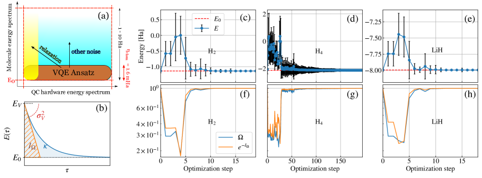
Figure 2: (a) Schematic of the hardware spectrum/studied molecule spectrum duality underlying an important limitation of VQE approaches. The VQE ansatz is close to the ground state of the molecule but is made of arbitrary high energy states of the hardware. Conversely, the hardware noise will populate arbitrary high excited states of the studied molecule.(b) Sketch of the energy $E(\tau)$ versus imaginary time. The area $\kappa$ under the energy curve directly provides the overlap $\Omega=e^{-\kappa}$. We approximate $\kappa$ with the more easily accessible orange-shaded area $I_{\Omega}$. (c), (d) and (e): Energy $E_{V}$ versus optimization step in VQE simulation, the ”error bar” corresponds to the standard deviation $\sigma_{V}$. (f), (g) and (h): Overlap $\Omega$ and $e^{-I_{\Omega}}$ versus optimization step.

We have computed $E_{\rm noise}$ in the case of the depolarising noise for the first $26$ atoms of the periodic table using the PySCF package [26]. Figure 1 shows the energy per electron $(E_{\infty}-E_{\rm HF})/N$ (at this scale $E_{\rm HF}$ is undistinguishable from $E_{0}$) versus $N$. Figure 1 contains three important messages. First, the scale: as soon as one steps away from the minimum STO-3G basis set (which is totally insufficient to achieve chemical accuracy in any setting), the scale of the error is very large, of the order of $10$ Ha. To put it into perspectives, the right axis shows the energies in Kelvins: one quickly arrives at core sun level of temperature. Second, the scale quickly increases when one increases the basis set from single zeta to double and triple. It means that when one improves the basis set to get a better accuracy, the noise induced error actually gets worse. Third, we clearly observe the quadratic contribution $\propto N^{2}$ upon increasing $N$ (see also the supplementary material).

What does the criterion Eq. (3) imply in practice? It is generally accepted that a a quantum chemistry calculation must reach the chemical accuracy ${\eta_{\rm chem}=1{\rm kcal/mol}\ \approx 1.6{\rm mHa}\approx 500K}$ (for energy differences). The energy $E_{\rm noise}$, on the other hand, has a typical value $\geq 1{\rm Ha}$, likely more. For instance for the $H_{2}$ molecule in a minimum basis set of just two orbitals per atom (STO-3G), one gets ${E_{\infty}-E_{0}=1.02{\rm Ha}}$. On the other hand, one needs a variational ansätz expressive enough to reach $\eta_{\rm chem}$, which provides a constraint $N_{g}\geq N_{g}(\eta_{\rm chem},N)$. To be concrete, we consider a recent blind test benchmark on the benzene molecule [27]. Benzene is a non trivial calculation for classical approaches. Yet [27] showcased that a variety of classical techniques arrived at chemical precision using $30$ electrons distributed on $108$ orbitals. Using the UCC ansatz, inspired by the successful coupled cluster approach used in quantum chemistry, would require to include at least single, double and triple excitations (actually quadruple would probably be needed too, again we are being optimistic), which translates into $N_{g}>N^{6}$ gates. One arrives at a noise level $\epsilon\leq 10^{-3}/(30)^{6}$ which translates into $\epsilon\leq 10^{-12}$, that is many orders of magnitude below the best existing quantum hardware.

Another consequence of the noise-induced error is the statistical precision of the calculation. In VQE, one does not measure the energy $E$ directly but rather elements of the one and two-body reduced density matrix, from which one estimates its different subterms separately (kinetic and potential energies). It follows that even if $|\Psi_{V}\rangle$ were exactly equal to the actual ground state (hence the total energy has zero variance), these subterms taken separately would have large standard deviations $\sigma$ ($|\Psi_{V}\rangle$ is not an eigenstate of any of them) of the order of $\sigma\approx 1{\rm Ha}$ or larger. This implies that a large number of shots $N_{S}\gg(\sigma/\eta_{\rm chem})^{2}$ is needed to reach high precision. To this problem, the noise adds a contribution to the variance of the order of $(\Delta E)^{2}$, which can have a drastic impact on the measurement time needed e.g. to implement any noise mitigation scheme. Note that classical methods typically do not suffer from this problem. In a VMC calculation, the statistical error $\eta_{S}$ is given by $\eta_{S}=\sigma_{V}/\sqrt{N_{S}}$ where $\sigma^{2}_{V}=\langle\Psi_{V}|H^{2}|\Psi_{V}\rangle-E_{V}^{2}$ is the variance of the energy of the ansatz. Hence, when the ansatz is properly chosen, it has a low variance (zero if we find the actual ground state of the system) so that one can reach high precision at an affordable $N_{S}$ (in a single shot in the ideal case).

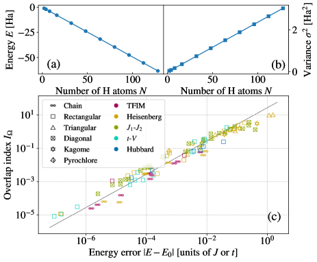
Figure 3: Scaling of the Hartree-Fock energy (a) and the energy variance (b) versus number of atoms in an hydrogen chain. (c): Overlap index $I_{\Omega}$ versus energy error $|E-E_{0}|$ for the variational ansatz of the [28] data set. The dashed line is a linear fit $I_{\Omega}\approx 27.8|E-E_{0}|$.

A criterion for QPE. We now turn to the second criterion, relevant for Quantum Phase Estimation (QPE) algorithm. QPE starts from a guess input state $|\Psi_{V}\rangle$ and projects the state onto the eigenvectors of $e^{-iHt}$, i.e. the eigenvectors of $H$, and extract the corresponding eigenenergy $E_{0}$. QPE is much more demanding than VQE and it is assumed that one is in possession of a hypothetical [29] (noiseless) fault tolerant quantum computer. The probability to obtain the ground state $|\Psi_{0}\rangle$ of $H$ is proportional to the overlap $\Omega=|\langle\Psi_{V}|\Psi_{0}\rangle|^{2}$. A large $\Omega\sim 1$ is crucial for QPE to be useful. In condensed matter, $\Omega$ is believed to decrease exponentially with system size; this is the orthogonality catastrophe [30]. This phenomenon holds even for states that share very similar energies. For instance, the difference of energy per particle between superconducting aluminum and normal-metal aluminium is extremely tiny $\sim(\Delta/E_{F})^{2}\approx 10^{-8}$ ($\Delta$: superconducting gap, $E_{F}$: Fermi energy) yet the two states behave drastically differently. In quantum chemistry, the situation has been studied in less detail: Tubman et al. [31] looked at small molecules with small static correlation (good targets for classical claculations) and concluded that $\Omega$ could be kept to relatively high values, while [32], which looked at more correlated molecules, gave indication of a relatively fast decay of the overlap. We note that calculations on small molecules may be misleadingly optimistic because the variational ansatz may have enough parameters to capture the entire Hilbert space (or a large fraction), in sharp contrast to real situations of interest.

Below we show that the success probability $\Omega$ can actually be estimated in realistic situations where one does not have access to the exact ground state. Let us assume that the initial state $|\Psi_{V}\rangle$ fed to QPE has been obtained using a variational computation like VQE. Then, we use a theorem proved by one of us in [33] to estimate the overlap $\Omega$ of this state with the ground state $|\Psi_{0}\rangle$. Let us consider the wavefunction $|\Psi(\tau)\rangle=\frac{1}{\sqrt{Z}}e^{-H\tau}|\Psi_{V}\rangle$, where the factor $Z=\langle\Psi_{V}|e^{-2H\tau}|\Psi_{V}\rangle$ ensures normalization. This wavefunction appears in various techniques (e.g. Diffusion Monte-Carlo or Green function Monte-Carlo) that project the variational wavefunction onto the groundstate since $\lim_{\tau\rightarrow\infty}|\Psi(\tau)\rangle=|\Psi_{0}\rangle$. A typical output of these methods is the energy $E(\tau)=\langle\Psi(\tau)|H|\Psi(\tau)\rangle$ as a function of $\tau$ as sketched in Fig. 2 (left panel). The success probability of QPE is simply related to the area $\kappa$ under this curve as [33],

$$\Omega=\exp(-\kappa),\mathrm{~{}with~{}}\kappa=\int\limits_{0}^{\infty}d\tau(E(\tau)-E_{0}).$$ (5)

While $\kappa$ is not necessarily easy to compute, a good proxy can be obtained by considering the area $I_{\Omega}$ of the dashed triangle in the left panel of Fig. 2. This area can be calculated from the knowledge of the variational energy $E_{V}=E(\tau=0)$, the energy variance of the variational ansatz $\sigma_{V}^{2}=-\partial_{\tau}E(\tau=0)$ and an estimate (that need not be very accurate) of the ground-state energy $E_{0}$:

$$I_{\Omega}\equiv\frac{(E_{V}-E_{0})^{2}}{2\sigma^{2}}.$$ (6)

We call $I_{\Omega}$ the ”overlap index” of the variational ansatz $|\Psi_{V}\rangle$. $I_{\Omega}$ provides an estimate of $\Omega$,

$$\Omega\approx e^{-I_{\Omega}},$$ (7)

and the associated criterion is naturally $\Omega\sim 1$. This criterion depends on the energy and variance of the ansatz and is totally independent on the imaginary time evolution used for its derivation.

To corroborate the validity of this overlap estimation, we have performed VQE simulations for several molecules, computing both the variational energy and the variance. For these small systems, the exact ground state energy can be calculated as well. This allows to compute the exact overlap $\Omega$ and check that the estimate Eq.(7) holds. On bigger systems, one would rely on estimates such as those currently used in quantum chemistry where one extrapolates from a sequence of increasingly accurate calculations (e.g. CCSD, CCSDT and CCSDTQ calculations). We use the myQLM-fermion package [34], a one-layer UCC ansatz and a minimum basis set (STO-$3$G for H₂ and H₄ molecules; the $6$-$31$G basis and active space selection to reduce the Hilbert space dimension from $22$ to $4$ for LiH). The convergence of the results versus the optimization step are shown on the right panels of Figure 2. Note that the ”error bars” in the upper panels stand for the variance of the variational ansatz. In the lower panels, we observe a very good match between the right and left-hand sides of Eq.(7), which shows that the overlap index is a good proxy for $\Omega$. Our result indicates that the joined calculation of the energy $E_{V}$ and the variance $\sigma_{V}^{2}$ make variational calculations much more valuable. Note that in the H₄ simulation, which uses $8$ qubits in contrast to H₂ and LiH where the number of qubits is only $4$, the convergence is much slower.

We end with a discussion of the scaling that one may expect for $\Omega$. A reasonable variational energy is an extensive quantity $E_{V}\propto N$. Likewise, the variance is also likely to be extensive $\sigma^{2}\propto N$ (this is true if the energy is roughly the sum of local terms). It follows that the overlap index is generically an extensive quantity $I_{\Omega}=\alpha N$, from which one concludes that the overlap decreases exponentially $\Omega\approx e^{-\alpha N}$. This is the orthogonality catastrophe in the context of variational calculations. To illustrate the above statements, the top panels of Figure 3 show the Hartree-Fock energy (left) and variance (right) of hydrogen chains of up to $N=128$ in the STO-$3$G basis set. Both indeed scale linearly with $N$ as advertized. In a slightly different context, a recent work [28] has aggregated a large data set of energies and variances of variational ansatz of various condensed matter systems of various sizes using various methods. The bottom panel of Figure 3 shows $I_{\Omega}$ versus $E_{V}-E_{0}$ for the data set of [28]. We find that $I_{\Omega}$ is well fitted by a linear law $I_{\Omega}=C|E-E_{0}|$, with $C=27.8\pm 0.1$. Since $|E-E_{0}|$ is an extensive quantity, this implies again the exponential decay associated with the orthogonality catastrophe.

To conclude, we have proposed two criteria, one for VQE (noisy hardware) one for QPE (fault tolerant hardware) that are easily accessible and provide necessary conditions for the possibility of doing genuinely relevant chemistry calculations on quantum hardware. Our preliminary estimates imply that this possibility is unlikely with the approaches and technologies that are currently pursued, unless important paradigm shifts take place.

Appendix A Supplementary material

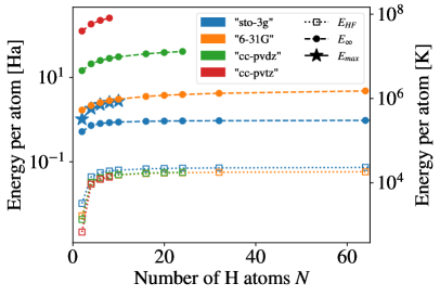
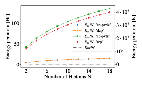
Figure 4: (Left) Hydrogen chain energy scales. Hartree-Fock ground state energy $E_{HF}$ and thermalized energy $E_{\infty}$ per atom, for the ”STO-3G” ($2$ qubits per atom), ”6-31G” ($4$ qubits per atom)  [35], ”cc-pVDZ” ($10$ qubits per atom) and ”cc-pVTZ” basis ($28$ qubits per atom)  [36]. For the ”STO-3G” basis we have plotted the highest excited state energy $E_{max}$ up to $N=10$ (regime where exact diagonalization is possible). For all curves, the zero-offset for energies per atom is $E_{0}(N=2)/2$, where $E_{0}(N=2)$ comes from exact diagonalization of the H₂ Hamiltonian in the ”STO-3G” basis. (Right) Hartree-Fock energy per atom $E_{HF}/N$ and thermalized energy per atom $E_{\infty}/N$ for an asymmetric hydrogen chain where the rightmost-half has AO basis ’sto-3g’ while the leftmost-half has a varying AO basis : ”cc-pvdz”, ”dzp”, ”cc-pvtz”, ”tzp”.

Appendix B Role of the basis set on the noise induced error

Figure 4 shows the energy $E_{\infty}/N$ versus $N$ for a chain of $N$ hydrogen atoms, calculated with the PySCF package [26]. The left panel shows a symmetric case where the same basis set is used on all atoms. The right panel shows an (artificially) assymetric case where the first $N/2$ atoms are treated with a small basis set (STO-3G) while the last $N/2$ atoms are treated with a larger basis set. Also shown on the left panel is the Hartree-Fock energy (empty symbols, almost basis set independent at this scale) and the maximum energy of the Hamiltonian (star, only for STO-3G).

In the simple error model considered here, ($\rho_{\rm noise}\propto I_{\rm d}$), the noise essentially populates the available orbitals in a uniform way. The point we are trying to make is that such a population is likely not to properly screen the nuclei charge, therefore have a dear cost in energy. This is shown in a particularly striking way on the right panel where the assymetry in the basis set leads to the advent of a macroscopic dipole (and the energy increases quadratically with $N$). Even for the case on the left, which is highly symmetric (all atoms play an identical role except fot the two on the edges of the chain), the different orbitals are not identical so that increasing the basis set is very costly in energy. The most important information from these curves is the scale of the noise energy: of the order of $10$ Ha, i.e. four orders of magnitude larger than the targeted accuracy.

References

- Shor [1994] P. Shor, Algorithms for quantum computation: discrete logarithms and factoring, in Proceedings 35th Annual Symposium on Foundations of Computer Science (1994) pp. 124–134.
- Grover [1997] L. K. Grover, Quantum mechanics helps in searching for a needle in a haystack, Phys. Rev. Lett. 79, 325 (1997).
- Stoudenmire and Waintal [2023] E. M. Stoudenmire and X. Waintal, Grover’s algorithm offers no quantum advantage (2023), arXiv:2303.11317 [quant-ph] .
- Peruzzo et al. [2014] A. Peruzzo, J. McClean, P. Shadbolt, M.-H. Yung, X.-Q. Zhou, P. J. Love, A. Aspuru-Guzik, and J. L. O’Brien, A variational eigenvalue solver on a photonic quantum processor, Nature Communications 5, 4213 (2014).
- Ayral et al. [2023a] T. Ayral, P. Besserve, D. Lacroix, and E. A. R. Guzman, Quantum computing with and for many-body physics (2023a), arXiv:2303.04850 [quant-ph] .
- Bauer et al. [2020] B. Bauer, S. Bravyi, M. Motta, and G. K.-L. Chan, Quantum algorithms for quantum chemistry and quantum materials science, Chemical Reviews 120, 12685 (2020), pMID: 33090772, https://doi.org/10.1021/acs.chemrev.9b00829 .
- Tilly et al. [2022] J. Tilly, H. Chen, S. Cao, D. Picozzi, K. Setia, Y. Li, E. Grant, L. Wossnig, I. Rungger, G. H. Booth, and J. Tennyson, The variational quantum eigensolver: A review of methods and best practices, Physics Reports 986, 1 (2022), the Variational Quantum Eigensolver: a review of methods and best practices.
- Kühn et al. [2019] M. Kühn, S. Zanker, P. Deglmann, M. Marthaler, and H. Weiß, Accuracy and resource estimations for quantum chemistry on a near-term quantum computer, Journal of Chemical Theory and Computation 15, 4764 (2019), pMID: 31403781, https://doi.org/10.1021/acs.jctc.9b00236 .
- Elfving et al. [2020] V. E. Elfving, B. W. Broer, M. Webber, J. Gavartin, M. D. Halls, K. P. Lorton, and A. Bochevarov, How will quantum computers provide an industrially relevant computational advantage in quantum chemistry? (2020), arXiv:2009.12472 [quant-ph] .
- Cerezo et al. [2021] M. Cerezo, A. Arrasmith, R. Babbush, S. C. Benjamin, S. Endo, K. Fujii, J. R. McClean, K. Mitarai, X. Yuan, L. Cincio, and P. J. Coles, Variational quantum algorithms, Nature Reviews Physics 3, 625 (2021).
- Gonthier et al. [2022] J. F. Gonthier, M. D. Radin, C. Buda, E. J. Doskocil, C. M. Abuan, and J. Romero, Measurements as a roadblock to near-term practical quantum advantage in chemistry: Resource analysis, Phys. Rev. Res. 4, 033154 (2022).
- Wecker et al. [2015] D. Wecker, M. B. Hastings, and M. Troyer, Progress towards practical quantum variational algorithms, Physical Review A 92, 042303 (2015), arXiv:1507.08969 .
- von Burg et al. [2021] V. von Burg, G. H. Low, T. Häner, D. S. Steiger, M. Reiher, M. Roetteler, and M. Troyer, Quantum computing enhanced computational catalysis, Phys. Rev. Res. 3, 033055 (2021).
- Beverland et al. [2022] M. E. Beverland, P. Murali, M. Troyer, K. M. Svore, T. Hoefler, V. Kliuchnikov, G. H. Low, M. Soeken, A. Sundaram, and A. Vaschillo, Assessing requirements to scale to practical quantum advantage (2022), arXiv:2211.07629 [quant-ph] .
- Ceperley et al. [1977] D. Ceperley, G. V. Chester, and M. H. Kalos, Monte carlo simulation of a many-fermion study, Phys. Rev. B 16, 3081 (1977).
- Wang et al. [2021] S. Wang, E. Fontana, M. Cerezo, K. Sharma, A. Sone, L. Cincio, and P. J. Coles, Noise-induced barren plateaus in variational quantum algorithms, Nature Communications 12, 6961 (2021), arXiv:2007.14384 .
- Stilck França and García-Patrón [2021] D. Stilck França and R. García-Patrón, Limitations of optimization algorithms on noisy quantum devices, Nature Physics 17, 1221 (2021), arXiv:2009.05532 .
- Grimsley et al. [2019] H. R. Grimsley, S. E. Economou, E. Barnes, and N. J. Mayhall, An adaptive variational algorithm for exact molecular simulations on a quantum computer, Nature Communications 10, 3007 (2019), arXiv:arXiv:1812.11173v2 .
- Endo et al. [2021] S. Endo, Z. Cai, S. C. Benjamin, and X. Yuan, Hybrid Quantum-Classical Algorithms and Quantum Error Mitigation, Journal of the Physical Society of Japan 90, 032001 (2021), arXiv:2011.01382v1 .
- Li and Benjamin [2017] Y. Li and S. C. Benjamin, Efficient Variational Quantum Simulator Incorporating Active Error Minimization, Physical Review X 7, 021050 (2017), arXiv:1611.09301 .
- Temme et al. [2017] K. Temme, S. Bravyi, and J. M. Gambetta, Error Mitigation for Short-Depth Quantum Circuits, Physical Review Letters 119, 180509 (2017), arXiv:1612.02058 .
- Endo et al. [2018] S. Endo, S. C. Benjamin, and Y. Li, Practical Quantum Error Mitigation for Near-Future Applications, Physical Review X 8, 031027 (2018), arXiv:1712.09271 .
- Ferracin et al. [2022] S. Ferracin, A. Hashim, J.-L. Ville, R. Naik, A. Carignan-Dugas, H. Qassim, A. Morvan, D. I. Santiago, I. Siddiqi, and J. J. Wallman, Efficiently improving the performance of noisy quantum computers, (2022), arXiv:2201.10672 .
- Ayral et al. [2023b] T. Ayral, T. Louvet, Y. Zhou, C. Lambert, E. M. Stoudenmire, and X. Waintal, Density-matrix renormalization group algorithm for simulating quantum circuits with a finite fidelity, PRX Quantum 4, 020304 (2023b).
- Arute et al. [2020] F. Arute, K. Arya, R. Babbush, D. Bacon, J. C. Bardin, R. Barends, S. Boixo, M. Broughton, B. B. Buckley, D. A. Buell, B. Burkett, N. Bushnell, Y. Chen, Z. Chen, B. Chiaro, R. Collins, W. Courtney, S. Demura, A. Dunsworth, E. Farhi, A. Fowler, B. Foxen, C. Gidney, M. Giustina, R. Graff, S. Habegger, M. P. Harrigan, A. Ho, S. Hong, T. Huang, W. J. Huggins, L. Ioffe, S. V. Isakov, E. Jeffrey, Z. Jiang, C. Jones, D. Kafri, K. Kechedzhi, J. Kelly, S. Kim, P. V. Klimov, A. Korotkov, F. Kostritsa, D. Landhuis, P. Laptev, M. Lindmark, E. Lucero, O. Martin, J. M. Martinis, J. R. McClean, M. McEwen, A. Megrant, X. Mi, M. Mohseni, W. Mruczkiewicz, J. Mutus, O. Naaman, M. Neeley, C. Neill, H. Neven, M. Y. Niu, T. E. O’Brien, E. Ostby, A. Petukhov, H. Putterman, C. Quintana, P. Roushan, N. C. Rubin, D. Sank, K. J. Satzinger, V. Smelyanskiy, D. Strain, K. J. Sung, M. Szalay, T. Y. Takeshita, A. Vainsencher, T. White, N. Wiebe, Z. J. Yao, P. Yeh, and A. Zalcman, Hartree-fock on a superconducting qubit quantum computer, Science 369, 1084 (2020), https://www.science.org/doi/pdf/10.1126/science.abb9811 .
- Sun et al. [2020] Q. Sun, X. Zhang, S. Banerjee, P. Bao, M. Barbry, N. S. Blunt, N. A. Bogdanov, G. H. Booth, J. Chen, Z.-H. Cui, J. J. Eriksen, Y. Gao, S. Guo, J. Hermann, M. R. Hermes, K. Koh, P. Koval, S. Lehtola, Z. Li, J. Liu, N. Mardirossian, J. D. McClain, M. Motta, B. Mussard, H. Q. Pham, A. Pulkin, W. Purwanto, P. J. Robinson, E. Ronca, E. R. Sayfutyarova, M. Scheurer, H. F. Schurkus, J. E. T. Smith, C. Sun, S.-N. Sun, S. Upadhyay, L. K. Wagner, X. Wang, A. White, J. D. Whitfield, M. J. Williamson, S. Wouters, J. Yang, J. M. Yu, T. Zhu, T. C. Berkelbach, S. Sharma, A. Y. Sokolov, and G. K.-L. Chan, Recent developments in the PySCF program package, The Journal of Chemical Physics 153, 10.1063/5.0006074 (2020), 024109, https://pubs.aip.org/aip/jcp/article-pdf/doi/10.1063/5.0006074/16722275/024109_1_online.pdf .
- Eriksen et al. [2020] J. J. Eriksen, T. A. Anderson, J. E. Deustua, K. Ghanem, D. Hait, M. R. Hoffmann, S. Lee, D. S. Levine, I. Magoulas, J. Shen, N. M. Tubman, K. B. Whaley, E. Xu, Y. Yao, N. Zhang, A. Alavi, G. K.-L. Chan, M. Head-Gordon, W. Liu, P. Piecuch, S. Sharma, S. L. Ten-no, C. J. Umrigar, and J. Gauss, The ground state electronic energy of benzene, The Journal of Physical Chemistry Letters 11, 8922 (2020), pMID: 33022176, https://doi.org/10.1021/acs.jpclett.0c02621 .
- Wu et al. [2023] D. Wu, R. Rossi, F. Vicentini, N. Astrakhantsev, F. Becca, X. Cao, J. Carrasquilla, F. Ferrari, A. Georges, M. Hibat-Allah, M. Imada, A. M. Läuchli, G. Mazzola, A. Mezzacapo, A. Millis, J. R. Moreno, T. Neupert, Y. Nomura, J. Nys, O. Parcollet, R. Pohle, I. Romero, M. Schmid, J. M. Silvester, S. Sorella, L. F. Tocchio, L. Wang, S. R. White, A. Wietek, Q. Yang, Y. Yang, S. Zhang, and G. Carleo, Variational benchmarks for quantum many-body problems (2023).
- Waintal [2019] X. Waintal, What determines the ultimate precision of a quantum computer, Phys. Rev. A 99, 042318 (2019).
- Anderson [1967] P. W. Anderson, Infrared catastrophe in fermi gases with local scattering potentials, Phys. Rev. Lett. 18, 1049 (1967).
- Tubman et al. [2018] N. M. Tubman, C. Mejuto-Zaera, J. M. Epstein, D. Hait, D. S. Levine, W. Huggins, Z. Jiang, J. R. McClean, R. Babbush, M. Head-Gordon, and K. B. Whaley, Postponing the orthogonality catastrophe: efficient state preparation for electronic structure simulations on quantum devices (2018), arXiv:1809.05523 [quant-ph] .
- Lee et al. [2022] S. Lee, J. Lee, H. Zhai, Y. Tong, A. M. Dalzell, A. Kumar, P. Helms, J. Gray, Z.-H. Cui, W. Liu, M. Kastoryano, R. Babbush, J. Preskill, D. R. Reichman, E. T. Campbell, E. F. Valeev, L. Lin, and G. K.-L. Chan, Is there evidence for exponential quantum advantage in quantum chemistry? (2022).
- Mora and Waintal [2007] C. Mora and X. Waintal, Variational wave functions and their overlap with the ground state, Physical review letters 99, 030403 (2007).
- Haidar et al. [2022] M. Haidar, M. J. Rančić, T. Ayral, Y. Maday, and J.-P. Piquemal, Open source variational quantum eigensolver extension of the quantum learning machine (qlm) for quantum chemistry (2022).
- Ditchfield et al. [1971] R. Ditchfield, W. J. Hehre, and J. A. Pople, Self‐consistent molecular‐orbital methods. ix. an extended gaussian‐type basis for molecular‐orbital studies of organic molecules, The Journal of Chemical Physics 54, 724 (1971), https://doi.org/10.1063/1.1674902 .
- Dunning [1989] T. H. Dunning, Gaussian basis sets for use in correlated molecular calculations. i. the atoms boron through neon and hydrogen, The Journal of Chemical Physics 90, 1007 (1989), https://doi.org/10.1063/1.456153 .