Permutation Decision Trees

Abstract

Decision Tree is a well understood Machine Learning model that is based on minimizing impurities in the internal nodes. The most common impurity measures are Shannon entropy and Gini impurity. These impurity measures are insensitive to the order of training data and hence the final tree obtained is invariant to any permutation of the data. This leads to a serious limitation in modeling data instances that have order dependencies. In this work, we propose the use of Effort-To-Compress (ETC) - a complexity measure, for the first time, as an impurity measure. Unlike Shannon entropy and Gini impurity, structural impurity based on ETC is able to capture order dependencies in the data, thus obtaining potentially different decision trees for different permutations of the same data instances (Permutation Decision Trees). We then introduce the notion of Permutation Bagging achieved using permutation decision trees without the need for random feature selection and sub-sampling. We compare the performance of the proposed permutation bagged decision trees with Random Forests. Our model does not assume that the data instances are independent and identically distributed. Potential applications include scenarios where a temporal order present in the data instances is to be respected.

1 Introduction

The assumptions in Machine Learning (ML) models play a crucial role not just in appropriate applicability but also in interpretability, reproducibility, and generalizability. One common assumption is that the dataset is independent and identically distributed (i.i.d). However, in reality, this assumption rarely holds true, as human learning often involves connecting new information with what was previously observed. Psychological theories such as Primacy and Recency Effects [1], Serial Position Effect, and Frame Effect suggest that the order in which data is presented can significantly impact decision-making processes. In this work, we have devised a learning algorithm that exhibits sensitivity to the order in which data is presented. This unique characteristic imparts our proposed model with decision boundaries or decision functions that rely on the specific arrangement of training data.

In our research, we introduce the novel use of ‘Effort-To-Compress’ (ETC) – a compression-complexity measure – as an impurity function for Decision Trees, marking the first instance of its application in Machine Learning. ETC effectively measures the effort required for lossless compression of an object through a predetermined lossless compression algorithm [2]. ETC was initially introduced in [3] as a measure of complexity for timeseries analysis, aiming to overcome the severe limitations of entropy-based complexity measures. It is worth noting that the concept of complexity lacks a singular, universally accepted definition. In [2], complexity was explored from different perspectives, including the effort-to-describe (Shannon entropy, Lempel-Ziv complexity), effort-to-compress (ETC complexity), and degree-of-order (Subsymmetry). The same paper highlighted the superior performance of ETC in distinguishing between periodic and chaotic timeseries. Moreover, ETC has played a pivotal role in the development of an interventional causality testing method known as Compression-Complexity-Causality (CCC) [4]. CCC and allied approaches based on compression-complexity have been rigorously tested in several practical applications for causal discovery and inference [5, 6, 7, 8]. ETC has demonstrated robust, reliable and superior performance over infotheoretic approaches when applied to short and noisy time series data (including stochastic and/or chaotic ones), leading to its utilization in diverse fields such as investigating cardiovascular dynamics [9], conducting cognitive research [10], and analysis of muscial compositions [11].

In this research, we present a new application of ETC in the field of Machine Learning, offering a fresh perspective on its ability to capture structural impurity. Leveraging this insight, we introduce a decision tree classifier that maximizes the ETC gain (analogous to information gain in conventional decision trees). It is crucial to highlight that Shannon entropy and Gini impurity fall short in capturing structural impurity, resulting in an impurity measure that disregards the data’s underlying structure (in terms of order). The utilization of ETC as an impurity measure provides the distinct advantage of generating different decision trees for various permutations of data instances. Consequently, this approach frees us from the need to adhere strictly to the i.i.d. assumption commonly employed in Machine Learning. In fact, ETC itself makes no such assumption of the timeseries for characterizing its complexity. Thus, by simply permuting data instances, we can develop a Permutation Decision Forest.

The paper is organized as follows: Section 2 introduces the Proposed Method, Section 3 presents the Experiments and Results, Section 4 describes Model interpretability, Section 5 discusses the Limitations of our research, and Section 6 provides the concluding remarks and outlines the future work.

2 Proposed Method

In this section, we establish the concept of structural impurity and subsequently present an illustrative example to aid in comprehending the functionality of ETC.

Definition: Structural impurity for a sequence $S=s_{0},s_{1},\ldots,s_{n}$, where $s_{i}\in\{0,1,\ldots,K\}$, and $K\in\mathbf{Z^{+}}$ is the extent of irregularity in the sequence $S$.

The above definition is purposefully generic in its use of the term irregularity and one could use several specific measures of irregularity. We suggest a specific measure, namely ‘Effort-To-Compress’ or ETC for measuring the extent of irregularity in the input sequence $S$ and thus inturn serving as a measure of structual impurity.

We will now illustrate how ETC serves as a measure of structural impurity. The formal definition of ETC is the effort required for the lossless compression of an object using a predefined lossless compression algorithm. The specific algorithm employed to compute ETC is known as Non-sequential Recursive Pair Substitution (NSRPS). NSRPS was initially proposed by Ebeling [12] in 1980 and has since undergone improvements [13], ultimately proving to be an optimal choice [14]. Notably, NSRPS has been extensively utilized to estimate the entropy of written English [15]. The algorithm is briefly discussed below: Let’s consider the sequence $S=00011$ to demonstrate the iterative steps of the algorithm. In each iteration, we identify the pair of symbols with the highest frequency and replace all non-overlapping instances of that pair with a new symbol. In the case of sequence $S$, the pair with the maximum occurrence is $00$. We substitute all occurrences of $00$ with a new symbol, let’s say $2$, resulting in the transformed sequence $2011$. We continue applying the algorithm iteratively. The sequence $2011$ is further modified to become $311$, where the pair $20$ is replaced by $3$. Then, the sequence $311$ is transformed into $41$ by replacing $31$ with $4$. Finally, the sequence $41$ is substituted with $5$. At this point, the algorithm terminates as the stopping criterion is achieved when the sequence becomes homogeneous. ETC, as defined in [3], is equal to the count of the number of iterations needed for the NSRPS algorithm to attain a homogeneous sequence when applied iteratively on the input sequence (as described above).

We consider the structural impurity (computed using ETC) of the following binary sequences and compare it with Shannon entropy and Gini impurity measures.

Table 1: Comparison of Structural impurity computed using ETC with Shannon entropy, and Gini impurity for various binary sequences.

Sequence ID	Sequence	Structural Impurity (ETC)	Entropy	Gini Impurity
A	111111	0	0	0
B	121212	1	1	0.5
C	222111	5	1	0.5
D	122112	4	1	0.5
E	211122	5	1	0.5

Referring to Table 1, we observe that for sequence A, the ETC, Shannon Entropy, and Gini impurity all have a value of zero. This outcome arises from the fact that the sequence is homogeneous, devoid of any impurity. Conversely, for sequences B, C, D, and E, the Shannon entropy and Gini impurity remain constant, whereas ETC varies based on the particular structural characteristics of each sequence. Thus, ETC is able to capture the structural impurity in sequences, better than both Shannon entropy and Gini impurity measures. Having shown that the ETC captures the structural impurity of a sequence, we now define ETC Gain. ETC gain is the reduction in ETC caused by partioning the data instances according to a particular attribute of the dataset. Consider the decision tree structure provided in Figure 1.

Figure 1: Decision Tree structure with a parent node and two child node (Left Child and Right Child).

The ETC Gain between the chosen parent attribute ($P$) of the tree and the class labels ($S$) is defined as follows:

$$ETC~{}Gain(S,P)=ETC(S)-\displaystyle\sum\limits_{V\in Values(P)}\frac{|S_{V}|}{|S|}\cdot ETC(S_{V}),$$ (1)

where $V$ in equation 1 is the possible values of the chosen parent attribute $P$, $S_{V}\subset S$, and $S_{V}$ consists of labels corresponding to the chosen parent attribute $P$ taking the value $V$, $|S|$ represents the cardinality of the set $S$. The formula for ETC Gain, as given in equation 1, bears resemblance to information gain. The key distinction lies in the use of ETC as a measure of structural impurity instead of Shannon entropy in the calculation. We now provide the different steps in the Permutation Decision Tree (PDT) algorithm.

1. Step 1: Choose an attribute to be the root node and create branches corresponding to each possible value of the attribute.

2. Step 2: Evaluate the quality of the split using ETC gain.

3. Step 3: Repeat Step 1 and Step 2 for all other attributes, recording the quality of split based on ETC gain.

4. Step 4: Select the partial tree with the highest ETC gain as a measure of quality of split.

5. Step 5: Iterate Steps 1 to 4 for each child node of the selected partial tree.

6. Step 6: If all instances at a node share the same classification (homogeneous class), stop developing that part of the tree.

3 Experiments and Results

To showcase the effectiveness of the proposed structural impurity measure (computed using ETC) in capturing the underlying structural dependencies within the data and subsequently generating distinct decision trees for different permutations of input data, we utilize the following illustrative toy example.

Table 2: Toy example dataset to demonstrate permuted decision trees generated with a novel structural impurity measure (computed using ETC). The toy example considered is a binary classification problem (class-1, class-2) with two features $f_{0}$, $f_{1}$ and $14$ data instance. The rows represents different training data instances.

Serial No.	$f_{0}$	$f_{1}$	label
1	1	1	2
2	1	2	2
3	1	3	2
4	2	1	2
5	2	2	2
6	2	3	2
7	4	1	2
8	4	2	2
9	4	3	1
10	4	4	1
11	5	1	1
12	5	2	1
13	5	3	1
14	5	4	1

The visual representation of the toy example provided in Table 2 is represented in Figure 2.

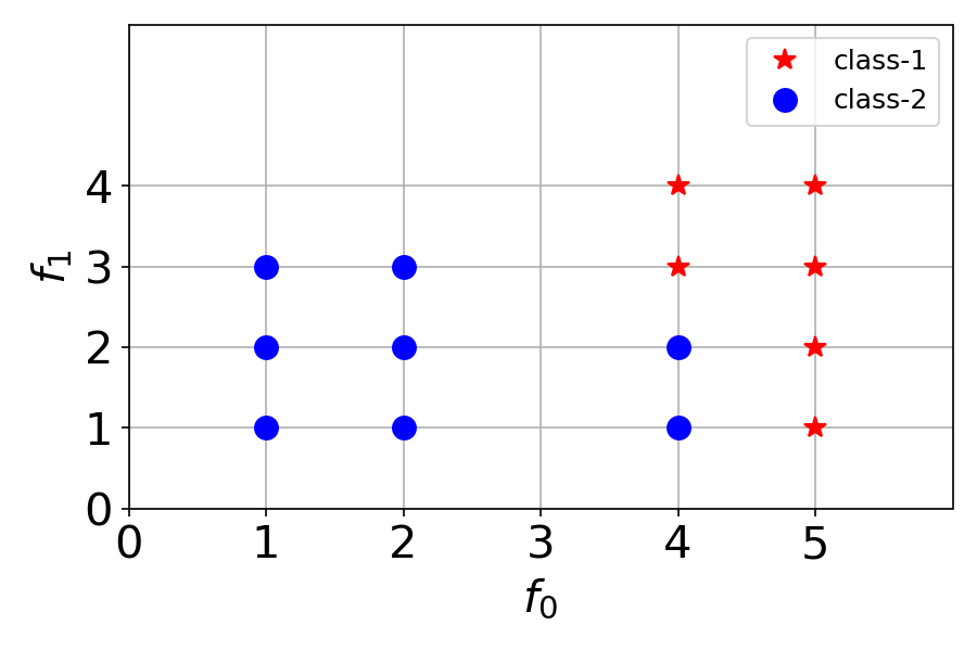
Figure 2: A visual representation of the toy example provided in Table 2.

We consider the following permutations of the dataset. For each of the below permutations, we obtain distinct decision trees using the proposed structural impurity measure (computed using ETC).

• Permutation A: 1, 2, 3, 4, 5, 6, 7, 8, 9, 10, 11, 12, 13, 14. Figure 3 represents the corresponding decision tree.

  Figure 3: Decision tree using the proposed structural impurity (computed using ETC) for Permutation A.

• Permutation B: 14, 3, 10, 12, 2, 4, 5, 11, 9, 8, 7, 1, 6, 13. Figure 4 represents the corresponding decision tree.

  Figure 4: Decision tree using the proposed structural impurity (computed using ETC) for Permutation B.

• Permutation C: 13, 11, 8, 12, 7, 6, 4, 14, 10, 5, 2, 3, 1, 9. Figure 5 represents the corresponding decision tree.

  Figure 5: Decision tree using the proposed structural impurity (computed using ETC) for Permutation C.

• Permutation D: 3, 2, 13, 10, 11, 1, 4, 7, 6, 9, 8, 14, 5, 12. Figure 6 represents the corresponding decision tree.

  Figure 6: Decision tree using the proposed structural impurity (computed using ETC) for Permutation D.

• Permutation E: 10, 12, 1, 2, 13, 14, 8, 11, 4, 7, 9, 6, 5, 3. Figure 7 represents the corresponding decision tree.

  Figure 7: Decision tree using the proposed structural impurity (computed using ETC) for Permutation E.

The variability in decision trees obtained from different permutations of data instances (Figures 3, 4, 5, 6,and  7) can be attributed to the ETC measure’s ability to capture the structural impurity of labels, which was not possible for both Shannon entropy and Gini impurity. Table  3 highlights the sensitivity of ETC to permutation, contrasting with the insensitivity of Shannon entropy and Gini impurity towards data instance permutations. In the given toy example, there are six class-1 data instances and eight class-2 data instances. Since Shannon entropy and Gini impurity are probability-based methods, they remain invariant to label permutation. This sensitivity of ETC to the structural pattern of the label motivates us to develop a bagging algorithm namely Permutation Decision Forest.

Table 3: Comparison between Shannon Entropy, Gini Impurity and Structural Impurity (computed using ETC) for the 5 chosen permutations of the data instances of the toy example. Notice the insensitivity of both Shannon entropy and Gini impurity in capturing the changes in the structure of the labels. ETC is able to capture even small changes in structure/ order/ pattern.

Label Impurity	Shannon Entropy (bits)	Gini Impurity	Structural Impurity (ETC)
Permutation A	0.985	0.490	7
Permutation B	0.985	0.490	8
Permutation C	0.985	0.490	9
Permutation D	0.985	0.490	9
Permutation E	0.985	0.490	8

3.1 Temporal vs. Spatial Ordering in Decision Making

In the toy example (Table 2), the data instances were represented spatially (refer to Figure 2). However, it is also possible to imagine the data instances to be events in time. This has significant bearing on the decision making process.

Imagine that there is an outbreak of a new virus (like COVID-19) and data instances (rows of Table 2) correspond to chronological admission of patients to a testing facility. The decision to be taken is to quarantine (if virus is present) or not quarantine the patient (if no virus present). Let $f_{0}$ represent the severity (including diversity) of symptoms of the incoming patient and $f_{1}$ represent the value obtained by a molecular test performed on a bio-sample (for eg., blood sample) taken from the patient. The labels ‘$1$’ and ‘$2$’ correspond to the presence of virus (POSITIVE) and absence of the virus (NEGATIVE) respectively. Consequently, the patient with POSITIVE label is quarantined. It is also the case that determining the severity (and diversity) of symptoms is relatively straightforward as it involves a thorough examination by the attending physician. On the other hand, performing the molecular test on the patient’s blood sample involves considerable cost and time, and not to mention the discomfort the patient is subjected to. The decision making process needs to factor in all these additional constraints.

Now, the permutations A-E of the data correspond to different realities in which the events happen over time. Even though all the $14$ patients with exactly the same severity of symptoms and molecular test value occur (we assume that the molecular test is done on all the patients for the purposes of medical records), the order in which they arrive is different in each of these realities. Consequently, the decision tree obtained by our method is going to be different in each reality which is intuitive and reasonable. Conventional DT with information gain or Gini impurity would make no distinction between these realities and yield the same DT in each reality. However, this would not be ideal as we shall show.

To illustrate the contrasting decision trees obtained by the ETC based impurity measure, consider the trees obtained for permutation B and permutation D. We have re-drawn them below to better aid the comparison (refer to Figure 8 and Figure 9). Both decision trees fit the same data (up to a permutation) and hence have identical performance metrics. However, the former needs molecular testing of all $14$ patients whereas the later needs the testing to be done on only $4$ patients. The argument to be made here is that in the reality encountered by permutation D, the incoming patients arrive in a particular order where it becomes necessary to decide to perform the molecular testing on all of them. Whereas, in the alternate reality corresponding to permutation B, the patients arrive in such an order that the decision to test first on severity of symptoms is the correct one. This has a huge impact on future events – in Figure 8, each and every patient in the future will also be subjected to the molecular testing whereas not in the case of Figure 9. Thus, decision making strictly depends on the chronological ordering of events - as is the case in real life.

Figure 8: Decision tree using the proposed structural impurity (computed using ETC) for Permutation B. This decision tree requires the molecular testing of all $14$ patients (and any future patient as well).

Figure 9: Decision tree using the proposed structural impurity (computed using ETC) for Permutation D. This decision tree requires the molecular testing of only $4$ patients. Not all future patients will be subjected to the molecular testing.

4 Performance comparison of Permutation Decision Tree and Decision Tree

We compare the performance evaluation of the PDT with DT. In our experiments, for PDT and DT, we first split the data randomly into training (80%) and testing (20%). This random seed used for splitting is kept the same for both PDT and DT. After this, we do threefold crossvalidation using time-series spliting  to find the best max_depth of PDT and DT. The max_depth was varied from 1 to 150 with a stepsize of 10. Using the best hyperparameter, we test the efficacy of DT and PDT on the test set. The performance comparison of Decision Tree and Permutation Decision Tree is provided in Table 4.

Table 4: Performance comparison of Decision Tree and Permutation Decision Tree for various publicly available datasets.

Datasets	Decision Tree			Permutation Decision Tree
	Crossvalidation Results (Macro F1-score)	Max_depth	Test Data Results (Macro F1-score)	Crossvalidation Results (Macro F1-score)	Max_depth	Test Data Results (Macro F1-score)
Iris	0.915	11	0.966	0.935	1	0.966
Breast Cancer Wisconsin	0.935	11	0.761	0.899	11	0.893
Haberman’s Survival	0.612	1	0.595	0.637	11	0.527
Ionosphere	0.861	11	0.862	0.820	11	0.862
Seeds	0.903	11	0.834	0.848	1	0.741
Wine	0.856	11	0.879	0892	11	0.878

From Table 4, we could find that PDT gives comparable performance with DT for Iris, Ionosphere, Wine datasets. PDT (macro F1-score = 0.893) outperforms DT (macro F1-score = 0.761) in Breast Cancer Wisconsin dataset, whereas DT (macro F1-score = 0.834) outperforms PDT (macro F1-score = 0.741) in Seeds dataset.

4.1 Permutation Decision Forest

Permutation decision forest distinguishes itself from Random Forest by eliminating the need for random subsampling of data and feature selection in order to generate distinct decision trees. Instead, permutation decision forest achieves tree diversity through permutation of the data instances. Since different permutations of the data instances have potentially different structural impurities, we are guaranteed to have a diversity of decision trees by using a large number of permutations. Figure 10 illustrates the operational flow of the proposed permutation decision forest algorithm.

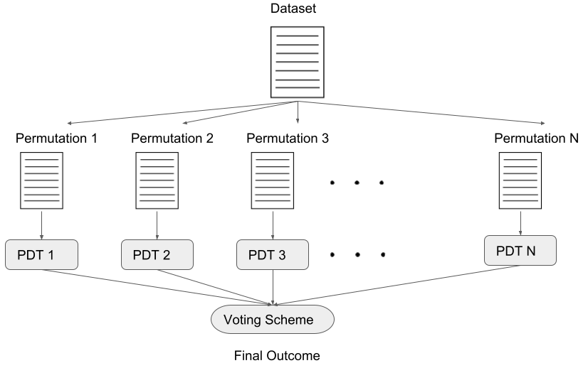
Figure 10: Permutation Decision Forest. The input dataset is subjected to a large number of permutations resulting in different ordering of the data instances. Each such permutation is then used to create a specific permutation decision tree using the structural impurity measure (computed using ETC) as the splitting criteria (ETC gain). The results from each permutation decision tree are then fed into a majority voting scheme to determine the final predicted label.

Figure 10 showcases the workflow of the proposed Permutation Decision Forest algorithm, illustrating its functioning. Consisting of individual permutation decision trees, each tree operates on a permuted dataset to construct a classification model, collectively forming a strong classifier. The outcomes of the permutation decision trees are then fed into a majority voting scheme, where the final predicted label is determined by majority votes. Notably, the key distinction between the Permutation Decision Forest and Random Forest lies in their approaches to obtaining distinct decision trees. While Random Forest relies on random subsampling and feature selection, Permutation Decision Forest achieves diversity through permutation of the input data. This is guaranteed by the sensitivity of the structural impurity measure (computed using ETC) to changes in the structure/order/pattern of labels for different permutations of the data instances. Random forest algorithm does not have this benefit since the impurity measure used (Shannon entropy or Gini impurity) is not sensitive to permutations of the data-instances and would yield only one single tree for every permutation. Hence, diversity of trees is impossible to obtain using Random forest algorithm via permutations. This distinction is significant as random feature selection in Random Forest may result in information loss, which is avoided in Permutation Decision Forest.

4.2 Performance comparison between Random Forest and Permutation Decision Forest

We evaluate the performance of the proposed method with the following datasets: Iris [16], Breast Cancer Wisconsin [17], Haberman’s Survival [18], Ionosphere [19], Seeds [20], Wine [21]. For all datasets, we allocate 80% of the data for training and reserve the remaining 20% for testing. For Random Forest, we performed five fold crossvalidation for n_estimators $=[1,10,100,1000,10000]$ and max_depth ranging from 1 to 11. Due to computational constraints, hyperparameter tuning was not performed for Permutation Decision Forest. The hyperparameters used for Permutation Decision Forest and Random Forest are provided in Table 5.

Table 5 provides a comparison of the hyperparameters used and the test data performance as measured by macro F1-score.

Table 5: Performance comparison of Permutation Decision Forest with Random Forest for various publicly available datasets.

Dataset	Random Forest			Permutation Decision Forest
	F1-score	n_estimators	max_depth	F1-score	n_estimators	max_depth
Iris	1.000	100	3	0.931	31	10
Breast Cancer Wisconsin	0.918	1000	9	0.893	5	10
Haberman’s Survival	0.560	1	3	0.621	5	10
Ionosphere	0.980	1000	4	0.910	5	5
Seeds	0.877	100	5	0.877	11	10
Wine	0.960	10	4	0.943	5	10

In our experimental evaluations, we observed that the proposed method surpasses Random Forest (F1-score = 0.56) solely for the Haberman’s survival dataset (F1-score = 0.621). However, for the Seeds dataset, the permutation decision forest yields comparable performance to Random Forest (F1-score = 0.877). In the remaining cases, Random Forest outperforms the proposed method. Notwithstanding these somewhat underwhelming results which are purely quantitative in nature, we now move to the important qualitative notions of interpretability, explainability, generalizability and causality considerations in the next section. The strength of our methods will become evident in these discussions.

5 Model vs. domain interpretability, temporal generalizability and causal decision learning

The procedure of bagging that is employed in Random forests is problematic from the perspective of interpreatability or explainability. Leaving out some of the features and a random sampling of data instances is bound to result in biased decision trees. Even though the final classification performance of Random forest may be good, the use of biased trees due to random sampling and feature subsampling leads to a loss of interpretability and reliability in the decision making process. It should be noted that leaving out a particular feature or a data instance for constructing a decision tree (as is the case in Random forest algorithm) is completely unjustified from the point of view of the application domain. It is an arbitrary adhoc step that has no valid justification from an explainability/interpretability point of view. Consider the scenario where the left out data instance is an anomaly or a rare event with physical or engineering significance. For example, the data instance that has been removed pertains to a system overload event or a fault event in the monitoring of a power system. In a cyber security scenario, the left out data instance could be an adversarial attack (which is sparse and very rare event). The objective or the goal of the learning task in these applications is in fact to model such rare/extreme/anomalous events in order to understand and garner insights, in which case, the decision tree used to arrive at the final classification rule in Random forest is completely non-intuitive.

In Permutation Decision forest, every permutation of the data instance corresponds to an ‘alternate’ reality (a counterfactual?!) where that particular order of the data instances are presented to the algorithm to result in a specific set of decisions made subsequently by the classifier. Two different permutations of the same data could mean/signify entirely two different realities or states of the world. If each data instance corresponds to a specific time, then a different ordering corresponds to a different temporal sequence of events - which is clearly a very different reality to one that produce the training data. Random forest has no way of capturing these counterfactual realities. Thanks to the sensitivity of the structural impurity measure to data ordering, Permutation Decision forest is able to efficiently capture this via different decision making rules. In effect, what Permutation Decision forest is learning is a generalized set of decision rules that are invariant (under all permutations) to temporal re-ordering. This is a form of generalization which is missing in Random forest. We could call this type of generalization – a form of temporal generalization that respects counterfactual realities. Thus, Permutation Decision forest is a pre-cursor to a causality [22] informed decision tree algorithm. Future research work will focus on making these causal underpinnings more explicit and pronounced with suitable enhancements to upgrade Permutation Decision forest to a full-blow causal reasoning/ causal decision learning algorithm.

5.1 Trade Off between Model Interpretability and Domain Interpretability

Decision trees utilizing traditional impurity measures like Shannon entropy and Gini impurity assist in interpreting the model. However, this does not ensure a comparable level of interpretability for a domain expert. This is because the notion of information is strictly statistical in nature and the underlying assumption of data instances being i.i.d. is a very limiting one. Furthermore, the fact that the ordering of data instances is completely ignored in conventional decision trees is a major limitation, especially in applications where a specific ordering could pertain to an arrow of time that is necessary for a proper interpretation of events. There could also be cases where it is crucial to present multiple decision trees to the domain expert (pertaining to different permutation/ordering of data instances), allowing them to select the most meaningful decision tree, keeping the context of the specific application at hand. This trade-off between model interpretability and domain interpretability is essential to consider, which is simply not possible in conventional decision trees and random forest algorithms. We anticipate that this permutation decision tree will facilitate human involvement in making expert decisions, ensuring a human-in-the-loop approach.

6 Limitations and the way forward

The current framework demonstrates that the proposed method, permutation decision forest, achieves slightly lower classification scores compared to random forest. We acknowledge this limitation and aim to address it in our future work by conducting thorough testing on diverse publicly available datasets (and also by combining permutation bagging with conventional bagging techniques). It is important to note that permutation decision trees offer an advantage when dealing with datasets that possess a temporal order in the generation of data instances. In such scenarios, permutation decision trees can effectively capture the specific temporal ordering within the dataset. We have illustrated the same using a toy example. In our future endeavors, we intend to incorporate and explore this aspect more comprehensively. Also, as alluded to in the previous section, the possibility of building a causal decision learning algorithm based on learning from counterfactual reasoning using structural impurity will be investigated.

7 Conclusions

In this research, we present a unique approach that unveils the interpretation of the Effort-to-Compress (ETC) complexity measure as an impurity measure capable of capturing structural impurity in timeseries data. ETC is proven to be more effective in capturing structural irregularities in the data better than first order entropy based measures. Building upon this insight, we incorporate ETC into Decision Trees, resulting in the introduction of the innovative Permutation Decision Tree. By leveraging permutation, Permutation Decision Tree facilitates the generation of distinct decision trees for varying permutations of data instances. Inspired by this, we further develop a bagging method known as Permutation Decision Forest, which harnesses the power of permutation decision trees which overcomes the limitations of random forest imposed by random subsampling and fearture selection. Particularly, nowhere do we assume that data instances are independent and identically distributed. Moving forward, we are committed to subjecting our proposed method to rigorous testing using diverse publicly available datasets. Additionally, we envision the application of our method in detecting adversarial attacks.

References

- [1] Jamie Murphy, Charles Hofacker, and Richard Mizerski. Primacy and recency effects on clicking behavior. Journal of computer-mediated communication, 11(2):522–535, 2006.
- [2] Nithin Nagaraj and Karthi Balasubramanian. Three perspectives on complexity: entropy, compression, subsymmetry. The European Physical Journal Special Topics, 226:3251–3272, 2017.
- [3] Nithin Nagaraj, Karthi Balasubramanian, and Sutirth Dey. A new complexity measure for time series analysis and classification. The European Physical Journal Special Topics, 222(3-4):847–860, 2013.
- [4] Aditi Kathpalia and Nithin Nagaraj. Data-based intervention approach for complexity-causality measure. PeerJ Computer Science, 5:e196, 2019.
- [5] SY Pranay and Nithin Nagaraj. Causal discovery using compression-complexity measures. Journal of Biomedical Informatics, 117:103724, 2021.
- [6] Vikram Ramanan, Nikhil A Baraiya, and SR Chakravarthy. Detection and identification of nature of mutual synchronization for low-and high-frequency non-premixed syngas combustion dynamics. Nonlinear Dynamics, 108(2):1357–1370, 2022.
- [7] Aditi Kathpalia, Pouya Manshour, and Milan Paluš. Compression complexity with ordinal patterns for robust causal inference in irregularly sampled time series. Scientific Reports, 12(1):1–14, 2022.
- [8] Harikrishnan NB, Aditi Kathpalia, and Nithin Nagaraj. Causality preserving chaotic transformation and classification using neurochaos learning. Advances in Neural Information Processing Systems, 35:2046–2058, 2022.
- [9] Karthi Balasubramanian, K Harikumar, Nithin Nagaraj, and Sandipan Pati. Vagus nerve stimulation modulates complexity of heart rate variability differently during sleep and wakefulness. Annals of Indian Academy of Neurology, 20(4):403, 2017.
- [10] Vasilios K Kimiskidis, Christos Koutlis, Alkiviadis Tsimpiris, Reetta Kälviäinen, Philippe Ryvlin, and Dimitris Kugiumtzis. Transcranial magnetic stimulation combined with eeg reveals covert states of elevated excitability in the human epileptic brain. International journal of neural systems, 25(05):1550018, 2015.
- [11] Abhishek Nandekar, Preeth Khona, MB Rajani, Anindya Sinha, and Nithin Nagaraj. Causal analysis of carnatic music compositions. In 2021 IEEE International Conference on Electronics, Computing and Communication Technologies (CONECCT), pages 1–6. IEEE, 2021.
- [12] Werner Ebeling and Miguel A Jiménez-Montaño. On grammars, complexity, and information measures of biological macromolecules. Mathematical Biosciences, 52(1-2):53–71, 1980.
- [13] Miguel A Jiménez-Montaño, Werner Ebeling, Thomas Pohl, and Paul E Rapp. Entropy and complexity of finite sequences as fluctuating quantities. Biosystems, 64(1-3):23–32, 2002.
- [14] Dario Benedetto, Emanuele Caglioti, and Davide Gabrielli. Non-sequential recursive pair substitution: some rigorous results. Journal of Statistical Mechanics: Theory and Experiment, 2006(09):P09011, 2006.
- [15] Peter Grassberger. Data compression and entropy estimates by non-sequential recursive pair substitution. arXiv preprint physics/0207023, 2002.
- [16] R. A. Fisher. The use of multiple measurements in taxonomic problems. Annals of Eugenics, 7(2):179–188, 1936.
- [17] W Nick Street, William H Wolberg, and Olvi L Mangasarian. Nuclear feature extraction for breast tumor diagnosis. In Biomedical image processing and biomedical visualization, volume 1905, pages 861–870. SPIE, 1993.
- [18] Shelby J Haberman. The analysis of residuals in cross-classified tables. Biometrics, pages 205–220, 1973.
- [19] Vincent G Sigillito, Simon P Wing, Larrie V Hutton, and Kile B Baker. Classification of radar returns from the ionosphere using neural networks. Johns Hopkins APL Technical Digest, 10(3):262–266, 1989.
- [20] Dheeru Dua and Casey Graff. UCI machine learning repository, 2017.
- [21] Michele Forina, Riccardo Leardi, Armanino C, and Sergio Lanteri. PARVUS: An Extendable Package of Programs for Data Exploration. 01 1998.
- [22] Judea Pearl and Dana Mackenzie. The book of why: the new science of cause and effect. Basic books, 2018.