Stochastic Population Update Can Provably Be Helpful
in Multi-Objective Evolutionary Algorithms^†

Abstract

Evolutionary algorithms (EAs) have been widely and successfully applied to solve multi-objective optimization problems, due to their nature of population-based search. Population update, a key component in multi-objective EAs (MOEAs), is usually performed in a greedy, deterministic manner. That is, the next-generation population is formed by selecting the best solutions from the current population and newly-generated solutions (irrespective of the selection criteria used such as Pareto dominance, crowdedness and indicators). In this paper, we question this practice. We analytically present that stochastic population update can be beneficial for the search of MOEAs. Specifically, we prove that the expected running time of two well-established MOEAs, SMS-EMOA and NSGA-II, for solving two bi-objective problems, OneJumpZeroJump and bi-objective RealRoyalRoad, can be exponentially decreased if replacing its deterministic population update mechanism by a stochastic one. Empirical studies also verify the effectiveness of the proposed population update method. This work is an attempt to challenge a common practice in the design of existing MOEAs. Its positive results, which might hold more generally, should encourage the exploration of developing new MOEAs in the area.

[]Corresponding author

1 Introduction

Multi-objective optimization refers to an optimization scenario that there are more than one objective to be considered at the same time. They are very common in real-world applications. For example, in neural architecture search lu2019nsga , researchers and practitioners may try to find an architecture with higher accuracy and lower complexity; in industrial manufacturing pahl1996engineering , production managers would like to devise a product with higher quality and lower cost; in financial investment markowitz1952portfolio , investment managers are keen to build a portfolio with higher return and lower risk. Since the objectives of a multi-objective optimization problem (MOP) are usually conflicting, there does not exist a single optimal solution, but instead a set of solutions which represent different trade-offs between these objectives, called Pareto optimal solutions. The images of all Pareto optimal solutions of a MOP in the objective space are called the Pareto front. In multi-objective optimization, the goal of an optimizer is to find a good approximation of the Pareto front.

Evolutionary algorithms (EAs) back:96 ; eiben2015introduction are a large class of randomized heuristic optimization algorithms inspired by natural evolution. They maintain a set of solutions, i.e., a population, and iteratively improve it by generating new solutions and replacing inferior ones. Due to the population-based nature, EAs are well-suited to solving MOPs, and have been widely used in various real-world scenarios  deb2001book ; qian19el ; coello2007evolutionary ; zhou2011survey including scheduling lee2007multi , aerodynamic design obayashi1998transonic , bioinformatics shin2005dna , etc. In fact, there have been many well-known, widely used multi-objective EAs (MOEAs), with the representations of non-dominated sorting genetic algorithm II (NSGA-II) deb-tec02-nsgaii , $\mathcal{S}$ metric selection evolutionary multi-objective optimization algorithm (SMS-EMOA) beume2007sms , strength Pareto evolutionary algorithm 2 (SPEA2) zitzler2001spea2 , and multi-objective evolutionary algorithm based on decomposition (MOEA/D) zhang2007moea .

In MOEAs, two key components are solution generation and population update. Solution generation is concerned with parent selection and reproduction (e.g., crossover and mutation), while population update (also called environmental selection or population maintenance) is concerned with maintaining a population which represents diverse high-quality solutions found, served as a pool for generating even better solutions. In the evolutionary multi-objective optimization area, the research focus is mainly on population update. That is, when designing an MOEA, attention is predominantly paid on how to update the population by newly-generated solutions so that a set of well-distributed high-quality solutions are preserved. With this aim, many selection criteria emerge, such as non-dominated sorting goldberg1989genetic , crowding distance deb-tec02-nsgaii , scalarizing functions zhang2007moea and quality indicators zitzler2004indicator .

A prominent feature in population update of MOEAs is its deterministic manner. That is, the next-generation population is formed by always selecting the first population-size ranked solutions out of the collections of the current population and newly-generated solutions. This practice may be based on the commonly-held belief that a population formed by the best solutions found so far has a higher chance to generate even better solutions.

In this paper, we challenge this belief. We analytically show that introducing randomness into the population update procedure may be beneficial for the search. Specifically, we consider two well-established MOEAs, SMS-EMOA and NSGA-II, which adopt the $(\mu+1)$ and $(\mu+\mu)$ elitist population update mode, respectively. That is, SMS-EMOA selects the $\mu$ best solutions from the collections of the current population and the newly generated offspring solution to form the next population; NSGA-II selects the $\mu$ best solutions from the collections of the current population and the $\mu$ newly-generated offspring solutions. Note that selecting the best solutions means removing the worst solution(s), i.e., SMS-EMOA removes the only one worst solution, while NSGA-II removes the $\mu$ worst solutions.

We consider a simple stochastic population update method, which first randomly selects a subset from the collections of the current population and the offspring solutions(s), and then removes the worst solution(s) from the subset. That is, the remaining solutions in the selected subset and those unselected solutions form the next population. We theoretically show that this simple modification enables SMS-EMOA and NSGA-II to work significantly better on OneJumpZeroJump  and bi-objective RealRoyalRoad, two bi-objective optimization problems commonly used in theoretical analyses of MOEAs doerr2021ojzj ; doerr2023ojzj ; doerr2023lower ; doerr2023crossover ; dang2023crossover . Specifically, we analyze the expected running time of SMS-EMOA and NSGA-II, under the original deterministic population update mechanism and under the stochastic population update mechanism, on OneJumpZeroJump and bi-objective RealRoyalRoad. The results are summarized in Table 1. As can be seen in the table, the stochastic population update can bring an exponential acceleration. For example, for SMS-EMOA solving OneJumpZeroJump, when $k=\Omega(n)\wedge k=n/2-\Omega(n)$ and $2(n-2k+4)\leq\mu=poly(n)$, using the stochastic population update can bring an acceleration of $\Omega(2^{k/4}/\mu^{2})$, i.e., exponential acceleration, where $n$ denotes the problem size, $k$ ($2\leq k<n/2$) denotes the parameter of OneJumpZeroJump, $\mu$ denotes the population size, and $poly(n)$ denotes any polynomial of $n$. Intuitively, the reason for this occurrence is that by introducing randomness into the population update procedure, the evolutionary search has a chance to go along inferior regions which are close to Pareto optimal regions, thereby making the search easier, compared to bigger jump needed to reach the optimal regions in the original deterministic, greedy procedure. Experiments are also conducted to verify our theoretical results.

Table 1: The expected number of generations of SMS-EMOA and NSGA-II for solving the OneJumpZeroJump and bi-objective RealRoyalRoad problems when the original deterministic or the stochastic population update procedure is used, where $n$ denotes the problem size, $k$ ($2\leq k<n/2$) denotes the parameter of OneJumpZeroJump, and $\mu$ denotes the population size. Note that the equations in the square brackets denote the conditions of the theorems, and $poly(n)$ denotes any polynomial of $n$.

		OneJumpZeroJump	Bi-objective RealRoyalRoad
SMS- EMOA	Deterministic	$O(\mu n^{k})$	$O(\mu n^{n/5-2})$
		[Thm 3.1, $\mu\geq n-2k+3$]	[Thm 3.7, $\mu\geq 2n/5+1$]
		$\Omega(n^{k})$	$\Omega(n^{n/5-1})$
		[Thm 3.3, $n-2k=\Omega(n)\wedge\mu=poly(n)$]	[Thm 3.9, $\mu=poly(n)$]
	Stochastic	$O(\mu^{2}n^{k}/2^{k/4})$	$O(\mu^{2}n^{n/5}/2^{n/20})$
		[Thm 3.4, $\mu\geq 2(n-2k+4)$]	[Thm 3.10, $\mu\geq 2(2n/5+2)$]
NSGA-II	Deterministic	$\Omega(n^{k}/\mu)$	$\Omega(n^{n/5-1}/\mu)$
		[Thm 4.1, $n-2k=\Omega(n)\wedge\mu=poly(n)$]	[Thm 4.4, $\mu=poly(n)$]
	Stochastic	$O(k(n/2)^{k})$	$O(n(20e^{2})^{n/5})$
		[Thm 4.2, $\mu\geq 8(n-2k+3)$]	[Thm 4.5, $\mu\geq 8(2n/5+1)$]

Over the last decade, there is an increasing interest for the theory community to study MOEAs. Primitive theoretical work mainly focuses on analyzing the expected running time of GSEMO Giel03 /SEMO LaumannsTEC04 , a simple MOEA which employs the bit-wise/one-bit mutation operator to generate an offspring solution in each iteration and keeps the non-dominated solutions generated-so-far in the population. GSEMO and SEMO have been analytically employed to solve a variety of multi-objective synthetic and combinatorial optimization problems Giel03 ; laumanns-nc04-knapsack ; LaumannsTEC04 ; Neumann07 ; Horoba09 ; Giel10 ; Neumann10 ; doerr2013lower ; Qian13 ; bian2018tools . In addition, the expected running time of SEMO in the presence of noise is analyzed dinot2023runtime . Moreover, based on GSEMO and SEMO, the effectiveness of some components and methods in evolutionary search, e.g., greedy parent selection LaumannsTEC04 , diversity-based parent selection plateaus10 ; osuna2020diversity , fairness-based parent selection LaumannsTEC04 ; friedrich2011illustration , fast mutation and stagnation detection doerr2021ojzj , crossover Qian13 , and selection hyper-heuristics qian-ppsn16-hyper , has also been studied.

Recently, researchers have started attempts to analyze practical MOEAs. The expected running time of $(\mu+1)$ SIBEA, i.e., a simple MOEA using the hypervolume indicator to update the population, was analyzed on several synthetic problems brockhoff2008analyzing ; nguyen2015sibea ; doerr2016runtime , which benefits the theoretical understanding of indicator-based MOEAs. Later, people have started to consider well-established algorithms in the evolutionary multi-objective optimization area. Huang et al. huang2021runtime considered MOEA/D, and examined the effectiveness of different decomposition methods by comparing the running time for solving many-objective synthetic problems. Zheng et al. zheng2021first analyzed the expected running time of NSGA-II for the first time, by considering the bi-objective OneMinMax and LeadingOnesTrailingZeroes problems. Later on, Zheng and Doerr zheng2022current considered a modified crowding distance method, which updates the crowding distance of solutions once the solution with the smallest crowding distance is removed, and proved that the modified method can approximate the Pareto front better than the original crowding distance method in NSGA-II. Bian and Qian bian2022better proposed a new parent selection method, stochastic tournament selection (i.e., $k$ tournament selection where $k$ is uniformly sampled at random), to replace the binary tournament selection of NSGA-II, and proved that the method can decrease the expected running time asymptotically. The effectiveness of the fast mutation doerr2023ojzj and crossover doerr2023crossover ; dang2023crossover operators in NSGA-II have also been analyzed. Other results include the analysis of NSGA-II solving diverse problems such as the bi-objective multimodal problem OneJumpZeroJump doerr2023ojzj , the many-objective problem $m$OneMinMax zheng2023manyobj , the bi-objective minimum spanning tree problem cerf2023first , and the noisy LeadingOnesTrailingZeroes problem dang2023analysing , as well as an investigation into the lower bounds of NSGA-II solving OneMinMax and OneJumpZeroJump doerr2023lower . Furthermore, Wietheger and Doerr wietheger23nsgaiii proved that NSGA-III deb2014nsgaiii can be better than NSGA-II when solving the tri-objective problem $3$OneMinMax. Very recently, Lu et al. lu2024imoea analyzed interactive MOEAs (iMOEAs) and identified situations where iMOEAs may work or fail.

Our running time analysis about SMS-EMOA contributes to the theoretical understanding of another major type of MOEAs, i.e., combining non-dominated sorting and quality indicators to update the population, for the first time. More importantly, in contrast to the above studies, a distinctive point of the proposed work is that we aim to challenge a common belief that existing practical MOEAs are built upon - always being in favor of better solutions in the population update procedure. We show that introducing randomness that essentially gives a chance for inferior solutions to survive can benefit the search significantly in some cases. Similar observation also exists in some parallel empirical work li2023nonelitist ; li2023moeas in the evolutionary multi-objective optimization area. In li2023moeas , well-established MOEAs (e.g., NSGA-II and SMS-EMOA) have been found to stagnate in a different area at a time, indicating that always preserving the best solutions can make the search easy to get stuck in a “random” local optimum. In li2023nonelitist , a simple non-elitist MOEA, which is of the stochastic population update nature (i.e., worse solutions can survive in the evolutionary process), has been found to outperform NSGA-II on popular practical problems like multi-objective knapsack zitzler1999multiobjective and multi-objective NK-landscape aguirre2004insights .

In this paper, we significantly extend our preliminary work bian23stochastic which analyzed SMS-EMOA on the OneJumpZeroJump problem. In this paper, we add another popular algorithm NSGA-II which has a rather different population update mechanism (in terms of both selection criteria and evolutionary mode). Moreover, we add another multi-objective optimization problem, bi-objective RealRoyalRoad, which is of different features from OneJumpZeroJump. It is worth noting that very recently, Zheng and Doerr zheng2024sms have extended SMS-EMOA to solving a many-objective problem, $m$OneJumpZeroJump, showing that the stochastic population update can bring an acceleration of $\Omega(2^{k/2}/((2n/m-2k+3)^{m/2}k^{1/2}))$ as well, where $n$ is the problem size, $k$ ($k\leq n/m$) is the parameter of $m$OneJumpZeroJump, and $m$ is the number of objectives. Particularly, when $m$ is not too large (e.g., a constant), and $k$ is large (e.g., $\Theta(n)$), the acceleration is exponential. This positive result in many-objective optimization further confirms our finding that introducing randomness into the population update procedure can be beneficial for the search of MOEAs.

The rest of this paper is organized as follows. Section 2 introduces some preliminaries. The running time of SMS-EMOA and NSGA-II using the deterministic and stochastic population update is analyzed in Sections 3 and 4, respectively. Section 5 presents the experimental results. Finally, Section 6 concludes the paper.

2 Preliminaries

In this section, we first introduce multi-objective optimization. Then, we introduce the analyzed algorithms, SMS-EMOA and NSGA-II, and the stochastic population update method. Finally, we present the OneJumpZeroJump and bi-objective RealRoyalRoad problems studied in this paper.

2.1 Multi-objective Optimization

Multi-objective optimization aims to optimize two or more objective functions simultaneously, as shown in Definition 2.1. Note that in this paper, we consider maximization (minimization can be defined similarly), and pseudo-Boolean functions, i.e., the solution space $\mathcal{X}=\{0,1\}^{n}$. The objectives are usually conflicting, thus there is no canonical complete order in the solution space $\mathcal{X}$, and we use the domination relationship in Definition 2.2 to compare solutions. A solution is Pareto optimal if there is no other solution in $\mathcal{X}$ that dominates it, and the set of objective vectors of all the Pareto optimal solutions constitutes the Pareto front. The goal of multi-objective optimization is to find the Pareto front or its good approximation.

Definition 2.1 (Multi-objective Optimization).

Given a feasible solution space $\mathcal{X}$ and objective functions $f_{1},f_{2},\ldots,f_{m}$, multi-objective optimization can be formulated as

$$\max_{\bm{x}\in\mathcal{X}}\bm{f}(\bm{x})=\max_{\bm{x}\in\mathcal{X}}\big{(}f_{1}(\bm{x}),f_{2}(\bm{x}),...,f_{m}(\bm{x})\big{)}.$$

Definition 2.2 (Domination).

Let $\bm{f}=(f_{1},f_{2},\ldots,f_{m}):\mathcal{X}\rightarrow\mathbb{R}^{m}$ be the objective vector. For two solutions $\bm{x}$ and $\bm{y}\in\mathcal{X}$:

• $\bm{x}$ weakly dominates $\bm{y}$ (denoted as $\bm{x}\succeq\bm{y}$) if for any $1\leq i\leq m,f_{i}(\bm{x})\geq f_{i}(\bm{y})$;

• $\bm{x}$ dominates $\bm{y}$ (denoted as $\bm{x}\succ\bm{y}$) if $\bm{x}\succeq\bm{y}$ and $f_{i}(\bm{x})>f_{i}(\bm{y})$ for some $i$;

• $\bm{x}$ and $\bm{y}$ are incomparable if neither $\bm{x}\succeq\bm{y}$ nor $\bm{y}\succeq\bm{x}$.

2.2 SMS-EMOA and NSGA-II Algorithms

The SMS-EMOA algorithm beume2007sms , as presented in Algorithm 1, is a popular MOEA, which employs non-dominated sorting and hypervolume indicator to evaluate the quality of a solution and update the population. SMS-EMOA starts from an initial population of $\mu$ solutions (line 1). In each generation, it randomly selects a solution from the current population (line 3), and applies bit-wise mutation to generate an offspring solution (line 4). Then, the worst solution in the union of the current population $P$ and the newly generated solution is removed (line 5), by using the Population Update of SMS-EMOA subroutine as presented in Algorithm 2. The subroutine first partitions a set $Q$ of solutions (where $Q=P\cup\{\bm{x}^{\prime}\}$ in Algorithm 1) into non-dominated sets $R_{1},R_{2},\ldots,R_{v}$ (line 1), where $R_{1}$ contains all the non-dominated solutions in $Q$, and $R_{i}$ ($i\geq 2$) contains all the non-dominated solutions in $Q\setminus\cup_{j=1}^{i-1}R_{j}$. Then, one solution $\bm{z}\in R_{v}$ that minimizes

$$\Delta_{\bm{r}}(\bm{x},R_{v}):=HV_{\bm{r}}(R_{v})-HV_{\bm{r}}(R_{v}\setminus\{\bm{x}\})$$

is removed (lines 2–3), where $HV_{\bm{r}}(R_{v})=\Lambda\big{(}\cup_{\bm{x}\in R_{v}}\{\bm{f}^{\prime}\in\mathbb{R}^{m}\mid\forall 1\leq i\leq m:r_{i}\leq f^{\prime}_{i}\leq f_{i}(\bm{x})\}\big{)}$ denotes the hypervolume of $R_{v}$ with respect to a reference point $\bm{r}\in\mathbb{R}^{m}$ (satisfying $\forall 1\leq i\leq m,r_{i}\leq\min_{\bm{x}\in\mathcal{X}}f_{i}(\bm{x})$), and $\Lambda$ denotes the Lebesgue measure. The hypervolume of a solution set measures the volume of the objective space between the reference point and the objective vectors of the solution set, and a larger hypervolume value implies a better approximation ability with regards to both convergence and diversity. This implies that the solution with the least value of $\Delta$ in the last non-dominated set $R_{v}$ is regarded as the worst solution and thus removed.

Algorithm 1 SMS-EMOA beume2007sms

Input: objective functions $f_{1},f_{2}\ldots,f_{m}$, population size $\mu$
Output: $\mu$ solutions from $\{0,1\}^{n}$

1:  $P\leftarrow\mu$ solutions uniformly and randomly selected from $\{0,\!1\}^{\!n}$ with replacement;

2:  while criterion is not met do

3:     select a solution $\bm{x}$ from $P$ uniformly at random;

4:     generate $\bm{x}^{\prime}$ by flipping each bit of $\bm{x}$ independently with probability $1/n$;

5:     $P\leftarrow$ Population Update of SMS-EMOA $(P\cup\{\bm{x}^{\prime}\})$

6:  end while

7:  return  $P$

Algorithm 2 Population Update of SMS-EMOA ($Q$) 

Input: a set $Q$ of solutions, and a reference point $\bm{r}\in\mathbb{R}^{m}$
Output: $|Q|-1$ solutions from $Q$

1:  partition $Q$ into non-dominated sets $R_{1},R_{2},\ldots,R_{v}$;

2:  let $\bm{z}=\arg\min_{\bm{x}\in R_{v}}\Delta_{\bm{r}}(\bm{x},R_{v})$;

3:  return  $Q\setminus\{\bm{z}\}$

Algorithm 3 NSGA-II Algorithm deb-tec02-nsgaii

Input: objective functions $f_{1},f_{2}\ldots,f_{m}$, population size $\mu$
Output: $\mu$ solutions from $\{0,1\}^{n}$

1:  $P\leftarrow\mu$ solutions uniformly and randomly selected from $\{0,\!1\}^{\!n}$;

2:  while criterion is not met do

3:     $P^{\prime}=\emptyset$;

4:     for each solution $\bm{x}$ in $P$ do

5:        generate $\bm{x}^{\prime}$ by flipping each bit of $\bm{x}$ independently with probability $1/n$;

6:        add $\bm{x}^{\prime}$ into $P^{\prime}$

7:     end for

8:     $P\leftarrow$ Population Update of NSGA-II $(P\cup P^{\prime})$

9:  end while

10:  return  $P$

Algorithm 4 Population Update of NSGA-II ($Q$) 

Input: a set $Q$ of solutions
Output: $|Q|/2$ solutions from $Q$

1:  partition $Q$ into non-dominated sets $R_{1},R_{2},\ldots,R_{v}$;

2:  let $O=\emptyset$, $i=1$;

3:  while $|O\cup R_{i}|<|Q|/2$ do

4:     $O=O\cup R_{i}$, $i=i+1$

5:  end while

6:  assign each solution in $R_{i}$ with a crowding distance;

7:  add $|Q|/2-|O|$ solutions in $R_{i}$ with the largest crowding distance into $O$;

8:  return  $O$

The NSGA-II algorithm deb-tec02-nsgaii , as presented in Algorithm 3, is probably the most popular MOEA, which incorporates two substantial features, i.e., non-dominated sorting and crowding distance. NSGA-II starts from an initial population of $\mu$ random solutions (line 1). In each generation, it applies bit-wise mutation on each of the solution in the population to generate $\mu$ offspring solutions (lines 3–7). Then, the $\mu$ worst solutions in the union of the current population $P$ and the offspring population are removed (line 8), by using the Population Update of NSGA-II subroutine as presented in Algorithm 4. Similar to Algorithm 2, the subroutine also partitions the set $Q$ of solutions (note that $|Q|=2\mu$) into non-dominated sets $R_{1},R_{2},\ldots,R_{v}$ (line 1). Then, the solutions in $R_{1},R_{2},\ldots,R_{v}$ are added into the next population (lines 3–5), until the population size exceeds $\mu$. For the critical set $R_{i}$ whose inclusion makes the population size larger than $\mu$, the crowding distance is computed for each of the contained solutions (line 6). Crowding distance reflects the level of crowdedness of a solution in the population. For each objective $f_{j}$, $1\leq j\leq m$, the solutions in $R_{i}$ are sorted according to their objective values, and the crowding distance of the solution in the first and the last place is set to infinite. For the solution in the inner part of the sorted list, its crowding distance is set to the difference of the objective values of its neighbouring solutions, divided by $\max_{\bm{x}\in R_{i}}f_{j}(\bm{x})-\min_{\bm{x}\in R_{i}}f_{j}(\bm{x})$, i.e., the maximum difference of the objective values. The complete crowding distance of a solution is the sum of the crowding distance with respect to each objective. Finally, the solutions in $R_{i}$ with the largest crowding distance are selected to fill the remaining population slots (line 7).

Algorithm 5 Stochastic Population Update of SMS-EMOA ($Q$) 

Input: a set $Q$ of solutions, and a reference point $\bm{r}\in\mathbb{R}^{m}$
Output: $|Q|-1$ solutions from $Q$

1:  $Q^{\prime}\leftarrow\lfloor|Q|/2\rfloor$ solutions uniformly and randomly selected from $Q$ without replacement;

2:  partition $Q^{\prime}$ into non-dominated sets $R_{1},R_{2},\ldots,R_{v}$;

3:  let $\bm{z}=\arg\min_{\bm{x}\in R_{v}}\Delta_{\bm{r}}(\bm{x},R_{v})$;

4:  return  $Q\setminus\{\bm{z}\}$

Algorithm 6 Stochastic Population Update of NSGA-II ($Q$) 

Input: a set $Q$ of solutions
Output: $|Q|/2$ solutions from $Q$

1:  $Q^{\prime}\leftarrow\lfloor 3|Q|/4\rfloor$ solutions uniformly and randomly selected from $Q$ without replacement;

2:  partition $Q^{\prime}$ into non-dominated sets $R_{1},R_{2},\ldots,R_{v}$;

3:  let $O=\emptyset$, $i=1$;

4:  while $|O\cup R_{i}|<\lfloor|Q|/4\rfloor$ do

5:     $O=O\cup R_{i}$, $i=i+1$

6:  end while

7:  assign each solution in $R_{i}$ with a crowding distance;

8:  add $\lfloor|Q|/4\rfloor-|O|$ solutions in $R_{i}$ with the largest crowding distance into $O$

9:  return  $Q\setminus(Q^{\prime}\setminus O)$

2.3 Stochastic Population Update

Well-established MOEAs only considered deterministic population update methods. For example, SMS-EMOA always prefers a dominating solution or a solution with a better indicator value, and NSGA-II always prefers a dominating solution or a solution with a larger crowding distance. However, these methods may be too greedy, thus hindering the performance of MOEAs. In this paper, we introduce randomness into the population update procedure of SMS-EMOA and NSGA-II. For SMS-EMOA, Stochastic Population Update of SMS-EMOA as presented in Algorithm 5 is used to replace the original Population Update of SMS-EMOA procedure in line 5 of Algorithm 1; for NSGA-II, Stochastic Population Update of NSGA-II as presented in Algorithm 6 is used to replace the original Population Update of NSGA-II procedure in line 8 of Algorithm 3. The stochastic methods are similar to the original deterministic population update methods, except that the removed solution (solutions) is (are) selected from a subset $Q^{\prime}$ of $Q$, instead of from the entire set $Q$. Specifically, in Algorithm 5, $\lfloor|Q|/2\rfloor$ (i.e., $\lfloor(\mu+1)/2\rfloor$) solutions are first selected from $Q$ uniformly and randomly without replacement (line 1), and then one solution in the set of the selected solutions is removed according to non-dominated sorting and hypervolume (lines 2–4). In Algorithm 6, $\lfloor 3|Q|/4\rfloor$ (i.e., $\lfloor 3\mu/2\rfloor$) solutions are first selected from $Q$ uniformly and randomly without replacement (line 1), and then $|Q|/2$ (i.e., $\mu$) solutions in the set of the selected solutions are removed according to non-dominated sorting and crowding distance (lines 2–9). Note that the size of the selected subset is set to $\lfloor|Q|/2\rfloor$ for SMS-EMOA and $\lfloor 3|Q|/4\rfloor$ for NSGA-II in this paper. However, other values can also be used in practical applications.

2.4 OneJumpZeroJump and Bi-objective RealRoyalRoad Problems

The OneJumpZeroJump problem is a multi-objective counterpart of the Jump problem, a classical single-objective pseudo-Boolean benchmark problem in EAs’ theoretical analyses doerr-20-book . The goal of the Jump problem is to maximize the number of 1-bits of a solution, except for a valley around $1^{n}$ (the solution with all 1-bits) where the number of 1-bits should be minimized. Formally, it aims to find an $n$-bits binary string which maximizes

$$g(\bm{x})=\begin{cases}k+|\bm{x}|_{1},&\text{if }|\bm{x}|_{1}\leq n-k\text{ or }\bm{x}=1^{n},\\ n-|\bm{x}|_{1},&\text{else},\end{cases}$$

where $k\in[2..n-1]$, and $|\bm{x}|_{1}$ denotes the number of $1$-bits in $\bm{x}$. Note that we use $[a..b]$ (where $a,b\in\mathbb{Z},a\leq b$) to denote the set $\{a,a+1,\ldots,b\}$ of integers throughout the paper.

The OneJumpZeroJump problem as presented in Definition 3 is constructed based on the Jump problem, and has been widely used in MOEAs’ theoretical analyses doerr2021ojzj ; doerr2023ojzj ; doerr2023lower ; doerr2023crossover . Its first objective is the same as the Jump problem, while the second objective is isomorphic to the first one, with the roles of 1-bits and 0-bits exchanged. The left subfigure of Figure 1 illustrates the values of $f_{1}$ and $f_{2}$ with respect to the number of 1-bits of a solution.

Definition 2.3 (doerr2021ojzj ).

The OneJumpZeroJump problem is to find $n$ bits binary strings which maximize

$$f_{1}(\bm{x})=\begin{cases}k+|\bm{x}|_{1},&\text{if }|\bm{x}|_{1}\leq n-k\text{ or }\bm{x}=1^{n},\\ n-|\bm{x}|_{1},&\text{else},\end{cases}$$

$$f_{2}(\bm{x})=\begin{cases}k+|\bm{x}|_{0},&\text{if }|\bm{x}|_{0}\leq n-k\text{ or }\bm{x}=0^{n},\\ n-|\bm{x}|_{0},&\text{else},\end{cases}$$

where $k\in\mathbb{Z}\wedge 2\leq k<n/2$, and $|\bm{x}|_{1}$ and $|\bm{x}|_{0}$ denote the number of 1-bits and 0-bits in $\bm{x}$, respectively.

According to Theorem 5 of doerr2021ojzj , the Pareto set of the OneJumpZeroJump problem is

$$S^{*}=\{\bm{x}\in\{0,1\}^{n}\mid|\bm{x}|_{1}\in[k..n-k]\cup\{0,n\}\},$$ (1)

and the Pareto front is

$$\bm{f}(S^{*})=\{(a,n+2k-a)\mid a\in[2k..n]\cup\{k,n+k\}\},$$ (2)

whose size is $n-2k+3$. The right subfigure of Figure 1 illustrates the objective vectors and the Pareto front. We use

$$S_{I}^{*}=\{\bm{x}\in S^{*}\mid|\bm{x}|_{1}\in[k..n-k]\}$$ (3)

and

$$F_{I}^{*}=\bm{f}(S_{I}^{*})=\{(a,2k+n-a)\mid a\in[2k..n]\}$$ (4)

to denote the inner part of the Pareto set and Pareto front, respectively.

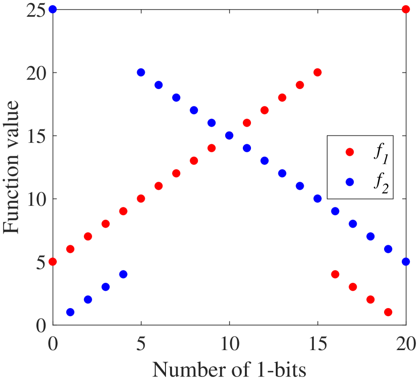
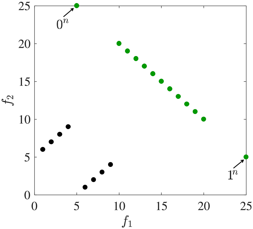
Figure 1: Illustration of the OneJumpZeroJump  problem when $n=20$ and $k=5$. The left subfigure: the function values vs. the number of 1-bits of a solution; the right subfigure: the second function value vs. the first function value, where the set of green points are the Pareto front.

The bi-objective RealRoyalRoad problem dang2023crossover as presented in Definition 2.4 only takes positive function values on two regions $G$ and $H$: $G$ consists of solutions with at most $3n/5$ 1-bits, and $H$ consists of solutions with $4n/5$ 1-bits where all the 1-bits are consecutive. In regions $G$ and $H$, a solution with more 1-bits is preferred, and for two solutions with the same number of 1-bits, the solution with more trailing 0-bits or leading 0-bits is preferred. Note that we use $\textsc{TZ}(\bm{x})=\sum_{i=1}^{n}\prod_{j=i}^{n}(1-x_{j})$ and $\textsc{LZ}(\bm{x})=\sum_{i=1}^{n}\prod_{j=1}^{i}(1-x_{j})$ to denote the number of trailing 0-bits and leading 0-bits of a solution $\bm{x}$, respectively, where $x_{j}$ denotes the $j$-th bit of $\bm{x}\in\{0,1\}^{n}$.

Definition 2.4 (dang2023crossover ).

The bi-objective RealRoyalRoad problem is to find $n$ bits binary strings which maximize

$$f_{1}(\bm{x})=\begin{cases}n|\bm{x}|_{1}+\textsc{TZ}(\bm{x}),&\text{if }\bm{x}\in G\cup H,\\ 0,&\text{else},\end{cases}$$

$$f_{2}(\bm{x})=\begin{cases}n|\bm{x}|_{1}+\textsc{LZ}(\bm{x}),&\text{if }\bm{x}\in G\cup H,\\ 0,&\text{else},\end{cases}$$

where $n/5\in\mathbb{Z}^{+}$, $G=\{\bm{x}\mid|\bm{x}|_{1}\leq 3n/5\}$ and $H=\{\bm{x}\mid|\bm{x}|_{1}=4n/5\wedge\textsc{LZ}(\bm{x})+\textsc{TZ}(\bm{x})=n/5\}$.

From the definition, we can see that the Pareto set of the bi-objective RealRoyalRoad problem is exactly $H$, and the Pareto front is

$$\bm{f}(H)=\Big{\{}\Big{(}\frac{4n^{2}}{5}+a,\frac{4n^{2}}{5}+\frac{n}{5}-a\Big{)}\mid a\in\Big{[}0..\frac{n}{5}\Big{]}\Big{\}},$$ (5)

whose size is $n/5+1$. Figure 2 illustrates the objective vectors and the Pareto front.

Figure 2: The objective vectors of the bi-objective RealRoyalRoad  problem when $n=5$, where the set of green points are the Pareto front.

We use

$$G^{\prime}=\{\bm{x}\mid|\bm{x}|_{1}=3n/5\wedge\textsc{LZ}(\bm{x})+\textsc{TZ}(\bm{x})=2n/5\}$$

to denote the non-dominated set of solutions in $G$.

The OneJumpZeroJump problem characterizes a class of problems where some adjacent Pareto optimal solutions in the objective space locate far away in the decision space, and the bi-objective RealRoyalRoad problem characterizes a class of problems where a large gap exists between Pareto optimal solutions and sub-optimal solutions (i.e., the solutions that can only be dominated by Pareto optimal solutions) in the decision space. Thus, studying these two problems can provide a general insight on the ability of MOEAs of going across inferior regions around Pareto optimal solutions.

3 Running Time Analysis of SMS-EMOA

In this section, we analyze the expected running time of SMS-EMOA in Algorithm 1 using the deterministic population update in Algorithm 2 and the stochastic population update in Algorithm 5 for solving the OneJumpZeroJump and bi-objective RealRoyalRoad problems, which shows that the stochastic population update can bring exponential acceleration. Note that the running time of EAs is often measured by the number of fitness evaluations, which can be the most time-consuming step in the evolutionary process. As SMS-EMOA generates only one offspring solution in each generation, its running time is just equal to the number of generations. Since each objective value of OneJumpZeroJump and bi-objective RealRoyalRoad is not smaller than zero, we set the reference point $\bm{r}=(-1,-1)$.

3.1 Analysis of SMS-EMOA Solving OneJumpZeroJump

First we analyze SMS-EMOA solving the OneJumpZeroJump problem. We prove in Theorems 3.1 and 3.3 that the upper and lower bounds on the expected number of generations of SMS-EMOA using the original population update in Algorithm 2 solving OneJumpZeroJump are $O(\mu n^{k})$ and $\Omega(n^{k})$, respectively. Next, we prove in Theorem 3.4 that by using the stochastic population update in Algorithm 5 to replace the original population update procedure in Algorithm 2, SMS-EMOA can solve OneJumpZeroJump in $O(\mu^{2}n^{k}/2^{k/4})$ expected number of generations, implying a significant acceleration for large $k$.

The main proof idea of Theorem 1 is to divide the optimization procedure into two phases, where the first phase aims at finding the inner part $F_{I}^{*}$ (in Eq. (4)) of the Pareto front, and the second phase aims at finding the remaining two extreme vectors in the Pareto front, i.e., $F^{*}\setminus F_{I}^{*}=\{(k,n+k),(n+k,k)\}$, corresponding to the two Pareto optimal solutions $0^{n}$ and $1^{n}$.

Theorem 3.1.

For SMS-EMOA solving OneJumpZeroJump, if using a population size $\mu$ such that $\mu\geq n-2k+3$, then the expected number of generations for finding the Pareto front is $O(\mu n^{k})$.

Before proving Theorem 3.1, we first present Lemma 3.2, which shows that once an objective vector $\bm{f}^{*}$ in the Pareto front is found, it will always be maintained, i.e., there will always exist a solution in the population whose objective vector is $\bm{f}^{*}$.

Lemma 3.2.

For SMS-EMOA solving OneJumpZeroJump, if using a population size $\mu$ such that $\mu\geq n-2k+3$, then an objective vector $\bm{f}^{*}$ in the Pareto front will always be maintained once it has been found.

Proof.  Suppose the objective vector $(a,n+2k-a),a\in[2k..n]\cup\{k,n+k\}$, in the Pareto front is obtained by SMS-EMOA, i.e., there exists at least one solution in $Q$ (i.e., $P\cup\{\bm{x}^{\prime}\}$ in line 5 of Algorithm 1) corresponding to the objective vector $(a,n+2k-a)$. Note that only one solution is removed in each generation by Algorithm 2, thus we only need to consider the case that exactly one solution (denoted as $\bm{x}^{*}$) corresponds to the objective vector $(a,n+2k-a)$. Since $\bm{x}^{*}$ cannot be dominated by any other solution, we have $\bm{x}^{*}\in R_{1}$ in the Population Update of SMS-EMOA procedure. We also have $\Delta_{\bm{r}}(\bm{x}^{*},R_{1})=HV_{\bm{r}}(R_{1})-HV_{\bm{r}}(R_{1}\setminus\{\bm{x}^{*}\})>0$ because the region

$$\{\bm{f}^{\prime}\in\mathbb{R}^{2}\mid a-1<f^{\prime}_{1}\leq a,n+2k-a-1<f^{\prime}_{2}\leq n+2k-a\}$$ (6)

cannot be covered by any objective vector in $\bm{f}(\{0,1\}^{n})\setminus\{(a,n+2k-a)\}$. Then, we consider two cases.

(1) There exists one solution $\bm{x}$ in $R_{1}$ such that $k\leq|\bm{x}|_{1}\leq n-k$. Then, $R_{1}$ cannot contain solutions whose number of 1-bits are in $[1..k-1]\cup[n-k+1..n-1]$, because these solutions must be dominated by $\bm{x}$. If at least two solutions in $R_{1}$ have the same objective vector, then they must have a zero $\Delta$ value, because removing one of them will not decrease the hypervolume covered. Thus, for each objective vector $(b,n+2k-b),b\in[2k..n]\cup\{k,n+k\}$, at most one solution can have a $\Delta$ value larger than zero, implying that there exist at most $n-2k+3\leq\mu$ solutions in $R_{1}$ with $\Delta>0$.

(2) Any solution $\bm{x}$ in $R_{1}$ satisfies $|\bm{x}|_{1}<k$ or $|\bm{x}|_{1}>n-k$. Note that for the solutions with the number of 1-bits in $[1..k-1]$, a solution with more 1-bits must dominate a solution with less 1-bits. Meanwhile, two solutions with the same number of 1-bits will have a zero $\Delta$ value, thus $R_{1}$ can only contain at most one solution in $\{\bm{x}\mid|\bm{x}|_{1}\in[1..k-1]\}$ with $\Delta$ value larger than zero. Similarly, at most one solution in $\{\bm{x}\mid|\bm{x}|_{1}\in[n-k+1..n-1]\}$ with $\Delta$ value larger than zero belongs to $R_{1}$. For solutions with number of 1-bits in $\{0,n\}$ (note that there may exist reduplicative solutions in $Q$), it is also straightforward to see that at most two of them can have a $\Delta$ value larger than zero. By the problem setting $k<n/2$, we have $\mu\geq n-2k+3\geq 4$, thus there exist at most $\mu$ solutions in $R_{1}$ with $\Delta$ value larger than zero.

Combining the above two cases, we show that there exist at most $\mu$ solutions in $R_{1}$ with $\Delta$ value larger than zero, implying that $\bm{x}^{*}$ will still be maintained in the next generation. $\square$

Proof of Theorem 3.1.  We divide the optimization procedure into two phases. The first phase starts after initialization and finishes until all the objective vectors in the inner part $F_{I}^{*}$ of the Pareto front have been found; the second phase starts after the first phase and finishes when the whole Pareto front is found. We will show that the expected number of generations of the two phases are $O(\mu(n\log n+k^{k}))$ and $O(\mu n^{k})$, respectively, leading to the theorem.

For the first phase, we consider two cases.

(1) At least one solution in the inner part $S_{I}^{*}$ of the Pareto set exists in the initial population. Let

$$D_{1}\!=\!\{\bm{x}\!\in\!P\mid (H^{+}(\bm{x})\cap P=\emptyset\wedge H^{+}(\bm{x})\cap S_{I}^{*}\neq\emptyset)$$ (7)

$$\vee(H^{-}(\bm{x})\cap P=\emptyset\wedge H^{-}(\bm{x})\cap S_{I}^{*}\neq\emptyset)\},$$ (8)

where $H^{+}(\bm{x}):=\{\bm{x}^{\prime}\mid|\bm{x}^{\prime}|_{1}=|\bm{x}|_{1}+1\}$ and $H^{-}(\bm{x}):=\{\bm{x}^{\prime}\mid|\bm{x}^{\prime}|_{1}=|\bm{x}|_{1}-1\}$ denote the Hamming neighbours of $\bm{x}$ with one more 1-bit and one less 1-bit, respectively. Intuitively, $D_{1}$ denotes the set of solutions in $P$ whose Hamming neighbour is Pareto optimal but not contained by $P$. Then, by selecting a solution $\bm{x}\in D_{1}$, and flipping one of the 0-bits or one of the 1-bits, a new objective vector in $F_{I}^{*}$ can be obtained. By Lemma 3.2, one solution corresponding to the new objective vector will always be maintained in the population. Then, by repeating the above procedure, the whole set $F_{I}^{*}$ can be found. Note that the probability of selecting a specific solution in $P$ is $1/\mu$, and the probability of flipping one of the 0-bits (or 1-bits) is $(n-|\bm{x}|_{1})\cdot(1/n)\cdot(1-1/n)^{n-1}\geq(n-|\bm{x}|_{1})/(en)$ (or $(|\bm{x}|_{1}/n)\cdot(1-1/n)^{n-1}\geq|\bm{x}|_{1}/(en)$). Thus, the total expected number of generations for finding $F_{I}^{*}$ is at most $\sum^{|\bm{x}|_{1}}_{i=k+1}(\mu en)/i+\sum^{n-|\bm{x}|_{1}}_{i=k+1}(\mu en)/i=O(\mu n\log n)$.

(2) Any solution in the initial population has at most $(k-1)$ 1-bits or at least $(n-k+1)$ 1-bits. Without loss of generality, we can assume that one solution $\bm{y}$ has at most $(k-1)$ 1-bits. Then, selecting $\bm{y}$ and flipping $(k-|\bm{y}|_{1})$ 0-bits can generate a solution in $S_{I}^{*}$, whose probability is at least

$$\frac{1}{\mu}\cdot\frac{\binom{n-|\bm{y}|_{1}}{k-|\bm{y}|_{1}}}{n^{k-|\bm{y}|_{1}}}\cdot\Big{(}1-\frac{1}{n}\Big{)}^{n-k+|\bm{y}|_{1}}\geq\frac{1}{e\mu}\cdot\frac{\binom{n-|\bm{y}|_{1}}{k-|\bm{y}|_{1}}}{n^{k-|\bm{y}|_{1}}}.$$ (9)

Let $g(i)=\binom{n-i}{k-i}/n^{k-i},0\leq i\leq k-1$, then we have

$$\frac{g(i+1)}{g(i)}=\frac{\binom{n-i-1}{k-i-1}}{\binom{n-i}{k-i}}\cdot n=\frac{n(k-i)}{(n-i)}\geq 1,$$ (10)

implying

$$\frac{\binom{n-|\bm{y}|_{1}}{k-|\bm{y}|_{1}}}{n^{k-|\bm{y}|_{1}}}=g(|\bm{y}|_{1})\geq g(0)=\frac{\binom{n}{k}}{n^{k}}\geq\Big{(}\frac{n}{k}\Big{)}^{k}\cdot\frac{1}{n^{k}}=\frac{1}{k^{k}}.$$ (11)

Thus, the expected number of generations for finding a solution in $S_{I}^{*}$ is at most $e\mu k^{k}$. By Lemma 3.2, the generated solution must be included into the population. Thus, combining the analysis for case (1), we can derive that the total expected number of generations for finding $F_{I}^{*}$ is $O(\mu(n\log n+k^{k}))$.

For the second phase, we need to find the two extreme solutions $\!1^{n}\!$ and $\!0^{n}\!$. To find $1^{n}$ (or $0^{n}$), it is sufficient to select the solution in the population $P$ with $(n-k)$ 1-bits (or $k$ 1-bits) and flip its $k$ 0-bits (or $k$ 1-bits), whose probability is $(1/\mu)\cdot(1/n^{k})\cdot(1-1/n)^{n-k}\geq 1/(e\mu n^{k})$. Thus, the expected number of generations is $O(e\mu n^{k})$.

Combining the analysis of the two phases, the expected number of generations for finding the whole Pareto front is $O(\mu(n\log n+k^{k}))+O(e\mu n^{k})=O(\mu n^{k})$. $\square$

The proof idea of Theorem 3.3 is that all the solutions in the initial population belong to the inner part $S_{I}^{*}$ (in Eq. (3)) of the Pareto set with probability $\Theta(1)$, and then SMS-EMOA requires $\Omega(n^{k})$ expected number of generations to find the two extreme Pareto optimal solutions $1^{n}$ and $0^{n}$.

Theorem 3.3.

For SMS-EMOA solving OneJumpZeroJump with $n-2k=\Omega(n)$, if using a population size $\mu$ such that $\mu=poly(n)$, then the expected number of generations for finding the Pareto front is $\Omega(n^{k})$.

Proof.  Let $A$ denote the event that all the solutions in the initial population belong to $S_{I}^{*}$, i.e., for any solution $\bm{x}$ in the initial population, $k\leq|\bm{x}|_{1}\leq n-k$. We first show that event $A$ happens with probability $1-o(1)$. For an initial solution $\bm{y}$, it is generated uniformly at random, i.e., each bit in $\bm{y}$ can be 1 or 0 with probability $1/2$, respectively. Thus, the expected number of 1-bits in $\bm{y}$ is exactly $n/2$. By Hoeffding’s inequality and the condition $n-2k=\Omega(n)$ of the theorem, we have

$$\Pr\Big{(}\Big{|}|\bm{y}|_{1}-\frac{n}{2}\Big{|}>\frac{n}{2}-k\Big{)}<2e^{-2(n/2-k)^{2}/n}=e^{-\Omega(n)}.$$ (12)

Then, we can derive that

$$\Pr\Big{(}\forall\bm{x}\text{ in the initial population},\Big{|}|\bm{x}|_{1}-\frac{n}{2}\Big{|}\leq\frac{n}{2}-k\Big{)}$$ (13)

$$\geq\big{(}1-e^{-\Omega(n)}\big{)}^{\mu}\geq 1-\mu\cdot e^{-\Omega(n)}=1-o(1),$$ (14)

where the last inequality holds by Bernoulli’s inequality, and the equality holds by the condition $\mu=poly(n)$.

Next we show that given event $A$, the expected number of generations for finding the whole Pareto front is at least $n^{k}$. Starting from the initial population, if a solution $\bm{x}$ with $1\leq|\bm{x}|_{1}\leq k-1$ or $n-k+1\leq|\bm{x}|_{1}\leq n-1$ is generated in some generation, it must be deleted because it is dominated by any of the solutions in the current population. Thus, the extreme solution $1^{n}$ can only be generated by selecting a solution in $S_{I}^{*}$ and flipping all the 0-bits, whose probability is at most $1/n^{k}$. Thus, the expected number of generations for finding $1^{n}$ is at least $n^{k}$.

Combining the above analyses, the expected number of generations for finding the whole Pareto front is at least $(1-o(1))\cdot n^{k}=\Omega(n^{k})$. $\square$

The basic proof idea of Theorem 3.4 is similar to that of Theorem 3.1, i.e., dividing the optimization procedure into two phases, which are to find $F_{I}^{*}$ and $F^{*}\setminus F_{I}^{*}=\{(k,n+k),(n+k,k)\}$, respectively. However, the analysis for the second phase is a little more sophisticated here, because dominated solutions can be included into the population when using the stochastic population update, leading to a more complicated behavior of SMS-EMOA.

Theorem 3.4.

For SMS-EMOA solving OneJumpZeroJump, if using the stochastic population update in Algorithm 5, and a population size $\mu$ such that $\mu\geq 2(n-2k+4)$, then the expected number of generations for finding the Pareto front is $O(\mu^{2}n^{k}/2^{k/4})$.

Before proving Theorem 3.4, we first present Lemma 3.5, which shows that given proper value of $\mu$, an objective vector in the Pareto front will always be maintained once it has been found; any solution (even the worst solution) in the collections of the current population and the newly generated offspring solution can survive in the population update procedure with probability at least $1/2$.

Lemma 3.5.

For SMS-EMOA solving OneJumpZeroJump, if using the stochastic population update in Algorithm 5, and a population size $\mu$ such that $\mu\geq 2(n-2k+4)$, then

• an objective vector $\bm{f}^{*}$ in the Pareto front will always be maintained once it has been found;

• any solution in $P\cup\{\bm{x}^{\prime}\}$ can be maintained in the next population with probability at least $1/2$, where $P$ denotes the current population and $\bm{x}^{\prime}$ denotes the offspring solution produced in the current generation.

Proof.  The proof of the first clause is similar to that of Lemma 3.2. Suppose that one solution $\bm{x}^{*}$ corresponding to $\bm{f}^{*}$ exists in $Q=P\cup\{\bm{x}^{\prime}\}$. By the proof of Lemma 3.2, there exist at most $n-2k+3$ solutions in $R_{1}$ with $\Delta$ value larger than zero. Note that the removed solution is chosen from $\lfloor(\mu+1)/2\rfloor\geq n-2k+4$ solutions in $Q$, thus $\bm{x}^{*}$ will not be removed because it is one of the best $n-2k+3$ solutions. Then, the first clause holds.

The second clause holds, because for any solution in $P\cup\{\bm{x}^{\prime}\}$, it can be removed only if it is chosen for competition, whose probability is at most $\lfloor(\mu+1)/2\rfloor/(\mu+1)\leq 1/2$. $\square$

Then, we present Lemma 3.6, which is used to derive an upper bound on the expected number of generations of the second phase. Because the population of SMS-EMOA in the $(t+1)$-th generation only depends on the $t$-th population, its process can be naturally modeled as a Markov chain. Given a Markov chain $\{\xi_{t}\}^{+\infty}_{t=0}$ and $\xi_{\hat{t}}=\mathrm{x}\in\mathcal{X}$, we define its first hitting time as $\tau=\min\{t\mid\xi_{\hat{t}+t}\in\mathcal{X}^{*},t\geq 0\}$, where $\mathcal{X}$ and $\mathcal{X}^{*}$ denote the state space and target state space of the Markov chain, respectively. For the analysis in Theorem 3.4, $\mathcal{X}$ denotes the set of all the populations after phase 1, and $\mathcal{X}^{*}$ denotes the set of all the populations which contain the Pareto optimal solution $1^{n}$ (or $0^{n}$). The mathematical expectation of $\tau$, $\mathbb{E}(\tau\mid\xi_{\hat{t}}=\mathrm{x})=\sum\nolimits^{+\infty}_{i=0}i\cdot\Pr(\tau=i\mid\xi_{\hat{t}}=\mathrm{x})$, is called the expected first hitting time (EFHT) starting from $\xi_{\hat{t}}=\mathrm{x}$. The additive drift as presented in Lemma 3.6 is used to derive upper bounds on the EFHT of Markov chains. To use it, a function $V(\mathrm{x})$ has to be constructed to measure the distance of a state $\mathrm{x}$ to the target state space $\mathcal{X}^{*}$, where $V(\mathrm{x}\in\mathcal{X}^{*})=0$ and $V(\mathrm{x}\notin\mathcal{X}^{*})>0$. Then, we need to investigate the progress on the distance to $\mathcal{X}^{*}$ in each step, i.e., $\mathbb{E}(V(\xi_{t})-V(\xi_{t+1})\mid\xi_{t})$. An upper bound on the EFHT can be derived through dividing the initial distance by a lower bound on the progress.

Lemma 3.6 (Additive Drift he2001drift ).

Given a Markov chain $\{\xi_{t}\}^{+\infty}_{t=0}$ and a distance function $V(\cdot)$, if for any $t\geq 0$ and any $\xi_{t}$ with $V(\xi_{t})>0$, there exists a real number $c>0$ such that $\mathbb{E}(V(\xi_{t})-V(\xi_{t+1})\mid\xi_{t})\geq c$, then the EFHT satisfies that $\mathbb{E}(\tau\mid\xi_{0})\leq V(\xi_{0})/c.$

Proof of Theorem 3.4.  Similar to the proof of Theorem 3.1, we divide the optimization procedure into two phases. That is, the first phase starts after initialization and finishes until all the objective vectors in $F_{I}^{*}$ have been found; the second phase starts after the first phase and finishes when $0^{n}$ and $1^{n}$ are also found. The analysis of the first phase is the same as that of Theorem 3.1, because the objective vectors in $F_{I}^{*}$ will always be maintained by Lemma 3.5. That is, the expected number of generations of phase 1 is $O(\mu(n\log n+k^{k}))$.

Now we analyze the second phase. Without loss of generality, we only consider the expected number of generations for finding $1^{n}$, and the same bound holds for finding $0^{n}$ analogously. We use Lemma 3.6, i.e., additive drift analysis, to prove. Note that the process of SMS-EMOA can be directly modeled as a Markov chain by letting the state of the chain represent a population of SMS-EMOA. Furthermore, the target space consists of all the populations which contain $1^{n}$. In the following, we don’t distinguish a state from its corresponding population. First, we construct the distance function

$$V(P)=\begin{cases}0&\text{if }\max_{\bm{x}\in P}|\bm{x}|_{1}=n,\\ e\mu n^{k/2}&\text{if }n-k/2\leq\max_{\bm{x}\in P}|\bm{x}|_{1}\leq n\!-\!1,\\ e\mu n^{k/2}+1&\text{if }n-k\leq\max_{\bm{x}\in P}|\bm{x}|_{1}<n-k/2.\end{cases}$$ (15)

It is easy to verify that $V(P)=0$ if and only if $1^{n}\in P$.

Then, we examine $\mathbb{E}(V(\xi_{t})-V(\xi_{t+1})\mid\xi_{t}=P)$ for any $P$ with $1^{n}\notin P$. Assume that currently $\max_{\bm{x}\in P}|\bm{x}|_{1}=q$, where $n-k\leq q\leq n-1$. We first consider the case that $n-k/2\leq q\leq n-1$. To make $V$ decrease, it is sufficient to select the solution in $P$ with $q$ 1-bits and flip its remaining $(n-q)$ 0-bits, whose probability is $(1/{\mu})\cdot(1/{n^{n-q}})\cdot(1-1/n)^{q}\geq 1/({e\mu n^{n-q}})\geq 1/(e\mu n^{k/2})$, where the last inequality is by $n-k/2\leq q$. Note that the newly generated solution is $1^{n}$, which must be included in the population. In this case, $V$ can decrease by $e\mu n^{k/2}$. To make $V$ increase, the solution in $P$ with $q$ 1-bits needs to removed in the next generation, whose probability is at most $1/2$ by Lemma 3.5. In this case, $V$ can increase by $e\mu n^{k/2}+1-e\mu n^{k/2}=1$. Thus, we have

$$\mathbb{E}(V(\xi_{t})-V(\xi_{t+1})\mid\xi_{t}=P)\geq\frac{e\mu n^{k/2}}{e\mu n^{k/2}}-\frac{1}{2}\cdot 1\geq\frac{1}{2}.$$ (16)

Now we consider the case that $n-k\leq q<n-k/2$. Note that in this case, $V$ cannot increase, thus we only need to consider the decrease of $V$. We further consider two subcases.
(1) $q>n-3k/4$. To make $V$ decrease by $1$, it is sufficient to select the solution with $q$ 1-bits, flip $k/4$ 0-bits among the $(n-q)$ 0-bits, and include the newly generated solution into the population, whose probability is at least $(1/\mu)\cdot(\binom{n-q}{k/4}/{n^{k/4}})\cdot(1-1/n)^{n-k/4}\cdot(1/2)\geq\binom{k/2}{k/4}/(2e\mu n^{k/4})$. Thus, $\mathbb{E}(V(\xi_{t})-V(\xi_{t+1})\mid\xi_{t}=P)\geq\binom{k/2}{k/4}/{(2e\mu n^{k/4})}$.
(2) $q\leq n-3k/4$. To make $V$ decrease by $1$, it is sufficient to select the solution with $q$ 1-bits, flip $(n-k/2-q)$ 0-bits among the $(n-q)$ 0-bits, and include the newly generated solution into the population, whose probability is at least

$$\frac{1}{\mu}\cdot\frac{\binom{n-q}{n-k/2-q}}{n^{n-k/2-q}}\cdot\Big{(}1-\frac{1}{n}\Big{)}^{k/2+q}\cdot\frac{1}{2}\geq\frac{\binom{n-q}{k/2}}{2e\mu n^{k/2}}\geq\frac{\binom{3k/4}{k/2}}{2e\mu n^{k/2}}\geq\frac{\binom{k/2}{k/4}}{2e\mu n^{k/2}},$$ (17)

where the first inequality is by $n-k\leq q$. Thus, $\mathbb{E}(V(\xi_{t})-V(\xi_{t+1})\mid\xi_{t}=P)\geq\binom{k/2}{k/4}/({2e\mu n^{k/2}})$.
Combining subcases (1) and (2), we can derive

$$\mathbb{E}(V(\xi_{t})-V(\xi_{t+1})\mid\xi_{t}=P)\geq\frac{\binom{k/2}{k/4}}{2e\mu n^{k/2}}\geq\frac{2^{k/4}}{2e\mu n^{k/2}}.$$ (18)

By Eqs. (16) and (18), we have $\mathbb{E}(V(\xi_{t})-V(\xi_{t+1})\mid\xi_{t}=P)\geq 2^{k/4}/(2e\mu n^{k/2})$. Then, by Lemma 3.6 and $V(P)\leq e\mu n^{k/2}+1$, the expected number of generations for finding $1^{n}$ is at most $(e\mu n^{k/2}+1)\cdot(2e\mu n^{k/2})/2^{k/4}=O(\mu^{2}n^{k}/2^{k/4})$.

Thus, combining the two phases, the expected number of generations for finding the whole Pareto front is $O(\mu(n\log n+k^{k}))+O(\mu^{2}n^{k}/2^{k/4})=O(\mu^{2}n^{k}/2^{k/4})$, where the equality holds by $2\leq k<n/2$. Thus, the theorem holds. $\square$

Comparing the results of Theorems 3.3 and 3.4, we can find that when $k=\Omega(n)\wedge k=n/2-\Omega(n)$ and $2(n-2k+4)\leq\mu=poly(n)$, using the stochastic population update can bring an acceleration of $\Omega(2^{k/4}/\mu^{2})$, i.e., exponential acceleration. The main reason for the acceleration is that introducing randomness into the population update procedure can make SMS-EMOA go across inferior regions between different Pareto optimal solutions more easily. Specifically, the original deterministic population update method prefers non-dominated solutions; thus for OneJumpZeroJump whose objective vectors in the Pareto front are far away in the solution space, SMS-EMOA is easy to get trapped. However, the stochastic population update method allows dominated solutions (i.e., solutions with the number of 1-bits in $[1..k-1]\cup[n-k+1..n-1]$), to participate in the evolutionary process, thus making SMS-EMOA able to follow an easier path in the solution space to find the extreme Pareto optimal solutions $0^{n}$ and $1^{n}$.

3.2 Analysis of SMS-EMOA Solving Bi-objective RealRoyalRoad

Now we analyze SMS-EMOA solving the bi-objective RealRoyalRoad problem. We prove in Theorems 3.7 and 3.9 that the upper and lower bounds on the expected number of generations of SMS-EMOA using the original population update in Algorithm 2 solving bi-objective RealRoyalRoad are $O(\mu n^{n/5-2})$ and $\Omega(n^{n/5-1})$, respectively. We also prove in Theorem 3.10 that by using the stochastic population update in Algorithm 5 to replace the original population update procedure in Algorithm 2, SMS-EMOA can solve bi-objective RealRoyalRoad in $O(\mu^{2}n^{n/5}/2^{n/20}\})$ expected number of generations, implying an exponential acceleration for $\mu=poly(n)$. Note that we use $poly(n)$ to denote any polynomial of $n$.

The proof of Theorem 3.7 is inspired by that of Theorem 6 in dang2023crossover . That is, we divide the optimization procedure into five phases, where the first phase aims at finding a solution with $3n/5$ 1-bits, the second phase aims at finding a solution in $G^{\prime}=\{\bm{x}\mid|\bm{x}|_{1}=3n/5\wedge\textsc{LZ}(\bm{x})+\textsc{TZ}(\bm{x})=2n/5\}$, the third phase aims at finding all the solutions in $G^{\prime}$, the fourth phase aims at finding a solution in $H=\{\bm{x}\mid|\bm{x}|_{1}=4n/5\wedge\textsc{LZ}(\bm{x})+\textsc{TZ}(\bm{x})=n/5\}$ (i.e., a Pareto optimal solution), and the fifth phase aims at finding all the solutions in $H$ (i.e., all the Pareto optimal solutions).

Theorem 3.7.

For SMS-EMOA solving bi-objective RealRoyalRoad, if using a population size $\mu$ such that $\mu\geq 2n/5+1$, then the expected number of generations for finding the Pareto front is $O(\mu n^{n/5-2})$.

Before proving Theorem 3.7, we first present Lemma 3.8, which shows that once a solution is found, then a weakly dominating solution will always be maintained in the population.

Lemma 3.8.

For SMS-EMOA solving bi-objective RealRoyalRoad, if using a population size $\mu$ such that $\mu\geq 2n/5+1$, then

• if a solution with $i$ ($i\leq 3n/5$) 1-bits is found and any solution in $H$ is not found, then a solution with $j$ ($i\leq j\leq 3n/5$) 1-bits will always be maintained in the population;

• if a solution $\bm{x}\in G^{\prime}$ is found and any solution in $H$ is not found, then $\bm{x}$ will always be maintained in the population;

• if a solution in $H$ is found, then it will always be maintained in the population.

Proof.  First we consider the first clause. Suppose a solution $\bm{x}$ with $i$ 1-bits ($1\leq i\leq 3n/5$) is found. If $\bm{x}\in R_{s}$ ($s\geq 2$) in the population update procedure, i.e., $\bm{x}$ is dominated by a solution $\bm{y}$, then $\bm{y}$ must have $j$ ($i\leq j\leq 3n/5$) 1-bits. Note that only one solution in the last non-dominated set $R_{v}$ will be removed in the population update procedure, thus $\bm{y}$ must be maintained, implying that the claim holds. If $\bm{x}\in R_{1}$, i.e., $\bm{x}$ is non-dominated, then $\bm{x}$ can be removed only if all the solutions in $Q$ (i.e., the union of the current population and the newly generated solution) belong to $R_{1}$. Then, by the definition of bi-objective RealRoyalRoad, all the solutions in $Q$ must have $i$ 1-bits. Thus, the claim also holds.

Now we consider the second clause. Note that only one solution will be removed in each generation, thus we only need to consider the case that any solution $\bm{y}\in Q$ is different from $\bm{x}$. By the definition of bi-objective RealRoyalRoad, we can see that $\bm{x}$ cannot be dominated by any other solution in $Q$, thus $\bm{x}\in R_{1}$ in the Population Update of SMS-EMOA procedure. Meanwhile, similar to the analysis of Eq. (6), there must exist a region around $\bm{f}(\bm{x})$ that cannot be covered by any objective vector in $\bm{f}(Q\setminus\{\bm{x}\})$, implying $\Delta_{\bm{r}}(\bm{x},R_{1})=HV_{\bm{r}}(R_{1})-HV_{\bm{r}}(R_{1}\setminus\{\bm{x}\})>0$. Note that any solution with less than $3n/5$ 1-bits or more than $3n/5$ 1-bits must be dominated by $\bm{x}$ (note that we assume that the solutions in $H$ are not found), thus $R_{1}$ can only consist of solutions with $3n/5$ 1-bits. For any solution with $3n/5$ 1-bits, their first objective value can only have at most $(2n/5+1)$ different choices, thus the number of different objective vectors of the solutions in $R_{1}$ is at most $2n/5+1$. If at least two solutions in $R_{1}$ have the same objective vector, then they must have a zero $\Delta$ value, because removing one of them will not decrease the hypervolume covered. Thus, there exist at most $2n/5+1\leq\mu$ solutions in $R_{1}$ with $\Delta$ value larger than zero, implying $\bm{x}$ will be maintained in the next population.

The proof of the third clause is similar to that of the second clause, and the main difference is that there exist at most $(n/5+1)$ solutions in $R_{1}$ with $\Delta$ value larger than zero, which will not influence the analysis. Combining the three cases, the lemma holds. $\square$

Proof of Theorem 3.7.  We divide the optimization procedure into five phases, and derive the expected number of generations of each phase separately, whose sum will result in the upper bound on the total expected number of generations. Note that in the following analysis, we assume that there exists a solution in the initial population which has at most $3n/5$ 1-bits (i.e., belongs to $G=\{\bm{x}\mid|\bm{x}|_{1}\leq 3n/5\}$), and the analysis of the other case is put in the end of the proof. We also pessimistically assume that in the analysis of phases 1-3, any solution in $H$ is not maintained in the population, because otherwise the analysis can directly move to phase 4.

The first phase: a solution with exactly $3n/5$ 1-bits is maintained in the population. Assume that $\max_{\bm{x}\in P\cap G}|\bm{x}|_{1}=i$, $i<3n/5$, where $P$ denotes the current population, and let $\bm{x}^{*}$ be one corresponding solution. Then, by selecting $\bm{x}^{*}$ and flipping one of the 0-bits, a solution in $G$ with $(i+1)$ 1-bits can be generated. Thus, by the first clause of Lemma 3.8, a solution with $j$ ($i+1\leq j\leq 3n/5$) 1-bits will be maintained in the population. By repeating the above procedure, a solution with exactly $3n/5$ 1-bits can be found. Note that the probability of selecting a specific solution in $P$ is $1/\mu$, the probability of flipping one of the 0-bits is $(n-|\bm{x}^{*}|_{1})\cdot(1/n)\cdot(1-1/n)^{n-1}\geq(n-i)/(en)$, thus the total expected number of generations of this phase is at most $\sum_{i=0}^{3n/5-1}(\mu en)/(n-i)=O(\mu n\log n)$.

The second phase: a solution in $G^{\prime}$ is maintained in the population. First, we show that the maximal $f_{1}$ value, i.e., $n|\cdot|_{1}+\textsc{TZ}(\cdot)$, will not decrease. Let $D$ denote the set of solutions in $P$ with the maximal $f_{1}$ value. If $D$ contains at least two solutions, then the claim must hold because only one solution will be removed in each generation. If $D$ contains only one solution, then the solution must belong to $R_{1}$ and have a positive $\Delta$ value. Note that a solution with exactly $3n/5$ 1-bits has been found and any solution in $H$ is not found, thus the solutions in $R_{1}$ must have exactly $3n/5$ 1-bits, implying that they can have at most $2n/5+1$ different $f_{1}$ values. Note that for each $f_{1}$ value, only one corresponding solution can belong to $R_{1}$ and have a positive $\Delta$ value. Thus, the solution in $D$ is among the best $2n/5+1\leq\mu$ solutions, and thus will not be removed.
Now, we analyze the expected number of generations for finding a solution in $G^{\prime}$. Assume that $\max_{\bm{x}\in P,|\bm{x}|_{1}=3n/5}f_{1}(\bm{x})=i$, $i<3n^{2}/5+2n/5$, and let $\bm{x}^{*}$ denote a corresponding solution. Then, by selecting $\bm{x}^{*}$ and flipping the last 1-bit as well as one 0-bit before the last 1-bit, a solution with $3n/5$ 1-bits and more trailing 0-bits can be generated. Note that the probability of selecting a specific solution in $P$ is $1/\mu$, and the probability of flipping the desired 1-bit and 0-bit is $(1/n^{2})\cdot(1-1/n)^{n-2}\geq 1/(en^{2})$. Thus, the expected number of generations to increase $f_{1}$ by 1 is at most $\mu en^{2}$. To find a solution in $G^{\prime}$, it is sufficient to increase $f_{1}$ at most $2n/5$ times (in this case, the solution $1^{3n/5}0^{2n/5}$ can be found). Thus, the total expected number of generations of this phase is at most $\mu en^{2}\cdot(2n/5)=O(\mu n^{3})$.

The third phase: the whole $G^{\prime}$ is maintained in the population. Suppose $G^{\prime}$ is not covered, then there exists a solution $\bm{y}\in G^{\prime}\setminus P$ which can be generated from a solution $\bm{x}\in G^{\prime}\cap P$ by flipping the first 1-bit in the solution and the first 0-bit in the trailing 0-bits string, or flipping the last 1-bit in the solution and the last 0-bit in the leading 0-bits string. By the second clause in Lemma 3.8, $\bm{y}$ will be included in the next population. Then, the whole $G^{\prime}$ can be found by repeating the above procedure at most $2n/5$ times. Note that the probability of selecting a specific solution in $P$ is $1/\mu$, the probability of flipping the desired 1-bit and 0-bit is $(1/n^{2})\cdot(1-1/n)^{n-2}\geq 1/(en^{2})$, thus the total expected number of generations of this phase is at most $\mu en^{2}\cdot 2n/5=O(\mu n^{3})$.

The fourth phase: a solution in $H$ is maintained in the population. Let $G^{\prime\prime}:=\{0^{i}1^{3n/5}0^{2n/5-i}\mid n/10\leq i\leq 3n/10\}$ denote the subset of $G^{\prime}$. For each $\bm{x}=0^{i}1^{3n/5}0^{2n/5-i},n/10\leq i\leq n/5$, flipping the consecutive $j$ 0-bits ($j\leq i$) before the 1-bits string and the consecutive $(n/5-j)$ 0-bits after the 1-bits string can generate a solution in $H$. That is, there are $i\geq 10/n$ different ways to generate a solution in $H$. Similarly, for each $\bm{x}=0^{i}1^{3n/5}0^{2n/5-i},n/5<i\leq 3n/10$, flipping the consecutive $j$ 0-bits ($j\leq 2n/5-i$) after the 1-bits string and the consecutive $(n/5-j)$ 0-bits before the 1-bits string can generate a solution in $H$. That is, there are $2n/5-i\geq 10/n$ different ways to generate a solution in $H$. Thus, once a solution in $G^{\prime\prime}$ is selected, the probability of generating a solution in $H$ is at least $n/10\cdot 1/n^{n/5}\cdot(1-1/n)^{4n/5}\geq 1/(10en^{n/5-1})$. Note that the size of $G^{\prime\prime}$ is $n/5+1$, we can derive that the probability of generating a solution in $H$ is at least $(n/5+1)/\mu\cdot 1/(10en^{n/5-1})$ in each generation, implying an upper bound $O(\mu n^{n/5-2})$ on the expected number of generations of this phase.

The fifth phase: the whole $H$ is maintained in the population. The proof is almost the same as that of the third phase, except that we only need to find at most $n/5$ remaining solutions in $H$. Thus, we can directly derive that the total expected number of generations of this phase is at most $\mu en^{2}\cdot n/5=O(\mu n^{3})$.

Combining all the phases, the total expected number of generations is $O(\mu n^{n/5-2})$. Note that such upper bound relies on the assumption that there exists a solution in the initial population which has at most $3n/5$ 1-bits. Now we consider the case that all the solutions in the initial population have more than $3n/5$ 1-bits. By Chernoff bound, the probability that an initial solution has more than $3n/5$ 1-bits is at most $2^{-\Omega(n)}$. Let $B$ denote the event that all the initial solutions have more than $3n/5$ 1-bits, then we have $\Pr(B)=2^{-\Omega(\mu n)}$. If $B$ happens, by selecting any solution in the population, and flipping at most $2n/5$ 1-bits, a solution with at most $3n/5$ 1-bits can be found, whose probability is at least $(1/n^{2n/5})\cdot(1-1/n)^{3n/5}\geq 1/(en^{2n/5})$. After finding a solution with at most $3n/5$ 1-bits, we can directly use the above analysis of the five phases. Thus, the expected number of generations when $B$ happens is at most $en^{2n/5}+O(\mu n^{n/5-2})$. Now, by the law of total expectation, we have

$$\mathbb{E}(T) =\mathbb{E}(T|\neg B)\cdot\Pr(\neg B)+\mathbb{E}(T|B)\cdot\Pr(B)$$ (19)

$$\leq\mathbb{E}(T|\neg B)+\mathbb{E}(T|B)\cdot\Pr(B)$$ (20)

$$\leq O(\mu n^{n/5-2})+\big{(}en^{2n/5}+O(\mu n^{n/5-2})\big{)}\cdot 2^{-\Omega(\mu n)}$$ (21)

$$=O(\mu n^{n/5-2})+en^{2n/5}\cdot 2^{-\Omega(\mu n)}=O(\mu n^{n/5-2}),$$ (22)

where the last equality is by $\mu\geq 2n/5+1$. Thus, the theorem holds. $\square$

From the above proof, we can find that compared with Theorem 6 in dang2023crossover , there are still some differences in the proof procedure. First, instead of GSEMO, we analyze SMS-EMOA here, which employs different population update methods. Second, the crossover operator is not used in SMS-EMOA. Furthermore, due to the difference in population update, the analysis of the first phase in dang2023crossover , (i.e., finding a solution with at most $3n/5$ 1-bits), does not hold anymore, and we use the law of total expectation to handle the running time in this phase.

The proof idea of Theorem 3.9 is similar to that of Theorem 3.3. That is, all the solutions in the initial population have at most $3n/5$ 1-bits with large probability, and then SMS-EMOA needs to flip $n/5$ 0-bits of a solution simultaneously to find a Pareto optimal solution, leading to a large running time.

Theorem 3.9.

For SMS-EMOA solving bi-objective RealRoyalRoad, if using a population size $\mu$ such that $\mu=poly(n)$, then the expected number of generations for finding the Pareto front is $\Omega(n^{n/5-1})$.

Proof.  Let $A$ denote the event that all the initial solutions have at most $3n/5$ 1-bits. By Chernoff bound, the probability that an initial solution has more than $3n/5$ 1-bits is at most $2^{-\Omega(n)}$, thus

$$\Pr(A)\geq(1-2^{-\Omega(n)})^{\mu}\geq 1-\mu\cdot 2^{-\Omega(n)}=1-o(1),$$

where the last inequality is by Bernoulli’s inequality, and the equality is by the condition $\mu=poly(n)$.

Next we show that given event $A$, the expected number of generations for finding a solution in $H$ is $\Omega(n^{n/5-1})$. Starting from the initial population, if a solution $\bm{x}\notin H$ with $|\bm{x}|_{1}>3n/5$ is generated in some generation, it must be deleted because it is dominated by any of the solutions in the current population. Note that any solution in the population has at most $3n/5$ 1-bits, and any solution in $H$ has $4n/5$ 1-bits. Thus, given any solution $\bm{x}$ in the population, the probability of generating a specific solution in $H$ from $\bm{x}$ by mutation is at most $1/n^{n/5}$. Note that the size of $H$ is $n/5+1$, thus the probability of generating a solution in $H$ from $\bm{x}$ is at most $(n/5+1)/n^{n/5}$, implying that the expected number of generations is at least $\Omega(n^{n/5-1})$.

Combining the above analyses, the expected number of generations for finding the Pareto front is at least $(1-o(1))\cdot\Omega(n^{n/5-1})=\Omega(n^{n/5-1})$. $\square$

The proof idea of Theorem 3.10 is similar to that of Theorem 3.7, i.e., dividing the optimization procedure into five phases. However, for the fourth phase, we use additive drift analysis to prove, just as the analysis of the second phase in the proof of Theorem 3.4.

Theorem 3.10.

For SMS-EMOA solving bi-objective RealRoyalRoad, if using the stochastic population update in Algorithm 5, and a population size $\mu$ such that $\mu\geq 2(2n/5+2)$, then the expected number of generations for finding the Pareto front is $O(\mu^{2}n^{n/5}/2^{n/20})$.

Before proving Theorem 3.10, we first present Lemma 3.11, which shows that given proper value of $\mu$, then once a solution is found, a weakly dominating solution will always be maintained in the population; any solution in the collections of the current population and the newly generated offspring solution can survive in the population update procedure with probability at least $1/2$.

Lemma 3.11.

For SMS-EMOA solving bi-objective RealRoyalRoad, if using the stochastic population update in Algorithm 5, and a population size $\mu$ such that $\mu\geq 2(2n/5+2)$, then the three clauses in Lemma 3.8 holds, and we further have

• any solution in $P\cup\{\bm{x}^{\prime}\}$ can be maintained in the next population with probability at least 1/2, where $P$ denotes the current population and $\bm{x}^{\prime}$ denotes the offspring solution produced in the current generation.

Proof.  For the first clause, the proof is the same as that of Lemma 3.8. For the proofs of the second and the third clauses, we can see from Lemma 3.8 that there exist at most $2n/5+1$ solutions in $R_{1}$ with $\Delta$ value larger than zero, implying that the found solution $\bm{x}$ is among the best $2n/5+1$ solutions if it is selected for competition. Note that the number of solutions selected for competition in line 1 of Algorithm 5 is $\lfloor(\mu+1)/2\rfloor\geq 2n/5+2$, thus $\bm{x}$ must not be the worst solution and thus will not be removed. The proof of the new clause is the same as the second clause of Lemma 3.5. $\square$

Proof of Theorem 3.10.  Similar to the proof of Theorem 3.7, we divide the optimization procedure into five phases. The analysis of the first, second, third and fifth phases is the same as that of Theorem 3.7, because the stochastic population update does not affect the selection and mutation operator, and Lemma 3.8 can be directly replaced by Lemma 3.11. The main difference is the analysis of the fourth phase, i.e., finding a solution in $H=\{\bm{x}\mid|\bm{x}|_{1}=4n/5\wedge\textsc{LZ}(\bm{x})+\textsc{TZ}(\bm{x})=n/5\}$ after all the solutions in $G^{\prime}=\{\bm{x}\mid|\bm{x}|_{1}=3n/5\wedge\textsc{LZ}(\bm{x})+\textsc{TZ}(\bm{x})=2n/5\}$ are maintained in the population. We will show that the expected number of generations of the fourth phase can be improved from $O(\mu n^{n/5-2})$ to $O(\mu^{2}n^{n/5}/2^{n/20})$, whose proof is accomplished by using Lemma 3.6, i.e., additive drift analysis.

Let $D=\{\bm{x}\in\{0,1\}^{n}\mid\textsc{LZ}(\bm{x})+\textsc{TZ}(\bm{x})\geq n/5\}$. We first construct a distance function $V(P)$ as,

$$V(P)=\begin{cases}0&\text{if }\max_{\bm{x}\in P\cap D}|\bm{x}|_{1}=4n/5,\\ e\mu n^{n/10}&\text{if }7n/10\leq\max_{\bm{x}\in P\cap D}|\bm{x}|_{1}\leq 4n/5-1,\\ e\mu n^{n/10}+1&\text{if }3n/5\leq\max_{\bm{x}\in P\cap D}|\bm{x}|_{1}<7n/10.\end{cases}$$

It is easy to verify that $V=0$ if and only if $H\cap P\neq\emptyset$ (i.e., a solution in $H$ is maintained in the population). Then, we examine $\mathbb{E}(V(\xi_{t})-V(\xi_{t+1})\mid\xi_{t}=P)$ for any $P$ with $H\cap P=\emptyset$. Assume that currently $\max_{\bm{x}\in P\cap D}|\bm{x}|_{1}=q$, where $3n/5\leq q\leq 4n/5-1$, and let $\bm{x}^{*}$ denote the corresponding solution.

We first consider the case that $7n/10\leq q\leq 4n/5-1$. To make $V$ decrease, it is sufficient to select $\bm{x}^{*}$ for mutation, and flip $(4n/5-q)$ 0-bits such that the 1-bits in the newly generated solution are consecutive, whose probability is at least $(1/\mu)\cdot(1/n^{4n/5-q})\cdot(1-1/n)^{n/5+q}\geq 1/(e\mu n^{4n/5-q})\geq 1/(e\mu n^{n/10})$. Then, the newly generated solution will be included in the population by Lemma 3.11. In this case, the decreased value of $V$ is $e\mu n^{n/10}$. To make $V$ increase, $\bm{x}^{*}$ needs to be removed in the next generation, whose probability is at most 1/2 by Lemma 3.11. In this case, the increased value of $V$ is at most $e\mu n^{n/10}+1-e\mu n^{n/10}=1$. Thus,

$$\mathbb{E}(V(\xi_{t})-V(\xi_{t+1})\mid\xi_{t}=P)\geq\frac{e\mu n^{n/10}}{e\mu n^{n/10}}-\frac{1}{2}\cdot 1\geq\frac{1}{2}.$$

Now we consider the case that $3n/5\leq q<7n/10$. Note that in this case, $V$ cannot increase, thus we only need to consider the expected decreased value of $V$. We further consider two cases.

(1) $q>13n/20$. Note that $\textsc{LZ}(\bm{x}^{*})+\textsc{TZ}(\bm{x}^{*})\geq n/5$ and $|\bm{x}^{*}|_{1}<7n/10$, thus there exist at least $4n/5-7n/10=n/10$ zero bits in $\bm{x}^{*}$ such that flipping $n/20$ of these zero bits can generate a solution $\bm{y}$ with $\textsc{LZ}(\bm{y})+\textsc{TZ}(\bm{y})\geq n/5$ and $|\bm{y}|_{1}=|\bm{x}^{*}|_{1}+n/20>13n/20+n/20=7n/10$. The new solution $\bm{y}$ can be maintained in the next population with probability at least $1/2$ by Lemma 3.11, implying that $V$ can decrease by $1$. Thus,

$$\mathbb{E}(V(\xi_{t})-V(\xi_{t+1})\mid\xi_{t}=P)\geq\frac{1}{\mu}\cdot\frac{\binom{n/10}{n/20}}{n^{n/20}}\cdot\Big{(}1-\frac{1}{n}\Big{)}^{19n/20}\cdot\frac{1}{2}\geq\frac{\binom{n/10}{n/20}}{2e\mu n^{n/20}}.$$

(2) $q\leq 13n/20$. Note that $\textsc{LZ}(\bm{x}^{*})+\textsc{TZ}(\bm{x}^{*})\geq n/5$ and $|\bm{x}^{*}|_{1}\leq 13n/20$, thus there exist at least $4n/5-13n/20=3n/20$ zero bits in $\bm{x}^{*}$ such that flipping $n/10$ of these zero bits can generate a solution $\bm{y}$ with $\textsc{LZ}(\bm{y})+\textsc{TZ}(\bm{y})\geq n/5$ and $|\bm{y}|_{1}=|\bm{x}^{*}|_{1}+n/10\geq 3n/5+n/10=7n/10$. Thus, we have

$$\mathbb{E}(V(\xi_{t})-V(\xi_{t+1})\mid\xi_{t}=P)\geq\frac{1}{\mu}\cdot\frac{\binom{3n/20}{n/10}}{n^{n/10}}\cdot\Big{(}1-\frac{1}{n}\Big{)}^{9n/10}\cdot\frac{1}{2}\geq\frac{\binom{3n/20}{n/10}}{2e\mu n^{n/10}}=\frac{\binom{3n/20}{n/20}}{2e\mu n^{n/10}}\geq\frac{\binom{n/10}{n/20}}{2e\mu n^{n/10}}.$$

Combining the analysis of cases (1) and (2), we can derive

$$\mathbb{E}(V(\xi_{t})-V(\xi_{t+1})\mid\xi_{t}=P)\geq\frac{\binom{n/10}{n/20}}{2e\mu n^{n/10}}\geq\frac{2^{n/20}}{2e\mu n^{n/10}}.$$

Note that $V(P)\leq e\mu n^{n/10}+1$, thus by Lemma 3.6, the expected number of generations of the fourth phase is at most $(e\mu n^{n/10}+1)\cdot(2e\mu n^{n/10})/2^{n/20}=O(\mu^{2}n^{n/5}/2^{n/20})$.

Note that the expected number of generations of the other phases is $O(\mu n^{3})$, thus the total expected number of generations is $O(\mu n^{3})+O(\mu^{2}n^{n/5}/2^{n/20})=O(\mu^{2}n^{n/5}/2^{n/20})$. Then, following the analysis in the last paragraph of Theorem 3.7, we can derive that

$$\mathbb{E}(T)\leq\mathbb{E}(T|\neg B)+\mathbb{E}(T|B)\cdot\Pr(B)\leq O\Big{(}\frac{\mu^{2}n^{n/5}}{2^{n/20}}\Big{)}+en^{2n/5}\cdot 2^{-\Omega(\mu n)}=O\Big{(}\frac{\mu^{2}n^{n/5}}{2^{n/20}}\Big{)},$$ (23)

where the last equality is by $\mu\geq 2(2n/5+2)$. Thus, the theorem holds. $\square$

Comparing the results of Theorems 3.9 and 3.10, we can find that when $2(2n/5+2)\leq\mu=poly(n)$, using the stochastic population update can bring an acceleration of at least $\Omega(2^{n/20}/(\mu^{2}n))$, i.e., exponential acceleration. The main reason for the acceleration is that introducing randomness into the population update procedure can make SMS-EMOA go across inferior regions between Pareto optimal solutions and sub-optimal solutions (i.e., solutions that can only be dominated by Pareto optimal solutions). Specifically, the original deterministic population update method prefers non-dominated solutions; thus for bi-objective RealRoyalRoad whose Pareto optimal solutions are far away from sub-optimal solutions in the decision space, SMS-EMOA is easy to get trapped. However, the stochastic population update method allows dominated solutions (i.e., solutions with the number of 1-bits in $[3n/5..4n/5-1]$), to participate in the evolutionary process, thus making SMS-EMOA able to follow an easier path in the solution space to find Pareto optimal solutions from sub-optimal solutions.

4 Running Time Analysis of NSGA-II

In this section, we analyze the expected running time of NSGA-II in Algorithm 3 using the deterministic population update in Algorithm 4 or the stochastic population update in Algorithm 6 for solving the OneJumpZeroJump and bi-objective RealRoyalRoad problems, which shows that the stochastic population update can bring exponential acceleration for NSGA-II as well. Since NSGA-II generates $\mu$ offspring solutions in each generation, its running time is $\mu$ times the number of generations. Note that the upper bounds of NSGA-II solving the two problems have been analyzed dang2023crossover ; doerr2023ojzj , and the upper bounds are not critical for showing the superiority of the stochastic population update, thus we only present the lower bounds here.

4.1 Analysis of NSGA-II Solving OneJumpZeroJump

First we analyze NSGA-II solving the OneJumpZeroJump problem. We prove in Theorem 4.1 that the lower bound on the expected number of generations of NSGA-II using the original population update in Algorithm 4 solving OneJumpZeroJump is $\Omega(n^{k}/\mu)$. Next, we prove in Theorem 4.2 that by using the stochastic population update in Algorithm 6 to replace the original population update procedure in Algorithm 4, NSGA-II can solve OneJumpZeroJump in $O(k(n/2)^{k})$ expected number of generations, implying a substantial acceleration for large $k$.

The lower bound of NSGA-II solving OneJumpZeroJump has been derived in Theorem 8 of doerr2023lower . That is, for NSGA-II solving OneJumpZeroJump, if using a population size $\mu=c(n-2k+3)$ for some $c$ such that $ck^{2}=o(n)$, then the expected number of generations is at least $3n^{k}/(2(4/(e-1)+o(1)))$. However, to compare the results of NSGA-II using the deterministic and stochastic population update, we still present Theorem 4.1 which relaxes the restriction on $k$ and $\mu$ at the cost of the tightness. The proof idea of Theorem 4.1 is similar to that of Theorem 3.3, i.e., all the solutions in the initial population belong to the inner part $S_{I}^{*}$ (in Eq. (3)) of the Pareto set with a large probability, and then the algorithm needs to flip $k$ bits simultaneously to find the extreme Pareto optimal solution $1^{n}$ (or $0^{n}$). The main difference is that NSGA-II reproduces $\mu$ solutions in each generation, implying that the probability of reproducing the extreme solution $1^{n}$ in each generation is at most $\mu/n^{k}$ instead of $1/n^{k}$. Thus, the total expected number of generations is at least $\Omega(n^{k}/\mu)$ instead of $\Omega(n^{k})$. Since the two proofs are quite similar, we omit the proof of Theorem 4.1 here.

Theorem 4.1.

For NSGA-II solving OneJumpZeroJump with $n-2k=\Omega(n)$, if using a population size $\mu$ such that $\mu=poly(n)$, then the expected number of generations for finding the Pareto front is $\Omega(n^{k}/\mu)$.

The proof idea of Theorem 4.2 is similar to that of Theorem 3.4, i.e., dividing the optimization procedure into two phases, which are to find $F_{I}^{*}$ and $F^{*}\setminus F_{I}^{*}=\{(k,n+k),(n+k,k)\}$, respectively. However, we use the argument of “lucky way” doerr2021exponential instead of additive drift to analyze the second phase. The basic idea of “lucky way” is to find a sequence of events such that the target solution can be found starting from the current solution by following a specific way. Consider the sequence of events as a stage, then by computing a lower bound $p$ on the probability of occurring the sequence of events, we can derive an upper bound $1/p$ on the expected number of stages until the sequence of events happens. Then, the total expected number of generations for finding the target solution is upper bounded by the length of the sequence times $1/p$.

Theorem 4.2.

For NSGA-II solving OneJumpZeroJump, if using the stochastic population update in Algorithm 6, and a population size $\mu$ such that $\mu\geq 8(n-2k+3)$, then the expected number of generations for finding the Pareto front is $O(k(n/2)^{k})$.

Before proving Theorem 4.2, we first present Lemma 4.3, which shows that given proper value of $\mu$, an objective vector in the Pareto front will always be maintained once it has been found; any solution in the union of the current population and the offspring population can survive in the population update procedure with probability at least $1/4$.

Lemma 4.3.

For NSGA-II solving OneJumpZeroJump, if using the stochastic population update in Algorithm 6, and a population size $\mu$ such that $\mu\geq 8(n-2k+3)$, then

• an objective vector $\bm{f}^{*}$ in the Pareto front will always be maintained once it has been found;

• any solution in $P\cup P^{\prime}$ can be maintained in the next population with probability at least 1/4, where $P$ denotes the current population and $P^{\prime}$ denotes the offspring population produced in the current generation.

Proof.  First, we prove the first clause. Suppose an objective vector $\bm{f}^{*}$ in the Pareto front is found. Let $C$ denote the set of solutions in $P\cup P^{\prime}$ corresponding to $\bm{f}^{*}$ and are selected for competition in line 1 of Algorithm 6 (note that $C$ is a multiset). Then, any solution in $C$ has rank 1, because these solutions are Pareto optimal. If the solutions in $C$ are sorted when computing the crowding distance in line 7 of Algorithm 6, the solution (denoted as $\bm{x}^{*}$) that is put in the first or the last position among these solutions will have a crowding distance larger than 0.

Then, we show that there exist at most $4(n-2k+3)$ solutions in $R_{1}$ with crowding distance larger than 0. The proof procedure is similar to that of Lemma 3.2, and the main difference is that we need to compute the crowding distance of a solution instead of the hypervolume loss. For solutions with the same objective vector, they are crowded together when they are sorted according to some objective function in the crowding distance assignment procedure. Thus, one solution can have crowding distance larger than 0 only if it is located in the first or the last position. Note that OneJumpZeroJump has two objectives, thus at most four of these solutions can have crowding distance larger than 0. Therefore, at most $4(n-2k+3)$ solutions in $R_{1}$ can have crowding distance larger than 0, instead of $n-2k+3$ (i.e., the size of the Pareto front) in the proof of Lemma 3.2.

In Algorithm 6, $\lfloor 3\mu/2\rfloor$ solutions are selected for competition, and $\lfloor\mu/2\rfloor\geq 4(n-2k+3)$ of them will not be removed. Note that the solutions with smaller rank and larger crowding distance are preferred, thus $\bm{x}^{*}$ is among the best $4(n-2k+3)$ solutions in $R_{1}$, implying $\bm{x}^{*}$ must be maintained in the next population. Thus, the first clause holds.

The second clause holds because any solution in $Q$ can be removed only if it is chosen for competition in line 1 of Algorithm 6, whose probability is at most $\lfloor 3\mu/2\rfloor/(2\mu)\leq 3/4$. Thus, the lemma holds. $\square$

Proof of Theorem 4.2.  We divide the optimization procedure into two phases, where the first phase starts after initialization and finishes until all the objective vectors in $F_{I}^{*}$ are found, and the second phase starts after the first phase and finishes when $0^{n}$ and $1^{n}$ are also found. The analysis of the first phase is similar to that of Theorem 3.4. The main difference is that the probability of selecting a specific parent solution is changed from $1/\mu$ to 1 because any solution in the current population will generate an offspring solution by line 4 of Algorithm 3, and Lemma 4.3 instead of Lemma 3.5 is used. Then, we can derive that the expected number of generations of phase 1 is $O(n\log n+k^{k})$.

For the second phase, we will show that the expected number of generations for finding $1^{n}$ is at most $k(4e^{2}n/k)^{k}/2$, and the same bound holds for finding $0^{n}$ analogously. To find $1^{n}$, we consider a stage of consecutive $k$ generations: in the $i$-th ($1\leq i\leq k$) generation, a solution with $(n-k+i)$ 1-bits is generated from a solution with $(n-k+i-1)$ 1-bits and the new solution is maintained in the next population. Note that each parent solution will be used for mutation, the probability of generating a solution with $(n-k+i)$ 1-bits from a solution with $(n-k+i-1)$ 1-bits is $(k-i+1)/n\cdot(1-1/n)^{n-1}\geq(k-i+1)/(en)$, and the probability of maintaining the new solution in the population is at least $1/4$ by Lemma 4.3. Thus, the above sequence of events can happen with probability at least $\prod_{i=1}^{k}(k-i+1)/(4en)=k!/(4en)^{k}\geq 2(k/e)^{k}/(4en)^{k}=2(k/(4e^{2}n))^{k}$, where the last inequality is by Stirling’s formula. Therefore, $1^{n}$ can be found in at most $(4e^{2}n/k)^{k}/2$ expected number of stages, i.e., $k(4e^{2}n/k)^{k}/2$ expected number of generations because the length of each stage is $k$. Thus, the expected number of generations of phase 2 is at most $k(4e^{2}n/k)^{k}$.

Combining the two phases, the expected number of generations for finding the whole Pareto front is $O(n\log n+k^{k})+k(4e^{2}n/k)^{k}$. If $k\leq 8e^{2}$, then $O(n\log n+k^{k})+k(4e^{2}n/k)^{k}=O((n/2)^{k})$ because $k$ can be viewed as a constant (note that $k$ is also not smaller than 2 by Definition 2.3); if $k>8e^{2}$, then $O(n\log n+k^{k})+k(4e^{2}n/k)^{k}=O(k(n/2)^{k})$ because $k$ is smaller than $n/2$ by Definition 2.3. Thus, the theorem holds. $\square$

From the above proof, we can find that the idea of “lucky way” makes the proof easier compared to that of Theorem 3.4. Then, a natural question is that whether such method can be used to prove Theorem 3.4. Unfortunately, SMS-EMOA only generates one solution in one generation, leading to a lower bound $(k-i+1)/(\mu en)$ on the probability of generating the desired offspring solution, instead of $(k-i+1)/(en)$. Then, there would be an extra item $\mu^{k}$ in the total expected number of generations, which can be very large for $\mu\geq 2(n-2k+4)$. To resolve this issue, we may view the $\mu$ generations of SMS-EMOA as an entirety, and then the item $\mu$ can be removed. However, in this case, the solution with the most number of 1-bits needs to be maintained in the population in such $\mu$ generations, leading to a very small probability (approximately $1/2^{\mu}$) of generating a solution with more 1-bits. Thus, the total expected number of generation is still very large.

Comparing the results of Theorems 4.1 and 4.2, we can find that when $k=\Omega(n)\wedge k=n/2-\Omega(n)$ and $8(n-2k+3)\leq\mu=poly(n)$, using the stochastic population update can bring an acceleration of $\Omega(2^{k}/(\mu k))$, i.e., exponential acceleration. The main reason for the acceleration is similar to that of SMS-EMOA. That is, introducing randomness into the population update procedure allows dominated solutions, i.e., solutions with number of 1-bits in $[1..k-1]\cup[n-k+1..n-1]$, to be included into the population with some probability, thus making NSGA-II generate the two extreme Pareto optimal solutions $0^{n}$ and $1^{n}$ much easier.

4.2 Analysis of NSGA-II Solving Bi-objective RealRoyalRoad

Now we analyze NSGA-II solving the bi-objective RealRoyalRoad problem. We prove in Theorem 4.4 that the lower bound on the expected number of generations of NSGA-II using the original population update in Algorithm 4 solving bi-objective RealRoyalRoad is $\Omega(n^{n/5-1}/\mu)$. Next, we prove in Theorem 4.5 that by using the stochastic population update in Algorithm 6 to replace the original population update procedure in Algorithm 4, NSGA-II can solve bi-objective RealRoyalRoad in $O(n(20e^{2})^{n/5})$ expected number of generations, implying an exponential acceleration.

It has been proved in Theorem 4 of dang2023crossover that NSGA-II using binary tournament selection requires at least $n^{\Omega(n)}$ generations in expectation to find any Pareto-optimal solution, which also applies to NSGA-II analyzed in this paper. However, to compare the results of NSGA-II using the deterministic and stochastic population update, we present a more precise result in Theorem 4.4. The proof idea of Theorem 4.4 is similar to that of Theorem 3.9, i.e., all the solutions in the initial population have at most $3n/5$ 1-bits with a large probability, and then a Pareto optimal solution can only be generated by directly mutating a solution with at most $3n/5$ 1-bits. The main difference is that NSGA-II reproduces $\mu$ solutions in each generation, implying that the probability of reproducing a Pareto optimal solution in each generation is at most $\mu(n/5+1)/n^{n/5}$ instead of $(n/5+1)/n^{n/5}$. Thus, the total expected number of generations is at least $\Omega(n^{n/5-1}/\mu)$ instead of $\Omega(n^{n/5-1})$. Since the two proofs are quite similar, we omit the proof of Theorem 4.4 here.

Theorem 4.4.

For NSGA-II solving bi-objective RealRoyalRoad, if using a population size $\mu$ such that $\mu=poly(n)$, then the expected number of generations for finding the Pareto front is $\Omega(n^{n/5-1}/\mu)$.

The proof idea of Theorem 4.5 is similar to that of Theorem 3.10, i.e., dividing the optimization procedure into five phases. However, for the fourth phase, we use the “lucky way” argument to prove, just as the analysis of the second phase in the proof of Theorem 4.2.

Theorem 4.5.

For NSGA-II solving bi-objective RealRoyalRoad, if using the stochastic population update in Algorithm 6, and a population size $\mu$ such that $\mu\geq 8(2n/5+1)$, then the expected number of generations for finding the Pareto front is $O(n(20e^{2})^{n/5})$.

Before proving Theorem 4.5, we first present Lemma 4.6, which is similar to that of Lemma 3.11. It shows that if given proper value of $\mu$, then once a solution is found, a weakly dominating solution will always be maintained in the population; any solution in the collections of the current population and the offspring population can be maintained in the next population with probability at least $1/4$.

Lemma 4.6.

For NSGA-II solving bi-objective RealRoyalRoad, if using the stochastic population update in Algorithm 6, and a population size $\mu$ such that $\mu\geq 8(2n/5+1)$, then the three clauses in Lemma 3.8 holds, and we further have

• any solution in $P\cup P^{\prime}$ can be maintained in the next population with probability at least 1/4, where $P$ denotes the current population and $P^{\prime}$ denotes the offspring population produced in the current generation.

Proof.  First we consider the first clause. Suppose a solution $\bm{x}$ with $i$ 1-bits ($1\leq i\leq 3n/5$) is found, and any solution in $H$ is not found. Then, $\bm{x}$ can be removed only if it is selected for competition in line 1 of Algorithm 6 and loses in the competition. Note that in the competition, the solutions with smaller rank and larger crowding distance are preferred, thus the winning solutions cannot be dominated by $\bm{x}$ because otherwise they would have larger rank than $\bm{x}$. Then, by the definition of bi-objective RealRoyalRoad, the winning solutions must have $j$ ($i\leq j\leq 3n/5$) 1-bits, implying that the first clause holds.

Now we consider the second clause. Suppose a solution $\bm{x}\in G^{\prime}$ is found, and any solution in $H$ is not found. Let $C$ denote the set of solutions in $P\cup P^{\prime}$ whose objective vectors are identical to that of $\bm{x}$ and are selected for competition in line 1 of Algorithm 6 (note that $C$ is a multiset). Then, any solution in $C$ has rank 1, because $\bm{x}$ cannot be dominated by any other solution in $P\cup P^{\prime}$ by the definition of bi-objective RealRoyalRoad. When the solutions in $C$ are sorted according to some objective function, one solution (w.l.o.g., we still assume such solution is $\bm{x}$) will be put in the first or the last position among these solutions and thus has a crowding distance larger than 0. By the analysis of Lemma 3.8, the number of different objective vectors of the solutions in $R_{1}$ is at most $2n/5+1$. Meanwhile, by the analysis of Lemma 4.3, at most four solutions with the same objective vector can have crowding distance larger than 0, implying there exist at most $4(2n/5+1)$ solutions in $R_{1}$ with crowding distance larger than 0. Thus, $\bm{x}$ is among the best $4(2n/5+1)$ solutions in $R_{1}$. Note that in Algorithm 6, $\lfloor 3\mu/2\rfloor$ solutions are selected for competition, and $\lfloor\mu/2\rfloor\geq 4(2n/5+1)$ of them will not be removed. Since $\bm{x}$ is among the best $4(2n/5+1)$ solutions in $R_{1}$, it must be maintained in the next population, implying that the second clause holds.

The proof of the third clause is almost the same as that of the second clause, and the only difference is that we need to change $2n/5+1$ to $n/5+1$, which will not influence the result. The proof of the new clause is the same as the second clause of Lemma 4.3. Thus, the lemma holds. $\square$

Proof of Theorem 4.5.  Similar to the proof of Theorem 3.10, we divide the optimization procedure into five phases. The analysis of the first, second, third and fifth phases is the same as that of Theorem 3.10, except that the probability of selecting a specific parent solution is changed from $1/\mu$ to 1 by line 4 of Algorithm 3, and Lemma 4.6 instead of Lemma 3.11 is used. Then, we can derive that the expected number of generations of these phases is $O(n^{3})$.

For the fourth phase, i.e., finding a solution in $H$ after all the solutions in $G^{\prime}$ are maintained in the population, we will show that the expected number of generations is $n(20e^{2})^{n/5}/10$. Consider a stage of consecutive $n/5$ generations starting from the solution $1^{3n/5}0^{2n/5}$: in the $i$-th ($1\leq i\leq n/5$) generation, a solution $\bm{x}^{\prime}$ with $|\bm{x}^{\prime}|_{1}=3n/5+i$ and $\forall 4n/5+1\leq j\leq n:x^{\prime}_{j}=0$ is generated and maintained in the next population. Note that each parent solution will be used for mutation, the probability of generating a desired new solution is $(n/5-i+1)/n\cdot(1-1/n)^{n-1}\geq(n/5-i+1)/(en)$, and the probability of maintaining the new solution in the population is at least $1/4$ by Lemma 4.6. Thus, the above event can happen in a stage of consecutive $n/5$ generations with probability at least $\prod_{i=1}^{n/5}(n/5-i+1)/(4en)=(n/5)!/(4en)^{n/5}\geq 2(n/(5e))^{n/5}/(4en)^{n/5}=2/(20e^{2})^{n/5}$, where the last inequality is by Stirling’s formula. Therefore, a solution in $H$ can be found in at most $(20e^{2})^{n/5}/2$ expected number of stages, i.e., $n(20e^{2})^{n/5}/10$ expected number of generations because the length of each stage is $n/5$.

Thus, the expected number of generations of all the five phases is $O(n^{3})+n(20e^{2})^{n/5}/10=O(n(20e^{2})^{n/5})$. Then, Eq. (23) becomes

$$\mathbb{E}(T)\leq\mathbb{E}(T|\neg B)+\mathbb{E}(T|B)\cdot\Pr(B)\leq O(n(20e^{2})^{n/5})+en^{2n/5}\cdot 2^{-\Omega(\mu n)}=O(n(20e^{2})^{n/5}),$$ (24)

where the last equality is by $\mu\geq 8(2n/5+1)$. Thus, the theorem holds. $\square$

Comparing the results of Theorems 4.4 and 4.5, we can find that when $8(2n/5+1)\leq\mu=poly(n)$, using the stochastic population update can bring an acceleration of at least $\Omega((n/(20e^{2}))^{n/5}/(\mu n^{2}))$, which is exponential. The main reason for the acceleration is similar to that of SMS-EMOA. That is, introducing randomness into the population update procedure allows dominated solutions, i.e., solutions with number of 1-bits in $[3n/5..4n/5-1]$, to be included into the population with some probability, thus making NSGA-II find Pareto optimal solutions which are far away from sub-optimal solutions in the decision space more easily.

5 Experiments

In the previous sections, we have proved that the stochastic population update can bring significant acceleration for the OneJumpZeroJump problem with large $k$. However, it is unclear whether it can still perform better for small $k$. Now we empirically examine this case here. Specifically, we compare the number of generations of SMS-EMOA and NSGA-II for solving OneJumpZeroJump, when the two population update methods are used, respectively. We set $k$ to $2$, the problem size $n$ from $10$ to $30$ with a step of $5$, and the population size $\mu$ of SMS-EMOA and NSGA-II to $2(n\!-\!2k+4)$ and $8(n-2k+3)$, respectively, as suggested in Theorems 3.4 and 4.2. For each $n$, we run the algorithms 1000 times independently, and report the average number of generations until the Pareto front is found. Figure 3 shows the average number of generations of SMS-EMOA and NSGA-II solving OneJumpZeroJump. Note that the standard deviation is not included because it is very close to the mean and may make the figure look cluttered. We can observe that the stochastic population update can bring a clear acceleration even for small $k$.

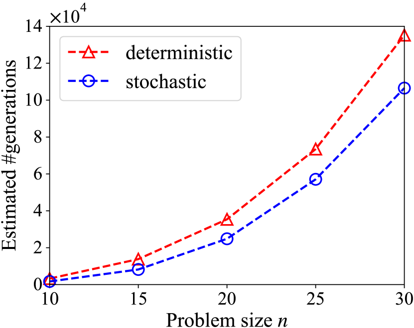
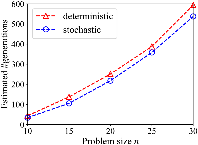
Figure 3: Estimated number of generations of SMS-EMOA and NSGA-II for solving the OneJumpZeroJump  problem with $k=2$. The left subfigure: SMS-EMOA; the right subfigure: NSGA-II.

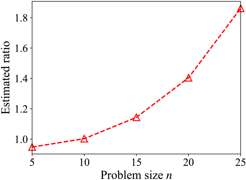
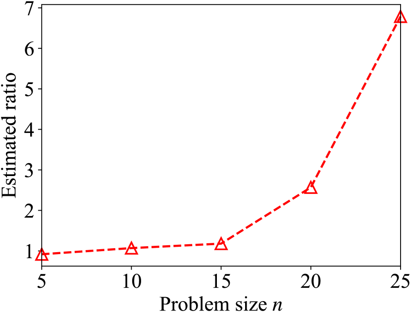
Figure 4: Estimated number of generations of SMS-EMOA and NSGA-II using the deterministic population update divided by that using the stochastic population update for solving the bi-objective RealRoyalRoad  problem. The left subfigure: SMS-EMOA; the right subfigure: NSGA-II.

Table 2: Estimated number of generations of SMS-EMOA and NSGA-II for solving the bi-objective RealRoyalRoad problem.

		$n=5$	$n=10$	$n=15$	$n=20$	$n=25$
SMS-EMOA	Deterministic	43.32	704.22	6572.01	202557.58	10792477.20
	Stochastic	45.71	702.19	5746.85	144221.73	5797042.77
NSGA-II	Deterministic	1.60	26.84	142.56	1858.21	73001.02
	Stochastic	1.81	25.09	120.81	723.53	10757.40

We also examine the performance of SMS-EMOA and NSGA-II solving the bi-objective RealRoyalRoad problem empirically. We set the problem size $n$ from $5$ to $25$ with a step of $5$, and the population size $\mu$ of SMS-EMOA and NSGA-II to $2(2n/5+2)$ and $8(2n/5+1)$, respectively, as suggested in Theorems 3.10 and 4.5. For each $n$, we also run the algorithms 1000 times independently, and report the average number of generations until the Pareto front is found. Since the number of generations of SMS-EMOA/NSGA-II using the deterministic population update is much larger than that using the stochastic population update, we plot the ratio of the average number of generations using these two methods in Figure 4, and also present the detailed average number of generations in Table 2. We can observe that the stochastic population update method can bring a significant acceleration for large $n$.

In addition, it is worth mentioning that using non-dominated sorting, hypervolume indicator and crowding distance to rank solutions also requires computational budget. The stochastic population update method which only needs to compare part of the solutions can make the algorithm even faster.

6 Conclusion

In this paper, we, through rigorous theoretical analysis, question a common practice in the design of MOEAs. Existing well-established MOEAs always update their population in a deterministic manner to select the best solutions. Here we prove that for the well-known SMS-EMOA and NSGA-II, introducing randomness into the population update procedure can significantly decrease the expected running time by enabling the evolutionary search to go along inferior regions close to Pareto optimal regions. We hope our findings can inspire the design of new practical MOEAs, especially those being able to jump out of local optima more easily, which has been recently shown to be a major problem for existing MOEAs li2023moeas .

7 Acknowledgements

We want to thank the anonymous reviewer of IJCAI’23 who suggested us to use the “lucky way” method to prove the upper bound on the expected number of generations of SMS-EMOA with the stochastic population update for solving OneJumpZeroJump, and the other reviewers for their valuable comments.

References

- [1] H. E. Aguirre and K. Tanaka. Insights on properties of multiobjective MNK-landscapes. In Proceedings of the 2004 IEEE Congress on Evolutionary Computation (CEC’04), pages 196–203, Portland, OR, 2004.
- [2] T. Bäck. Evolutionary Algorithms in Theory and Practice: Evolution Strategies, Evolutionary Programming, Genetic Algorithms. Oxford University Press, Oxford, UK, 1996.
- [3] N. Beume, B. Naujoks, and M. Emmerich. SMS-EMOA: Multiobjective selection based on dominated hypervolume. European Journal of Operational Research, 181:1653–1669, 2007.
- [4] C. Bian and C. Qian. Better running time of the non-dominated sorting genetic algorithm II (NSGA-II) by using stochastic tournament selection. In Proceedings of the 17th International Conference on Parallel Problem Solving from Nature (PPSN’22), pages 428–441, Dortmund, Germany, 2022.
- [5] C. Bian, C. Qian, and K. Tang. A general approach to running time analysis of multi-objective evolutionary algorithms. In Proceedings of the 27th International Joint Conference on Artificial Intelligence (IJCAI’18), pages 1405–1411, Stockholm, Sweden, 2018.
- [6] C. Bian, Y. Zhou, M. Li, and C. Qian. Stochastic population update can provably be helpful in multi-objective evolutionary algorithms. In Proceedings of the 32nd International Joint Conference on Artificial Intelligence (IJCAI’23), pages 5513–5521, Macao, SAR, China, 2023.
- [7] D. Brockhoff, T. Friedrich, and F. Neumann. Analyzing hypervolume indicator based algorithms. In Proceedings of the 10th International Conference on Parallel Problem Solving from Nature (PPSN’08), pages 651–660, Dortmund, Germany, 2008.
- [8] S. Cerf, B. Doerr, B. Hebras, Y. Kahane, and S. Wietheger. The first proven performance guarantees for the non-dominated sorting genetic algorithm II (NSGA-II) on a combinatorial optimization problem. In Proceedings of the 32nd International Joint Conference on Artificial Intelligence (IJCAI’23), pages 5522–5530, Macao, SAR, China, 2023.
- [9] C. A. Coello Coello, G. B. Lamont, and D. A. Van Veldhuizen. Evolutionary Algorithms for Solving Multi-objective Problems. Springer, New York, NY, 2007.
- [10] E. Covantes Osuna, W. Gao, F. Neumann, and D. Sudholt. Design and analysis of diversity-based parent selection schemes for speeding up evolutionary multi-objective optimisation. Theoretical Computer Science, 832:123–142, 2020.
- [11] D.-C. Dang, A. Opris, B. Salehi, and D. Sudholt. Analysing the robustness of NSGA-II under noise. In Proceedings of the 25th ACM Conference on Genetic and Evolutionary Computation (GECCO’23), pages 642–651, Lisbon, Portugal, 2023.
- [12] D.-C. Dang, A. Opris, B. Salehi, and D. Sudholt. A proof that using crossover can guarantee exponential speed-ups in evolutionary multi-objective optimisation. In Proceedings of the 37th AAAI Conference on Artificial Intelligence (AAAI’23), pages 12390–12398, Washington, DC, 2023.
- [13] K. Deb. Multi-objective Optimization using Evolutionary Algorithms. Wiley, Chichester, UK, 2001.
- [14] K. Deb and H. Jain. An evolutionary many-objective optimization algorithm using reference-point-based nondominated sorting approach, part I: solving problems with box constraints. IEEE Transactions on Evolutionary Computation, 18(4):577–601, 2014.
- [15] K. Deb, A. Pratap, S. Agarwal, and T. Meyarivan. A fast and elitist multiobjective genetic algorithm: NSGA-II. IEEE Transactions on Evolutionary Computation, 6(2):182–197, 2002.
- [16] M. Dinot, B. Doerr, U. Hennebelle, and S. Will. Runtime analyses of multi-objective evolutionary algorithms in the presence of noise. In Proceedings of the 32nd International Joint Conference on Artificial Intelligence (IJCAI’23), pages 5549–5557, Macao, SAR, China, 2023.
- [17] B. Doerr. Exponential upper bounds for the runtime of randomized search heuristics. Theoretical Computer Science, 851:24–38, 2021.
- [18] B. Doerr, W. Gao, and F. Neumann. Runtime analysis of evolutionary diversity maximization for OneMinMax. In Proceedings of the 18th ACM Conference on Genetic and Evolutionary Computation (GECCO’16), pages 557–564, Denver, CO, 2016.
- [19] B. Doerr, B. Kodric, and M. Voigt. Lower bounds for the runtime of a global multi-objective evolutionary algorithm. In Proceedings of the 2013 IEEE Congress on Evolutionary Computation (CEC’13), pages 432–439, Cancun, Mexico, 2013.
- [20] B. Doerr and F. Neumann, editors. Theory of Evolutionary Computation: Recent Developments in Discrete Optimization. Springer, Cham, Switzerland, 2020.
- [21] B. Doerr and Z. Qu. A first runtime analysis of the NSGA-II on a multimodal problem. IEEE Transactions on Evolutionary Computation, 27(5):1288–1297, 2023.
- [22] B. Doerr and Z. Qu. From understanding the population dynamics of the NSGA-II to the first proven lower bounds. In Proceedings of the 37th AAAI Conference on Artificial Intelligence (AAAI’23), pages 12408–12416, Washington, DC, 2023.
- [23] B. Doerr and Z. Qu. Runtime analysis for the NSGA-II: Provable speed-ups from crossover. In Proceedings of the 37th AAAI Conference on Artificial Intelligence (AAAI’23), pages 12399–12407, Washington, DC, 2023.
- [24] B. Doerr and W. Zheng. Theoretical analyses of multi-objective evolutionary algorithms on multi-modal objectives. In Proceedings of the 35th AAAI Conference on Artificial Intelligence (AAAI’21), pages 12293–12301, Virtual, 2021.
- [25] A. E. Eiben and J. E. Smith. Introduction to Evolutionary Computing. Springer-Verlag, Berlin, Germany, 2015.
- [26] T. Friedrich, N. Hebbinghaus, and F. Neumann. Plateaus can be harder in multi-objective optimization. Theoretical Computer Science, 411(6):854–864, 2010.
- [27] T. Friedrich, C. Horoba, and F. Neumann. Illustration of fairness in evolutionary multi-objective optimization. Theoretical Computer Science, 412(17):1546–1556, 2011.
- [28] O. Giel. Expected runtimes of a simple multi-objective evolutionary algorithm. In Proceedings of the 2003 IEEE Congress on Evolutionary Computation (CEC’03), pages 1918–1925, Canberra, Australia, 2003.
- [29] O. Giel and P. K. Lehre. On the effect of populations in evolutionary multi-objective optimisation. Evolutionary Computation, 18(3):335–356, 2010.
- [30] D. E. Goldberg. Genetic Algorithms in Search, Optimization, and Machine Learning. Addison-Wesley, Boston, MA, 1989.
- [31] J. He and X. Yao. Drift analysis and average time complexity of evolutionary algorithms. Artificial Intelligence, 127(1):57–85, 2001.
- [32] C. Horoba. Analysis of a simple evolutionary algorithm for the multiobjective shortest path problem. In Proceedings of the 10th International Workshop on Foundations of Genetic Algorithms (FOGA’09), pages 113–120, Orlando, FL, 2009.
- [33] Z. Huang, Y. Zhou, C. Luo, and Q. Lin. A runtime analysis of typical decomposition approaches in MOEA/D framework for many-objective optimization problems. In Proceedings of the 30th International Joint Conference on Artificial Intelligence (IJCAI’21), pages 1682–1688, Virtual, 2021.
- [34] M. Laumanns, L. Thiele, and E. Zitzler. Running time analysis of evolutionary algorithms on a simplified multiobjective knapsack problem. Natural Computing, 3:37–51, 2004.
- [35] M. Laumanns, L. Thiele, and E. Zitzler. Running time analysis of multiobjective evolutionary algorithms on pseudo-Boolean functions. IEEE Transactions on Evolutionary Computation, 8(2):170–182, 2004.
- [36] L. H. Lee, C. U. Lee, and Y. P. Tan. A multi-objective genetic algorithm for robust flight scheduling using simulation. European Journal of Operational Research, 177(3):1948–1968, 2007.
- [37] M. Li, X. Han, and X. Chu. MOEAs are stuck in a different area at a time. In Proceedings of the 25th ACM Conference on Genetic and Evolutionary Computation (GECCO’23), pages 303–311, Lisbon, Portugal, 2023.
- [38] Z. Liang, M. Li, and P. K. Lehre. Non-elitist evolutionary multi-objective optimisation: Proof-of-principle results. In Proceedings of the 25th ACM Conference on Genetic and Evolutionary Computation Companion (GECCO’23 Companion), pages 383–386, Lisbon, Portugal, 2023.
- [39] T. Lu, C. Bian, and C. Qian. Towards running time analysis of interactive multi-objective evolutionary algorithms. In Proceedings of the 38th AAAI Conference on Artificial Intelligence (AAAI’24), page in press, Vancouver, Canada, 2024.
- [40] Z. Lu, I. Whalen, V. Boddeti, Y. Dhebar, K. Deb, E. Goodman, and W. Banzhaf. NSGA-Net: neural architecture search using multi-objective genetic algorithm. In Proceedings of the 21th ACM Conference on Genetic and Evolutionary Computation (GECCO’19), pages 419–427, Prague, Czech Republic, 2019.
- [41] H. Markowitz. Portfolio selection. The Journal of Finance, 7(1):77–91, 1952.
- [42] F. Neumann. Expected runtimes of a simple evolutionary algorithm for the multi-objective minimum spanning tree problem. European Journal of Operational Research, 181(3):1620–1629, 2007.
- [43] F. Neumann and M. Theile. How crossover speeds up evolutionary algorithms for the multi-criteria all-pairs-shortest-path problem. In Proceedings of the 11th International Conference on Parallel Problem Solving from Nature (PPSN’10), pages 667–676, Krakow, Poland, 2010.
- [44] A. Q. Nguyen, A. M. Sutton, and F. Neumann. Population size matters: Rigorous runtime results for maximizing the hypervolume indicator. Theoretical Computer Science, 561:24–36, 2015.
- [45] S. Obayashi, S. Takahashi, and I. Fejtek. Transonic wing design by inverse optimization using MOGA. In Proceedings of the 6th Annual Conference of the Computational Fluid Dynamics Society of Canada (CFD’98), Quebec, Canada, 1998.
- [46] G. Pahl and W. Beitz. Engineering Design: A Systematic Approach. Springer-Verlag, London, UK, 1996.
- [47] C. Qian, K. Tang, and Z.-H. Zhou. Selection hyper-heuristics can provably be helpful in evolutionary multi-objective optimization. In Proceedings of the 14th International Conference on Parallel Problem Solving from Nature (PPSN’16), pages 835–846, Edinburgh, Scotland, 2016.
- [48] C. Qian, Y. Yu, and Z.-H. Zhou. An analysis on recombination in multi-objective evolutionary optimization. Artificial Intelligence, 204:99–119, 2013.
- [49] S.-Y. Shin, I.-H. Lee, D. Kim, and B.-T. Zhang. Multiobjective evolutionary optimization of DNA sequences for reliable DNA computing. IEEE Transactions on Evolutionary Computation, 9(2):143–158, 2005.
- [50] S. Wietheger and B. Doerr. A mathematical runtime analysis of the non-dominated sorting genetic algorithm III (NSGA-III). In Proceedings of the 32nd International Joint Conference on Artificial Intelligence (IJCAI’23), pages 5657–5665, Macao, SAR, China, 2023.
- [51] Q. Zhang and H. Li. MOEA/D: A multiobjective evolutionary algorithm based on decomposition. IEEE Transactions on Evolutionary Computation, 11(6):712–731, 2007.
- [52] W. Zheng and B. Doerr. Runtime analysis for the NSGA-II: Proving, quantifying, and explaining the inefficiency for many objectives. IEEE Transactions on Evolutionary Computation, in press.
- [53] W. Zheng and B. Doerr. Better approximation guarantees for the NSGA-II by using the current crowding distance. In Proceedings of the 24th ACM Conference on Genetic and Evolutionary Computation (GECCO’22), pages 611–619, Boston, MA, 2022.
- [54] W. Zheng and B. Doerr. Mathematical runtime analysis for the non-dominated sorting genetic algorithm II (NSGA-II). Artificial Intelligence, 325:104016, 2023.
- [55] W. Zheng and B. Doerr. Runtime analysis of the SMS-EMOA for many-objective optimization. In Proceedings of the 38th AAAI Conference on Artificial Intelligence (AAAI’24), page in press, Vancouver, Canada, 2024.
- [56] A. Zhou, B.-Y. Qu, H. Li, S.-Z. Zhao, P. N. Suganthan, and Q. Zhang. Multiobjective evolutionary algorithms: A survey of the state of the art. Swarm and Evolutionary Computation, 1(1):32–49, 2011.
- [57] Z.-H. Zhou, Y. Yu, and C. Qian. Evolutionary Learning: Advances in Theories and Algorithms. Springer, Singapore, 2019.
- [58] E. Zitzler and S. Künzli. Indicator-based selection in multiobjective search. In Proceedings of the 8th International Conference on Parallel Problem Solving from Nature (PPSN’04), pages 832–842, Birmingham, UK, 2004.
- [59] E. Zitzler, M. Laumanns, and L. Thiele. SPEA2: Improving the strength Pareto evolutionary algorithm. TIK-Report, 103, 2001.
- [60] E. Zitzler and L. Thiele. Multiobjective evolutionary algorithms: A comparative case study and the strength Pareto approach. IEEE Transactions on Evolutionary Computation, 3(4):257–271, 1999.