Explore and Exploit the Diverse Knowledge in Model Zoo
for Domain Generalization

Abstract

The proliferation of pretrained models, as a result of advancements in pretraining techniques, has led to the emergence of a vast zoo of publicly available models. Effectively utilizing these resources to obtain models with robust out-of-distribution generalization capabilities for downstream tasks has become a crucial area of research. Previous research has primarily focused on identifying the most powerful models within the model zoo, neglecting to fully leverage the diverse inductive biases contained within. This paper argues that the knowledge contained in weaker models is valuable and presents a method for leveraging the diversity within the model zoo to improve out-of-distribution generalization capabilities. Specifically, we investigate the behaviors of various pretrained models across different domains of downstream tasks by characterizing the variations in their encoded representations in terms of two dimensions: diversity shift and correlation shift. This characterization enables us to propose a new algorithm for integrating diverse pretrained models, not limited to the strongest models, in order to achieve enhanced out-of-distribution generalization performance. Our proposed method demonstrates state-of-the-art empirical results on a variety of datasets, thus validating the benefits of utilizing diverse knowledge.

1 Introduction

Although remarkable success has been achieved on multiple benchmarks, machine learning models encounter failures in their real-world applications (Volk et al., 2019; Beery et al., 2018b; Dai & Van Gool, 2018). A central cause for such failures has been recognized as the vulnerability to the distribution shifts of the test data (Arjovsky et al., 2019; Gulrajani & Lopez-Paz, 2021). This can occur when test data is collected under new conditions such as different weather (Volk et al., 2019), locations (Beery et al., 2018b), or light conditions (Dai & Van Gool, 2018), resulting in a distribution that differs from the training set.

To address this challenge, the task of domain generalization (DG) has gained significant attention, where models are trained on multiple source domains in order to improve their generalizability to unseen domains (Gulrajani & Lopez-Paz, 2021). Multiple DG algorithms have been proposed from various perspectives. However, this problem is still far from being resolved. For example, Ye et al. (2022) have identified two distinct categories of data distribution shifts, namely diversity shift and correlation shift, and empirically observed that the majority of existing algorithms are only able to surpass the simple empirical risk minimization (ERM) in at most one of the categories.

Exploiting pretrained models (PTMs) has shown to be one of the most promising directions for addressing the challenge of DG tasks (Wiles et al., 2022; Ye et al., 2022). Research has demonstrated that pretraining can provide a significant improvement in performance for DG tasks (Wiles et al., 2022). The growing PTM hubs further bring in great opportunities. With the thriving of pretraining technologies, we now have a huge amount of pretrained models (PTMs) published. For example, Hugging Face Hub (2023) contains over 80K models that vary in data sources, architectures, and pretraining frameworks. Such a zoo of PTMs thus enjoys both high transfer ability and diversity. By selecting optimal PTMs for given DG datasets from a zoo of PTMs, Dong et al. (2022) boosted the state-of-the-art DG performance on some benchmarks for over 14%.

While utilizing PTMs has proven to be a promising approach for domain generalization, it remains unclear how to effectively leverage the diverse inductive biases present in different PTMs. Ensemble methods of PTMs have been explored (Dong et al., 2022; You et al., 2021), however, these methods typically only consider the top-performing models based on performance ranking scores. For example, Dong et al. (2022) proposed a feature selection method on the concatenated features of the top-3 ranked PTMs. However, without incorporating diversity, such ensembles can perform worse than single models. Although some previous studies have examined certain characteristics of different PTMs (Gontijo-Lopes et al., 2022; Idrissi et al., 2022), they are not specified for DG tasks but focus on the in-distribution behavior of the models. This makes it unclear how to effectively utilize these analyses for tackling DG tasks.

To address this challenge, it is crucial to first investigate the compatibility of different PTMs on specific DG tasks and to understand their inductive biases as thoroughly as possible. To achieve this, we propose to profile the shift behaviors of each PTM when conditioned on a given DG task, and then to design an ensemble algorithm that can effectively utilize the profiled shift types. Specifically, similar to the definition presented in (Ye et al., 2022), we interpret the behaviors of PTMs across different domains of downstream tasks by characterizing the variation in their encoded representations from two dimensions, namely feature diversity shift and feature correlation shift. Through this design, we empirically demonstrate that the differences in shift patterns not only exist among datasets but also among different PTMs.

Such profiling provides guidance for utilizing the inductive bias of poorly performed models which have typical shift patterns on one of the dimensions. As these models capture features that induce a specific kind of distribution shift, we can design ensemble algorithms that prevent the classifier from encountering similar failures, thus improving the out-of-distribution (OOD) generalization ability.

To accomplish this, we introduce two key components in our ensemble algorithm: the sample reweight module and the independence penalization module. The sample reweight module utilizes the output of a correlation shift-dominated model to balance the weights of sub-populations, while the independence penalization module requires the main classifier’s output to be independent of features that encounter significant diversity shifts among domains. These ensemble procedures are applied during the training process, introducing no additional computational cost for inference.

We empirically verify the value of such model zoology on image classification benchmarks, with a model zoo that consists of 35 PTMs varying in architecture, pretraining algorithm, and datasets. The results of our empirical analysis demonstrate the effectiveness of our approach in leveraging poor models to enhance performance, as our new algorithm outperforms top model ensembles. We show that the selected models are different across different datasets, which indicates that our method is adaptive to the specific DG tasks.

Our contributions can be summarized as follows.

• We propose a novel methodology for profiling the behavior of pretrained models (PTMs) on a given domain generalization (DG) task by quantifying the distribution shift of the features from two dimensions, namely feature diversity shift and feature correlation shift.

• We introduce a new ensemble algorithm that leverages the insights from the profiled shift types to effectively utilize the diverse inductive bias among different PTMs for DG tasks.

• Through extensive experiments on image classification DG benchmarks, we demonstrate the effectiveness of our proposed approach, which outperforms top-performing PTM ensembles.

This work provides a new perspective on how to effectively leverage the diverse inductive bias of PTMs for domain generalization tasks and highlights the importance of understanding the shift behaviors of models for such tasks.

2 Related Works

Domain generalization.

Numerous domain generalization algorithms have been proposed to alleviate the accuracy degradation caused by distribution shifts via exploiting training domain information  (Arjovsky et al., 2019; Krueger et al., 2021; Li et al., 2018; Bai et al., 2021a; Kuang et al., 2018; Bai et al., 2021b; Cha et al., 2021; Wang et al., 2022; Yi et al., 2023). However, (Gulrajani & Lopez-Paz, 2021) empirically show that recent domain generalization algorithms show no improvement compared with ERM. More fine-grained analyses are further conducted (Ye et al., 2022; Wiles et al., 2022), where distribution shifts are decomposed into multiple categories. Ye et al. (2022) empirically observed that the majority of the algorithms are only able to surpass the simple ERM in at most one kind of distribution shift. Wiles et al. (2022) show that progress has been made over a standard ERM baseline. Though best methods are not consistent over different data shifts, pretraining and augmentations usually offer large gains.

PTMs for domain generalization.

Methods leveraging pretraining models have shown promising improvements in domain generalization performance (Wiles et al., 2022; Li et al., 2022; Arpit et al., 2021; Dong et al., 2022; Wortsman et al., 2022; Rame et al., 2022; Ramé et al., 2022). Among them, ensemble methods combined with PTMs show further advantages. Weight averaging methods combine weights of PTMs of the same architecture over different runs (Rame et al., 2022; Wortsman et al., 2022) or tasks (Ramé et al., 2022). Arpit et al. (2021) ensemble the predictions of moving average models. Recent methods (Li et al., 2022; Dong et al., 2022) further consider the ensemble of models with different architectures to exploit the growing large PTM hubs. Specifically, Li et al. (2022) ensemble predictions of multiple different PTMs via instance-specific attention weights. ZooD (Dong et al., 2022) releases the inference cost by only concatenating the representations of top models selected from a diverse model zoo and further conducts Bayesian feature selection. However, as shown in (Dong et al., 2022), such an ensemble does not always outperform the single model. The diversity in the model zoo has not been fully understood and exploited, which is the focus of this paper.

Understanding PTMs.

The paradigm of PTM reusing triggers the need for understanding the behavior of a PTM on a given downstream task. Recently, studies on the difference in PTM features have been proposed (Gontijo-Lopes et al., 2022; Idrissi et al., 2022), which focus on the in-distribution behavior of models. Gontijo-Lopes et al. (2022) suggest that models under different pretraining techniques learn diverse features. They propose that the correct predictions of high-accuracy models do not dominate those of low-accuracy models, and model ensembles with diverse training methodologies yield the best downstream performance. Idrissi et al. (2022) introduced ImageNet-X, which is a set of human annotations pinpointing failure types for the ImageNet (Russakovsky et al., 2015a) dataset. ImageNet-X labels distinguishing object factors (e.g. pose, color) for each image in the validation set and a random subset. They found that most models when trained, fine-tuned, or evaluated on ImageNet, have the same biases. However, this paper shows different observations on the DG datasets, which will be further discussed in Section 3.3.

3 Model Exploration

To effectively leverage diversity within a model zoo, we need to understand the difference between PTMs conditioned on each specific DG task. To accomplish this, we propose analyzing and describing the changes in PTM feature distributions across downstream domains.

3.1 Feature Diversity and Correlation Shifts

Consider a dataset $\mathcal{D}$ that contains samples collected under multiple domains $\mathcal{E}$, i.e., $\mathcal{D}=\{D_{e}\}_{e\in\mathcal{E}}$. $D_{e}=\left\{x_{i}^{e},y_{i}^{e}\right\}_{i=1}^{n^{e}}$ contains instances of random variables $(X,Y)$ that are i.i.d. sampled from the probability distribution $\mathbb{P}^{e}(\mathcal{X}\times\mathcal{Y})$. Consider a PTM that can be viewed as a feature encoder $\phi:\mathcal{X}\rightarrow\mathcal{Z}_{\phi}$. To understand the behavior of such an encoder between different domains, we are in fact concerned with the difference between the distributions of $(\phi(X),Y)$ on different $\mathbb{P}^{e},\forall e\in\mathcal{E}$. As $\mathbb{P}^{e}(\phi(X),Y)=\mathbb{P}^{e}(Y|\phi(X))\mathbb{P}^{e}(\phi(X))$, the variation of $\mathbb{P}^{e}(\phi(X),Y)$ can be decomposed into the shift of $\mathbb{P}^{e}(\phi(X))$ and the shift of $\mathbb{P}^{e}(Y|\phi(X))$, namely the feature diversity shift and the feature correlation shift.

In this paper, we use the following two metrics for measuring the diversity shift and correlation shift of $\phi:\mathbf{x}\mapsto\mathbf{z}$ between a pair of domains $e,e^{\prime}$, respectively:

$$F_{div}(\phi,e,e^{\prime}) =\frac{1}{2}\int_{\mathcal{S}}|p_{e}(\mathbf{z})-p_{e^{\prime}}(\mathbf{z})|\,\mathrm{d}\mathbf{z},$$

$$F_{cor}(\phi,e,e^{\prime}) =\frac{1}{2}\int_{\mathcal{T}}\tilde{p}_{e,e^{\prime}}(\mathbf{z})\sum_{y\in\mathcal{Y}}|p_{e}(y|\mathbf{z})-p_{e^{\prime}}(y|\mathbf{z})|\,\mathrm{d}\mathbf{z},$$

where $\tilde{p}_{e,e^{\prime}}$ is an geometric average of $p_{e}$ and $p_{e^{\prime}}$. $\mathcal{S}$ and $\mathcal{T}$ are partitions of the image set $Z_{\phi}$ of $\phi$ defined as follows:

$$\mathcal{S}(\phi,e,e^{\prime}) :=\{\mathbf{z}\in\mathcal{Z}_{\phi}|p_{e}(\mathbf{z})\cdot p_{e^{\prime}}(\mathbf{z})=0\},$$

$$\mathcal{T}(\phi,e,e^{\prime}) :=\{\mathbf{z}\in\mathcal{Z}_{\phi}|p_{e}(\mathbf{z})\cdot p_{e^{\prime}}(\mathbf{z})\neq 0\}.$$

Intuitively, $F_{div}$ describes the proportion of values of features $\phi(\mathbf{x})$ not shared between two domains. $F_{cor}$ measures how the correlation between the features and the target label changes between domains. Such definitions are similar to that of diversity shift and correlation shift of datasets in OOD-Bench (Ye et al., 2022). Note that the two metrics in this paper are defined for general feature encoders, not a specific encoder $Z_{2}$ which encodes the latent spurious variable assumed in the data generating process as in (Ye et al., 2022). By specific to that encoder, (Ye et al., 2022) view the two metrics as a characteristic of the dataset itself. In contrast, we focus on the difference between general encoders on a given dataset. That generality requires a new design for the estimation methods of the two metrics than that in (Ye et al., 2022). We further introduce the practical estimation method we proposed in Section 3.2.

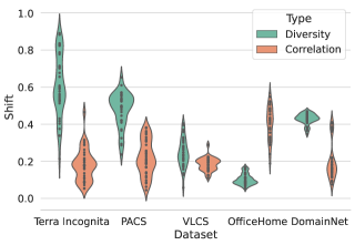
Figure 1: The distribution of feature diversity and correlation shift scores of 35 PTMs on 5 datasets in the DomainBed.

Relation with OOD performance.

For diversity shift, the model’s decision on data from the set $\mathcal{S}$ depends on the classification layer’s extrapolation behavior, which is hard to infer with in-distribution data. For correlation shift, it directly causes the change of prediction precision and results in the gap between in-distribution and out-of-distribution performance. As a result, we would prefer a representation with both low diversity and correlation shifts so that the in-distribution training controls the out-of-distribution error. Note that by splitting the data into $\mathcal{S}$ and $\mathcal{T}$, we leave out the part that is affected by the classification layer’s extrapolation behavior in the correlation shift estimation and the in-domain density shift in the diversity shift estimation. This is the main difference from the scores designed in ZooD.

3.2 Practical Estimation

In this section, we show how the two metrics can be computed practically for general latent features of an arbitrary PTM.

Diversity shift.

Denote $\mathcal{S}_{e}(e^{\prime},\phi):=\{\mathbf{z}\in\mathcal{Z}_{\phi}|p_{e}(\mathbf{z})>0,p_{e^{\prime}}(\mathbf{z})=0\}$, $\mathcal{S}_{e^{\prime}}(e,\phi):=\{\mathbf{z}\in\mathcal{Z}_{\phi}|p_{e}(\mathbf{z})=0,p_{e^{\prime}}(\mathbf{z})>0\}$, $F_{div}(\phi,e,e^{\prime})$ can be written as

$$F_{div}(\phi,e,e^{\prime})=\frac{1}{2}(\mathbb{P}^{e}[\mathcal{S}_{e}(e^{\prime},\phi)]+\mathbb{P}^{e^{\prime}}[\mathcal{S}_{e^{\prime}}(e,\phi)]).$$

We design the following empirical estimation of $\mathbb{P}^{e}[\mathcal{S}_{e}(e^{\prime},\phi)]$:

$$\hat{\mathbb{P}}^{e}[\hat{\mathcal{S}_{e}}(e^{\prime},\phi)]:=\hat{\mathbb{P}}^{e}(\{\mathbf{x}\in D_{e}|\hat{p}_{e^{\prime}}(\mathbf{z})<\epsilon_{e^{\prime}},\mathbf{z}=\phi(\mathbf{x})\}).$$

Intuitively, we estimate the no-overlap set $\mathcal{S}_{e}(e^{\prime},\phi)$ using the estimated probability of the instance in the estimated distribution $\hat{p}_{e^{\prime}}$. When the probability is lower than a given small threshold $\epsilon_{e^{\prime}}$, it is considered as in the set $\mathcal{S}_{e}(e^{\prime},\phi)$. The threshold $\epsilon_{e^{\prime}}$ is estimated by

$$\hat{\mathbb{P}}^{e^{\prime}}(\{\mathbf{x}\in V_{e^{\prime}}|\hat{p}_{e^{\prime}}(\mathbf{z})<\epsilon_{e^{\prime}},\mathbf{z}=\phi(\mathbf{x})\})=0.01.$$

We approximate $p_{e}$ with a Gaussian distribution $\mathcal{N}(\mu_{e},\Sigma_{e})$, and estimate the parameters with empirical statistics on $D_{e}$. In the same way we can get the estimation of $\mathbb{P}^{e^{\prime}}[\mathcal{S}_{e^{\prime}}(e,\phi)]$. The empirical diversity metric is then the average of the two estimations.

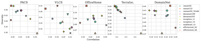
Figure 2: Results of PTMs with different architectures pretrained under the empirical risk minimization framework on ImageNet-1K. Details of these PTMs are provided in Table 5.

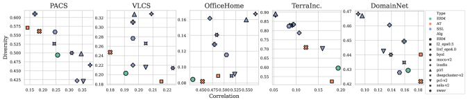
Figure 3: Results comparing ResNet-50s pretrained on ImageNet under different pretraining frameworks. Type denotes different pretraining types, including ERM (empirical risk minimization), AT (adversarial training), and SSL (self supervised learning). Alg denotes the specific pretraining algorithm.

Correlation shift.

For each pair of domain $e,e^{\prime}$. We have the empirical set $\hat{\mathcal{T}}(\phi,e,e^{\prime}):=(D_{e}\setminus\hat{S}_{e}(e^{\prime},\phi))\cup(D_{e^{\prime}}\setminus\hat{S}_{e^{\prime}}(e,\phi))$. Denote $p_{e,e^{\prime}}=\frac{1}{2}(p_{e}+p_{e^{\prime}})$ and

$$\hat{D}_{cor} =\frac{1}{2}\sum_{\mathbf{x}\in\hat{\mathcal{T}}}\hat{p}_{e,e^{\prime}}(\mathbf{x})\sum_{y\in\mathcal{Y}}|\hat{p}_{e}(y|\phi(\mathbf{x}))-\hat{p}_{e^{\prime}}(y|\phi(\mathbf{x}))|.$$

As $D_{e},D_{e^{\prime}}$ are independently sampled, $\hat{p}_{e,e^{\prime}}(\mathbf{x})$ can be estimated by the empirical distribution, i.e., $\hat{p}_{e,e^{\prime}}(\mathbf{x})=1/|D_{e}\cup D_{e}^{\prime}|$. To estimate $\hat{p}_{e}(y|\phi(\mathbf{x}))$, we first get a primary estimation $\tilde{p}_{e}(y|\phi(\mathbf{x}))$ with the following equation, where the coefficient matrices $(\mathbf{M}_{0},\mathbf{M}_{1},\dots,\mathbf{M}_{|\mathcal{Y}|})$ are estimated by minimizing the empirical evidence as in LogME (You et al., 2021), i.e.,

$$\tilde{p}_{e}(y|\phi(\mathbf{x})):=m(\mathbf{M}_{0}\phi(\mathbf{x}),\mathbf{M}_{1}\phi(\mathbf{x}),\dots,\mathbf{M}_{|\mathcal{Y}|}\phi(\mathbf{x})),$$

where $m$ denotes the normalization operator. We then calibrate $\tilde{p}_{e}(y|\phi(\mathbf{x}))$ with the empirical accuracy estimated on $\hat{\mathcal{T}}(\phi,e,e^{\prime})$ to get the final estimation $\hat{p}_{e}(y|\phi(\mathbf{x}))$. More details are provided in Appendix A.1.

3.3 Observations

In this section, we present the results of our empirical analysis on the distribution shifts of PTMs for different DG datasets. We quantify these shifts using the metrics previously described and discuss the various patterns observed.

We conduct experiments on five domain generalization benchmarks: PACS (Li et al., 2017), VLCS (Fang et al., 2013), Office-Home (Venkateswara et al., 2017), TerraIncognita (Beery et al., 2018a), DomainNet (Peng et al., 2019). According to (Ye et al., 2022), PACS, OfficeHome, and TerraIncognita all only encounter diversity shifts, while DomainNet shows both diversity and correlation shifts. We adopt the model zoo constructed in (Dong et al., 2022), which consists of 35 PTMs with diverse architectures, pre-training methods, and pre-training datasets. The two shift scores for each model are the average of the two metrics in Section 3.1 computed on each pair of domains in the dataset. More details are provided in Appendix A.2.

The primary findings in this section are as follows.

• Within a specific DG dataset, the shift patterns of PTMs exhibit substantial diversity.

• The architectural diversity contributes to distinct shift patterns, and their interrelationships tend to maintain consistency across datasets.

• The influence of pretraining frameworks on shift behavior is noteworthy. Particularly, self-supervised learning leads to relatively higher feature diversity shifts.

• An increase in the size of the pretraining data results in a decrease in the feature correlation shift.

We introduce those findings in detail in the following paragraphs.

Different shift patterns of PTMs on the datasets.

As shown in (Ye et al., 2022), different datasets exhibit different trends of shifts. A natural question is how the distribution shift of data interacts with the shift in the feature space of a PTM. The observations in this section show that the shift patterns of PTMs can have a great variety within a given DG dataset. Specifically, we compute the average shift metric scores between domain pairs on each dataset. The results are shown in Figure 1. On Terra Incognita, the diversity shift of models varies from 0.21 to 0.89. Notably, some PTMs encounter significant correlation shifts on Terra Incognita, which is different from the dataset correlation shift shown in (Ye et al., 2022).

We further compare the results within the following 3 groups of models to show the effect of architectures, training frameworks, and datasets on shift behavior. The details of the 3 groups are introduced in Appendix A.2.

Architectures.

We compare models with different architectures but pre-trained with the same framework on the same dataset. As shown in Figure 2, when comparing PTMs pretrained under the ERM framework on ImageNet-1K (Russakovsky et al., 2015a), we found that the variation of architectures resulted in a wide range of shift patterns. It can be observed that across different datasets, ResNet-152 generally exhibits a larger diversity shift compared to ResNet-50, and a smaller correlation shift. Additionally, after fine-tuning, ResNet-152 achieves higher OOD accuracy than ResNet-50. These findings suggest an interesting observation that while ResNet-152 captures domain-specific features, they do not result in a geometric skew (Nagarajan et al., 2021).

Pretraining frameworks.

To show the effect of pretraining frameworks, we compare models with a fixed architecture but trained with different optimization objectives on the same dataset. Figure 3 shows the results comparing ResNet-50s pretrained on ImageNet under different frameworks, i.e., ERM, self-supervised learning (SSL), and adversarial training (AT) (Madry et al., 2018). We can find models pretrained using SSL methods exhibit overall higher diversity shifts. This is not unexpected, as SSL methods tend to learn features that maximally preserve the original information of the raw input, including the domain-specific part. For example, generative-based SSL such as the Masked autoencoder (He et al., 2021) learns to reconstruct images with only a small fraction of the pixels. Additionally, contrastive learning methods have been observed to suffer from the negative transfer phenomenon (Liu et al., 2022), where the learned features perform poorly on downstream tasks. Furthermore, the use of cosine similarity in contrastive learning has been noted to result in overly complex feature maps (Hu et al., 2022a), which can negatively impact out-of-distribution generalization. Among SSL methods, PIRL (Misra & van der Maaten, 2020) and InsDis (Wu et al., 2018) usually have the most significant diversity shifts and worse OOD performance on these datasets (Dong et al., 2022).

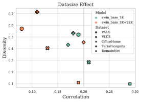
Figure 4: Results of Swin transformers (Liu et al., 2021) pretrained on ImageNet-1K and both ImageNet-1K and ImageNet-22K on 5 datasets.

Datasets.

To demonstrate the impact of dataset size on the distribution shifts of PTMs, we compare the performance of Swin transformers (Liu et al., 2021) pretrained on ImageNet-1K and both ImageNet-1K and ImageNet-22K (Russakovsky et al., 2015b), as shown in Figure 4. It indicates that the use of larger pretraining data results in a significant decrease in correlation shift, which may be attributed to the increased complexity of the supervised pretraining tasks.

4 Model Zoo Exploitation

In this section, we demonstrate how the characteristic of diversity in models can be employed to enhance the domain generalization performance of strong models. In the previous section, we established that models exhibit two distinct types of shift patterns. Our observations indicate that some PTMs are dominated by one type of shift, for example, PIRL on TerraIncognita. This insight inspires the design of an ensemble algorithm that addresses the two dimensions of feature shifts. By leveraging two auxiliary models that are dominated by the two shifts respectively, we design corresponding algorithms to resolve the specific shifts.

Table 1: Comparison of test domain accuracy between our method and SOTA OOD methods. The results of SWAD are from (Cha et al., 2021), and results denoted with ${\dagger}$ are from (Gulrajani & Lopez-Paz, 2021). The results of three versions of ZooD are from (Dong et al., 2022) (denoted with $*$). Our results are average of three trials.

Method	PACS	VLCS	OfficeHome	TerraInc.	DomainNet	Avg
ERM†	85.5	77.5	66.5	46.1	40.9	63.3
IRM†	83.5	78.6	64.3	47.6	33.9	61.6
GroupDRO†	84.4	76.7	66.0	43.2	33.3	60.7
I-Mixup†	84.6	77.4	68.1	47.9	39.2	63.4
MMD†	84.7	77.5	66.4	42.2	23.4	58.8
SagNet†	86.3	77.8	68.1	48.6	40.3	64.2
ARM†	85.1	77.6	64.8	45.5	35.5	61.7
VREx†	84.9	78.3	66.4	46.4	33.6	61.9
RSC†	85.2	77.1	65.5	46.6	38.9	62.7
SWAD	88.1	79.1	70.6	50.0	46.5	66.9
ZooD
Single∗	96.0	79.5	84.6	37.3	48.2	69.1
Ensemble∗	95.5	80.1	85.0	38.2	50.5	69.9
F. Selection∗	96.3	80.6	85.1	42.3	50.6	71.0
Ours
Single + Rew	96.3	81.2	84.0	52.0	48.2	72.3
+ HSIC	96.7	81.5	85.2	52.3	49.2	72.8
+ Both	96.7	81.4	85.3	53.0	49.2	73.1

4.1 Diversity Ensemble Method

To prevent potential failure caused by the diversity shift, we utilize the auxiliary model which encodes features that encounter significant diversity shifts. We propose to require the prediction of the main model to be independent of those features thus mitigating the effect of diversity shift on the predictor. To constraint the independence, we adopt a differentiable independence measure, the Hilbert-Schmidt independence criterion (HSIC) (Gretton et al., 2007). The idea of using HSIC is inspired by the algorithm proposed in (Bahng et al., 2020), where HSIC is used for penalizing the dependency between the predicts of the main model and multiple biased models.

Formally, denote $Z_{l}=l_{m}\circ f_{M}(X)$, where $l_{m}:\mathcal{Z}_{M}\rightarrow\mathcal{Z}_{l}$ is the classifier on the top of the main model $f_{M}:\mathcal{X}\rightarrow\mathcal{Z}_{M}$. Denote $Z_{d}=f_{d}(X)$, where $f_{d}:\mathcal{X}\rightarrow\mathcal{Z}_{d}$ is the diversity auxiliary model. Our target is then to constrain the dependency between $Z_{l}$ and $Z_{d}$. Denote $k$ as a kernel function on $\mathcal{Z}_{d}\times\mathcal{Z}_{d}$, $l$ as a kernel function on $\mathcal{Z}_{l}\times\mathcal{Z}_{l}$. The HSIC statistic between the main model $f_{M}$ and the auxiliary model $f_{d}$ is defined as follows:

$$\textrm{HSIC}(f_{M},f_{d}):= \mathbb{E}\left[k\left(Z_{d},Z_{d}^{\prime}\right)l\left(Z_{l},Z_{l}^{\prime}\right)\right]+$$

$$\quad\mathbb{E}\left[k\left(Z_{d},Z_{d}^{\prime}\right)\right]\mathbb{E}\left[l\left(Z_{l},Z_{l}^{\prime}\right)\right]$$

$$\;\;-2\mathbb{E}\left[\mathbb{E}_{Z_{d}^{\prime}}\left[k\left(Z_{d},Z_{d}^{\prime}\right)\right]\mathbb{E}_{Z_{l}^{\prime}}\left[l\left(Z_{l},Z_{l}^{\prime}\right)\right]\right].$$

Instead of the unbiased estimator in (Bahng et al., 2020), we used the biased empirical estimate $\mathrm{HSIC}_{b}$ (Gretton et al., 2007):

$$\textrm{HSIC}_{b}(f_{M},f_{d}):=\frac{1}{m^{2}}\operatorname{trace}(\mathbf{KHLH}),$$

where we suppose the sample size is $m$, $\mathbf{K}$ denotes the $m\times m$ matrix with entries $k_{ij}:=k(f_{d}(x_{i}),f_{d}(x_{j}))$, $\mathbf{L}$ denotes the $m\times m$ matrix with entries $l_{ij}:=l(l_{m}\circ f_{M}(x_{i}),l_{m}\circ f_{M}(x_{j}))$. $\mathbf{H}=\mathbf{I}-\frac{1}{m}\mathbf{1}\mathbf{1}^{T}$, where $\mathbf{1}$ is an $m\times 1$ vector of ones.

The final training objective of the main model writes as follows:

$$\mathcal{L}(f_{M}):=\min_{f_{M}}\mathbb{E}_{X,Y\sim\mathbb{P}_{\mathcal{D}}} [\mathcal{L}_{c}(Y,f_{M}(X))$$

$$+\lambda\mathrm{HSIC}_{d}(f_{M},f_{d})].$$

In our implementation, we use the Gaussian kernel $l(z,z^{\prime})=\exp(-\gamma_{1}\lVert z-z^{\prime}\rVert^{2})$, $k(z,z^{\prime})=\exp(-\gamma_{2}\lVert z-z^{\prime}\rVert^{2})$. To mitigate the effect of the dimension, we rescale $\gamma_{1}$ and $\gamma_{2}$ by dividing by the dimension of the representation $z$ in the calculation. Following methods in invariant learning literature (Chen et al., 2022), we introduce an additional hyperparameter $N_{\textrm{warm-up}}$ which controls the number of warm-up steps before the HSIC penalty is added to the loss.

Table 2: Main and auxiliary models. HSIC aux. denotes the auxiliary models that are dominated by the diversity shift and adopted for computing the HSIC constraint. Rew. aux. denotes the auxiliary models that are dominated by the correlation shift. The metric values are averaged over each pair of domains in the dataset. Details of the model configuration are provided in Appendix B.1.

Datasets	PACS	VLCS	OfficeHome	TerraInc.	DomainNet
Main model	CLIP-ViT	CLIP-ViT	Swin-B-22	Swin-B-22	ResNext-101
$F_{div}$	0.37	0.36	0.11	0.71	0.35
$F_{cor}$	0.05	0.11	0.19	0.11	0.41
HSIC aux.	ResNet50-ss	ResNet50-InsDis	ResNet50-InsDis	ResNet50-PIRL	ViT-B
$F_{div}$	0.65	0.33	0.17	0.89	0.47
$F_{cor}$	0.10	0.21	0.57	0.05	0.22
Rew. aux.	BEiT-base	BEiT-base	deepcluster-v2	inception-v3	ResNet50-sws
$F_{div}$	0.33	0.06	0.09	0.21	0.45
$F_{cor}$	0.38	0.29	0.52	0.47	0.40

4.2 Correlation Ensemble Method

To prevent potential failure caused by the correlation shift, we adopt the auxiliary model which encodes features that encounter significant correlation shifts. In this module, we reweight training instances to weaken the correlation between the features and the target labels. By that, we avoid the predictor from skewing to that unstable correlation across domains.

Specifically, denote the auxiliary model as $f_{c}$ and its uncertainty output for instance $\mathbf{x}$ as $\mathbf{p}_{c}(\mathbf{x})$. We follow the classical strategy which has been proven effective in the debias literature (Xiong et al., 2021) to reweight the instance loss with

$$w_{c}(\mathbf{x},y)=p(y)/p_{c}(\mathbf{x})_{y},$$

where $p_{c}(\mathbf{x})_{y}$ is the $y$-th component of $\mathbf{p}_{c}(\mathbf{x})$. During training steps, the weights in each batch are smoothed with a hyperparameter $T$ and normalized (Yi et al., 2021). The loss on a batch $|\mathcal{B}|$ is then

$$\mathcal{L}_{\mathcal{B}}(f_{M}):=\frac{1}{|\mathcal{B}|}\sum_{(\mathbf{x},y)\in\mathcal{D}}m(\frac{p(y)}{p_{c}(\mathbf{x})_{y}\cdot T})\mathcal{L}_{c}(y,f_{M}(\mathbf{x})),$$

where $m$ denotes the normalization operation over samples in $\mathcal{B}$. We introduce an additional hyperparameter $N_{\textrm{anneal}}$ which controls the number of annealing steps where $T$ is infinitely large, i.e., before the adjusted weights are attached to the samples.

5 Experiments

We conduct experiments on domain generalization benchmarks to evaluate the effectiveness of our proposed zoo exploiting method. Our results demonstrate that it consistently outperforms single top models and improves the performance of top model ensembles, highlighting the benefits of exploiting model diversity. Additionally, we analyze the correlation between OOD accuracy and the feature diversity and correlation shifts of the fine-tuned classifiers.

5.1 Experiment Settings

Datasets.

We conduct experiments on five domain generalization benchmarks: PACS (Li et al., 2017), VLCS (Fang et al., 2013), OfficeHome (Venkateswara et al., 2017) , TerraIncognita (Beery et al., 2018a), and DomainNet (Peng et al., 2019). During training on each dataset, one of the domains is chosen as the target domain and the remaining are the training domains, where 20% samples are used for validation and model selection. The final test accuracy on the dataset is the mean of the test results on each target domain.

Baselines.

We compare the proposed algorithm with previous SOTA OOD methods and three versions of ZooD, including 1) Single: fine-tune the top-1 model ranked by ZooD; 2) Ensemble: fine-tune an ensemble of the top-K models; 3) F. Selection: fine-tune an ensemble of the top-K models with feature selection, which is the expected result using ZooD. Our algorithm also has three versions. 1) Single+Rew: fine-tune the top-1 model ranked by ZooD with reweight auxiliary; 2) Single+HSIC: fine-tune the top-1 model with HSIC auxiliary; 3) Single+Both: fine-tune the top-1 model with both kinds of auxiliary.

Configurations.

We follow the setting of ZooD to construct a model zoo consisting of 35 PTMs. As discussed in Section 3.3, these models vary in architectures, pretraining methods, and datasets. For auxiliary models, we select models that are extreme at one shift metric. For the main model, we use the Top-1 model ranked by ZooD. The detailed statistics of selected auxiliary models and the main models are shown in Table 2. We use a 3-layer MLP as the prediction head on the top of the main model and fine-tune it on the downstream tasks. Following ZooD, we adopt the leave-one-domain-out cross-validation setup in DomainBed for hyper-parameter selection and run 3 trials. More details on the experimental setup are in Appendix B.1.

Table 3: Results on the ensemble of Top-3 models. Results denoted with $*$ are from (Dong et al., 2022).

Datasets	OfficeHome	DomainNet
Ensemble∗	85.0	50.5
F. Selection∗	85.1	50.6
Ensemble+Rew	85.1	50.6
+HSIC	86.0	51.4

Table 4: Shift scores of the last layer representation of main predictors. ERM, HSIC, Rew. and Two denote the scores for the logits of the main predictor.

	Datasets	VLCS	TerraInc.
	Model	CLIP-ViT	Swin-B-22
	Test Env.	1	0
ERM	$F_{div}$	0.11	0.34
	$F_{cor}$	0.06	0.16
HSIC	$F_{div}$	0.095	0.27
	$F_{cor}$	0.041	0.17
Rew.	$F_{div}$	0.101	0.33
	$F_{cor}$	0.054	0.15
Two	$F_{div}$	0.098	0.28
	$F_{cor}$	0.050	0.16

5.2 Experiment Results

Table 1 presents the main results of our proposed methods on the five datasets of the DomainBed benchmark. The results indicate that the incorporation of the independence penalization module and the combination of reweight and independence penalization modules consistently improve the performance of the single top model. On average, the combination of both methods (Single+Both) results in an approximate 6% improvement in accuracy. Notably, on the PACS, VLCS, and TerraIncognita datasets, our proposed methods even outperform the F. Selection method. This observation highlights the potential of utilizing model inductive bias to leverage weak models in boosting performance, rather than relying solely on strong models.

On the OfficeHome and DomainNet datasets, the proposed methods do not show significant improvements over top-3 ensembles (the Ensemble version of ZooD). To further investigate this, we also conducted experiments using our methods on top-3 ensembles. The results, presented in Table 3, reveal that compared to the F. Selection method, the incorporation of the independence penalization module can significantly enhance the overall accuracy.

It is worth noting that, unlike the independence penalization module, the improvements brought by the reweight module are only significant on the VLCS and TerraIncognita datasets. For the PACS dataset, this may be attributed to the fact that the $F_{cor}$ of the main model is already non-significant, as reported in Table 2. For the OfficeHome and DomainNet datasets, this may be due to the limited effectiveness of the reweighting strategy when the number of classes is large (65 and 345). Previous literature has only validated its success on tasks with a number of classes lower than 10 (Xiong et al., 2021).

To further interpret the results, we analyze the shift pattern of the main predictor. Table 4 shows the scores comparison of the last layer features (logits) of the main predictor. The results are obtained using the following hyperparameter set: $\lambda=100,N_{\textrm{warm-up}}=500,\gamma_{1}=0.5,\gamma_{2}=0.25$, $T=1,N_{\textrm{anneal}}=2000$. As expected, compared to the results obtained using ERM, HSIC, and Rew. lead to a decrease in $F_{div}$ and $F_{cor}$, respectively. The results obtained using both modules show a compromise between the two modules. It is worth noting that the use of HSIC on the VLCS dataset leads to a significant decrease in $F_{cor}$, which can explain the result in Table 1 where incorporating the reweight module in Two does not further improve the results of HSIC.

6 Conclusion

In this work, we have presented a novel approach for utilizing the diverse knowledge present in a model zoo for domain generalization tasks. The main takeaway findings of this study are two-fold. Firstly, it emphasizes that even the most powerful models have the potential for further enhancements in downstream DG tasks. Secondly, it illustrates that the enhancements do not solely come from powerful models, but rather from a combination of models with diverse characteristics, a weak model can also contribute to the enhancement of an already strong model. This highlights the importance of maintaining a diverse zoo of pretrained models for the community. It is worth emphasizing that our proposed profiling method is general and can be applied to other tasks and domains, making it an interesting avenue for further research. Overall, this work provides a new perspective on how to better utilize the diverse knowledge in a model zoo and opens up new possibilities for improving performance on out-of-distribution tasks.

Appendix A Shift metrics

A.1 Practical Estimation

In this section, we show how the two metrics can be computed practically for general latent features of an arbitrary PTM.

Notations.

Consider a dataset $\mathcal{D}$ that contains samples collected under multiple domains $\mathcal{E}$, i.e., $\mathcal{D}=\{D_{e}\}_{e\in\mathcal{E}}$. $D_{e}=\left\{x_{i}^{e},y_{i}^{e}\right\}_{i=1}^{n^{e}}$ contains instances of random variables $(X,Y)$ that are i.i.d. sampled from the probability distribution $\mathbb{P}^{e}(\mathcal{X}\times\mathcal{Y})$. A PTM is denoted as a feature encoder $\phi:\mathcal{X}\rightarrow\mathcal{Z}_{\phi}$. Suppose the dimension of $\phi(x)$ is $d$. The feature matrix on the domain $D_{e}$ is denoted as

$$\Phi_{e}:=\big{(}\phi(x^{e}_{1}),\phi(x^{e}_{i2}),\dots,\phi(x^{e}_{n^{e}})\big{)}^{\top}\in\mathbb{R}^{n^{e}\times d}.$$

Diversity shift.

Denote $\mathcal{S}_{e}(e^{\prime},\phi):=\{\mathbf{z}\in\mathcal{Z}_{\phi}|p_{e}(\mathbf{z})>0,p_{e^{\prime}}(\mathbf{z})=0\}$, $\mathcal{S}_{e^{\prime}}(e,\phi):=\{\mathbf{z}\in\mathcal{Z}_{\phi}|p_{e}(\mathbf{z})=0,p_{e^{\prime}}(\mathbf{z})>0\}$, $F_{div}(\phi,e,e^{\prime})$ can be written as

$$F_{div}(\phi,e,e^{\prime})=\frac{1}{2}(\mathbb{P}^{e}[\mathcal{S}_{e}(e^{\prime},\phi)]+\mathbb{P}^{e^{\prime}}[\mathcal{S}_{e^{\prime}}(e,\phi)]).$$

We design the following empirical estimation of $\mathbb{P}^{e}[\mathcal{S}_{e}(e^{\prime},\phi)]$:

$$\hat{\mathbb{P}}^{e}[\hat{\mathcal{S}_{e}}(e^{\prime},\phi)]:=\hat{\mathbb{P}}^{e}(\{\mathbf{x}\in D_{e}|\hat{p}_{e^{\prime}}(\mathbf{z})<\epsilon_{e^{\prime}},\mathbf{z}=\phi(\mathbf{x})\}).$$

Intuitively, we estimate the no-overlap set $\mathcal{S}_{e}(e^{\prime},\phi)$ using the estimated probability of the instance in the estimated distribution $\hat{p}_{e^{\prime}}$. When the probability is lower than a given small threshold $\epsilon_{e^{\prime}}$, it is considered as in the set $\mathcal{S}_{e}(e^{\prime},\phi)$. The threshold $\epsilon_{e^{\prime}}$ is estimated by

$$\hat{\mathbb{P}}^{e^{\prime}}(\{\mathbf{x}\in V_{e^{\prime}}|\hat{p}_{e^{\prime}}(\mathbf{z})<\epsilon_{e^{\prime}},\mathbf{z}=\phi(\mathbf{x})\})=0.01.$$

For each $e\in\mathcal{E}$, we approximate $p_{e}$ with a Gaussian distribution $\mathcal{N}(\mu_{e},\Sigma_{e})$, and estimate the parameters with empirical statistics on $D_{e}$. Specifically,

$$\hat{\mu}_{e}=\frac{1}{n^{e}}\Phi_{e}^{\top}\mathbbm{1}_{n^{e}}\quad\hat{\Sigma}_{e}=\frac{1}{n^{e}}(\Phi_{e}-\mathbbm{1}_{n^{e}}\hat{\mu}_{\phi}^{\top})^{\top}(\Phi_{e}-\mathbbm{1}_{n^{e}}\hat{\mu}_{\phi}^{\top}),$$

Given the estimated distribution $\mathcal{N}(\hat{\mu}_{e},\hat{\Sigma}_{e})$, the probability density at a given point $\mathbf{z}\in\mathcal{Z}_{\phi}$ is computed as

$$\hat{p}_{e}(\mathbf{z})=\hat{p}_{e}(\mathbf{z}|\hat{\mu}_{e},\hat{\Sigma}_{e})=\sqrt{\frac{1}{(2\pi)^{d}|\hat{\Sigma}_{e}|}}\exp\left(-\frac{1}{2}(\mathbf{z}-\hat{\mu}_{e})^{\top}\hat{\Sigma}_{e}^{-1}(\mathbf{z}-\hat{\mu}_{e})\right).$$

Denote $C_{e}:=(2\pi)^{-d/2}|\hat{\Sigma}_{e}|^{1/2}$, $\hat{d}_{e}(\mathbf{z}):=(\mathbf{z}-\hat{\mu}_{e})^{\top}\hat{\Sigma}_{e}^{-1}(\mathbf{z}-\hat{\mu}_{e})$, we have $\hat{p}_{e}(\mathbf{z})=C_{e}\exp(-\frac{1}{2}\hat{d}_{e}(\mathbf{z}))$. As $C_{e}$ is constant for any $\mathbf{z}$, and the exponential function is monotonic, we can empirically estimate $\mathbb{P}^{e}[\mathcal{S}_{e}(e^{\prime},\phi)]$ using $\hat{d}_{e^{\prime}}$ instead as follows:

$$\hat{\mathbb{P}}^{e}[\hat{\mathcal{S}_{e}}(e^{\prime},\phi)]:=\hat{\mathbb{P}}^{e}(\{\mathbf{x}\in D_{e}|\hat{d}_{e^{\prime}}(\mathbf{z})>\epsilon_{e^{\prime}},\mathbf{z}=\phi(\mathbf{x})\}),$$

where $\epsilon_{e^{\prime}}$ satisfies

$$\hat{\mathbb{P}}^{e^{\prime}}(\{\mathbf{x}\in V_{e^{\prime}}|\hat{d}_{e^{\prime}}(\mathbf{z})>\epsilon_{e^{\prime}},\mathbf{z}=\phi(\mathbf{x})\})=0.01.$$

Note that it connects to the common practice in OOD detection methods where the Mahalanobis distance is estimated (Lee et al., 2018).

The estimation of $\mathbb{P}^{e^{\prime}}[\mathcal{S}_{e^{\prime}}(e,\phi)]$ is defined in the same way. The empirical diversity metric is then the average of the two estimations, i.e.,

$$\hat{F}_{div}(\phi,e,e^{\prime})=\frac{1}{2}\left(\hat{\mathbb{P}}^{e}[\hat{\mathcal{S}}_{e}(e^{\prime},\phi)]+\hat{\mathbb{P}}^{e^{\prime}}[\hat{\mathcal{S}}_{e^{\prime}}(e,\phi)]\right).$$

Correlation shift.

For each pair of domain $e,e^{\prime}$. We have the empirical set $\hat{\mathcal{T}}(\phi,e,e^{\prime}):=(D_{e}\setminus\hat{S}_{e}(e^{\prime},\phi))\cup(D_{e^{\prime}}\setminus\hat{S}_{e^{\prime}}(e,\phi))$. Denote $p_{e,e^{\prime}}=\frac{1}{2}(p_{e}+p_{e^{\prime}})$ and

$$\hat{D}_{cor} =\frac{1}{2}\sum_{\mathbf{x}\in\hat{\mathcal{T}}}\hat{p}_{e,e^{\prime}}(\mathbf{x})\sum_{y\in\mathcal{Y}}|\hat{p}_{e}(y|\phi(\mathbf{x}))-\hat{p}_{e^{\prime}}(y|\phi(\mathbf{x}))|.$$

As $D_{e},D_{e^{\prime}}$ are independently sampled, $\hat{p}_{e,e^{\prime}}(\mathbf{x})$ can be estimated by the empirical distribution, i.e., $\hat{p}_{e,e^{\prime}}(\mathbf{x})=1/|D_{e}\cup D_{e}^{\prime}|$. To estimate $\hat{p}_{e}(y|\phi(\mathbf{x}))$, we first get a primary estimation $\tilde{p}_{e}(y|\phi(\mathbf{x}))$ with the following equation:

$$\tilde{p}_{e}(\mathbf{y}|\phi(\mathbf{x})):=m(\mathbf{M}_{0}\phi(\mathbf{x}),\mathbf{M}_{1}\phi(\mathbf{x}),\dots,\mathbf{M}_{|\mathcal{Y}|}\phi(\mathbf{x})),$$ (1)

where $m$ denotes the normalization operator. The coefficient matrices $(\mathbf{M}_{0},\mathbf{M}_{1},\dots,\mathbf{M}_{|\mathcal{Y}|})$ are estimated by minimizing the empirical evidence on $D_{e}$ as in LogME (You et al., 2021). Specifically, denote $K:=|\mathcal{Y}|$, $\mathbf{y}\in\mathbb{R}^{K}$ is the one-hot label vector . Denote $y_{i}$ as the $i$-th component. We adopt the following linear model assumption:

$$y_{i}=\mathbf{w}_{i}^{\top}\phi(x)+\epsilon,\quad\mathbf{w}_{i}\in\mathbb{R}^{d},\,\,\epsilon\in\mathbb{R},$$

where $\epsilon$ is the Gaussian noise variable with variance $\beta^{-1}$. As we assume that the prior distribution of weights $\mathbf{w}_{i}$ is an isotropic Gaussian distribution with zero mean and parameterized by $\alpha$, i.e.

$$\mathbf{w}_{i}\sim\mathcal{N}(\mathbf{0},\alpha^{-1}\mathbb{I}_{d}),$$

and the conditional distribution of $y_{i}$ given $\phi(x)$ is

$$y_{i}\big{|}\phi(x),\mathbf{w}_{i}\sim\mathcal{N}(\mathbf{w}_{i}^{\top}\phi(x),\beta^{-1}),$$

then according to the definition of evidence,

$$p(y_{i}|\phi(x),\alpha,\beta)=\int_{\mathbf{w}_{i}\in\mathbb{R}^{d}}p(\mathbf{w}_{i}|\alpha)p(y_{i}|\phi(x),\mathbf{w}_{i},\beta)d\mathbf{w}_{i}.$$

Denote $\Phi_{e}\in\mathbb{R}^{n_{e}\times d}$ as the feature matrix of all training samples in the environment $e$, and $\mathbf{y}_{i}^{e}\in\mathbb{R}^{n_{e}}$ as the label vector composed by $y_{i}$. Denote $A=\alpha I+\beta\Phi_{e}^{\top}\Phi_{e},m=\beta A^{-1}\Phi_{e}^{\top}\mathbf{y}_{i}^{e}$, we have the following log-likelihood:

$$\mathcal{L}(\alpha,\beta) =\log p(\mathbf{y}_{i}^{e}|\Phi_{e},\alpha,\beta)$$

$$=\frac{n_{e}}{2}\log\beta+\frac{d}{2}\log\alpha-\frac{n_{e}}{2}\log 2\pi$$

$$-\frac{\beta}{2}\|\Phi_{e}m-\mathbf{y}_{i}^{e}\|_{2}^{2}-\frac{\alpha}{2}m^{\top}m-\frac{1}{2}\log|A|.$$

Solve $(\alpha^{*},\beta^{*})=\arg\max_{\alpha,\beta}\mathcal{L}(\alpha,\beta)$ by using the same iterative approach as in  (You et al., 2021), we can get an estimate of $\mathbf{w}_{i}$:

$$\hat{\mathbf{w}}_{i}=\beta^{*}(\alpha^{*}I+\beta^{*}\Phi_{e}^{\top}\Phi_{e})^{-1}\Phi_{e}^{\top}\mathbf{y}_{i}^{e}.$$

Substituting the above estimate into the formula 1, we get the estimate $\tilde{p}_{e}(y|\phi(\mathbf{x}))$. Alternatively, we can also consider directly using square loss for classifying the features and estimating the conditional probability (Hu et al., 2022b). We then calibrate $\tilde{p}_{e}(y|\phi(\mathbf{x}))$ with the empirical accuracy estimated on $\hat{\mathcal{T}}(\phi,e,e^{\prime})$ to get the final estimation $\hat{p}_{e}(y|\phi(\mathbf{x}))$. Specifically, denote $\mathcal{B}_{0},\mathcal{B}_{1},\dots,\mathcal{B}_{b}$ as $b$ average sized blocks in $[0,1]$. We define

$$\mathcal{B}_{i}(\phi,e,y)=\{(\mathbf{x},y)\in D_{e}\cap\hat{T}(\phi,e,e^{\prime})|\tilde{p}_{e}(y|\phi(\mathbf{x}))\in\mathcal{B}_{i}\}.$$

We then estimate $\hat{p}_{e}(y|\phi(\mathbf{x}))$ for $\mathbf{x}\in\mathcal{B}_{i}(\phi,e,y)$ as follows:

$$\hat{p}_{e}(y|\phi(\mathbf{x})):=\frac{|\{(\mathbf{x},y_{x})\in\mathcal{B}_{i}(\phi,e,y)|y_{x}=y\}|}{|\mathcal{B}_{i}(\phi,e,y)|}.$$

The final $\hat{D}_{cor}$ is then computed with the estimated $\hat{p}_{e}(y|\phi(\mathbf{x}))$ and $\hat{p}_{e^{\prime}}(y|\phi(\mathbf{x}))$.

Table 5: Details of the model zoo proposed in (Dong et al., 2022). The first column corresponds to the numbers we have used for subsequent tables. The rest of the table describes architectures, pre-training datasets, and pre-training algorithms as well as the group and source of each model.

Number Architecture Dataset Algorithm Group Source 1 ResNet-50 ImageNet-1K ERM Group 1 Paszke et al. (2019) 2 ResNet-152 ImageNet-1K ERM Group 1 Paszke et al. (2019) 3 ResNeXt-50 ImageNet-1K ERM Group 1 Paszke et al. (2019) 4 DenseNet-169 ImageNet-1K ERM Group 1 Paszke et al. (2019) 5 DenseNet-201 ImageNet-1K ERM Group 1 Paszke et al. (2019) 6 Inception v1 ImageNet-1K ERM Group 1 Paszke et al. (2019) 7 Inception v3 ImageNet-1K ERM Group 1 Paszke et al. (2019) 8 MobileNet v2 ImageNet-1K ERM Group 1 Paszke et al. (2019) 9 EfficientNet-B2 ImageNet-1K ERM Group 1 Paszke et al. (2019) 10 EfficientNet-B4 ImageNet-1K ERM Group 1 Paszke et al. (2019) 11 Swin-T ImageNet-1K Swin Group 1 Liu et al. (2021) 12 Swin-B ImageNet-1K Swin Group 1 Liu et al. (2021) 13 ResNet-50 ImageNet-1K Adv. $\ell_{2}$ ($\epsilon=0.5$) Group 2 Salman et al. (2020) 14 ResNet-50 ImageNet-1K Adv. $\ell_{\infty}$ ($\epsilon=4$) Group 2 Salman et al. (2020) 15 ResNet-50 ImageNet-1K BYOL Group 2 Ericsson et al. (2021) 16 ResNet-50 ImageNet-1K MoCo-v2 Group 2 Ericsson et al. (2021) 17 ResNet-50 ImageNet-1K InsDis Group 2 Ericsson et al. (2021) 18 ResNet-50 ImageNet-1K PIRL Group 2 Ericsson et al. (2021) 19 ResNet-50 ImageNet-1K DeepCluster-v2 Group 2 Ericsson et al. (2021) 20 ResNet-50 ImageNet-1K PCL-v2 Group 2 Ericsson et al. (2021) 21 ResNet-50 ImageNet-1K SeLa-v2 Group 2 Ericsson et al. (2021) 22 ResNet-50 ImageNet-1K SwAV Group 2 Ericsson et al. (2021) 23 ResNet-18 ImageNet-1K + YFCC-100M Semi-supervised Group 3 Yalniz et al. (2019) 24 ResNet-50 ImageNet-1K + YFCC-100M Semi-supervised Group 3 Yalniz et al. (2019) 25 ResNeXt-50 ImageNet-1K + YFCC-100M Semi-supervised Group 3 Yalniz et al. (2019) 26 ResNeXt-101 ImageNet-1K + YFCC-100M Semi-supervised Group 3 Yalniz et al. (2019) 27 ResNet-18 ImageNet-1K + IG-1B-Targeted Semi-weakly Supervised Group 3 Yalniz et al. (2019) 28 ResNet-50 ImageNet-1K + IG-1B-Targeted Semi-weakly Supervised Group 3 Yalniz et al. (2019) 29 ResNeXt-50 ImageNet-1K + IG-1B-Targeted Semi-weakly Supervised Group 3 Yalniz et al. (2019) 30 ResNeXt-101 ImageNet-1K + IG-1B-Targeted Semi-weakly Supervised Group 3 Yalniz et al. (2019) 31 Swin-B ImageNet-1K + ImageNet-22K Swin Group 3 Liu et al. (2021) 32 BEiT-B ImageNet-1K + ImageNet-22K BEiT Group 3 Wolf et al. (2020); Bao et al. (2021) 33 ViT-B/16 ImageNet-1K + ImageNet-22K ViT Group 3 Wolf et al. (2020); Wu et al. (2020) 34 ResNet-50 WebImageText CLIP Group 3 Radford et al. (2021) 35 ViT-B/16 WebImageText CLIP Group 3 Radford et al. (2021)

Table 6: Dataset Statistics and model information. feature dim. denotes the feature dimension of each model. Results denoted with ${\dagger}$ are from (Dong et al., 2022).

Datasets	PACS	VLCS	OfficeHome	TerraInc.	DomainNet
#samples	7995	8584	12472	19832	469262
#domains	4	4	4	4	6
#classes	7	5	65	10	345
Main model	CLIP-ViT	CLIP-ViT	Swin-B-22	Swin-B-22	ResNext-101
feature dim.	512	512	1024	1024	2048
finetuned†	96.0	79.5	84.6	37.3	48.8
rank (ZooD)†	1	1	1	1	1
HSIC aux.	ResNet50-ss	ResNet50-InsDis	ResNet50-InsDis	ResNet50-PIRL	ViT-B
feature dim.	2048	2048	2048	2048	768
finetuned†	75.7	65.6	22.7	18.4	34.1
rank (ZooD)†	6	30	34	32	13
Rew. aux.	BEiT-base	BEiT-base	deepcluster-v2	inception-v3	ResNet50-sws
feature dim.	768	768	2048	2048	2048
finetuned†	47.1	68.4	61.0	23.8	46.3
rank (ZooD)†	31	34	24	25	3

A.2 The Model Zoo

We follow the model zoo setting of ZooD (Dong et al., 2022) which consists of 35 PTMs having diverse architectures, pre-training methods, and pre-training datasets. A summary of the PTMs can be found in Table 5. Dong et al. (2022) divide the models into three groups. In the main paper, we also introduce 3 subsets of models, with results shown in Figure 2, 3, and Figure 4, respectively.

Figure 2 contains results for models of 10 different architectures (CNNs) trained on ImageNet-1K with ERM. The architectures are as follows: ResNet-50, ResNet-152 (He et al., 2016), ResNeXt-50 (Xie et al., 2017), DenseNet-169, DenseNet-201 (Huang et al., 2017), Inception v1 (Szegedy et al., 2015), Inception v3 (Szegedy et al., 2016), MobileNet v2 (Sandler et al., 2018), EfficientNet-B2, EfficientNet-B4 (Tan & Le, 2019).

Figure 3 contains 10 ResNet-50s trained via following pre-training methods: Adversarial Training (Madry et al., 2018), BYOL (Grill et al., 2020), MoCo-v2 (Chen et al., 2020), InsDis (Wu et al., 2018), PIRL (Misra & van der Maaten, 2020), DeepCluster-v2 (Caron et al., 2018), PCL-v2 (Li et al., 2021), SeLa-v2 (Asano et al., 2020; Caron et al., 2020), SwAV (Caron et al., 2020).

Figure 4 shows the results of 2 different versions of Swin-B (Liu et al., 2021) pre-trained on ImageNet-1K or on both ImageNet-1K and ImageNet-22K (Russakovsky et al., 2015b).

Appendix B Experiments

B.1 Experiment Details

Datasets. Details of the five datasets in our experiments are introduced as follows. PACS (Li et al., 2017): This dataset contains a total of 9,991 images, drawn from four distinct domains (art, cartoons, photos, sketches), and encapsulates seven different classes. VLCS (Fang et al., 2013): This compilation features 10,729 images from four domains (Caltech101, LabelMe, SUN09, VOC2007), comprising five distinct classes. Office-Home (Venkateswara et al., 2017): This dataset includes images from four domains (art, clipart, product, real), primarily illustrating common objects in office and home environments. It is composed of a total of 15,588 images distributed across 65 classes. TerraIncognita (Beery et al., 2018a): This dataset encompasses photographs of wildlife captured by camera traps at four different locations. It contains a total of 24,788 images across 10 classes. DomainNet (Peng et al., 2019): Recognized as one of the most challenging DG datasets, it comprises 586,575 images from six diverse domains (clipart, infographics, painting, quickdraw, real, sketch), spanning 345 classes.

Main and auxiliary models.

For the main model, we use the Top-1 model ranked by ZooD. For the auxiliary model, we select models that are extreme at one shift metric on that dataset. Table 6 shows some detailed statistics of selected auxiliary models and the main models. finetuned denotes the averaged OOD accuracy of the linear classifier on the top of the corresponding PTM when finetuned on the dataset. rank (ZooD) denotes the rank of the PTM according to the ZooD evaluation metric. According to the results in Table 6, the finetuned performance of the selected auxiliary models are mostly weak.

We use a 3 layers MLP as the prediction head on the top of the main model and fine-tune it on the downstream tasks. The dimension of the first hidden layer is half of that of the output of the main model. The dimension of the second layer is set to 256 for all the main models except for ResNext-101, which is set to 512. The last layer is linear with the outputs of the same dimension as the class numbers. For the reweight auxiliary model, we use a linear layer on top of it and fine-tune it as the classifier. The reweight auxiliary classifier is trained under the following hyperparameter setting: $\textrm{learning rate}=1\times 10^{-5},\textrm{batch size}=16,\textrm{dropout}=0,\textrm{weight decay}=0,\textrm{steps}=1000$. For DomainNet, the training steps are increased to $5000$.

Table 7: Hyperparameters, their default values, and the search range.

Dataset	Parameter	Default value	Range
PACS & VLCS	learning rate	$5\times 10^{-5}$	-
	weight decay	0	-
	$\gamma_{1},\gamma_{2}$	0.1, 0.5	-
OfficeHome	learning rate	$5\times 10^{-5}$	-
	weight decay	$1\times 10^{-4}$	-
	$\gamma_{1},\gamma_{2}$	0.5, 0.5	-
TerraIncognita	learning rate	$2\times 10^{-4}$	-
	weight decay	$3\times 10^{-6}$	-
	$\gamma_{1},\gamma_{2}$	0.5, 0.5	-
All above	steps	5000	-
	T	1	[0.5, 1, 2, 4, 8]
	$N_{\textrm{anneal}}$	1000	[100, 500, 1000, 2000]
	$\lambda$	1	[1, 5, 10, 50, 100, 200]
	$N_{\textrm{warm-up}}$	100	[50, 100, 200, 500, 1000, 2000]
DomainNet	learning rate	$2\times 10^{-4}$	-
	weight decay	$3\times 10^{-6}$	-
	$\gamma_{1},\gamma_{2}$	0.1, 0.5	-
	steps	15000	-
	T	1	[0.5, 1, 2, 4, 8, 16]
	$N_{\textrm{anneal}}$	1000	[1000, 2000, 5000, 10000]
	$\lambda$	1	[10, 50, 100, 200, 500, 1000]
	$N_{\textrm{warm-up}}$	100	[500, 1000, 2000, 5000, 10000]
All	dropout	0	-
	batch size	16	-

Table 8: Classification accuracy on TerraIncognita. Results denoted with ${\dagger}$ are from ZooD (Dong et al., 2022).

Method	Terra Incognita
	L100	L38	L43	L46	Avg
Single†	33.7	37.1	40.3	37.9	37.3
Ensemble†	35.2	34.1	45.6	37.9	38.2
F. Selection†	40.0	46.1	45.1	37.8	42.3
Single+rew	58.9 +/- 2.7	50.5 +/- 0.3	53.5 +/- 0.4	45.1 +/- 3.1	52.0 +/- 1.3
Single+hsic	59.1 +/- 0.8	48.5 +/- 2.5	53.2 +/- 0.3	48.3 +/- 1.4	52.3 +/- 0.9
Single+both	61.7 +/- 1.4	47.6 +/- 2.0	53.0 +/- 0.9	49.5 +/- 0.5	53.0 +/- 0.9

Table 9: Classification accuracy on VLCS. Results denoted with ${\dagger}$ are from ZooD (Dong et al., 2022).

Method	VLCS
	C	L	S	V	Avg
Single†	99.9	60.5	72.3	85.4	79.5
Ensemble†	99.7	63.4	76.5	80.9	80.1
F. Selection†	100.0	63.0	77.0	82.4	80.6
Single+rew	99.9 +/- 0.0	63.4 +/- 1.1	76.9 +/- 0.9	84.4 +/- 0.2	81.2 +/- 0.4
Single+hsic	99.7 +/- 0.1	65.7 +/- 0.5	75.4 +/- 0.4	85.2 +/- 0.1	81.5 +/- 0.1
Single+both	99.8 +/- 0.1	64.6 +/- 1.0	76.4 +/- 0.4	84.7 +/- 0.2	81.4 +/- 0.3

Hyperparameters.

Following ZooD, we adopt the leave-one-domain-out cross-validation setup in DomainBed for hyper-parameter selection and run 3 trials. We list all hyperparameters, their default values, and the search range for each hyperparameter in our grid search sweeps, in Table 7. All models are optimized using Adam (Kingma & Ba, 2014). Note that The hyperparameters $\gamma_{1}$ and $\gamma_{2}$ are intrinsic to each PTM and define the bandwidth of the Gaussian kernel in HSIC. They are manually set to ensure the penalty term’s initial value falls within the proper range $[0,1]$, which is influenced by the PTM’s feature scale and range. Consequently, the value of $\gamma_{1}$ varies with the choice of the main model. For CLIP-ViT and ResNext-101, $\gamma_{1}$ is set to $0.1$, while for Swin-B, it is set to $0.5$. Empirically, we observe that results are not very sensitive to small deviations ($~{}0.25$) from these chosen values.

B.2 Detailed Results

We include some detailed results of the experiments on the DomainBed. Table 8 shows the classification accuracy on Terra-Incognita. Table 9 show the classification accuracy on VLCS. It shows that our proposed scheme outperforms ZooD on each target domain in the dataset.

References

- Arjovsky et al. (2019) Arjovsky, M., Bottou, L., Gulrajani, I., and Lopez-Paz, D. Invariant risk minimization. arXiv preprint arXiv:1907.02893, 2019.
- Arpit et al. (2021) Arpit, D., Wang, H., Zhou, Y., and Xiong, C. Ensemble of averages: Improving model selection and boosting performance in domain generalization. arXiv preprint arXiv:2110.10832, 2021.
- Asano et al. (2020) Asano, Y. M., Rupprecht, C., and Vedaldi, A. Self-labelling via simultaneous clustering and representation learning. ArXiv, abs/1911.05371, 2020.
- Bahng et al. (2020) Bahng, H., Chun, S., Yun, S., Choo, J., and Oh, S. J. Learning de-biased representations with biased representations. In International Conference on Machine Learning, pp. 528–539. PMLR, 2020.
- Bai et al. (2021a) Bai, H., Sun, R., Hong, L., Zhou, F., Ye, N., Ye, H.-J., Chan, S.-H. G., and Li, Z. Decaug: Out-of-distribution generalization via decomposed feature representation and semantic augmentation. In Proceedings of the AAAI Conference on Artificial Intelligence, volume 35, pp. 6705–6713, 2021a.
- Bai et al. (2021b) Bai, H., Zhou, F., Hong, L., Ye, N., Chan, S.-H. G., and Li, Z. Nas-ood: Neural architecture search for out-of-distribution generalization. In Proceedings of the IEEE/CVF International Conference on Computer Vision, pp. 8320–8329, 2021b.
- Bao et al. (2021) Bao, H., Dong, L., and Wei, F. Beit: Bert pre-training of image transformers. arXiv preprint arXiv:2106.08254, 2021.
- Beery et al. (2018a) Beery, S., Horn, G. V., and Perona, P. Recognition in terra incognita. In ECCV, 2018a.
- Beery et al. (2018b) Beery, S., Van Horn, G., and Perona, P. Recognition in terra incognita. In Proceedings of the European conference on computer vision (ECCV), pp. 456–473, 2018b.
- Caron et al. (2018) Caron, M., Bojanowski, P., Joulin, A., and Douze, M. Deep clustering for unsupervised learning of visual features. In Proceedings of the European Conference on Computer Vision (ECCV), pp. 132–149, 2018.
- Caron et al. (2020) Caron, M., Misra, I., Mairal, J., Goyal, P., Bojanowski, P., and Joulin, A. Unsupervised learning of visual features by contrasting cluster assignments. In Thirty-fourth Conference on Neural Information Processing Systems (NeurIPS), 2020.
- Cha et al. (2021) Cha, J., Chun, S., Lee, K., Cho, H.-C., Park, S., Lee, Y., and Park, S. Swad: Domain generalization by seeking flat minima. arXiv preprint arXiv:2102.08604, 2021.
- Chen et al. (2020) Chen, X., Fan, H., Girshick, R. B., and He, K. Improved baselines with momentum contrastive learning. ArXiv, abs/2003.04297, 2020.
- Chen et al. (2022) Chen, Y., Xiong, R., Ma, Z.-M., and Lan, Y. When does group invariant learning survive spurious correlations? Advances in Neural Information Processing Systems, 35:7038–7051, 2022.
- Dai & Van Gool (2018) Dai, D. and Van Gool, L. Dark model adaptation: Semantic image segmentation from daytime to nighttime. In 2018 21st International Conference on Intelligent Transportation Systems (ITSC), pp. 3819–3824. IEEE, 2018.
- Dong et al. (2022) Dong, Q., Muhammad, A., Zhou, F., Xie, C., Hu, T., Yang, Y., Bae, S.-H., and Li, Z. Zood: Exploiting model zoo for out-of-distribution generalization. arXiv preprint arXiv:2210.09236, 2022.
- Ericsson et al. (2021) Ericsson, L., Gouk, H., and Hospedales, T. M. How well do self-supervised models transfer? In Proceedings of the IEEE/CVF Conference on Computer Vision and Pattern Recognition, pp. 5414–5423, 2021.
- Fang et al. (2013) Fang, C., Xu, Y., and Rockmore, D. N. Unbiased metric learning: On the utilization of multiple datasets and web images for softening bias. 2013 IEEE International Conference on Computer Vision, pp. 1657–1664, 2013.
- Gontijo-Lopes et al. (2022) Gontijo-Lopes, R., Dauphin, Y., and Cubuk, E. D. No one representation to rule them all: Overlapping features of training methods. In International Conference on Learning Representations, 2022. URL https://openreview.net/forum?id=BK-4qbGgIE3.
- Gretton et al. (2007) Gretton, A., Fukumizu, K., Teo, C., Song, L., Schölkopf, B., and Smola, A. A kernel statistical test of independence. Advances in neural information processing systems, 20, 2007.
- Grill et al. (2020) Grill, J.-B., Strub, F., Altch’e, F., Tallec, C., Richemond, P. H., Buchatskaya, E., Doersch, C., Pires, B. Á., Guo, Z. D., Azar, M. G., Piot, B., Kavukcuoglu, K., Munos, R., and Valko, M. Bootstrap your own latent: A new approach to self-supervised learning. ArXiv, abs/2006.07733, 2020.
- Gulrajani & Lopez-Paz (2021) Gulrajani, I. and Lopez-Paz, D. In search of lost domain generalization. In International Conference on Learning Representations, 2021.
- He et al. (2016) He, K., Zhang, X., Ren, S., and Sun, J. Deep residual learning for image recognition. 2016 IEEE Conference on Computer Vision and Pattern Recognition (CVPR), pp. 770–778, 2016.
- He et al. (2021) He, K., Chen, X., Xie, S., Li, Y., Dollár, P., and Girshick, R. Masked autoencoders are scalable vision learners. arXiv preprint arXiv:2111.06377, 2021.
- Hu et al. (2022a) Hu, T., Liu, Z., Zhou, F., Wang, W., and Huang, W. Your contrastive learning is secretly doing stochastic neighbor embedding. arXiv preprint arXiv:2205.14814, 2022a.
- Hu et al. (2022b) Hu, T., Wang, J., Wang, W., and Li, Z. Understanding square loss in training overparametrized neural network classifiers. Advances in Neural Information Processing Systems, 35:16495–16508, 2022b.
- Huang et al. (2017) Huang, G., Liu, Z., and Weinberger, K. Q. Densely connected convolutional networks. 2017 IEEE Conference on Computer Vision and Pattern Recognition (CVPR), pp. 2261–2269, 2017.
- Idrissi et al. (2022) Idrissi, B. Y., Bouchacourt, D., Balestriero, R., Evtimov, I., Hazirbas, C., Ballas, N., Vincent, P., Drozdzal, M., Lopez-Paz, D., and Ibrahim, M. Imagenet-x: Understanding model mistakes with factor of variation annotations. arXiv preprint arXiv:2211.01866, 2022.
- Inc. (2023) Inc., H. F. The model hub of hugging face. https://huggingface.co/models, 2023.
- Kingma & Ba (2014) Kingma, D. P. and Ba, J. Adam: A method for stochastic optimization. arXiv preprint arXiv:1412.6980, 2014.
- Krueger et al. (2021) Krueger, D., Caballero, E., Jacobsen, J.-H., Zhang, A., Binas, J., Zhang, D., Le Priol, R., and Courville, A. Out-of-distribution generalization via risk extrapolation (rex). In International Conference on Machine Learning, pp. 5815–5826. PMLR, 2021.
- Kuang et al. (2018) Kuang, K., Cui, P., Athey, S., Xiong, R., and Li, B. Stable prediction across unknown environments. In Proceedings of the 24th ACM SIGKDD International Conference on Knowledge Discovery & Data Mining, pp. 1617–1626, 2018.
- Lee et al. (2018) Lee, K., Lee, K., Lee, H., and Shin, J. A simple unified framework for detecting out-of-distribution samples and adversarial attacks. Advances in neural information processing systems, 31, 2018.
- Li et al. (2017) Li, D., Yang, Y., Song, Y.-Z., and Hospedales, T. M. Deeper, broader and artier domain generalization. 2017 IEEE International Conference on Computer Vision (ICCV), pp. 5543–5551, 2017.
- Li et al. (2018) Li, D., Yang, Y., Song, Y.-Z., and Hospedales, T. M. Learning to generalize: Meta-learning for domain generalization. In Thirty-Second AAAI Conference on Artificial Intelligence, 2018.
- Li et al. (2021) Li, J., Zhou, P., Xiong, C., Socher, R., and Hoi, S. C. H. Prototypical contrastive learning of unsupervised representations. ArXiv, abs/2005.04966, 2021.
- Li et al. (2022) Li, Z., Ren, K., Jiang, X., Li, B., Zhang, H., and Li, D. Domain generalization using pretrained models without fine-tuning. arXiv preprint arXiv:2203.04600, 2022.
- Liu et al. (2021) Liu, Z., Lin, Y., Cao, Y., Hu, H., Wei, Y., Zhang, Z., Lin, S., and Guo, B. Swin transformer: Hierarchical vision transformer using shifted windows. ArXiv, abs/2103.14030, 2021.
- Liu et al. (2022) Liu, Z., Han, J., Chen, K., Hong, L., Xu, H., Xu, C., and Li, Z. Task-customized self-supervised pre-training with scalable dynamic routing. Transfer, 55:65, 2022.
- Madry et al. (2018) Madry, A., Makelov, A., Schmidt, L., Tsipras, D., and Vladu, A. Towards deep learning models resistant to adversarial attacks. ArXiv, abs/1706.06083, 2018.
- Misra & van der Maaten (2020) Misra, I. and van der Maaten, L. Self-supervised learning of pretext-invariant representations. 2020 IEEE/CVF Conference on Computer Vision and Pattern Recognition (CVPR), pp. 6706–6716, 2020.
- Nagarajan et al. (2021) Nagarajan, V., Andreassen, A., and Neyshabur, B. Understanding the failure modes of out-of-distribution generalization. In International Conference on Learning Representations, 2021.
- Paszke et al. (2019) Paszke, A., Gross, S., Massa, F., Lerer, A., Bradbury, J., Chanan, G., Killeen, T., Lin, Z., Gimelshein, N., Antiga, L., Desmaison, A., Kopf, A., Yang, E., DeVito, Z., Raison, M., Tejani, A., Chilamkurthy, S., Steiner, B., Fang, L., Bai, J., and Chintala, S. Pytorch: An imperative style, high-performance deep learning library. In Wallach, H., Larochelle, H., Beygelzimer, A., d‘Alché Buc, F., Fox, E., and Garnett, R. (eds.), Advances in Neural Information Processing Systems 32, pp. 8024–8035. Curran Associates, Inc., 2019.
- Peng et al. (2019) Peng, X., Bai, Q., Xia, X., Huang, Z., Saenko, K., and Wang, B. Moment matching for multi-source domain adaptation. 2019 IEEE/CVF International Conference on Computer Vision (ICCV), pp. 1406–1415, 2019.
- Radford et al. (2021) Radford, A., Kim, J. W., Hallacy, C., Ramesh, A., Goh, G., Agarwal, S., Sastry, G., Askell, A., Mishkin, P., Clark, J., Krueger, G., and Sutskever, I. Learning transferable visual models from natural language supervision. In ICML, 2021.
- Ramé et al. (2022) Ramé, A., Ahuja, K., Zhang, J., Cord, M., Bottou, L., and Lopez-Paz, D. Recycling diverse models for out-of-distribution generalization. arXiv preprint arXiv:2212.10445, 2022.
- Rame et al. (2022) Rame, A., Kirchmeyer, M., Rahier, T., Rakotomamonjy, A., patrick gallinari, and Cord, M. Diverse weight averaging for out-of-distribution generalization. In Oh, A. H., Agarwal, A., Belgrave, D., and Cho, K. (eds.), Advances in Neural Information Processing Systems, 2022. URL https://openreview.net/forum?id=tq_J_MqB3UB.
- Russakovsky et al. (2015a) Russakovsky, O., Deng, J., Su, H., Krause, J., Satheesh, S., Ma, S., Huang, Z., Karpathy, A., Khosla, A., Bernstein, M., et al. Imagenet large scale visual recognition challenge. International journal of computer vision, 115(3):211–252, 2015a.
- Russakovsky et al. (2015b) Russakovsky, O., Deng, J., Su, H., Krause, J., Satheesh, S., Ma, S., Huang, Z., Karpathy, A., Khosla, A., Bernstein, M. S., Berg, A. C., and Fei-Fei, L. Imagenet large scale visual recognition challenge. International Journal of Computer Vision, 115:211–252, 2015b.
- Salman et al. (2020) Salman, H., Ilyas, A., Engstrom, L., Kapoor, A., and Madry, A. Do adversarially robust imagenet models transfer better? ArXiv, abs/2007.08489, 2020.
- Sandler et al. (2018) Sandler, M., Howard, A. G., Zhu, M., Zhmoginov, A., and Chen, L.-C. Mobilenetv2: Inverted residuals and linear bottlenecks. 2018 IEEE/CVF Conference on Computer Vision and Pattern Recognition, pp. 4510–4520, 2018.
- Szegedy et al. (2015) Szegedy, C., Liu, W., Jia, Y., Sermanet, P., Reed, S. E., Anguelov, D., Erhan, D., Vanhoucke, V., and Rabinovich, A. Going deeper with convolutions. 2015 IEEE Conference on Computer Vision and Pattern Recognition (CVPR), pp. 1–9, 2015.
- Szegedy et al. (2016) Szegedy, C., Vanhoucke, V., Ioffe, S., Shlens, J., and Wojna, Z. Rethinking the inception architecture for computer vision. 2016 IEEE Conference on Computer Vision and Pattern Recognition (CVPR), pp. 2818–2826, 2016.
- Tan & Le (2019) Tan, M. and Le, Q. Efficientnet: Rethinking model scaling for convolutional neural networks. In International Conference on Machine Learning, pp. 6105–6114. PMLR, 2019.
- Venkateswara et al. (2017) Venkateswara, H., Eusebio, J., Chakraborty, S., and Panchanathan, S. Deep hashing network for unsupervised domain adaptation. 2017 IEEE Conference on Computer Vision and Pattern Recognition (CVPR), pp. 5385–5394, 2017.
- Volk et al. (2019) Volk, G., Müller, S., Von Bernuth, A., Hospach, D., and Bringmann, O. Towards robust cnn-based object detection through augmentation with synthetic rain variations. In 2019 IEEE Intelligent Transportation Systems Conference (ITSC), pp. 285–292. IEEE, 2019.
- Wang et al. (2022) Wang, R., Yi, M., Chen, Z., and Zhu, S. Out-of-distribution generalization with causal invariant transformations. In Proceedings of the IEEE/CVF Conference on Computer Vision and Pattern Recognition, pp. 375–385, 2022.
- Wiles et al. (2022) Wiles, O., Gowal, S., Stimberg, F., Rebuffi, S.-A., Ktena, I., Dvijotham, K. D., and Cemgil, A. T. A fine-grained analysis on distribution shift. In International Conference on Learning Representations, 2022. URL https://openreview.net/forum?id=Dl4LetuLdyK.
- Wolf et al. (2020) Wolf, T., Debut, L., Sanh, V., Chaumond, J., Delangue, C., Moi, A., Cistac, P., Rault, T., Louf, R., Funtowicz, M., Davison, J., Shleifer, S., von Platen, P., Ma, C., Jernite, Y., Plu, J., Xu, C., Scao, T. L., Gugger, S., Drame, M., Lhoest, Q., and Rush, A. M. Transformers: State-of-the-art natural language processing. In Proceedings of the 2020 Conference on Empirical Methods in Natural Language Processing: System Demonstrations, pp. 38–45, Online, October 2020. Association for Computational Linguistics. URL https://www.aclweb.org/anthology/2020.emnlp-demos.6.
- Wortsman et al. (2022) Wortsman, M., Ilharco, G., Gadre, S. Y., Roelofs, R., Gontijo-Lopes, R., Morcos, A. S., Namkoong, H., Farhadi, A., Carmon, Y., Kornblith, S., et al. Model soups: averaging weights of multiple fine-tuned models improves accuracy without increasing inference time. In International Conference on Machine Learning, pp. 23965–23998. PMLR, 2022.
- Wu et al. (2020) Wu, B., Xu, C., Dai, X., Wan, A., Zhang, P., Yan, Z., Tomizuka, M., Gonzalez, J., Keutzer, K., and Vajda, P. Visual transformers: Token-based image representation and processing for computer vision, 2020.
- Wu et al. (2018) Wu, Z., Xiong, Y., Yu, S. X., and Lin, D. Unsupervised feature learning via non-parametric instance discrimination. In Proceedings of the IEEE conference on computer vision and pattern recognition, pp. 3733–3742, 2018.
- Xie et al. (2017) Xie, S., Girshick, R. B., Dollár, P., Tu, Z., and He, K. Aggregated residual transformations for deep neural networks. 2017 IEEE Conference on Computer Vision and Pattern Recognition (CVPR), pp. 5987–5995, 2017.
- Xiong et al. (2021) Xiong, R., Chen, Y., Pang, L., Cheng, X., Ma, Z.-M., and Lan, Y. Uncertainty calibration for ensemble-based debiasing methods. Advances in Neural Information Processing Systems, 34:13657–13669, 2021.
- Yalniz et al. (2019) Yalniz, I. Z., Jégou, H., Chen, K., Paluri, M., and Mahajan, D. K. Billion-scale semi-supervised learning for image classification. ArXiv, abs/1905.00546, 2019.
- Ye et al. (2022) Ye, N., Li, K., Bai, H., Yu, R., Hong, L., Zhou, F., Li, Z., and Zhu, J. Ood-bench: Quantifying and understanding two dimensions of out-of-distribution generalization. In Proceedings of the IEEE/CVF Conference on Computer Vision and Pattern Recognition, pp. 7947–7958, 2022.
- Yi et al. (2021) Yi, M., Hou, L., Sun, J., Shang, L., Jiang, X., Liu, Q., and Ma, Z. Improved ood generalization via adversarial training and pretraing. In International Conference on Machine Learning, pp. 11987–11997. PMLR, 2021.
- Yi et al. (2023) Yi, M., Wang, R., Sun, J., Li, Z., and Ma, Z.-M. Breaking correlation shift via conditional invariant regularizer. In The Eleventh International Conference on Learning Representations, 2023.
- You et al. (2021) You, K., Liu, Y., Wang, J., and Long, M. Logme: Practical assessment of pre-trained models for transfer learning. In International Conference on Machine Learning, pp. 12133–12143. PMLR, 2021.