Graph-Aware Language Model Pre-Training on a Large Graph Corpus Can Help Multiple Graph Applications

Abstract.

Model pre-training on large text corpora has been demonstrated effective for various downstream applications in the NLP domain. In the graph mining domain, a similar analogy can be drawn for pre-training graph models on large graphs in the hope of benefiting downstream graph applications, which has also been explored by several recent studies. However, no existing study has ever investigated the pre-training of text plus graph models on large heterogeneous graphs with abundant textual information (a.k.a. large graph corpora) and then fine-tuning the model on different related downstream applications with different graph schemas. To address this problem, we propose a framework of graph-aware language model pre-training (GaLM) on a large graph corpus, which incorporates large language models and graph neural networks, and a variety of fine-tuning methods on downstream applications. We conduct extensive experiments on Amazon’s real internal datasets and large public datasets. Comprehensive empirical results and in-depth analysis demonstrate the effectiveness of our proposed methods along with lessons learned.

1. Introduction

The standard process of pre-training a large language model (LM) on abundant text data and fine-tuning the pre-trained model on different application data has achieved significant success and brought revolutionary advancement to the domain of natural language processing. With the massive corpus and powerful computation resources for pre-training, the pre-trained LMs based on powerful transformer architectures emerge and derive various families (Min et al., 2021), including auto-regressive LMs like GPT (Radford et al., 2018) and GPT-2/3/4 (Radford et al., 2019; Brown et al., 2020; OpenAI, 2023), masked LMs like BERT (Devlin et al., 2018), RoBERTa (Liu et al., 2019), and XLNet (Yang et al., 2019), and encoder-decoder LMs like BART (Lewis et al., 2020) and T5 (Raffel et al., 2020). These pre-trained LMs can be directly fine-tuned on users’ data for downstream applications to achieve higher utility and/or efficiency. However, for enterprises that usually preserve their own in-domain data and target diverse applications, existing LMs that are pre-trained on text in the general domain can be less useful. Thus, for an enterprise with sufficient in-domain data, it is practical and desirable to pre-train its own large LMs, such as by further training existing general LMs.

In addition to pure text data, graph-structured data have been used increasingly in the industry to model the complex real-world relations between entities. For example, in a recommender system, users and items can be represented as two types of nodes in a graph, and user behaviors (e.g., purchases, likes) can be represented as various types of edges connecting nodes, forming a large heterogeneous network (Yang et al., 2020). Thus, realistic applications such as predicting whether a customer would buy an item can be modeled as graph downstream tasks, e.g., link prediction. With the advancement of graph representation learning techniques, graph neural network (GNN) and its variants become popular and aid in the learning of graph-based applications, such as GCN (Kipf and Welling, 2017), GraphSAGE (Hamilton et al., 2017), GIN (Xu et al., 2019), and GAT (Busbridge et al., 2019) for homogeneous graphs with single node and edge types, and HGT (Hu et al., 2020a), HAN (Wang et al., 2019), RGCN (Schlichtkrull et al., 2018), and RGAT (Busbridge et al., 2019) for heterogeneous graphs with multiple node and edge types.

In real scenarios, it is a common practice for an enterprise or an institute to own a domain-specific graph corpus, that is, a massive graph with abundant text information as node features. In the meantime, different departments collect specific graph corpora due to the diverse commercial or research needs. For example, in Amazon, users’ interactions with different entities (e.g., products, queries, ads) can be collected through the e-commerce engine and used to construct a large graph corpus, which is a heterogeneous graph with rich text information (e.g., users’ reviews, products’ descriptions). Meanwhile, different departments that develop diverse applications with different commercial objectives (e.g., predicting the clickthrough rate for advertising, semantic matching between queries and products), collect data based on their unique data access and application need and construct the corresponding application graph corpus that can include both overlapping and distinct parts from the large graph corpus. Considering utility and efficiency benefits, it meets the real need of enterprises to leverage the large graph corpus to facilitate various applications. Another example can be found in the biomedical domain, where large-scale protein-protein interaction networks might be massively measured on model organisms such as mouse and yeast. However, experimentally deriving large-scale networks on other species could be technically challenging and expensive. As a result, there is a pressing need to pre-train models on large well-studied species and then transfer them to small-scale networks on other species. Motivated by the successes of LM pre-training on large text corpora, the emerging data resource of large graph corpora, and the need of facilitating multiple downstream graph-based applications, there is an urge for methodology design that can effectively utilize the large graph corpora to promote the performance of various downstream applications.

In this work, we focus on a setting where there exists a large graph corpus with multiple types of entities and relations along with their rich textual information, and various downstream graph-based applications whose relation types can be both overlapping and distinct from the large graph corpus. To enable this, we consider the technical challenges of how to learn a powerful model on a large graph corpus, and how to transfer it to downstream application graphs. Regarding learning on a graph corpus, previous studies leverage techniques that combine LMs and GNNs, which usually encode the text information through LMs and feed the outputs of LMs to GNNs as node features, such as TextGNN (Zhu et al., 2021a), AdsGNN (Li et al., 2021), and GIANT (Chien et al., 2022). However, these methods are designed for specific scenarios or focus only on downstream applications. As for transferring the knowledge of large graphs, most previous studies focus on pre-training and fine-tuning over the same graphs for different tasks, e.g., designing self-supervised training methods without labeled data (Jiang et al., 2021b; Hwang et al., 2020), or transferring to the applications that have the same graph schema (node and edge types) as the pre-training graph, e.g., using external knowledge graphs (Rosset et al., 2020; Yasunaga et al., 2022). Thus they are inapplicable to the setting of transferring information across graphs with diverse graph schemas. Moreover, these works concentrate on the transfer learning of GNNs which neglect the impact of text-based node features on graph topology and vice versa. To the best of our knowledge, there exists no prior attempt at model pre-training on a large graph corpus and applying the pre-trained model to multiple applications, where the tasks of applications can vary and the graph schemas of applications can differ from the large pre-training graph.

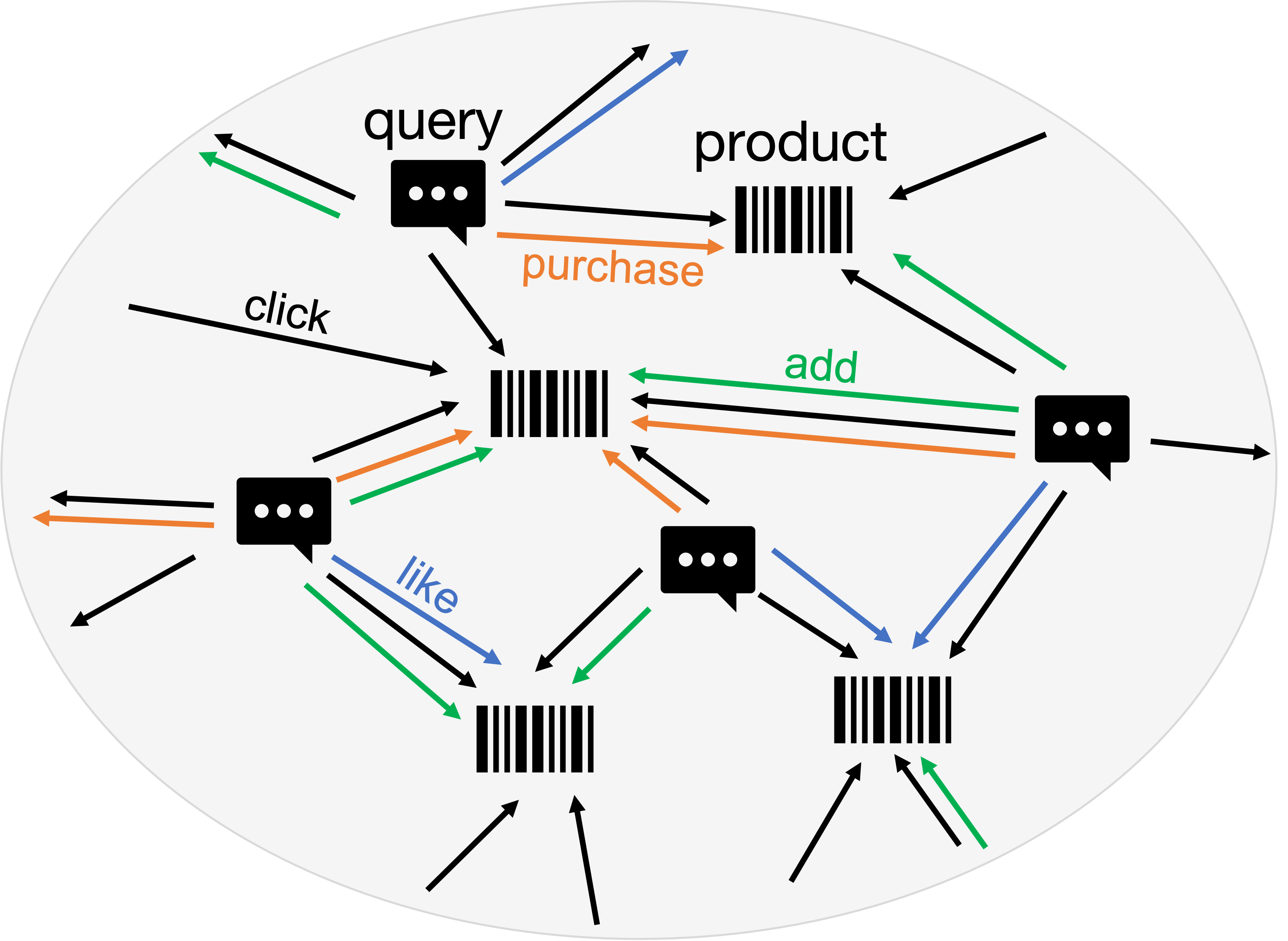
(a) A large graph corpus

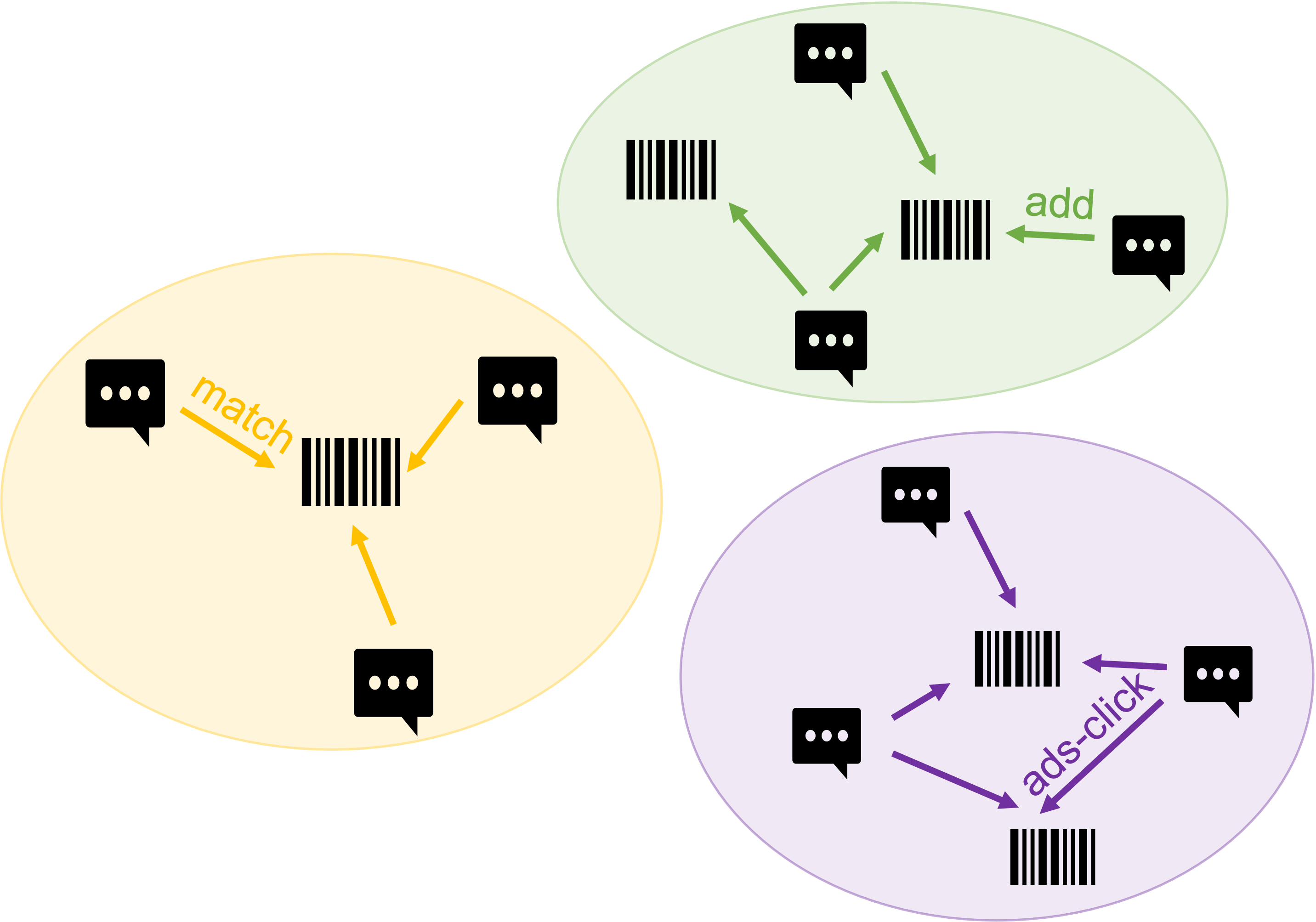
(b) Three application graphs

Figure 1. Toy examples of a large graph corpus and application graphs. The large graph covers most of the nodes in applications, while the edge types of applications can be distinct from the large graph.

We approach the key problem from two perspectives, pre-training a powerful model on a large graph corpus to capture the information that can maximize its utility towards a variety of applications, and fine-tuning the pre-trained model on various applications to further enhance its performance. Our main contributions include:

• We propose a framework of Graph-Aware LM pre-training on a large graph corpus, a.k.a. GaLM, which can encode knowledge in the large graph corpus into LMs under the consideration of entity relations in graphs.

• We propose various methods for fine-tuning the pre-trained GaLM on applications w.r.t. different modules of GaLM.

• We simulate a large graph corpus and two applications from a large public dataset; the comprehensive experiments on Amazon internal datasets and the public datasets demonstrate the effectiveness of our proposed pre-training/fine-tuning strategies.

• We provide insights into the empirical results, as well as additional analysis and discussion over the lessons learned.

In the rest of this paper, we discuss related works in Section 2. Section 3 introduces preliminaries including the problem formulation, the prevalent yet new concept of large graph corpus, and multiple related real applications that are deployed in Amazon. We then introduce the backbone model LM+GNN of our framework in Section 4. Sections 5 and 6 illustrate our proposed pre-training framework and fine-tuning strategies, respectively, and include empirical results and insights. Lastly, we provide an overall comparison and additional analysis in Section 7.

2. Related Works

2.1. Language Modeling with Graphs

Learning on graphs has attracted significant attention recently due to its capability of leveraging both node features and topological information to better model real-world applications. For language modeling, introducing the topological information that either models the real interactions (e.g., human behaviors) or semantic linkages (e.g., knowledge graphs, context) helps to overcome the inadequacy of utilizing solely pure semantic information. For example, (Shen et al., 2020; Wang et al., 2021; Yu et al., 2022; Ke et al., 2021; Yasunaga et al., 2022) leverage KGs as additional training signals to guide the learning of LMs, (Zhu et al., 2021a; Li et al., 2021) use behavior-graph augmented language modeling that is applied for sponsored search, and (Yao et al., 2019; Meng et al., 2022) construct graphs based on the raw text and represent the tokens or words as nodes.

Graph neural networks (GNNs) are widely-used techniques in graph representation learning, and some previous works of learning LMs with graphs employ GNNs to aggregate information that is propagated along the graph topology. However, how LMs and GNNs are combined can vary. For example, (Meng et al., 2022) encodes tokens using a vanilla neural LM and introduces the global context by constructing a heterogeneous graph with tokens as nodes and connecting tokens to their retrieved neighbors, which essentially stacks the GNNs on top of the vanilla LM without fine-tuning the LM. The LM performs the role of a static text encoder in this way of combining LMs and GNNs. (Zhu et al., 2021a; Li et al., 2021) both focus on sponsored search, of which (Li et al., 2021) first fine-tunes the pre-trained LMs by behavior-graph related tasks but still uses the fine-tuned LMs as static text encoders to generate fixed node features as the input into GNNs, while (Zhu et al., 2021a) leverages the behavior-graph as a complementary information and co-trains the parameters of LMs and GNNs. (Ioannidis et al., 2022) proposes a multi-step fine-tuning framework for LMs that can jointly train LMs and GNNs effectively and efficiently.

Different from the prior works, this work is generic and not application-specific, and not restricted to specific graph schema such as KGs. More importantly, it focuses on LM pre-training on a large graph corpus with graph information included and fine-tuning the pre-trained model on multiple applications where the edge schema can be distinct from the pre-training large graph.

2.2. Pre-training on Graphs

Many previous studies of pre-training on graphs concentrate on encoding the graph-level information into GNNs given enormous small graphs, especially in the molecule domain (e.g., (Hu* et al., 2020; Rong et al., 2020; Sun et al., 2022)). Apart from the graph-level pre-training, there emerge works studying pre-training on a large graph, which aim to address the problem of insufficient labels by self-supervised learning on the same graph (e.g., (Jiang et al., 2021b; Hwang et al., 2020; Hu et al., 2020b)), or to tailor the gap of optimization objectives and training data between self-supervised pre-training tasks and downstream tasks (e.g., (Han et al., 2021; Lu et al., 2021)), or to pre-train on a large graph to capture the transferable information for downstream application graphs (e.g., (Zhu et al., 2021b; Lu et al., 2021; Qiu et al., 2020; Fang et al., 2020; Jiang et al., 2021a)). Our setting is more proximate to the last category.

Among these works concerning transfer learning across graphs, (Zhu et al., 2021b) provides theoretical analysis for the transferability of GNNs and proposes a GNN transfer learning framework with ego-graph information maximization, (Lu et al., 2021) proposes a self-supervised pre-training strategy that learns fine-tuning during pre-training with a dual adaption mechanism at both node and graph levels, (Qiu et al., 2020) learns a universal and generic GNN model that can be applied to data from diverse domains and different tasks using contrastive learning (subgraph instance discrimination). However, all these works focus on homogeneous graphs. (Jiang et al., 2021a) first studies the pre-training of GNN on a large-scale heterogeneous graph with both node- and schema-level contrastive learning tasks that can be applied to in-domain new datasets. (Fang et al., 2020) proposes a generic pre-training framework for heterogeneous graphs by transforming the neighbors into sequences and adopting deep bi-directional transformers to encode them, under the supervision of masked node modeling and adjacent node prediction. However, these works concentrate on transferring across graphs with the same graph schema, while in our setting the application graphs can preserve new edge types distinct from the pre-training graph, which can enrich the set of applicable downstream tasks (e.g., predicting the new edge type) and introduce specific features to applications by involving new edge types. Moreover, most of the previous studies on pre-training with graphs omit the relationship between the raw text and graph topology and use node features that are generated in a graph-agnostic manner. In this work, we focus on leveraging graphs and GNNs to facilitate the information capturing of LMs on a large graph corpus.

3. Preliminaries

3.1. Problem Formulation

Given a large-scale heterogeneous graph with text information (the large graph corpus) $G_{\mathrm{c}}$, and multiple downstream application heterogeneous graphs $\mathcal{G}=\{g_{i}\}_{i=1}^{n}$, the goal is to leverage $G_{\mathrm{c}}$ to improve tasks on $g_{i}$.

We denote the large graph corpus as $G_{\mathrm{c}}=(V_{\mathrm{c}},E_{\mathrm{c}},A_{\mathrm{c}},R_{\mathrm{c}},\phi_{\mathrm{c}},\psi_{\mathrm{c}})$, and an application graph as $g_{i}=(V_{i},E_{i},A_{i},R_{i},\phi_{i},\psi_{i})$. $V_{\mathrm{c}}$ and $V_{i}$ are the node sets of $G_{\mathrm{c}}$ and $g_{i}$, respectively; $|V_{\mathrm{c}}|\gg|V_{i}|$ and $|V_{\mathrm{c}}\cap V_{i}|/|V_{i}|\lesssim 1$. The node sets $V_{\mathrm{c}}$ and $V_{i}$ are mapped by the node-type mapping functions $\phi_{\mathrm{c}}:V_{\mathrm{c}}\rightarrow A_{\mathrm{c}}$ and $\phi_{i}:V_{i}\rightarrow A_{i}$, respectively, where $A_{\mathrm{c}}$ and $A_{i}$ are the sets of node types, and $A_{i}\subseteq A_{\mathrm{c}}$. $E_{\mathrm{c}}$ and $E_{i}$ are the edge sets of $G_{\mathrm{c}}$ and $g_{i}$, which are mapped by the edge-type mapping functions $\psi_{\mathrm{c}}:E_{\mathrm{c}}\rightarrow R_{\mathrm{c}}$ and $\psi_{i}:E_{i}\rightarrow R_{i}$, respectively. $R_{\mathrm{c}}$ and $R_{i}$ are the sets of edge types of $G_{\mathrm{c}}$ and $g_{i}$, and they can be different from each other, i.e., $0\leq|R_{c}\cap R_{i}|\leq|R_{c}|$.

To leverage the large graph corpus $G_{\mathrm{c}}$, we pre-train a model that consists of an LM (or multiple LMs) and a multi-relational GNN on $G_{\mathrm{c}}$ using unsupervised learning, and aim to find the optimized model $\Theta_{\mathrm{c}}$ by minimizing the empirical loss

(1) $$\Theta_{\mathrm{c}}^{*}=\operatorname*{arg\,min}\mathcal{L}_{c}\left(F_{\mathrm{c}}(\Theta_{\mathrm{c}};G_{\mathrm{c}})\right).$$

In various scenarios, the number of LMs employed for modeling different types of nodes can vary. For example, previous knowledge shows that utilizing separate LMs to model different entities in e-commerce scenarios is effective (Zhu et al., 2021a; Li et al., 2021; Ioannidis et al., 2022). Herewith, we employ different LMs for query and product entities present in e-commerce data in this work.

The model $\Theta_{\mathrm{c}}$ is then fine-tuned on multiple tasks applied on $\mathcal{G}$ to improve their performance. For an application graph $g_{i}$, we initialize its model $\Theta_{i}$ by $\Theta_{\mathrm{c}}^{*}$, and then fine-tune $\Theta_{i}$ by minimizing its empirical loss

(2) $$\Theta_{\mathrm{i}}^{*}=\operatorname*{arg\,min}\mathcal{L}_{i}\left(F_{i}(\Theta_{i};g_{i})\right).$$

3.2. The Large Graph Corpus

The large graph corpus is a prevalent yet novel concept in this work. Generally, it is a heterogeneous graph in which nodes preserve text information and different types of edges can connect the same pairs of nodes. A toy example of a large graph corpus is shown in 1(a), that is, a user behavior graph from a shopping engine which includes the common user behaviors (e.g., “add”, “click”, “like”, and “purchase”) that happen between user-inputs “query” and items “product”. For example, the relation “add” between queries and products represents that users add items to their shopping carts under the queries, and the relation “like” represents that users show preferences for certain products and are more inclined to buy them. While the user behaviors are between the two node types of “query” and “product”, the large graph corpus can preserve more relation types that can be either between different node types or among the same node type. There are no specific constraints on the graph schema of a large graph corpus.

Regarding what downstream applications can benefit from the pre-training on a large graph corpus, it can be related to the node and relation types of the large graph corpus. From the perspective of node schema, the large graph corpus can support all applications whose task-required node types are a subset of its node types. However, it is more rigorous to consider the extent of relevance between the relation types of the large graph corpus and the relation types of downstream applications. In principle, it is not necessary for the relation types of applications to exactly be a subset of the relation types of the large graph corpus. As long as the information gathered through the relations in the large graph corpus is useful for the applications, it should be beneficial to pre-train a model on the large graph corpus. The nodes in the large graph corpus are associated with abundant text information that can be highly complicated, thus, we utilize large LMs to encode the text information. Herewith, we expect that the pre-trained LMs with rich relational information on the large graph corpus can generalize to accommodate a variety of downstream applications with different tasks.

3.3. Multiple Applications

We employ various applications with different tasks to investigate how the pre-training on a large graph corpus aids in downstream applications. 1(b) shows example graphs of several applications. It is usual that applications preserve a small number of relation types (e.g., one or two), and the relation types can be distinct from those of the large graph corpus. For empirical studies, we form a dataset group Amazon-PQ using Amazon internal datasets, which consists of a large graph corpus for pre-training, and three real applications, Search-CTR, ESCvsI, and Query2PT.

Search-CTR. It is an application to predict whether a user/query would click an advertised product or not, which can be modeled as a link prediction task. Its application graph contains node types “product” and “query”, and an edge type “ads-click” which is defined as the click-through rate and differs from the common “click”.

ESCvsI. It is an application for the query-product matching problem. Its graph contains node types “query” and “product” and an edge type “match”. Edges are originally labeled as E (exact), S (substitute), C (complement), and I (irrelevant); however, the task in this work is to classify the edges connecting query-product pairs into one of the two classes, E/S/C and I, i.e., edge classification.

Query2PT. It is an application to predict the types of products that are mapped to a query. Its graph contains the edge type “click” and node types “query” and “product”, and the task of the application is to classify the “query” nodes by multiple labels (out of 403 classes), i.e., multi-label node classification.

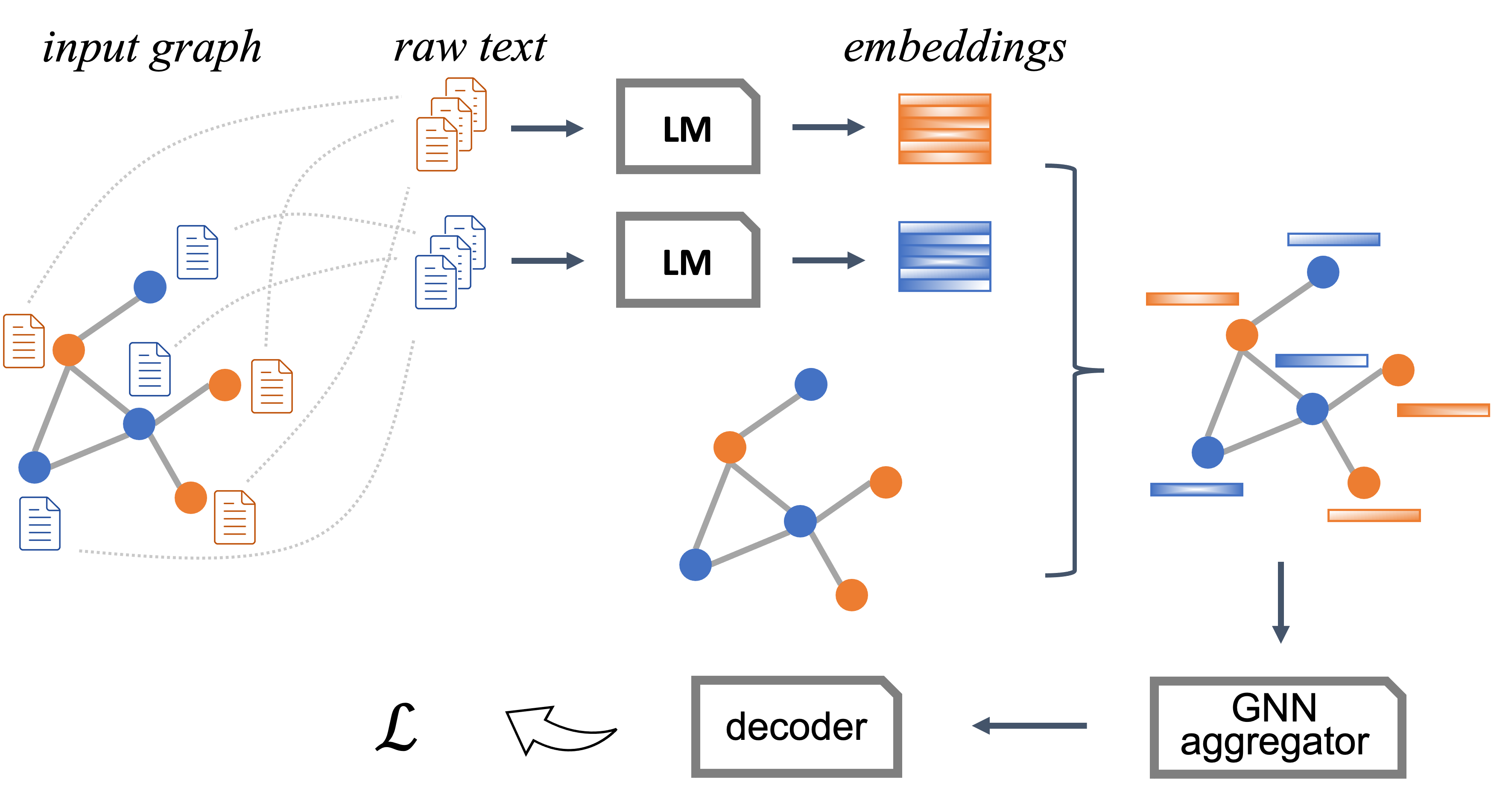
Figure 2. The backbone model LM+GNN. Nodes in different colors belong to different node types. The raw text is encoded using an LM or multiple LMs w.r.t. different node types. The output of LMs is then encoded by a GNN aggregator based on the graph topology and finally decoded for a graph-based task.

The data statistics of Amazon-PQ are shown in Table 6 in Appendix A.1. The large graph corpus and application graphs are strategically down-sampled from the original Amazon internal datasets, which are then aggregated and anonymized, and are not representative of real product traffic. The sampling details are discussed in Section 7.1.2.

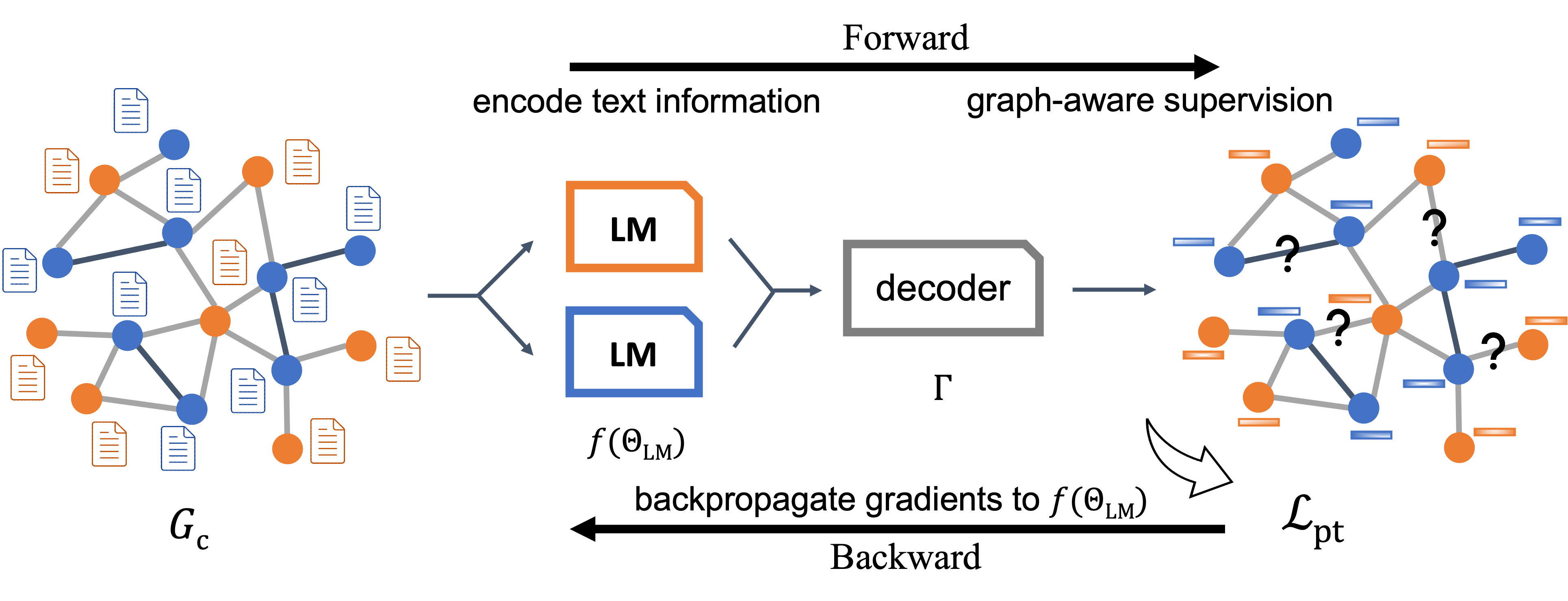
(a) A GNN-free GaLM

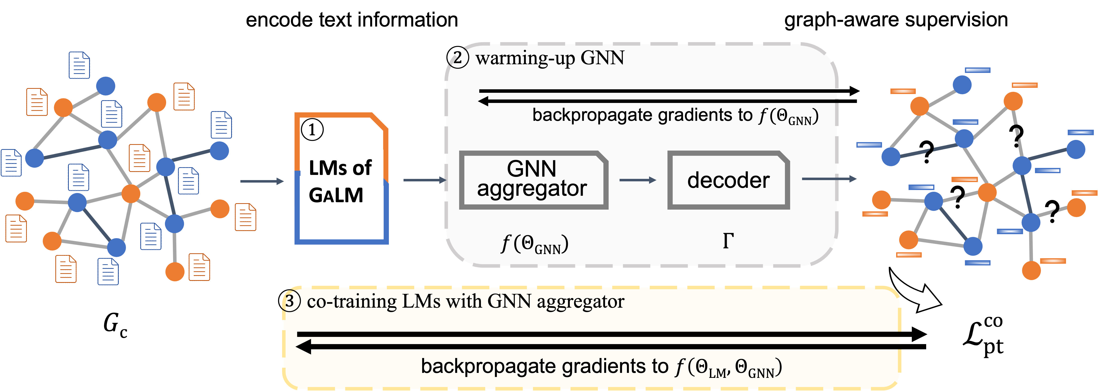
(b) A GNN-co-trained GaLM: $\mathrm{\textsc{GaLM}^{co}}$

Figure 3. Graph-aware LM pre-training framework (GaLM). The LMs are pre-trained on a given large graph corpus either with or without the incorporation of GNN aggregators ($\mathrm{\textsc{GaLM}^{co}}$ or GaLM, respectively). (a) The pre-training of GaLM further trains existing general LMs in a graph-aware manner. (b) The pre-training of $\mathrm{\textsc{GaLM}^{co}}$ includes three steps: i. fine-tuning existing general LMs by graph-aware supervision, ii. warming up the GNN aggregator by fixing the graph-aware pre-trained LMs, iii. co-training the graph-aware pre-trained LMs with the warmed-up GNN aggregator by end-to-end backpropagating the loss to LMs through GNN.

4. LM+GNN: The Backbone of Our Proposed Framework

The backbone model of our framework for learning on graph corpora is defined as LM+GNN, which consists of one or more LMs for encoding text information and a GNN aggregator for information aggregation. Figure 2 shows the pipeline of LM+GNN. Given a graph corpus as the input, LM+GNN employs one or multiple LMs as text encoder(s) for nodes. Through the LMs, the generated embeddings are then attached to the graph topology as the input of a GNN aggregator, and the output is passed through a task-specific decoder for supervision.

The LMs here can be adapted to various pre-trained large language models. We implement the LMs with BERT in this work because it is well-studied in most existing related works and widely applied in the industry.

The GNN aggregator can also be adapted to different GNN variants, such as GCN and GAT for graphs with only one type of relation, and RGCN and RGAT for graphs with multiple types of relations. The GNN aggregator in the pipeline aids in the propagation of information based on the graph topology. Regarding multi-relational graphs, which are more generic and adopted in this work, we implement the GNN aggregators with two common relational GNNs, RGCN (Schlichtkrull et al., 2018) and RGAT (Busbridge et al., 2019). The propagation rule of RGCN is

(3) $$h_{u}^{(l+1)}=\sigma\left(\sum_{r\in R}\sum_{v\in\mathcal{N}_{u}^{r}}\frac{1}{c_{u,r}}\Theta_{r}^{(l)}h_{v}^{(l)}+\Theta_{0}^{(l)}h_{u}^{(l)}\right),$$

where $h_{u}^{(l)}$ is the representation of node $u$ at the layer $l$, and node $v$ is a neighbor of node $u$ that is connected by an edge with relation $r$. The normalization constant can be customized w.r.t. specific tasks, such as $c_{u,r}=|\mathcal{N}_{u}^{r}|$ for entity classification task, and $c_{u,r}=\sum_{r}|\mathcal{N}_{u}^{r}|$ for link prediction task. For RGAT, it introduces the attention mechanism into RGCN and learns the normalized attention coefficients for aggregating neighborhood information with attention.

In the vanilla LM+GNN model, the LMs and a GNN aggregator are simply stacked, and the two processes of encoding text information and aggregating neighborhood information are separate.

5. Graph-aware LM Pre-training on a Large Graph Corpus

The pre-training on a large graph corpus aims to capture as much information as possible that can aid in a variety of downstream applications. As LMs retain a significant number of parameters that can understand the text information well, and graph topology conserves the correlation between entities that can be meaningful for propagating information, we propose a Graph-Aware LM pre-training framework (a.k.a. GaLM) to combine their advantages. Pre-training GaLM on a large graph corpus can incorporate the graph information into the fine-tuning of existing pre-trained LMs that are pre-trained on general texts (such as the BERT model). Although it is in fact fine-tuning existing pre-trained LMs on a large graph corpus, we define it as graph-aware LM pre-training from the perspective of our overall framework. The pipeline of GaLM is displayed in Figure 3.

5.1. Graph-aware LM Pre-training

Graph-aware LM pre-training (GaLM) aims to pre-train LMs on a large graph corpus with its graph information being absorbed in the LMs. A straightforward way of incorporating the graph information into LM pre-training is utilizing graph tasks for supervision. 3(a) displays the pipeline of a GaLM. Given a large graph corpus, its attached raw text information is encoded by the general pre-trained LMs. As separate LMs are usually employed for query and product entities in e-commerce scenarios, we introduce our framework by the way that separate LMs are responsible for different node types of the large graph corpus in the following. The output embeddings of LMs are then associated with the graph topology as the inputs of a graph-task-specific decoder. The full forward pass is supervised by the graph task and computes the loss

(4) $$\mathcal{L}_{\mathrm{pt}}=\ell\left(\Gamma\left(\Theta_{\mathrm{de}};f(\Theta_{\mathrm{LM}};G_{\mathrm{c}})\right)\right),$$

where $\Theta_{\mathrm{LM}}$ and $\Theta_{\mathrm{de}}$ are the parameters of the LMs and the decoder $\Gamma$ of GaLM, and $\ell$ is the task-specific loss. In this work, we employ the typical unsupervised learning task for pre-training on a large graph corpus, i.e., link prediction. Specifically, the loss for a link prediction task is computed by

(5) $$\hat{y}_{e_{uv}}=\Gamma(\Theta_{\mathrm{de}};h_{u}\oplus h_{v}),$$

(6) $$\mathcal{L}_{\mathrm{pt}}=-\sum_{e_{uv}\in E_{\mathrm{c}}^{\mathrm{train}}}\left(y_{e_{uv}}\log(\hat{y}_{e_{uv}})+(1-y_{e_{uv}})\log(1-\hat{y}_{e_{uv}})\right),$$

where $h_{u}$ and $h_{v}$ are the output embeddings of the LMs of GaLM. In the backward process, the loss $\mathcal{L}_{\mathrm{pt}}$ of the forward propagation will be backpropagated to the LMs by using the gradients to fine-tune the parameters of LMs.

To investigate whether the graph-aware pre-training on the large corpus is effective in promoting multiple applications, we compare the pre-trained GaLM with two baseline models, $\mathrm{\textsc{LM}_{\textsc{(Bert-base)}}}$ and $\mathrm{\textsc{LM}_{\textsc{(Bert-mlm)}}}$, by applying them to several applications with different tasks. The model $\mathrm{\textsc{LM}_{\textsc{(Bert-base)}}}$ is initialized from the public BERT model that is pre-trained on English language in the general domain using masked language modeling (MLM) objective, and the model $\mathrm{\textsc{LM}_{\textsc{(Bert-mlm)}}}$ is further trained based on $\mathrm{\textsc{LM}_{\textsc{(Bert-base)}}}$ using the text information alone from our large graph corpus (aggregated node features without graph structures) by MLM. From Table 1, it is obvious that GaLM significantly improves the applications by comparing to $\mathrm{\textsc{LM}_{\textsc{(Bert-base)}}}$ and $\mathrm{\textsc{LM}_{\textsc{(Bert-mlm)}}}$, which indicates that the graph-aware LM pre-training on a large graph corpus is capable of capturing useful information that could be beneficial to downstream applications. Additionally, the finding demonstrates the key point of GaLM that distinguishes our work from the priors, which focuses on how the pre-training, especially, the graph-aware LM pre-training acts in helping with multiple applications.

Table 1. The effect of graph-aware LM pre-training. Due to company regulations, the results of $\mathrm{\textsc{LM}_{\textsc{(Bert-base)}}}$ baseline are set to zeros, and other baselines and GaLM models report relative increases from it.

Models	Search-CTR	ESCvsI	Query2PT
	(ROC-AUC)	(macro-F1)	(macro-F1)
$\mathrm{\textsc{LM}_{\textsc{(Bert-base)}}}$	0.00	0.00	0.00
$\mathrm{\textsc{LM}_{\textsc{(Bert-mlm)}}}$	0.31%	-0.24%	19.00%
GaLM	2.54%	2.78%	32.88%
$\mathrm{\textsc{GaLM}^{co_{(rgcn)}}}$	3.00%	3.55%	30.38%
$\mathrm{\textsc{GaLM}^{co_{(rgat)}}}$	3.16%	2.95%	32.80%

• * The rule is applied to all results evaluated on internal applications of Amazon-PQ due to the legal issue.

5.2. GNN-based Graph-aware LM Pre-training

Another natural alternative to incorporating graph information into LMs is co-training LMs with a GNN aggregator. In addition to the aforementioned way of using graph tasks as the supervision, co-training LMs with a GNN aggregator performs the end-to-end training on pre-trained LMs. However, it is known that the end-to-end training of LMs with GNNs can be extremely time-consuming, especially on a large graph corpus. Thus, we choose to only backpropagate on samples in the co-training process. To accelerate the overall converging speed, we perform two additional steps before co-training by infusing LMs with graph information overhead. We first fine-tune existing general LMs on the large graph corpus by graph-aware supervision. Then, we warm up the GNN aggregator to prevent the co-training from settling on undesirable local minima as the LMs are optimized (also discussed in (Ioannidis et al., 2022)).

3(b) details the pipeline of the GNN-based graph-aware LM pre-training (we term it as $\mathrm{\textsc{GaLM}^{co}}$), which includes the training of a vanilla GaLM (see Section 5.1), warming up a GNN aggregator, and co-training the pre-trained LMs of GaLM with the warmed-up GNN aggregator. The GNN warming-up step follows LM+GNN (see Section 4), which fixes the LMs of a vanilla GaLM and trains a GNN aggregator with link prediction. Empirical studies show that a fixed number of epochs (e.g., 2 or 3) is sufficient for warming up. In the co-training step, the forward pass computes the loss

(7) $$\mathcal{L}_{\mathrm{pt}}^{\mathrm{co}}=\ell(\Gamma(\Theta_{\mathrm{de}};f(\Theta_{\mathrm{LM}},\Theta_{\mathrm{GNN}};G_{\mathrm{c}}))),$$

and the backward pass will backpropagate the gradients on some samples from the GNN aggregator to the LMs.

To study whether the GNN-based graph-aware LM pre-training will further promote the applications, we adopt two types of GNN aggregators into $\mathrm{\textsc{GaLM}^{co}}$, RGCN (Schlichtkrull et al., 2018) and RGAT (Busbridge et al., 2019), and compare the performance of the LMs from $\mathrm{\textsc{GaLM}^{co}}$ ($\mathrm{\textsc{GaLM}^{co_{(rgcn)}}}$ and $\mathrm{\textsc{GaLM}^{co_{(rgat)}}}$) to those from the vanilla GaLM on applications, as shown in Table 1. In general, $\mathrm{\textsc{GaLM}^{co}}$ performs similarly to the vanilla GaLM on the applications. We observe a slight improvement of $\mathrm{\textsc{GaLM}^{co}}$ on Search-CTR, but it does not show superiority on ESCvsI and Query2PT. Since $\mathrm{\textsc{GaLM}^{co}}$ is comparable to a vanilla GaLM on downstream applications but is more time-consuming (see Appendix B.1), we deem it more reasonable to choose the vanilla graph-aware LM pre-training method rather than the GNN-based one for pre-training on a large graph corpus, considering the restrictions of computation and time resources.

6. GaLM Fine-tuning on Multiple Graph Applications

We demonstrated the effectiveness of GaLM in Section 5 by directly applying its graph-aware-pre-trained LMs to various applications. In this section, furthermore, we investigate how the GaLM can be fine-tuned to further improve the performance on multiple graph applications. As the architecture of a GaLM consists of (node-type-specific) LMs, an optional relation-type-specific GNN aggregator, and a task-specific decoder, the fine-tuning of a GaLM can involve fine-tuning LMs of GaLM, along with training or fine-tuning a GNN aggregator. The proposed fine-tuning methods of GaLM are illustrated in Figure 4.

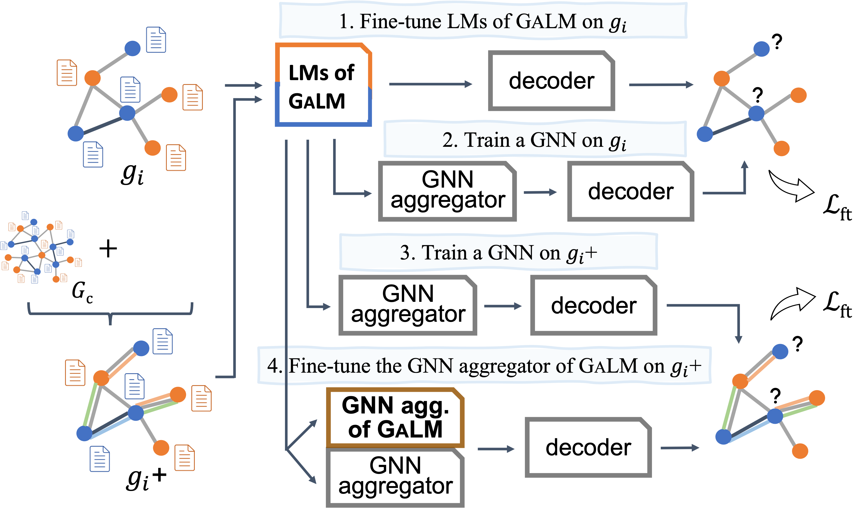
Figure 4. Fine-tuning strategies. Step 1: Graph-aware LM fine-tuning on applications using the pre-trained GaLM; Step 2: Fine-tuning GaLM (or $\mathrm{\textsc{GaLM}^{*}}$) on an application by training a GNN aggregator; Step 3: Stitching an application graph with the large graph and training a GNN aggregator on the stitched application graph; Step 4: Fine-tuning the GNN aggregator of GaLM on a stitched application graph.

6.1. Fine-tuning GaLM on Applications

To fine-tune the pre-trained GaLM on applications, the proposed methods can be 1) further fine-tuning the LMs of GaLM on graph applications, and 2) training a new GNN aggregator on application graphs employing the LMs of GaLM.

6.1.1. Graph-aware LM fine-tuning on applications

Similar to Section 5.1, we adopt the graph information into the LM fine-tuning on applications (Step 1 in Figure 4). Given an application graph with raw text, we use the LMs from a pre-trained GaLM to encode the raw text, whose output embeddings are then input into an application-specific decoder. The forward pass is supervised by a particular graph task that varies depending on applications. For example, for an application graph $g_{i}$ with a node classification task, the loss of its graph-aware LM fine-tuning is computed by

(8) $$\mathcal{L}_{\mathrm{ft}}=\sum_{u\in V_{i}^{\mathrm{train}}}-\log\left(\operatorname*{softmax}(y_{u},\hat{y}_{u})\right);$$

for an application with an edge classification task, its loss can be computed using the Equation 5 and 6.

To study how the graph-aware fine-tuning of LMs from GaLM helps various applications, we fine-tune the pre-trained GaLM on applications of Amazon-PQ with diverse graph tasks. The fine-tuned model is denoted as $\mathrm{\textsc{GaLM}^{*}}$. As can be observed from Table 2, $\mathrm{\textsc{GaLM}^{*}}$ slightly improves GaLM on Search-CTR and ESCvsI, but significantly outperforms GaLM on Query2PT. The reason can be that Search-CTR and ESCvsI conduct similar link-level tasks to GaLM during its pre-training on a large graph corpus, while Query2PT conducts a multi-label node classification task that differs more from GaLM’s pre-training task. Hence, Search-CTR and ESCvsI can barely gain extra information from fine-tuning LMs of GaLM on the application graph, while Query2PT can still obtain beneficial new information.

Additionally, although we have shown the direct benefit of pre-training LMs on a large graph corpus without fine-tuning on the application graph (Table 1), it might be interesting to see what if the generic LMs are directly fine-tuned on the application graph. To this end, we perform graph-aware LM fine-tuning using the public BERT model on these applications, as denoted by $\mathrm{\textsc{LM}_{\textsc{(Bert-base)}}^{*}}$ in Table 2. By comparing $\mathrm{\textsc{GaLM}^{*}}$ and $\mathrm{\textsc{LM}_{\textsc{(Bert-base)}}^{*}}$, it is evident that the pre-training on the large graph corpus can benefit the applications to varying extents depending on the applications.

Table 2. The effect of fine-tuning GaLM on applications.

Models	Search-CTR	ESCvsI	Query2PT
	(ROC-AUC)	(macro-F1)	(macro-F1)
$\mathrm{\textsc{LM}_{\textsc{(Bert-base)}}^{*}}$	1.58%	2.92%	4.89%
GaLM	2.54%	2.78%	32.88%
$\mathrm{\textsc{GaLM}^{*}}$	3.04%	3.89%	41.20%
$\mathrm{\textsc{GaLM}^{*}_{rgcn}}$	4.46%	4.96%	61.06%
$\mathrm{\textsc{GaLM}^{*}_{rgat}}$	17.49%	10.89%	66.50%

6.1.2. Fine-tuning GaLM with GNNs on applications

As the graph-aware LM fine-tuning on applications can encode the graph information into LMs to some extent, it is interesting to explore whether leveraging an extra GNN aggregator to propagate information is still desirable. We regard this method of training application-specific GNN aggregators using LMs of $\mathrm{\textsc{GaLM}^{*}}$ as fine-tuning GaLM with GNNs on applications. In principle, the fine-tuning can be realized by training a standalone GNN aggregator using the LMs of $\mathrm{\textsc{GaLM}^{*}}$ or co-training a GNN aggregator with the LMs. Considering the trade-offs between utility and efficiency, it is reasonable to choose the former (Step 2 in Figure 4), where we use the LMs of $\mathrm{\textsc{GaLM}^{*}}$ to generate embeddings for nodes of an application graph, and train a GNN aggregator and a task-specific decoder on the application graph with the generated embeddings as input features.

To investigate the effect of fine-tuning GaLM with GNNs on applications, we further fine-tune a $\mathrm{\textsc{GaLM}^{*}}$ with RGCN and RGAT on the internal applications, as denoted by $\mathrm{\textsc{GaLM}^{*}_{rgcn}}$ and $\mathrm{\textsc{GaLM}^{*}_{rgat}}$, respectively. From Table 2, the improvements brought by $\mathrm{\textsc{GaLM}^{*}_{rgcn}}$ and $\mathrm{\textsc{GaLM}^{*}_{rgat}}$ are significant compared to $\mathrm{\textsc{GaLM}^{*}}$, which indicates that fine-tuning $\mathrm{\textsc{GaLM}^{*}}$ by training GNN aggregators on applications is profitable.

6.2. Fine-tuning GaLM on Applications Stitched with the Large Graph Corpus

Apart from fine-tuning GaLM with GNNs on applications at the model level, another way to inject graph information is by stitching application graphs with the large graph corpus at the data level (we term the resulting graphs as stitched application graphs, $\{g_{i}+\}$). Since the large graph corpus preserves more edge types and many more edges that are not included in applications, stitching application graphs with the large graph would introduce more neighbors for nodes in applications, which could benefit their gathering of neighborhood information.

To stitch an application graph with the large graph corpus, we align the overlapped nodes between the application graph and the large graph via internal entity IDs, and then add the connecting edges of these overlapped nodes that appear in the large graph into the application graph.

6.2.1. Fine-tuning GaLM with GNNs on stitched application graphs

Similar to Section 6.1.2, fine-tuning GaLM with GNNs on a stitched application graph aims to train a GNN aggregator with an application-specific decoder on the stitched application graph utilizing pre-trained LMs of GaLM (Step 3 in Figure 4). Here, we employ LMs of $\mathrm{\textsc{GaLM}^{*}}$ to generate node embeddings and train a GNN aggregator and decoder on the stitched application graph; the fine-tuned models are $\mathrm{\textsc{GaLM}^{*}_{rgcn}}$+ and $\mathrm{\textsc{GaLM}^{*}_{rgat}}$+, respectively.

From Table 3, both $\mathrm{\textsc{GaLM}^{*}_{rgcn}}$+ and $\mathrm{\textsc{GaLM}^{*}_{rgat}}$+ are apparently superior to $\mathrm{\textsc{GaLM}^{*}_{rgcn}}$ and $\mathrm{\textsc{GaLM}^{*}_{rgat}}$, respectively, which indicates that applications can benefit from introducing more neighborhood information from the large graph corpus. On the other hand, the superiority of $\mathrm{\textsc{GaLM}^{*}_{rgnn}}$+ over $\mathrm{\textsc{GaLM}^{*}_{rgnn}}$ implies that the model-level graph-aware LM pre-training on the large graph corpus using link prediction is insufficient for capturing all the graph information from the large graph corpus. Consequently, enhancing the training of GNN aggregators at data level on the stitched application graphs with extra edges from the large graph using $\mathrm{\textsc{GaLM}^{*}}$ can further improve the performance of applications. However, it remains an open question whether the graph information of the large graph corpus can be fully captured through more dedicated designs of LMs and graph-aware pre-training, which could be explored in future work.

Table 3. The effect of fine-tuning $\mathrm{\textsc{GaLM}^{*}}$ with GNNs on stitched application graphs.

Models	Search-CTR	ESCvsI	Query2PT
	(ROC-AUC)	(macro-F1)	(macro-F1)
$\mathrm{\textsc{GaLM}^{*}_{rgcn}}$	4.46%	4.96%	61.06%
$\mathrm{\textsc{GaLM}^{*}_{rgat}}$	17.49%	10.89%	66.50%
$\mathrm{\textsc{GaLM}^{*}_{rgcn}}$+	13.38%	8.19%	76.39%
$\mathrm{\textsc{GaLM}^{*}_{rgat}}$+	20.37%	13.35%	80.06%

6.2.2. Fine-tuning GaLM with pre-trained GNNs on stitched application graphs

As discussed in Section 5.2, in the stage of pre-training on a large graph corpus, besides LMs, GaLM can also pre-train a standalone GNN aggregator or co-training a GNN aggregator with the LMs. Thus, it is natural to investigate whether the pre-trained GNN aggregator can be fine-tuned on applications, especially under the consideration of training efficiency. However, due to the inconsistency of edge types between the applications and the large graph, the pre-trained GNN aggregator that models the specific types of edges in the large graph cannot be directly fine-tuned on the application graphs. A proposed method is to first include the original edge distribution in applications, that is, to stitch application graphs with the large graph; then, in addition to inheriting the pre-trained GNN aggregator for the original types of edges in the large graph, we initialize a new GNN aggregator for the new types of edges in the application graphs (Step 4 in Figure 4).

The proposed method of fine-tuning the pre-trained GNN aggregator on stitched application graphs seems to be straightforward. However, it in fact involves complex decision-making– for example, how to choose a combination of the learning rates for fine-tuning the pre-trained GNN aggregator and training the newly initialized GNN aggregator, which would affect how much information from the pre-training to be retained; how to initialize the new GNN aggregator, where different initializations may impact the optimizing; and how to aggregate the outputs of the pre-trained and the newly initialized GNN aggregators, which can be a simple operation (e.g., summation, average, and concatenation) or parameterized and to be learned. We deem these complicated decisions beyond the scope of this work and will only provide preliminary results and leave the further explorations in future work.

Albeit the complex decision-making, we attempted some simple decisions to fine-tune the pre-trained GNN aggregator using $\mathrm{\textsc{GaLM}^{*}}$, i.e., initializing the new GNN aggregator at Xavier’s random (Glorot and Bengio, 2010), summing up the outputs of the pre-trained and new initialized GNN aggregators for the same nodes, and tuning the learning rate of the GNN fine-tuning to tens, hundreds, or thousands of times smaller than the learning rate of the new GNN aggregator. The fine-tuned model $\mathrm{\textsc{GaLM}^{**}_{rgat}}$+ in Table 4 displays the best results according to our limited attempts based on the aforementioned simple decisions. In general, the $\mathrm{\textsc{GaLM}^{**}_{rgat}}$+ model is found comparable but slightly inferior to $\mathrm{\textsc{GaLM}^{*}_{rgat}}$+ on the stitched application graphs. On the other hand, we observe that fine-tuning the pre-trained GNN aggregator of GaLM on stitched application graphs may indeed lead to faster convergence. For example, $\mathrm{\textsc{GaLM}^{**}_{rgat}}$+ converges to 97% of the best performance on Search-CTR after $600$ iterations while $\mathrm{\textsc{GaLM}^{*}_{rgat}}$+ needs $13,800$ iterations to converge to the same level, where the elapsed time of every iteration is roughly the same across the two frameworks.

Table 4. The effect of fine-tuning $\mathrm{\textsc{GaLM}^{*}}$ with pre-trained GNNs on stitched application graphs.

Models	Search-CTR	ESCvsI	Query2PT
	(ROC-AUC)	(macro-F1)	(macro-F1)
$\mathrm{\textsc{GaLM}^{*}_{rgat}}$+	20.37%	12.99%	80.06%
$\mathrm{\textsc{GaLM}^{**}_{rgat}}$+	19.93%	11.34%	77.25%

7. External and Overall Evaluations

7.1. Public Data Source

To solidify our pre-training and fine-tuning methods, apart from the Amazon internal dataset Amazon-PQ, we simulate a large graph corpus and corresponding application graphs using a public dataset, Amazon Product Reviews with the time span from May 1996 to July 2014, which we name them together as Product-Reviews dataset. The original Amazon Product Reviews dataset is large, so we select some fields of text and down-sample records of items and reviews.

7.1.1. Data partitioning

Upon the enormous raw text, we concatenate the selected fields “title”, “brand”, “feature”, and “description”, as the raw text of items, and select the field “reviewText” as the raw text of reviews. We also retain the field “categories” as the targets of items for an application task of predicting the product type of items.

The filtered text is then partitioned into a large graph corpus and multiple applications, based on their node and edge schemas. For Product-Reviews, the node schema is defined as {“asin”, “reviewText”}. In the large graph corpus, the edge schema is {“asin–coview–asin”, “reviewText–review–asin”, “reviewText–cowrite–reviewText”}, which separately represent that a reviewText reviews an item, two reviewTexts are written by the same reviewer, and an item is also viewed when its connected item is reviewed. We simulate two application graphs according to the real-world applications, CoPurchase and Product2PT. The new edge type in CoPurchase and Product2PT is “asin–cobuy–asin”, which represents that a user bought both the connected two items. Herewith, the application of CoPurchase is to predict whether users would buy two items together, which performs as a link prediction task; and the Product2PT application is to predict the product type of items, which performs as a node classification task.

7.1.2. Graph down-sampling

Instead of sampling records directly from the filtered text, which could lead to largely disturbed graph structures and extremely sparse edges, we first construct the large graph and application graphs using all filtered text and then down-sample the constructed graphs. The sampling begins with a random set of nodes and samples their neighbors; the sampled neighbors are then used as the starting set of nodes for sampling neighbors one hop further. After iterating the process several times, we extract all edges from the initially constructed graph whose two-end nodes are within the set of sampled nodes; hereby, the edges that are connected by the sampled nodes but are not sampled during the iteration of sampling will be also included in the sampled graph, to avoid generating a collection of disconnected k-hop networks. The data statistics of the sampled large graph corpus and application graphs are shown in Table 7 in Appendix A.2.

7.2. Implementation Details

As the original Amazon internal datasets and the public Amazon Product Reviews dataset are both very large, their preprocessing including down-sampling is implemented on distributed Spark framework. The experiments use a cluster of 64 Nvidia Tesla V100 32GB GPUs. The hyper-parameter settings for models and experiments are shown in Table 8 in Appendix B.2.

7.3. Results on Internal and Public Datasets

Table 5. The overall comparison of models using $\mathrm{\textsc{GaLM}_{rgat}}$ on Amazon-PQ and Product-Reviews. The LMs in models without a “*” are not fine-tuned on applications.

Models	Amazon-PQ			Product-Reviews
	Search-CTR	ESCvsI	Query2PT	CoPurchase	Product2PT
	(ROC-AUC)	(macro-F1)	(macro-F1)	(MRR)	(macro-F1)
$\mathrm{\textsc{LM}_{\textsc{(Bert-base)}}}$ +$\mathrm{\textsc{Gnn}_{(rgat)}}$	15.60%	8.51%	39.56%	0.1941	0.7038
$\mathrm{\textsc{LM}_{\textsc{(Bert-base)}}^{*}}$ +$\mathrm{\textsc{Gnn}_{(rgat)}}$	15.47%	6.49%	44.84%	0.3230	0.7479
$\mathrm{\textsc{GaLM}_{rgat}}$	17.30%	10.39%	64.03%	0.3461	0.7317
$\mathrm{\textsc{GaLM}^{*}_{rgat}}$	17.49%	10.89%	66.50%	0.3474	0.7491
$\mathrm{\textsc{GaLM}^{*}_{rgat}}$+	20.37%	13.35%	80.06%	0.4542	0.7813

From the previous observations, fine-tuning GaLM with GNNs can dramatically improve the performance of applications. Thus, we select the better model of $\mathrm{\textsc{GaLM}_{rgat}}$ and implement different fine-tuning methods upon it, to obtain an overall comparison on both internal Amazon-PQ and public Product-Reviews datasets (see Table 5). The baselines are implemented as the backbone LM+GNN using public pre-trained LMs, and all the GNN aggregators incorporate RGAT. The models $\mathrm{\textsc{GaLM}^{*}_{rgat}}$ and $\mathrm{\textsc{GaLM}^{*}_{rgat}}$+ are as described in Section 6, which fine-tune the pre-trained LMs of GaLM on applications in a graph-aware manner and then train GNN aggregators on application graphs and stitched application graphs, respectively, while $\mathrm{\textsc{GaLM}_{rgat}}$ uses the pre-trained LMs of GaLM without further fine-tuning on application graphs.

From the results, it further confirms that the graph-aware LM pre-training on a large graph corpus and fine-tuning on applications can be beneficial to these applications with various tasks, as can be observed where most GaLM variants perform significantly better on all five applications in comparison to the $\mathrm{\textsc{LM}_{\textsc{(Bert-base)}}}$ variants. Besides, the superiority of $\mathrm{\textsc{GaLM}^{*}_{rgat}}$+ over $\mathrm{\textsc{GaLM}^{*}_{rgat}}$ demonstrates the effectiveness of introducing more neighborhood information of the large graph corpus to applications at the data level, which can assist the information propagation of GNN aggregators on applications with the extra information that is not fully captured by the model-level graph-aware pre-training. It is also noticeable that when fine-tuning GaLM with GNN aggregators on applications, it could be unnecessary to directly fine-tune the LMs of GaLM on application graphs, as can be observed where $\mathrm{\textsc{GaLM}^{*}_{rgat}}$ performs similarly to $\mathrm{\textsc{GaLM}_{rgat}}$. The reason could be that the capacity of GNN aggregators is sufficient for capturing essential information of the application graphs, thus, training GNN aggregators using $\mathrm{\textsc{GaLM}^{*}}$ does not provide much additional gain over GaLM.

7.4. Additional Analysis

7.4.1. Significance test

Regarding the overall comparison in Table 5, we conduct a significance analysis to confirm the significance of the superiority of our proposed frameworks compared to the baselines. We run five repetitions on the public application Product2PT for each model (the original results are in Table 9 in Appendix B.3), and then perform a one-sided T-test (Student, 1908) between each pair of models. By one-sided T-test, we test whether one model performs significantly better than another model rather than only testing whether they are significantly different. 5(a) displays the heatmap of p-values from the pair-wise one-sided T-tests. According to the heatmap, most of the comparison is significant as the p-value is less than 0.05. A noticeable result is the p-value of 1.0 between $\mathrm{\textsc{LM}_{\textsc{(Bert-base)}}^{*}}$ +$\mathrm{\textsc{Gnn}_{(rgat)}}$ and $\mathrm{\textsc{GaLM}_{rgat}}$, which indicates that the alternative hypothesis that $\mathrm{\textsc{GaLM}_{rgat}}$ is significantly better than $\mathrm{\textsc{LM}_{\textsc{(Bert-base)}}^{*}}$ +$\mathrm{\textsc{Gnn}_{(rgat)}}$ is rejected. It can be because the Product2PT dataset is relatively small and simple (with a single type of nodes and edges), and the fine-tuning of public pre-trained LMs on it combing with training a GNN aggregator is capable to capture adequate information for its task, so $\mathrm{\textsc{LM}_{\textsc{(Bert-base)}}^{*}}$ +$\mathrm{\textsc{Gnn}_{(rgat)}}$ can achieve a comparable result to the $\mathrm{\textsc{GaLM}^{*}_{rgat}}$ model.

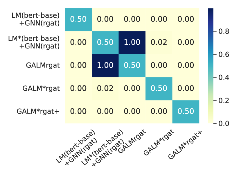
(a) The p-values on Product2PT.

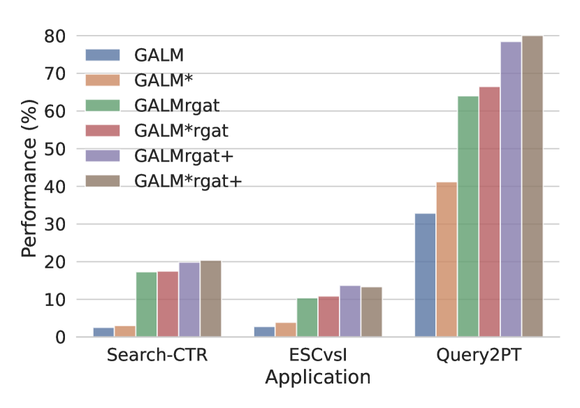
(b) Model performance on Amazon-PQ applications.

Figure 5. Additional analysis. (a) Significant test. The p-values are calculated using one-sided pair-wise T-tests (the alternative hypothesis is that the model performs worse than the model below it or on the right side of it). (b) Ablation studies. The metrics are ROC-AUC for Search-CTR, and macro-F1 for ESCvsI and Query2PT.

7.4.2. Ablation studies

To investigate the effects of different fine-tuning methods with the pre-trained GaLM, we discard one fine-tuning strategy from $\mathrm{\textsc{GaLM}^{*}_{rgat}}$+ each time and compare the resulting models. The results are visualized in 5(b). It can be seen that fine-tuning LMs of GaLM on applications (with a superscript *) has an effect when only LMs are employed (blue and yellow bars). When adopting the strategy of training a GNN aggregator (the four bars on the right), the effect of fine-tuning LMs on applications can be diminished (green v.s. red, and purple v.s. brown). Furthermore, integrating GNN aggregators in the fine-tuning stage can considerably improve the performance of applications, and its effect is greater than the effect of fine-tuning LMs on applications (as can be seen in the figure where the green bar rises steeply from the yellow bar, and the gap is more prominent than the one between the blue and yellow bars). Regarding fine-tuning GaLM on stitched application graphs, as it will benefit from employing GNN aggregators with more neighborhood information, it can further promote the performance of applications compared to fine-tuning GaLM with GNNs on sole applications themselves.

8. Conclusion

The work studies how to leverage a large graph corpus to facilitate multiple downstream graph applications whose edge schemas can be distinct and tasks can vary. To approach this problem, we propose a graph-aware language model pre-training framework GaLM and advanced variants by incorporating more fine-tuning strategies. The extensive experiments demonstrate the effectiveness of our proposed framework and fine-tuning methods. Moreover, we provide insights into the empirical results and additional analysis. A limitation of the work is that we only experiment with the language model of BERT and have not attempted other powerful LMs, which is mainly due to the currently more developed large-scale training pipelines based on BERT in the industry. Besides, we also elicit two open questions in the paper: whether more delicate designs of the pre-training task and language models can fully capture the large graph corpus information, and how to resolve the complex decision-making in fine-tuning GaLM with pre-trained GNNs. These can all lead to profitable future studies.

Appendix A Data Statistics

A.1. Data Statistics of Amazon-PQ

Table 6. Statistics of internal datasets of Amazon-PQ (including sub-sampled a large graph corpus for pre-training and three application graphs).

Amazon-PQ	# Nodes		# Edges (query $\rightarrow$ product)
	product	query
The large graph corpus (sub-sampled)	$1,719,361$	$11,165,437$	add: $56,087,935$, click: $147,985,529$, consume: $252,818$, purchase: $25,861,965$
Search-CTR	$65,751$	$1,852,895$	ads-click: $6,385,003$
ESCvsI	$1,660,560$	$209,874$	match: $2,548,873$
Query2PT	$1,121,831$	$552,789$	click: $10,379,242$

A.2. Data Statistics of Product-Reviews

Table 7. Statistics of public datasets of Product-Reviews (including a large graph corpus and two applications).

Product-Reviews	# Nodes		# Edges
	asin	reviewText
The large graph	$2,781,996$	$2,590,064$	asin–coview–asin: $17,491,876$, reviewText–review–asin: $2,805,401$,
corpus			reviewText–cowrite–reviewText: $35,769,994$
CoPurchase	$424,716$	$13,032$	asin–cobuy–asin: $1,161,159$, reviewText–review–asin: $278,063$
Product2PT	$694,524$	–	asin–cobuy–asin: $1,738,293$

Appendix B More Experimental Details

B.1. Elapsed Time of Pre-training Strategies

Due to the internal legal policy, we could only show relative throughput performances between the two pre-training methods.

Graph-aware LM Pre-training

The time elapsed for graph-aware LM pre-training is 100%.

GNN-based Graph-aware LM Pre-training

The time elapsed for GNN-based graph-aware LM pre-training is 977% (100% for graph-aware LM pre-training, 8% for GNN warming up, and 869% for co-training LMs with a GNN aggregator). Even if the graph-aware LM pre-training is not trained till 100%, the total elapsed time of $\mathrm{\textsc{GaLM}^{co}}$ is more than 877%.

B.2. Hyper-parameter Setting

Table 8. Hyper-parameters for models and experiments.

Category	Hyperparameter	Amazon-PQ				Product-Reviews
		The large graph	Search-CTR	ESCvsI	Query2PT	The large graph	CoPurchase	Product2PT
		corpus				corpus
Model architecture	Number of GNN aggregator layers	1-2	1	1	1	1-2	1	1
	Dimension of GNN aggregator hidden layers	256	256	256	256	256	256	256
	Number of attention heads of RGAT	4	4	4	4	4	4	4
	Type of decoders	1-layer MLP	1-layer MLP	1-layer MLP	1-layer MLP	1-layer MLP	1-layer MLP	1-layer MLP
Experimental setups	Learning rate of parameters of LMs	1e-8	1e-7	1e-6	1e-7	1e-8	1e-7	1e-7
	Learning rate of parameters of GNNs	5e-4	5e-4	1e-4	5e-4	5e-4	5e-4	5e-4
	Optimizer	Adam	Adam	Adam	Adam	Adam	Adam	Adam
	Batch size for training	512	512	512	512	512	512	512
	Batch size for evaluation	1024	1024	1024	1024	1024	1024	1024
	Max number of tokens	256	256	256	256	256	256	256

B.3. Original Results for Significant Analysis

Table 9. The original results (micro-F1 and accuracy) of five repetitions on Product2PT for significant analysis.

Models	Product2PT
	(macro-F1)					(accuracy)
$\mathrm{\textsc{LM}_{\textsc{(Bert-base)}}}$ +$\mathrm{\textsc{Gnn}_{(rgat)}}$	0.7038	0.7044	0.6977	0.7051	0.7014	0.8133	0.8127	0.8149	0.8101	0.8108
$\mathrm{\textsc{LM}_{\textsc{(Bert-base)}}^{*}}$ +$\mathrm{\textsc{Gnn}_{(rgat)}}$	0.7479	0.7486	0.7455	0.7455	0.7458	0.8435	0.8424	0.8406	0.8416	0.8415
$\mathrm{\textsc{GaLM}_{rgat}}$	0.7317	0.7314	0.7319	0.7287	0.7300	0.8311	0.8330	0.8321	0.8311	0.8302
$\mathrm{\textsc{GaLM}^{*}_{rgat}}$	0.7491	0.7490	0.7449	0.7473	0.7466	0.8427	0.8437	0.8436	0.8427	0.8437
$\mathrm{\textsc{GaLM}^{*}_{rgat}}$+	0.7813	0.7838	0.7838	0.7831	0.7856	0.8676	0.8660	0.8671	0.8672	0.8670

References

- (1)
- Brown et al. (2020) Tom Brown, Benjamin Mann, Nick Ryder, Melanie Subbiah, Jared D Kaplan, Prafulla Dhariwal, Arvind Neelakantan, Pranav Shyam, Girish Sastry, Amanda Askell, et al. 2020. Language models are few-shot learners. In Advances in neural information processing systems.
- Busbridge et al. (2019) Dan Busbridge, Dane Sherburn, Pietro Cavallo, and Nils Y Hammerla. 2019. Relational graph attention networks. arXiv preprint arXiv:1904.05811 (2019).
- Chien et al. (2022) Eli Chien, Wei-Cheng Chang, Cho-Jui Hsieh, Hsiang-Fu Yu, Jiong Zhang, Olgica Milenkovic, and Inderjit S Dhillon. 2022. Node Feature Extraction by Self-Supervised Multi-scale Neighborhood Prediction. In International Conference on Learning Representations.
- Devlin et al. (2018) Jacob Devlin, Ming-Wei Chang, Kenton Lee, and Kristina Toutanova. 2018. Bert: Pre-training of deep bidirectional transformers for language understanding. In arXiv preprint arXiv:1810.04805.
- Fang et al. (2020) Yang Fang, Xiang Zhao, Yifan Chen, Weidong Xiao, and Maarten de Rijke. 2020. Pre-Trained Models for Heterogeneous Information Networks. arXiv preprint arXiv:2007.03184 (2020).
- Glorot and Bengio (2010) Xavier Glorot and Yoshua Bengio. 2010. Understanding the difficulty of training deep feedforward neural networks. In Proceedings of the Thirteenth International Conference on Artificial Intelligence and Statistics.
- Hamilton et al. (2017) Will Hamilton, Zhitao Ying, and Jure Leskovec. 2017. Inductive representation learning on large graphs. In Advances in neural information processing systems.
- Han et al. (2021) Xueting Han, Zhenhuan Huang, Bang An, and Jing Bai. 2021. Adaptive transfer learning on graph neural networks. In Proceedings of the 27th ACM SIGKDD Conference on Knowledge Discovery & Data Mining.
- Hu* et al. (2020) Weihua Hu*, Bowen Liu*, Joseph Gomes, Marinka Zitnik, Percy Liang, Vijay Pande, and Jure Leskovec. 2020. Strategies for Pre-training Graph Neural Networks. In International Conference on Learning Representations.
- Hu et al. (2020b) Ziniu Hu, Yuxiao Dong, Kuansan Wang, Kai-Wei Chang, and Yizhou Sun. 2020b. Gpt-gnn: Generative pre-training of graph neural networks. In Proceedings of the 26th ACM SIGKDD International Conference on Knowledge Discovery & Data Mining.
- Hu et al. (2020a) Ziniu Hu, Yuxiao Dong, Kuansan Wang, and Yizhou Sun. 2020a. Heterogeneous graph transformer. In Proceedings of the web conference 2020.
- Hwang et al. (2020) Dasol Hwang, Jinyoung Park, Sunyoung Kwon, KyungMin Kim, Jung-Woo Ha, and Hyunwoo J Kim. 2020. Self-supervised auxiliary learning with meta-paths for heterogeneous graphs. In Advances in Neural Information Processing Systems.
- Ioannidis et al. (2022) Vassilis N Ioannidis, Xiang Song, Da Zheng, Houyu Zhang, Jun Ma, Yi Xu, Belinda Zeng, Trishul Chilimbi, and George Karypis. 2022. Efficient and effective training of language and graph neural network models. arXiv preprint arXiv:2206.10781 (2022).
- Jiang et al. (2021a) Xunqiang Jiang, Tianrui Jia, Yuan Fang, Chuan Shi, Zhe Lin, and Hui Wang. 2021a. Pre-training on large-scale heterogeneous graph. In Proceedings of the 27th ACM SIGKDD conference on knowledge discovery & data mining.
- Jiang et al. (2021b) Xunqiang Jiang, Yuanfu Lu, Yuan Fang, and Chuan Shi. 2021b. Contrastive pre-training of gnns on heterogeneous graphs. In Proceedings of the 30th ACM International Conference on Information & Knowledge Management.
- Ke et al. (2021) Pei Ke, Haozhe Ji, Yu Ran, Xin Cui, Liwei Wang, Linfeng Song, Xiaoyan Zhu, and Minlie Huang. 2021. JointGT: Graph-Text Joint Representation Learning for Text Generation from Knowledge Graphs. In Findings of the Association for Computational Linguistics: ACL-IJCNLP 2021.
- Kipf and Welling (2017) Thomas N Kipf and Max Welling. 2017. Semi-Supervised Classification with Graph Convolutional Networks. In International Conference on Learning Representations.
- Lewis et al. (2020) Mike Lewis, Yinhan Liu, Naman Goyal, Marjan Ghazvininejad, Abdelrahman Mohamed, Omer Levy, Veselin Stoyanov, and Luke Zettlemoyer. 2020. BART: Denoising Sequence-to-Sequence Pre-training for Natural Language Generation, Translation, and Comprehension. In Proceedings of the 58th Annual Meeting of the Association for Computational Linguistics.
- Li et al. (2021) Chaozhuo Li, Bochen Pang, Yuming Liu, Hao Sun, Zheng Liu, Xing Xie, Tianqi Yang, Yanling Cui, Liangjie Zhang, and Qi Zhang. 2021. Adsgnn: Behavior-graph augmented relevance modeling in sponsored search. In Proceedings of the 44th International ACM SIGIR Conference on Research and Development in Information Retrieval.
- Liu et al. (2019) Yinhan Liu, Myle Ott, Naman Goyal, Jingfei Du, Mandar Joshi, Danqi Chen, Omer Levy, Mike Lewis, Luke Zettlemoyer, and Veselin Stoyanov. 2019. Roberta: A robustly optimized bert pretraining approach. arXiv preprint arXiv:1907.11692 (2019).
- Lu et al. (2021) Yuanfu Lu, Xunqiang Jiang, Yuan Fang, and Chuan Shi. 2021. Learning to pre-train graph neural networks. In Proceedings of the AAAI conference on artificial intelligence.
- Meng et al. (2022) Yuxian Meng, Shi Zong, Xiaoya Li, Xiaofei Sun, Tianwei Zhang, Fei Wu, and Jiwei Li. 2022. GNN-LM: Language Modeling based on Global Contexts via GNN. In International Conference on Learning Representations.
- Min et al. (2021) Bonan Min, Hayley Ross, Elior Sulem, Amir Pouran Ben Veyseh, Thien Huu Nguyen, Oscar Sainz, Eneko Agirre, Ilana Heinz, and Dan Roth. 2021. Recent advances in natural language processing via large pre-trained language models: A survey. arXiv preprint arXiv:2111.01243 (2021).
- OpenAI (2023) OpenAI. 2023. GPT-4 Technical Report. arXiv preprint arXiv:2303.08774 (2023).
- Qiu et al. (2020) Jiezhong Qiu, Qibin Chen, Yuxiao Dong, Jing Zhang, Hongxia Yang, Ming Ding, Kuansan Wang, and Jie Tang. 2020. Gcc: Graph contrastive coding for graph neural network pre-training. In Proceedings of the 26th ACM SIGKDD international conference on knowledge discovery & data mining.
- Radford et al. (2018) Alec Radford, Karthik Narasimhan, Tim Salimans, Ilya Sutskever, et al. 2018. Improving language understanding by generative pre-training. (2018).
- Radford et al. (2019) Alec Radford, Jeffrey Wu, Rewon Child, David Luan, Dario Amodei, Ilya Sutskever, et al. 2019. Language models are unsupervised multitask learners. (2019).
- Raffel et al. (2020) Colin Raffel, Noam Shazeer, Adam Roberts, Katherine Lee, Sharan Narang, Michael Matena, Yanqi Zhou, Wei Li, and Peter J Liu. 2020. Exploring the limits of transfer learning with a unified text-to-text transformer. The Journal of Machine Learning Research (2020).
- Rong et al. (2020) Yu Rong, Yatao Bian, Tingyang Xu, Weiyang Xie, Ying Wei, Wenbing Huang, and Junzhou Huang. 2020. Self-supervised graph transformer on large-scale molecular data. In Advances in Neural Information Processing Systems.
- Rosset et al. (2020) Corby Rosset, Chenyan Xiong, Minh Phan, Xia Song, Paul Bennett, and Saurabh Tiwary. 2020. Knowledge-aware language model pretraining. arXiv preprint arXiv:2007.00655 (2020).
- Schlichtkrull et al. (2018) Michael Schlichtkrull, Thomas N Kipf, Peter Bloem, Rianne Van Den Berg, Ivan Titov, and Max Welling. 2018. Modeling relational data with graph convolutional networks. In The Semantic Web: 15th International Conference, ESWC 2018, Heraklion, Crete, Greece, June 3–7, 2018, Proceedings 15.
- Shen et al. (2020) Tao Shen, Yi Mao, Pengcheng He, Guodong Long, Adam Trischler, and Weizhu Chen. 2020. Exploiting Structured Knowledge in Text via Graph-Guided Representation Learning. In Proceedings of the 2020 Conference on Empirical Methods in Natural Language Processing (EMNLP).
- Student (1908) Student. 1908. The probable error of a mean. Biometrika (1908).
- Sun et al. (2022) Ruoxi Sun, Hanjun Dai, and Adams Wei Yu. 2022. Does GNN Pretraining Help Molecular Representation?. In Advances in Neural Information Processing Systems.
- Wang et al. (2021) Xiaozhi Wang, Tianyu Gao, Zhaocheng Zhu, Zhengyan Zhang, Zhiyuan Liu, Juanzi Li, and Jian Tang. 2021. KEPLER: A Unified Model for Knowledge Embedding and Pre-trained Language Representation. Transactions of the Association for Computational Linguistics (2021).
- Wang et al. (2019) Xiao Wang, Houye Ji, Chuan Shi, Bai Wang, Yanfang Ye, Peng Cui, and Philip S Yu. 2019. Heterogeneous graph attention network. In The world wide web conference.
- Xu et al. (2019) Keyulu Xu, Weihua Hu, Jure Leskovec, and Stefanie Jegelka. 2019. How Powerful are Graph Neural Networks?. In International Conference on Learning Representations.
- Yang et al. (2020) Carl Yang, Yuxin Xiao, Yu Zhang, Yizhou Sun, and Jiawei Han. 2020. Heterogeneous network representation learning: A unified framework with survey and benchmark. IEEE Transactions on Knowledge and Data Engineering (2020).
- Yang et al. (2019) Zhilin Yang, Zihang Dai, Yiming Yang, Jaime Carbonell, Russ R Salakhutdinov, and Quoc V Le. 2019. Xlnet: Generalized autoregressive pretraining for language understanding. In Advances in neural information processing systems.
- Yao et al. (2019) Liang Yao, Chengsheng Mao, and Yuan Luo. 2019. Graph convolutional networks for text classification. In Proceedings of the Thirty-Third AAAI Conference on Artificial Intelligence and Thirty-First Innovative Applications of Artificial Intelligence Conference and Ninth AAAI Symposium on Educational Advances in Artificial Intelligence.
- Yasunaga et al. (2022) Michihiro Yasunaga, Antoine Bosselut, Hongyu Ren, Xikun Zhang, Christopher D Manning, Percy Liang, and Jure Leskovec. 2022. Deep Bidirectional Language-Knowledge Graph Pretraining. In Advances in Neural Information Processing Systems.
- Yu et al. (2022) Donghan Yu, Chenguang Zhu, Yiming Yang, and Michael Zeng. 2022. Jaket: Joint pre-training of knowledge graph and language understanding. In Proceedings of the AAAI Conference on Artificial Intelligence.
- Zhu et al. (2021a) Jason Zhu, Yanling Cui, Yuming Liu, Hao Sun, Xue Li, Markus Pelger, Tianqi Yang, Liangjie Zhang, Ruofei Zhang, and Huasha Zhao. 2021a. Textgnn: Improving text encoder via graph neural network in sponsored search. In Proceedings of the Web Conference 2021.
- Zhu et al. (2021b) Qi Zhu, Carl Yang, Yidan Xu, Haonan Wang, Chao Zhang, and Jiawei Han. 2021b. Transfer learning of graph neural networks with ego-graph information maximization. In Advances in Neural Information Processing Systems.