Synthetic Regressing Control Method

Abstract

Estimating weights in the synthetic control method, typically resulting in sparse weights where only a few control units have non-zero weights, involves an optimization procedure that simultaneously selects and aligns control units to closely match the treated unit. However, this simultaneous selection and alignment of control units may lead to a loss of efficiency. Another concern arising from the aforementioned procedure is its susceptibility to under-fitting due to imperfect pre-treatment fit. It is not uncommon for the linear combination, using nonnegative weights, of pre-treatment period outcomes for the control units to inadequately approximate the pre-treatment outcomes for the treated unit. To address both of these issues, this paper proposes a simple and effective method called Synthetic Regressing Control (SRC). The SRC method begins by performing the univariate linear regression to appropriately align the pre-treatment periods of the control units with the treated unit. Subsequently, a SRC estimator is obtained by synthesizing (taking a weighted average) the fitted controls. To determine the weights in the synthesis procedure, we propose an approach that utilizes a criterion of unbiased risk estimator. Theoretically, we show that the synthesis way is asymptotically optimal in the sense of achieving the lowest possible squared error. Extensive numerical experiments highlight the advantages of the SRC method.

Keywords: Synthetic Control, Treatment Effects, Panel Data, Unit Regression, Synthesis

JEL Code: C13, C21, C23

1 Introduction

The synthetic control (SC) method is a popular approach of evaluating the effects of policy changes. It allows estimation of the impact of a treatment on a single unit in panel data settings with a modest number of control units and with many pre-treatment periods (Abadie and Gardeazabal, 2003, and Abadie et al., 2010). The key idea under the SC method is to construct a weighted average of control units, known as a synthetic control, that matches the treated unit’s pre-treatment outcomes. The estimated impact is then calculated as the difference in post-treatment outcomes between the treated unit and the synthetic control. See Abadie (2021) for recent reviews.

The SC method utilizes a constrained optimization to solve for weights, typically resulting in sparse weights where only a few control units have non-zero weights (Abadie and L’Hour, 2021). This estimation process can be seen as an automatic procedure of simultaneously selecting and aligning control units in order to closely match the treated unit. However, this simultaneous selection and alignment of control units can lead to a loss of efficiency of the SC method, since this procedure is susceptible to under-fitting due to imperfect pre-treatment fit. The method requires that the synthetic control’s pre-treatment outcomes closely match the pre-treatment outcomes for the treated unit (Abadie et al., 2015). This requirement is often too stringent for using synthetic control alone due to interpolation bias, as discussed in Kellogg et al. (2021).

In this article, we present a straightforward yet effective method named Synthetic Regressing Control (SRC) to tackle these issues. The SRC process begins with the pre-treatment fit for each control units, aligning them with the treated unit. Utilizing univariate linear regression, SRC refines the fit during the pre-treatment periods, resulting in improved aligning characteristic for the control units. Importantly, this step of pre-treatment fit ensures that each fitted control unit is brought closer to the treated unit than its original control. This proximity achieved through pre-treatment fit significantly reduces interpolation bias, a key advantage of SRC. The method then synthesizes these pre-treatment fits across all control units to generate an SRC estimator. Like the SC method, SRC effectively manages extrapolation bias through its synthesis approach. Notably, SRC assigns weights to control units based on the quality of their pre-treatment fits in contributing to the SRC estimator. High-quality fits result in non-zero weights, indicating a substantial reliance on these units. Conversely, zero weights imply that SRC does not heavily depend on the corresponding units.

We conduct both detailed simulation studies and an empirical study of the economic costs of conflicts in Basque, Spain, to shed light on when the SRC method performs well. We find evidence that SRC has lower mean-squared prediction error than alternatives in these studies. Choosing weights in SRC is more flexible than alternatives so that it can reduce the extrapolation bias of synthetic estimators with restrictions.

The article is organized as follows. Section 1.1 briefly reviews related work. Section 2 introduces the set-up and the SC method. Section 3 presents the SRC method, which includes Section 3.1 on the pre-treatment fit for each control unit, Section 3.2 on the synthesis method, and Section 3.3 on placebo permutation test. Two extensions are considered: the case when units are more than time periods in Section 4.1, and the incorporation of auxiliary covariates in Section 4.2. Section 5 reports on extensive simulation studies as well as an application to the Basque dataset. Finally, Section 6 discusses the limitations of the method and some possible directions for further research.

1.1 Related Work

This article is closely related to the studies that investigate the SC estimator when the pre-treatment fit is imperfect. One approach to addressing the issue is to relax the restriction that the weights are nonnegative. Doudchenko and Imbens (2016) argues that negative weights would be beneficial in many settings and proposes adding an intercept into the SC problem. Similarly, Amjad et al. (2018) proposes a denoising algorithm that combines negative weights with a preprocessing step, and Ferman and Pinto (2021) also argues that a demeaned version of the SC method is already efficient. Another approach is to use an outcome model for reducing the imperfect fit. Powell (2018) allows for extrapolation by constructing the SC unit based on the fitted values on unit-specific time periods. Ben-Michael et al. (2021) proposes the augmented synthetic control method, which uses an outcome model to estimate bias resulting from imperfect pre-treatment fit and de-biases the original SC estimator. The SRC method relates these estimators in the sense of addressing the issue of imperfect pre-treatment fit. However, it differs from them in intent. The concept of SRC aims to mitigate interpolation bias through unit regressing while concurrently reducing extrapolation bias by synthesizing all fitted control units by non-negative weights.

Several related articles have addressed the challenge of dealing with datasets that include too many control units, leading to that the solution of the SC estimator is not unique (Abadie et al., 2015). Robbins et al. (2017) and Abadie and L’Hour (2021) adapt the original SC proposal to incorporate a penalty on the weights into the SC optimization problem. Gobillon and Magnac (2016) makes use of dimension reduction strategies to improve the estimator’s performance. Doudchenko and Imbens (2016) suggests selecting the set of best controls by restricting the number of controls allowed to be different from zero using an $l_{0}$-penalty on the weights. While the SRC method does not employ a penalty to tackle the problem of an excessive number of unit, the criterion used in a penalty-style fashion stems from constructing an unbiased estimator of the risk associated with the synthetic estimator. In situations where the number of units is large with respect to the number of time periods, a preprocessing step of screening units can extend the SRC method.

Our article is related to Kellogg et al. (2021), which proposes the matching and synthetic control (MASC) estimator by using a weighted average of the SC and matching estimators to balance interpolation and extrapolation bias. Our SRC method differs from MASC in several ways. First, SRC does not use the matching estimator and instead considers pre-treatment fit of each control unit that aligns the treated unit. Second, while the MASC estimator is a weighted average between the SC estimator and the matching estimator, the SRC estimator is a synthetic estimator that incorporates all fitted controls. Finally, the methods also differ in terms of how the weights are chosen. For the MASC estimator, the only weight is chosen by the cross-validation method. In contrast, the SRC method involves solving multiple weights, and we employ the unbiased risk estimator criterion to determine these weights.

Our article is also connected to Athey et al. (2019) and Viviano and Bradic (2023), which have explored the advantage of model averaging within the realm of synthetic control. While Athey et al. (2019) combines several regularized SC and matrix completion estimators developed in Doudchenko and Imbens (2016) and Athey et al. (2021), and Viviano and Bradic (2023) combines a large number of estimators from the machine learning literature. In contrast, the weighting scheme in our SRC method aims to ensemble all fitted units, mitigating the risk associated with the resulting synthetic estimator. We leverage the pre-treatment fitted estimators from each control unit as the proxied control units for synthesis. The averaging process in our approach serves to alleviate the inherent risk in the synthetic estimator. This distinguishes our method from previous approaches, which involve averaging various types of estimators or combining multiple estimators from the machine learning literature.

Finally, in addition to SC-style weighting strategies, there have been articles that directly use outcome modeling approaches. These include the panel data approach in Hsiao et al. (2012), the generalized synthetic control method in Xu (2017), the matrix completion method in Athey et al. (2021), and the synthetic difference-in-differences method in Arkhangelsky et al. (2021). In this article we focus on studying the synthetic control framework.

2 Synthetic Control Method

We consider the canonical SC panel data setting with $j=1,\cdots,J+1$ units observed for $t=1,\cdots,T$ time periods. We restrict attention to the case where a single unit receives treatment, and follow the convention that the first one $j=1$ is treated and that the remaining $J$ ones are control units. Let $T_{0}$ be the number of pre-intervention periods, with $1\leq T_{0}<T$. Let $\mathcal{T}_{0}$ and $\mathcal{T}_{1}$ be the set of time indices in the periods of pretreatment and post-treatment, respectively. We adopt the potential outcomes framework (Neyman 1923); the potential outcomes for unit $j$ in period $t$ under control and treatment are $Y_{jt}(0)$ and $Y_{jt}(1)$, respectively. Thus, the observed outcomes

$$Y_{1t} =\begin{cases}Y_{1t}(0)\text{ if }t\leq T_{0},\\ Y_{1t}(1)\text{ if }t>T_{0};\end{cases}$$

$$Y_{jt} =Y_{jt}(0)\text{ for }j=2,\cdots,J+1.$$

We define the treated potential outcome as

$$Y_{jt}(1)=Y_{jt}(0)+\tau_{jt},$$

where $\tau_{jt}$ is the effect of the intervention for unit $j$ at time $t$. Since the first unit is treated, the key estimand of interest is $\tau_{1t}=Y_{1t}(1)-Y_{1t}(0)$ for $t=T_{0}+1,\cdots,T$. We separate the counterfactual outcome $Y_{1t}(0)$ into a model component $\mu_{1t}=\mathbb{E}\left[Y_{1t}(0)\right]$ plus an error term $\epsilon_{1t}$:

$$Y_{1t}(0) =\mu_{1t}+\epsilon_{1t},\ \ t=1,\cdots,T,$$ (1)

where $\epsilon_{1t}$ is a zero mean error term with variance $\sigma^{2}=\mathbb{E}\left[\epsilon_{1t}^{2}\right]$.

Let $\mathbf{y}_{1}$ be a $(T_{0}\times 1)$ vector of pre-intervention characteristics of the treated unit that we aim to match as closely as possible, and $\mathbf{Y}_{0}$ be $(T_{0}\times J)$ matrix that contains the same variables for the control units. A synthetic control is defined as a weighted average of the control units. Let ${\boldsymbol{w}}=(w_{2},\cdots,w_{J+1})^{\top}$ be the weight vector in the unit simplex in $\mathbb{R}^{J}$:

$${\cal H}_{sc}=\left\{w_{j}\in[0,1]:\sum_{j=2}^{J+1}w_{j}=1\right\}.$$

In the SC method, the weight vector ${\boldsymbol{w}}$ is chosen to solve the following optimization problem:

$$\tilde{{\boldsymbol{w}}}^{\text{sc}} =\arg\min_{{\boldsymbol{w}}\in{\cal H}_{sc}}\|\mathbf{y}_{1}-\mathbf{Y}_{0}{\boldsymbol{w}}\|_{\mathbf{V}},$$ (2)

where $\|\mathbf{y}_{1}-\mathbf{Y}_{0}{\boldsymbol{w}}\|_{\mathbf{V}}=\sqrt{(\mathbf{y}_{1}-\mathbf{Y}_{0}{\boldsymbol{w}})^{\top}\mathbf{V}(\mathbf{y}_{1}-\mathbf{Y}_{0}{\boldsymbol{w}})}$ with some symmetric and positive semidefinite matrix $\mathbf{V}$.

The introduction of $\mathbf{V}$ is a crucial step in the SC estimator as it helps to reduce the mean square error of the estimator. The $\mathbf{V}$ matrix is used to apply a linear transformation on the variables in $\mathbf{Y}_{0}$ and $\mathbf{y}_{1}$ based on their predictive power on the outcome. The optimal choice of $\mathbf{V}$ assigns weights that minimize the mean square error of the synthetic control estimator. A common way is to choose positive definite and diagonal matrices for $\mathbf{V}$, which results in the minimum mean squared prediction error of the outcome variable for the pre-intervention periods (Abadie and Gardeazabal, 2003, and Abadie et al., 2010).

Then a synthetic control estimator is constructed by

$$\hat{Y}_{1t}(0) =\sum_{j=2}^{J+1}\tilde{w}_{j}^{\text{sc}}Y_{jt},\ \ t\in\{1,\cdots,T\}.$$

The treatment effect $\tau_{1t}$ is estimated by the comparison between the outcome for the treated unit and the outcome for the synthetic control estimator at time $t\in\{1,\cdots,T\}$:

$$\hat{\tau}_{1t}^{\text{sc}}=Y_{1t}-\hat{Y}_{1t}(0)=Y_{1t}-\sum_{j=2}^{J+1}\tilde{w}_{j}^{\text{sc}}Y_{jt}.$$

The weights $\tilde{{\boldsymbol{w}}}^{\text{sc}}$ in the SC estimator are typically sparse, meaning that they are only non-zero for a few control units (Abadie and L’Hour, 2021). This feature is considered as an attractive property since it provides a way for experts to use their knowledge to evaluate the plausibility of the resulting estimates (Abadie, 2021).

In the SC method, the optimization problem (2) involves pursuing of the procedure of synthesizing control units so that the synthetic control is close to the treated unit. Furthermore, the unit simplex ensures that the weights in $\tilde{{\boldsymbol{w}}}^{\text{sc}}$ sum up to 1, representing a weighted average of the selected control units. However, the synthesis strategy in the SC method aims to minimize extrapolation bias but may be susceptible to interpolation bias (Kellogg et al., 2021).

3 Synthetic Regressing Control Method

3.1 Unit Regressing

The goal of unit regressing is to establish a correspondence between each control unit and the treated unit, aiming to minimize the distance between them. This process entails conducting a univariate regression analysis where the treated unit is regressed on the control unit. By doing so, we can estimate the counterfactual outcome for each control unit based on the pre-intervention regression fit.

We approximate $\mu_{1t}$ in (1) by control unit $j$ in the following working model

$$\mu_{1t} =\alpha_{j}+\theta_{j}Y_{jt}+e_{jt}.$$ (3)

where $e_{jt}$ represents the approximation error of $\mu_{1t}$ by $\theta_{j}Y_{jt}$, and $\alpha_{j}$ and $\theta_{j}$ are the intercept and coefficient, respectively, of the regression. Given $\theta_{j}$, $\alpha_{j}$ is estimated by

$$\tilde{b}_{j}=\bar{y}_{1}-\theta_{j}\bar{y}_{j}=T_{0}^{-1}\sum\limits_{t=1}^{T_{0}}(Y_{1t}-\theta_{j}Y_{jt}).$$

We construct the fitted control

$$\tilde{b}_{j}+\theta_{j}\mathbf{y}_{j}=\bar{y}_{1}+\theta_{j}(\mathbf{y}_{j}-\bar{y}_{j}\mathbf{1}),$$

where $\theta_{j}$ is obtained by minimizing the simple Euclidean distance: $\min_{\theta_{j}\in\mathbb{R}}\|\mathbf{y}_{1}-\bar{y}_{1}\mathbf{1}+\theta_{j}(\mathbf{y}_{j}-\bar{y}_{j}\mathbf{1})\|_{\mathbf{V}}^{2}$. In practice, we use the procedure employed in the SC method to choose $\mathbf{V}$ (Abadie and Gardeazabal, 2003, Abadie et al., 2010, and Abadie et al., 2015). Because $\mathbf{V}$ can be absorbed into $\mathbf{y}_{1}$ and $\mathbf{y}_{j}$, without loss of generality we simply rewrite the minimization as

$$\min_{\theta_{j}\in\mathbb{R}}\|\mathbf{y}_{1}-\bar{y}_{1}\mathbf{1}+\theta_{j}(\mathbf{y}_{j}-\bar{y}_{j}\mathbf{1})\|^{2}.$$

Using the regression method is to mimic the behavior of the treated unit before the intervention as closely as possible. It follows the least squares estimator

$$\hat{\theta}_{j}= \frac{(\mathbf{y}_{j}-\bar{y}_{j}\mathbf{1})^{\top}(\mathbf{y}_{1}-\bar{y}_{1}\mathbf{1})}{\|\mathbf{y}_{j}-\bar{y}_{j}\mathbf{1}\|^{2}}$$

$$\hat{b}_{j}= \bar{y}_{1}-\hat{\theta}_{j}\bar{y}_{j}$$ (4)

Consequently, the fitted control unit $j$ at time $t$ is given by

$$\tilde{Y}_{jt}(0)=\bar{y}_{1}+\hat{\theta}_{j}(Y_{jt}(0)-\bar{y}_{j}).$$

3.1.1 Justification

We consider a linear factor model to substantiate the rationale behind unit regression in the synthetic control method. For the sake of notation simplification, we assume, without loss of generality, that $\mathbf{y}_{j}$ is centered for each $j$. The potential outcomes of unit $j$ at time $t$ are given as follows:

$$Y_{jt}(0)= \lambda_{t}^{\top}f_{j}+\epsilon_{jt},$$ (5)

where $\lambda_{t}$ is a $p\times 1$ vector of unobserved common stochastic factors with $\mathbb{E}\left[\lambda_{t}\right]=0$ and $\mathbb{E}\left[\lambda_{t}\lambda_{t}^{\top}\right]=\mathbf{I}_{p}$, $f_{j}$ is a $p\times 1$ vector of unknown, fixed factor loadings, and $\epsilon_{jt}$ denotes idiosyncratic errors with $\mathbb{E}\left[\epsilon_{jt}\right]=0$ and $\mathbb{E}\left[\epsilon_{jt}^{2}\right]=\sigma^{2}$.

Under the model (5), we obtain that for $j\in\{2,\cdots,J+1\}$,

$$\hat{\theta}_{j}\rightarrow\bar{\theta}_{j}=\frac{f_{1}^{\top}f_{j}}{f_{j}^{\top}f_{j}+\sigma^{2}}$$

in probability as $T_{0}\rightarrow\infty$. It follows that for $j\in\{2,\cdots,J+1\}$,

$$Y_{1t}(0)-\tilde{Y}_{jt}(0)\rightarrow Y_{1t}(0)-\bar{\theta}_{j}\lambda_{t}^{\top}f_{j}-\bar{\theta}_{j}\epsilon_{jt}$$

$$= \lambda_{t}^{\top}f_{1}-\bar{\theta}_{j}\lambda_{t}^{\top}f_{j}+\epsilon_{1t}-\bar{\theta}_{j}\epsilon_{jt}$$

$$=: \tilde{\Delta}_{jt}.$$ (6)

While for $j\in\{2,\cdots,J+1\}$,

$$Y_{1t}(0)-Y_{jt}(0)= \lambda_{t}^{\top}(f_{1}-f_{j})+\epsilon_{1t}-\epsilon_{jt}=:\Delta_{jt}.$$ (7)

Proposition 1.

We have that for $j\in\{2,\cdots,J+1\}$,

$$\mathbb{E}\left[\tilde{\Delta}_{jt}^{2}\right]= f_{1}^{\top}f_{1}-2\bar{\theta}_{j}f_{1}^{\top}f_{j}+\bar{\theta}_{j}^{2}f_{j}^{\top}f_{j}+(1+\bar{\theta}_{j}^{2})\sigma^{2}$$

$$\mathbb{E}\left[\Delta_{jt}^{2}\right]= f_{1}^{\top}f_{1}-2f_{1}^{\top}f_{j}+f_{j}^{\top}f_{j}+2\sigma^{2}.$$ (8)

Moreover, we have

$$\mathbb{E}\left[\tilde{\Delta}_{jt}^{2}\right]\leq\mathbb{E}\left[\Delta_{jt}^{2}\right],$$

where the equality holds if and only if $f_{1}^{\top}f_{j}=f_{j}^{\top}f_{j}+\sigma^{2}$.

Proof.

We have that

$$\mathbb{E}\left[\tilde{\Delta}_{jt}^{2}\right]-\mathbb{E}\left[\Delta_{jt}^{2}\right]= 2(1-\bar{\theta}_{j})f_{1}^{\top}f_{j}-(1-\bar{\theta}_{j}^{2})(f_{j}^{\top}f_{j}+\sigma^{2})$$

$$= (1-\bar{\theta}_{j})\left[2f_{1}^{\top}f_{j}-(1+\bar{\theta}_{j})(f_{j}^{\top}f_{j}+\sigma^{2})\right]$$

$$= -\frac{\left[f_{1}^{\top}f_{j}-(f_{j}^{\top}f_{j}+\sigma^{2})\right]^{2}}{(f_{j}^{\top}f_{j}+\sigma^{2})}.$$ (9)

Therefore, the proposition is proved. ∎

Proposition 1 demonstrates that the regression step aims to bring each fitted control unit closer to the treated unit than its original control. This preliminary step suggests that synthesizing the fitted controls, rather than the original controls, may lead to enhanced performance. The degree of improvement is expected to grow as the gap between $f_{1}^{\top}f_{j}$ and $f_{j}^{\top}f_{j}$ widens.

3.2 Synthetic Regressing Control

We utilize the synthetic method by assigning a weight for the matching estimator for each control unit. Let $\boldsymbol{w}=(w_{2},\cdots,w_{J+1})^{\top}$ be the weight vector in the simplex in $\mathbb{R}^{J}$:

$$\mathcal{H}_{J}=\left\{w_{i}\in[0,1]:j=2,\cdots,J+1\right\}.$$

Note we do not require that $\sum_{j=2}^{J+1}w_{j}=1$. Then the synthetic regressing control estimator is

$$\hat{\mathbf{y}}_{1}(\boldsymbol{w})=\bar{y}_{1}+\sum_{j=2}^{J+1}w_{j}\hat{\theta}_{j}(\mathbf{y}_{j}-\bar{y}_{j}\mathbf{1}).$$ (10)

Let us call it “Synthetic Regressing Control” (SRC). In contrast to SC, the weight in SRC is separate from the regression coefficient. The weight represents the degree to which the matched characteristic is considered in the synthesis process, while the regression coefficient reflects the relationship between the treated and control units. Similar to SC, SRC leverages the synthetic method to control extrapolation error by assigning more weight to the matched characteristics that demonstrate higher similarity.

3.2.1 On the Weights

Denote $\boldsymbol{\mu}_{1}=(\mu_{11},\cdots,\mu_{1T_{0}})^{\top}$ and $\boldsymbol{\epsilon}_{1}=(\epsilon_{11},\cdots,\epsilon_{1T_{0}})^{\top}$. We decompose the error as follows:

$$\hat{\mathbf{y}}_{1}(\boldsymbol{w})-\boldsymbol{\mu}_{1} =\sum_{j=2}^{J+1}w_{j}\hat{\theta}_{j}(\mathbf{y}_{j}-\bar{y}_{j}\mathbf{1})-\sum_{j=2}^{J+1}w_{j}(\mathbf{y}_{1}-\bar{y}_{1}\mathbf{1})+\sum_{j=2}^{J+1}w_{j}(\mathbf{y}_{1}-\bar{y}_{1}\mathbf{1})+\bar{y}_{1}\mathbf{1}-\boldsymbol{\mu}_{1}$$

$$=\sum_{j=2}^{J+1}w_{j}(\hat{\theta}_{j}(\mathbf{y}_{j}-\bar{y}_{j}\mathbf{1})-\mathbf{y}_{1}+\bar{y}_{1}\mathbf{1})+(\sum_{j=2}^{J+1}w_{j}-1)(\boldsymbol{\mu}_{1}-\bar{\mu}\mathbf{1})+\sum_{j=2}^{J+1}w_{j}(\boldsymbol{\epsilon}_{1}-\bar{\epsilon}\mathbf{1}).$$ (11)

Eqn. (3.2.1) illustrates two components within the error: the first term represents the interpolation error, resulting from the pre-treatment fitting errors $\hat{\theta}_{j}(\mathbf{y}_{j}-\bar{y}_{j}\mathbf{1})-\mathbf{y}_{1}+\bar{y}_{1}\mathbf{1}$ with weights $w_{j}$; the second term is extrapolation error $(\sum_{j=2}^{J+1}w_{j}-1)(\boldsymbol{\mu}_{1}-\bar{\mu}\mathbf{1})+\sum_{j=2}^{J+1}w_{j}(\boldsymbol{\epsilon}_{1}-\bar{\epsilon}\mathbf{1})$. For the SC estimator $\tilde{\mathbf{y}}_{1}^{\text{sc}}(\boldsymbol{w})=\sum_{j=2}^{J+1}w_{j}\mathbf{y}_{j}$, the corresponding error is decomposed as

$$\tilde{\mathbf{y}}_{1}^{\text{sc}}(\boldsymbol{w})-\boldsymbol{\mu}_{1} =\sum_{j=2}^{J+1}w_{j}(\mathbf{y}_{j}-\mathbf{y}_{1})+(\sum_{j=2}^{J+1}w_{j}-1)\boldsymbol{\mu}_{1}+\sum_{j=2}^{J+1}w_{j}\boldsymbol{\epsilon}_{1}.$$ (12)

Comparing (3.2.1) with (12), we observe two advantages of SRC over SC. First, the process of unit regressing reduces the interpolation error since $\bar{y}_{1}\mathbf{1}+\hat{\theta}_{j}(\mathbf{y}_{j}-\bar{y}_{j}\mathbf{1})$ is the best linear prediction based on control unit $j$. This helps to improve the accuracy of the estimated counterfactual outcome. Second, the constraint $\sum_{j=2}^{J+1}w_{j}=1$ in the SC method is not necessarily aimed at minimizing the error. Although the term $(\sum_{j=2}^{J+1}w_{j}-1)(\boldsymbol{\mu}_{1}-\bar{\mu}\mathbf{1})$ in Eqn. (3.2.1) disappears when $\sum_{j=2}^{J+1}w_{j}=1$, it does not guarantee that other terms become small. In the next section, we adopt the mean-squared error as a measure to minimize in order to determine the weights ${\boldsymbol{w}}$. This objective provides a quantitative criterion to optimize the SRC estimator and improve its overall performance.

3.2.2 Calculation of $\boldsymbol{w}$

From Section 3.1, the prediction of $\boldsymbol{\mu}_{1}$ on the control unit $j$ is $\tilde{\mathbf{y}}_{j}=\bar{y}_{1}\mathbf{1}+\hat{\theta}_{j}(\mathbf{y}_{j}-\bar{y}_{j}\mathbf{1})$. We rewrite it as $\tilde{\mathbf{y}}_{j}=\bar{y}_{1}\mathbf{1}+\mathbf{H}_{j}\mathbf{y}_{1}$, where $\mathbf{H}_{j}=\mathbf{Q}\mathbf{y}_{j}\left(\mathbf{y}_{j}^{\top}\mathbf{Q}\mathbf{y}_{j}\right)^{-1}\mathbf{y}_{j}^{\top}\mathbf{Q}$ and $\mathbf{Q}=\mathbf{I}-T_{0}^{-1}\mathbf{1}\mathbf{1}^{\top}$, implying that (10) is rewritten as

$$\hat{\mathbf{y}}_{1}(\boldsymbol{w})=\bar{y}_{1}\mathbf{1}+\sum\nolimits_{j=2}^{J+1}w_{j}\mathbf{H}_{j}\mathbf{y}_{1}.$$

Define $\mathbf{H}(\boldsymbol{w})=\sum\nolimits_{j=2}^{J+1}w_{j}\mathbf{H}_{j}$ with $\ell_{jt}$ as the $t$-th diagonal element of $\mathbf{H}_{j}$, and let $R(\boldsymbol{w})=\mathbb{E}\left[\|\hat{\mathbf{y}}_{1}(\boldsymbol{w})-\boldsymbol{\mu}_{1}\|^{2}\right]$ denote the risk. We have that

$$\mathbb{E}\left[\|\hat{\mathbf{y}}_{1}(\boldsymbol{w})-\mathbf{y}_{1}\|^{2}\right]-R(\boldsymbol{w}) =\mathbb{E}\left[\|\hat{\mathbf{y}}_{1}(\boldsymbol{w})-\mathbf{y}_{1}\|^{2}-\|\hat{\mathbf{y}}_{1}(\boldsymbol{w})-\boldsymbol{\mu}_{1}\|^{2}\right]$$

$$=\mathbb{E}\left[\mathbf{\epsilon}^{\top}\mathbf{\epsilon}-2\mathbf{\epsilon}^{\top}(\bar{\mu}_{1}\mathbf{1}+\bar{\epsilon}\mathbf{1}+\mathbf{H}(\boldsymbol{w})\boldsymbol{\mu}_{1}-\boldsymbol{\mu}_{1}+\mathbf{H}(\boldsymbol{w})\mathbf{\epsilon})\right]$$

$$=(1-\frac{2}{T_{0}})\sum\nolimits_{t=1}^{T_{0}}\sigma_{t}^{2}-2\sum\nolimits_{j=2}^{J+1}w_{j}\sum\nolimits_{t=1}^{T_{0}}\sigma_{t}^{2}\ell_{jt}.$$ (13)

Eqn. (3.2.2) demonstrates that the expression

$$\|\hat{\mathbf{y}}_{1}(\boldsymbol{w})-\mathbf{y}_{1}\|^{2}+2\sum\nolimits_{j=2}^{J+1}w_{j}\sum\nolimits_{t=1}^{T_{0}}\sigma_{t}^{2}\ell_{jt}-(1-2T_{0}^{-1})\sum\nolimits_{t=1}^{T_{0}}\sigma_{t}^{2}$$

serves as an unbiased estimator of $R(\boldsymbol{w})$. This motivates the utilization of the following criterion to obtain ${\boldsymbol{w}}$:

$${\cal C}_{0}(\boldsymbol{w})=\|\hat{\mathbf{y}}_{1}(\boldsymbol{w})-\mathbf{y}_{1}\|^{2}+2\sum\nolimits_{j=2}^{J+1}\sigma_{j}^{2}w_{j}.$$

Here $\sigma_{j}^{2}=\sum\nolimits_{t=1}^{T_{0}}\sigma_{t}^{2}\ell_{jt}$. It is worth noting that $\sum\nolimits_{t=1}^{T_{0}}\ell_{jt}=1$, in this context, $\sigma_{j}^{2}$ is defined as a weighted average of $\sigma_{t}^{2}$ over $t=1,\cdots,T_{0}$, where the weights are represented by $\ell_{jt}$.

Replacing $\sigma_{j}^{2}$ by

$$\hat{\sigma}^{2}= \|\mathbf{Q}\mathbf{y}_{1}-\mathbf{Q}\mathbf{Y}_{0}[\text{diag}(\mathbf{Y}_{0}^{\top}\mathbf{Q}\mathbf{Y}_{0})]^{-1}\mathbf{Y}_{0}^{\top}\mathbf{Q}\mathbf{y}_{1}\|^{2},$$ (14)

where $\text{diag}(\mathbf{Y}_{0}^{\top}\mathbf{Q}\mathbf{Y}_{0})$ denotes the diagonal matrix formed by the diagonal elements of $\mathbf{Y}_{0}^{\top}\mathbf{Q}\mathbf{Y}_{0}$, we propose an approximate Mallows’ $C_{p}$ criterion

$${\cal C}(\boldsymbol{w})=\|\hat{\mathbf{y}}_{1}(\boldsymbol{w})-\mathbf{y}_{1}\|^{2}+2\hat{\sigma}^{2}\sum\nolimits_{j=2}^{J+1}w_{j}.$$ (15)

From (15), the weight vector is obtained as

$$\hat{\boldsymbol{w}}=\mathop{\arg\min}\limits_{\boldsymbol{w}\in\mathcal{H}_{J}}{{\cal C}}(\boldsymbol{w}).$$

With $\hat{{\boldsymbol{w}}}$ into (10), we obtain the SRC estimator

$$\hat{Y}_{1t}(0)=T_{0}^{-1}\sum\limits_{t=1}^{T_{0}}Y_{1t}+\sum_{j=2}^{J+1}\hat{w}_{j}\hat{\theta}_{j}(Y_{jt}-T_{0}^{-1}\sum\limits_{t=1}^{T_{0}}Y_{jt})\ \ t\in\{1,\cdots,T\}.$$ (16)

We summarize the procedure of obtaining the SRC estimator as Algorithm 1.

In (16), the SRC estimator is represented as a linear weighting estimator of the outcomes of control units $Y_{jt}$, similar to the SC estimator. The weights $\hat{w}_{j}\hat{\theta}_{j}$ can be understood as the solution to a penalized synthetic control problem. It is important to note that these weights consist of two components: $\hat{w}_{j}$ and $\hat{\theta}_{j}$. This formulation allows for negative weights and enables extrapolation beyond the convex hull of the control units. In unit regressing alone, the estimator $\hat{\theta}_{j}$ allows for arbitrarily weights even when there is no correlation between the treated unit and the control unit $j$. On the contrary, by imposing the constraint of the convex hull of the fitted control units, the sum of weights is penalized directly. This constraint effectively controls the amount of extrapolation error.

(1) Obtain $\hat{\theta}_{j}$ for $j\in\{2,\cdots,J+1\}$ from (3.1).

(2) Obtain $\hat{\sigma}^{2}$ from (14).

(3) Solve $\hat{{\boldsymbol{w}}}$ by

$$\hat{{\boldsymbol{w}}}=\mathop{\arg\min}\nolimits_{{\boldsymbol{w}}\in\mathcal{H}_{J}}\left\{\|{\bf y}_{1}-\hat{\mathbf{y}}_{1}(\boldsymbol{w})\|^{2}+2\hat{\sigma}^{2}{\boldsymbol{w}}^{\top}\mathbf{1}\right\}.$$

(4) Obtain $\hat{Y}_{1t}(0)$ for $t\in\{1,\cdots,T\}$ from (16).

Algorithm 1 The SRC estimator

We shall provide a justification: the synthetic estimator with the weights $\hat{{\boldsymbol{w}}}$ asymptotically achieve the minimum loss of the infeasible best possible synthetic estimator. The technical proofs of the following theorem are given in Appendix Appendix A: Proofs of Results.

Theorem 1.

Denote $L({\boldsymbol{w}})=\|\hat{\mathbf{y}}_{1}({\boldsymbol{w}})-\boldsymbol{\mu}_{1}\|^{2}$. Assume that (1) $\max_{t}\mathbb{E}\left[\epsilon_{t}^{4}\right]\leq c_{1}<\infty$ for some constant $c_{1}$, (2) $\|\boldsymbol{\mu}_{1}\|^{2}/T_{0}\leq c_{2}<\infty$ for some constant $c_{2}$, and (3) $J^{-1}\|\mathbf{Q}\boldsymbol{\mu}_{1}-\mathbf{Q}\mathbf{Y}_{0}[\text{diag}(\mathbf{Y}_{0}^{\top}\mathbf{Q}\mathbf{Y}_{0})]^{-1}\mathbf{Y}_{0}^{\top}\mathbf{Q}\boldsymbol{\mu}_{1}\|^{2}\rightarrow\infty$ as $T_{0}\rightarrow\infty$, then

$$\frac{L(\hat{{\boldsymbol{w}}})}{\inf_{{\boldsymbol{w}}\in\mathcal{H}_{J}}L({\boldsymbol{w}})}\rightarrow 1,$$

in probability, as $T_{0}\to\infty$.

The theorem’s proof is given in Appendix B. Theorem 1 demonstrates the asymptotic optimality of the proposed method, showing that that the squared error obtained by $\hat{{\boldsymbol{w}}}$ is asymptotically equivalent to the infeasible optimal weight vector. The asymptotic optimality is commonly observed in statistical problems, such as model selection (Li, 1987) and model averaging (Hansen, 2007). This result justifies that the SRC estimator is asymptotically optimal in the class of synthetic estimators where the weight vector ${\boldsymbol{w}}$ is restricted to the set $\mathcal{H}_{J}$.

The conditions of $\max_{t}\mathbb{E}\left[\epsilon_{t}^{4}\right]\leq c_{1}$ and $\|\boldsymbol{\mu}_{1}\|^{2}/T_{0}\leq c_{2}$ are quite mild since they only require bounded fourth moments of errors and that $\|\boldsymbol{\mu}_{1}\|^{2}=O(T_{0})$, respectively. The key condition, $J^{-1}\|\mathbf{Q}\boldsymbol{\mu}_{1}-\mathbf{Q}\mathbf{Y}_{0}[\text{diag}(\mathbf{Y}_{0}^{\top}\mathbf{Q}\mathbf{Y}_{0})]^{-1}\mathbf{Y}_{0}^{\top}\mathbf{Q}\boldsymbol{\mu}_{1}\|^{2}\rightarrow\infty$ as $T_{0}\rightarrow\infty$, means that the squared model approximation error is large relative to the number of control units. This condition described is typically considered to be mild in the context of the synthetic control problem. This is because achieving a perfect approximation through univariate regression on a simple control unit is rarely attainable.

3.3 A Placebo Permutation Test

To perform inference on the estimated causal effect, we apply the placebo permutation-based approach test (Abadie et al., 2010). It applies the synthetic controls estimator to each control unit by pretending this control unit is the treated one. If there is an actual treatment effect only in the treatment group post-intervention, then the estimated effect for the actual treatment unit should be among the most extreme.

Algorithm 2 provides the pseudo-code for the placebo permutation test. The obtained probability $p_{t}$ provides the probability of observing a difference between the observable $Y_{1t}(0)$ and the estimated counterfactual $\hat{Y}_{1t}(0)$ given all permutations of the treatment and control units.

(Step 1) For each unit $j=1,\cdots,J+1$, obtain the difference $d_{jt}=Y_{jt}(0)-\hat{Y}_{jt}(0)$ for each $t=1,\cdots,T$.

(Step 2) For each $t$,

    (1) sort $d_{jt}$ decreasingly in $j$;

    (2) obtain the rank of $Y_{1t}(0)-\hat{Y}_{1t}(0)$ as $\text{rank}(d_{1t})$;

    (3) compute the probability $p_{t}$ of obtaining a value of $d_{1t}$ as $p_{t}=\frac{\text{rank}(d_{1t})}{J+1}$.

Algorithm 2 The Placebo Permutation Test

4 Extensions

In this section, we consider two elaborations to the basic setup. First, we extend it to cases where units are more than time periods. Second, we extend it by incorporating auxiliary covariates.

4.1 Screening Units When They are Too Many

We extend the application of the SRC method to cases where $J\geq T_{0}$ or $J\approx T_{0}$. To accomplish this, we propose a practical procedure that involves screening the units using the sure independent ranking and screening (SIRS) method (Zhu et al., 2011) to reduce the number of units. In high-dimensional statistics, Theorems 2 and 3 in Zhu et al. (2011) indicate that SIRS can reduce the dimensionality without losing any active variables with a probability approaching one. We prefer SIRS over the original sure independence screening proposed by Fan and Lv (2008) because it allows us to assume that no linear candidate model is correct. In model (3), any working model is an approximation of the expected counterfactual value $\mu_{1t}$.

For applying SIRS into the control units, we assume that $\mu_{1t}$ depends only on some of the control units, called as active units, in this study. SIRS screens the units based on the magnitude of the following statistics instead of the marginal correlation,

$$\tilde{\eta}_{j}=\frac{1}{T_{0}}\sum_{t=1}^{T_{0}}\left\{\frac{1}{T_{0}}\sum_{l=1}^{T_{0}}Y_{jt}I_{(-\infty,\ Y_{1t})}(Y_{1l})\right\}^{2},\quad\text{for}\quad j=2,\cdots,J+1.$$

Derivation and interpretation of this statistics can be found in Zhu et al. (2011). We use the statistics $\tilde{\eta}_{j}$ for screening units, then obtain a set that involves any activate units. Once the screened units are reduced, we perform the SRC method on these units to obtain the estimator. We summarize it as Algorithm 3 below.

Step 1: Screen units by the SIRS method to get the subset $\mathbf{Y}_{s}$ from $\mathbf{Y}_{0}$;

Step 2: Perform Algorithm 1 on $\mathbf{y}_{1}$ and $\mathbf{Y}_{s}$.

Algorithm 3 The SRC estimator when control units are too many

4.2 Incorporating auxiliary covariates

We have focused on matching pre-treatment values of the outcome variable. In practice, we typically observe a set of auxiliary covariates as well. For example, in the study of Proposition 99, Abadie et al. (2010) considers the following covariates: average retail price of cigarettes, per capita state personal income, per capita beer consumption, and the percentage of the population age 15–24.

It is natural to incorporate auxiliary covariates in applying the SRC method. For unit $j$, denote $\mathbf{x}_{j}$ as a $(p\times 1)$ vector of observed covariates that are not affected by the intervention. Let $\mathbf{X}=(\mathbf{x}_{1},\mathbf{x}_{2},\cdots,\mathbf{x}_{J+1})$. Analogous to the SC method (Abadie et al., 2010), We define the augmented $(T_{d}\times 1)$, where $T_{d}=T_{0}+p$, vector of pre-intervention characteristics for the treated unit $\mathbf{z}_{1}=(\mathbf{y}_{1}^{\top},\mathbf{x}_{1})^{\top}\in\mathbb{R}^{T_{d}}$. Similarly, $\mathbf{Z}_{0}$ is a $(T_{d}\times J_{0})$ matrix that contains the same variables for the control units.

We apply Algorithm 1 on $\mathbf{z}_{1}$ and $\mathbf{Z}_{0}$ to obtain $\hat{w}_{j}^{(\mathbf{z})}$ and $\hat{\theta}_{j}^{(\mathbf{z})}$, and then obtain the SRC estimator

$$\hat{Y}_{1t}(0)=T_{0}^{-1}\sum\limits_{t=1}^{T_{0}}Y_{1t}+\sum_{j=2}^{J+1}\hat{w}_{j}^{(\mathbf{z})}\hat{\theta}_{j}^{(\mathbf{z})}(Y_{jt}-T_{0}^{-1}\sum\limits_{t=1}^{T_{0}}Y_{jt})\ \ t\in\{1,\cdots,T\}.$$ (17)

We summarize it as Algorithm 4 below.

Step 1: Combine $\mathbf{y}_{1}$ with $\mathbf{x}_{1}$ to obtain $\mathbf{z}_{1}$; Similarly combine $\mathbf{Y}_{0}$ with $\mathbf{X}_{0}$ to obtain $\mathbf{Z}_{0}$;

Step 2: Perform Algorithm 1 on $\mathbf{z}_{1}$ and $\mathbf{Z}_{0}$, and then obtain $\hat{w}_{j}^{(\mathbf{z})}$ and $\hat{\theta}_{j}^{(\mathbf{z})}$;

Step 3: Obtain the SRC estimator according to (17).

Algorithm 4 The SRC estimator when auxiliary covariates are incorporated

5 Empirical Studies

In this section, we conduct extensive Monte Carlo simulation studies to assess the performance of various methods, finding where and how the SRC estimator performs compared to existing estimators, and subsequently we perform an empirical analyse on a real dataset to examine the behavior of the SRC method.

5.1 Simulation Studies

Now we investigate the finite sample performance of alternative estimators in the simulation experiments using a factor model. We compare several representative synthetic estimators, including: (a) the original SC method (SC) in Abadie et al. (2010), (b) the de-meaned SC (dSC) in Ferman and Pinto (2021), (c) the augmented SC Method (ASC) in Ben-Michael et al. (2021), (d) the matching and SC method (MASC) in Kellogg et al. (2021), (e) OLS in Hsiao et al. (2012), and (f) the constrained lasso (lasso) in Chernozhukov et al. (2021).

In this experiment, all units are generated according to the factor model as follows

$$Y_{jt}(0)=\alpha_{t}+\lambda_{t}f_{j}+\epsilon_{jt},$$

where time specific terms $\alpha_{t}\sim\mathcal{N}(0,1)$, and unobserved factors $\lambda_{t}\sim\mathcal{N}(0,1)$. Similarly as Li (2020), we consider three sets of factor loadings $f_{j}$. (1) F1: $f_{j}=1$ for $j=1,\cdots,7$, and $f_{j}=0$ for $j=8,\cdots,J+1$; (2) F2: $f_{1}=3$, $f_{j}=1$ for $j=2,\cdots,7$, and $f_{j}=0$ for $j=8,\cdots,J+1$; (3) F3: $f_{1}=3$, $f_{j}=1$ for $j=2,\cdots,J+1$; For F1, all nonzero factor loadings are set to be ones so that both treated and control units with nonzero loadings are drawn from a common distribution. In contrast, for F2, treated and control units are drawn from two heterogeneous distributions, since loadings for the treated unit all equal to 3, and the control units’ nonzero loadings all equal to 1. The setting of F3 is similar to F2, except that control units’ loadings all equal to 1. We set $T=50$ with $T_{0}=40$ and $J=20$. The errors $\epsilon_{jt}\sim\mathcal{N}(0,\sigma^{2})$, where we use three values of $\sigma$ values, 1, 0.5, and 0.1, to investigate the impact of $\sigma$.

To evaluate each estimator, we compute the mean squared prediction error (MSPE), which is defined as $\text{MSPE}=(T-T_{0})^{-1}\sum\limits_{t=T_{0}+1}^{T}\|\hat{Y}_{1,t}(0)-Y_{1,t}(0)\|^{2}$, by calculating the average loss across 500 simulations. The results are reported in Table 1. For the homoscedastic setting of F1, the SC, dSC, ASC, and MASC methods perform similarly as lasso, and are better than SRC. For the heteroscedastic settings of F2 and F3, SRC is better than other methods except for the case of F2 and $\sigma=0.1$, where it is slightly worse than ASC. Especially for the dense setting F3, the SC, dSC, ASC, and MASC methods work as badly as lasso, while SRC works pretty well. The observation regarding SRC aligns with the findings in Section 3.1.1, indicating that the extent of improvement is anticipated to increase as the disparity between $f_{1}f_{j}$ and $f_{j}^{2}$, where $j\neq 1$, becomes more pronounced. Meanwhile, OLS works well in this setting, but is still worse than SRC.

Comparing the results across various $\sigma$ values, we find that the above observations hold true. Notably, we observe that the MSPE values of both the SRC and OLS estimators approach zero as $\sigma$ decreases from 1 to 0.1 across all three scenarios of $\boldsymbol{f}$. However, we do not observe this convergence in the SC, dSC, MASC, and lasso methods for the heteroscedastic settings, nor in ASC for the setting of F3.

In order to assess the impact of $(T,J)$, we consider three scenarios: $(T,J)$ takes on values of $(100,20)$, $(50,10)$, and $(50,50)$. The results are reported in Section S1 of the Online Information. We find that these methods consistently demonstrate robust performance across different values of $(T,J)$. It is noteworthy that in the case of $(50,50)$, we have $T_{0}<J$. For this case, we employ the SRC estimator by applying Algorithm 3 with SIRS preprocessing on screening units as described in Section 4.1. These results obtained in the $(50,50)$ case highlight the effectiveness of the SIRS preprocessing step on screening units within the extended SRC method.

Table 1: The post-period MSPE of alternative estimators.

$(f,\sigma)$	SC	dSC	ASC	MASC	OLS	lasso	SRC
$(\emph{F1},1)$	1.521	1.493	1.474	1.562	2.566	1.564	1.578
$(\emph{F1},0.5)$	0.285	0.290	0.279	0.412	0.477	0.295	0.336
$(\emph{F1},0.1)$	0.014	0.015	0.014	0.021	0.031	0.015	0.017
$(\emph{F2},1)$	6.572	6.805	3.561	6.656	3.827	6.839	2.528
$(\emph{F2},0.5)$	5.758	5.871	0.900	5.828	1.061	5.809	0.742
$(\emph{F2},0.1)$	5.246	5.364	0.024	5.253	0.031	5.347	0.021
$(\emph{F3},1)$	19.80	19.97	21.87	19.94	2.752	19.48	2.010
$(\emph{F3},0.5)$	18.10	18.29	18.81	18.24	0.721	18.22	0.489
$(\emph{F3},0.1)$	17.89	17.98	19.12	17.96	0.034	18.01	0.021

5.2 The Basque dataset

We study the effect of terrorism on per capita GDP in Basque, Spain. The Basque dataset is from Abadie and Gardeazabal (2003). It consists of per capita GDP of 17 regions in Spain from 1955 to 1997, and 12 other covariates of each region over the same time interval, representing education, investment, sectional shares, and population density in each region. We incorporate auxiliary covariates which include averages for the 13 characteristics from 1960 to 1969, and scale each covariate so that it has equal variance of outcomes. In this study, the treated unit is the Basque Country, and the treatment is the onset of separatist terrorism, which begins in 1970.

Placebo Analyses. Similar to Abadie and Gardeazabal (2003), we conduct a placebo study to compare alternative estimators in the real data. We perform placebo analyses on each region, excluding Basque, as the placebo region. We calculate the mean squared prediction error (MSPE) for each region by taking the differences between its actual and fitted outcome paths in each of the post-period years (1970-1997), squaring these differences and then averaging them among these years. The results of our analysis are presented in Table 2, which shows that, on average, SRC tends to have the lowest MSPE. In addition, we include the pre-period fit of these estimator in Section S2 of the Online Information to further demonstrate their performance. Interestingly, we observe that SRC does not exhibit the best pre-period fit on average (it is the second best), while ASC demonstrates the best pre-period fit on average. This observation suggests that SRC is less prone to over-fitting compared to ASC.

Table 2: Performance (MSPE) of alternative estimators in the placebo study.

region	SC	dSC	ASC	MASC	OLS	lasso	SRC
Andalucia	0.41	0.15	0.17	0.32	5.18	0.13	0.16
Aragon	0.03	0.12	0.06	0.04	0.03	0.02	0.01
Asturias	0.71	0.56	3.40	0.73	0.30	0.44	0.77
Baleares	2.12	3.68	1.24	2.12	2.51	4.73	0.56
Canarias	0.07	0.10	0.35	0.07	0.96	0.02	0.29
Cantabria	0.37	0.65	0.90	0.34	1.87	0.56	0.11
Leon	0.01	0.12	0.08	0.01	0.15	0.13	0.05
Mancha	0.07	0.02	0.04	0.04	0.49	0.39	0.34
Cataluna	0.44	0.03	0.14	0.44	0.73	1.33	0.25
Valenciana	0.15	0.14	0.09	0.04	0.08	0.03	0.29
Extremadura	0.74	0.06	0.17	0.74	0.99	0.63	0.08
Galicia	0.01	0.02	0.04	0.01	0.07	0.01	0.04
Madrid	0.11	0.38	3.75	0.11	0.48	0.16	0.28
Murcia	0.21	0.27	0.07	0.20	1.18	0.03	0.19
Navarra	0.04	0.04	0.03	0.05	0.04	0.12	0.03
Rioja	0.04	0.03	0.08	0.19	0.09	0.30	0.04
average	0.35	0.40	0.66	0.34	0.95	0.56	0.22

Synthetic Basque. We estimate the effect of exposure to terrorism on GDP per capita in Basque, Spain. We present the GDP per capita for both Basque and its synthetic control, generated using the SC and SRC methods, in Figure 1. We also show the difference between the actual values and the synthetic values. Due to saving space and for ease of comparison, we just report the comparison between SRC and the original SC method, ignoring other estimators. To gain a better understanding of the SRC method, we inspect the comprehensive weight $\theta_{j}w_{j}$ assigned to each control unit $j$ and compare it with the weights obtained from other methods. The results are reported in Table 3. The SC, dSC, and MASC methods assign non-zero weights to just two control units. The lasso method assigns non-zero weights to six control units. Comparing to them, SRC assigns non-zero weights to five units. It is important to note that OLS does not have zero weight since it is not subject to constraints. These findings suggest that, in contrast to other constrained methods, the greater flexibility of SRC may contribute to enhanced predictive power.

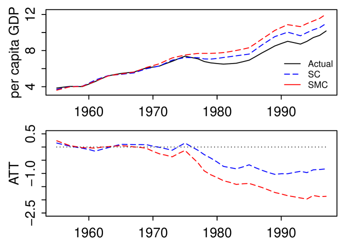
Figure 1: Study of the Basque Country. Left: Actual and counterfactual per capita GDP of the Basque Country. Right: The difference of actual and counterfactual values (ATT).

Table 3: Estimates of weights for alternative estimators in the Basque study. The comprehensive weights $\theta_{j}w_{j}$ and the coefficients are reported for SRC and OLS, respectively.

region	SC	dSC	MASC	OLS	lasso	SRC
Andalucia	0	0	0	0.217	-0.112	0
Aragon	0	0	0	-3.059	0	0
Asturias	0	0	0	1.460	0	0.001
Baleares	0	0.582	0	-0.365	0.365	0
Canarias	0	0	0	-0.245	0	0
Cantabria	0	0	0	0.048	0.048	0.311
Leon	0	0	0	0.080	0	0
Mancha	0	0	0	0.861	0	0
Cataluna	0.851	0	0.851	-0.174	0.174	0.028
Valenciana	0	0	0	1.766	0.065	0
Extremadura	0	0	0	-0.401	0	0
Galicia	0	0	0	-0.396	0	0
Madrid	0.149	0.418	0.149	0.533	0	0.276
Murcia	0	0	0	-0.547	0	0
Navarra	0	0	0	1.302	0.234	0
Rioja	0	0	0	0.673	0	0.587
Intercept	-	-0.335	-	-2.580	1.097	0.047

6 Discussion

This paper makes three contributions: (1) We propose a simple and effective method, Synthetic Regressing Control, by synthesizing the fitted controls. (2) We determine the weights by minimizing the unbiased risk estimate criterion. We demonstrate that this method is asymptotically optimal, achieving the lowest possible squared error. (3) We expand the method in several domains, including conducting inference, extending it to cases where control units is more than time periods, and incorporating auxiliary covariates.

There are several potential directions for future work. First, we focus on the simple linear regression to reduce the issue of imperfect fit. Consequently, the synthesis method relies on the simple linear regression. However, the SRC method may be applicable for more complex data structures, such as discrete, count, or hierarchical outcomes. Therefore, extending the method to broader regression models is an interesting direction. Second, for settings with multiple treated units, we can fit SRC separately for each treated unit, as in Abadie (2021). However, this approach brings a loss of efficiency due to the correlation of treated units. Therefore, efficiently extending the method to multiple treated units is a worthy direction. Third, a set of auxiliary covariates is available, we pool the auxiliary covariates and the outcomes togother to conduct the SRC method. However, this approach may bring extra risk when the linear approximation relation in the covariates is different from that in the outcomes. Therefore, exploring ways to incorporate auxiliary covariates into the SRC method while minimizing such risks is another worthy problem for future research. Finally, extending it to more complicated situations, such as staggered adoption where units take up the treatment at different times (Ben-Michael et al., 2022), is another challenging direction.

Appendix A: Proofs of Results

Proof of Theorem 1

For simplifying the notation, we assume, without loss of generality, that $\mathbf{y}_{j},\forall j=1,\cdots,J+1$ and $\mathbf{\mu}_{1}$ are centered, i.e., $\mathbf{1}^{\top}\mathbf{y}_{j}=0$ and $\mathbf{1}^{\top}\mathbf{\mu}_{1}=0$.

The solution $\hat{\boldsymbol{\theta}}=(\hat{\theta}_{2},\cdots,\hat{\theta}_{J+1})^{\top}$ satisfies:

$$\hat{\boldsymbol{\theta}}= \left[\text{diag}(\mathbf{Y}_{0}^{\top}\mathbf{Y}_{0})\right]^{-1}\mathbf{Y}_{0}^{\top}\mathbf{y}_{1}.$$ (A.1)

Inserting $\hat{\boldsymbol{\theta}}$ into the criterion $\mathcal{C}_{c}({\boldsymbol{w}})$, we have

$$\mathcal{C}_{c}({\boldsymbol{w}}) =\left\|\mathbf{y}_{1}-\mathbf{Y}_{0}\mathbf{W}\left[\text{diag}(\mathbf{Y}_{0}^{\top}\mathbf{Y}_{0})\right]^{-1}\mathbf{Y}_{0}^{\top}\mathbf{y}_{1}\right\|^{2}+2\hat{\sigma}^{2}{\boldsymbol{w}}^{\top}\mathbf{1}.$$ (A.2)

By the above analysis on Algorithm 1, we just need to prove the asymptotic optimality by analyzing (A.2). In the theorem, we have the following conditions:

$$(C1)\quad\max_{t}\mathbb{E}\left[\epsilon_{t}^{4}\right]\leq c_{1}<\infty\text{ for some constant }c_{1}.$$ (A.3)

$$(C2)\quad\|\boldsymbol{\mu}_{1}\|^{2}/T_{0}\leq c_{2}<\infty\text{ for some constant }c_{2}.$$ (A.4)

$$(C3)\quad J^{-1}\|\boldsymbol{\mu}_{1}-\mathbf{Y}_{0}[\text{diag}(\mathbf{Y}_{0}^{\top}\mathbf{Y}_{0})]^{-1}\mathbf{Y}_{0}^{\top}\boldsymbol{\mu}_{1}\|^{2}\rightarrow\infty\text{ as }T_{0}\rightarrow\infty.$$ (A.5)

Let $\mathbf{M}({\boldsymbol{w}})=\mathbf{Y}_{0}\mathbf{W}\left[\text{diag}(\mathbf{Y}_{0}^{\top}\mathbf{Y}_{0})\right]^{-1}\mathbf{Y}_{0}^{\top}$ and ${\bf A}({\boldsymbol{w}})={\bf I}-\mathbf{M}({\boldsymbol{w}})$. We have

$$\hat{\bf y}_{1}({\boldsymbol{w}})=\mathbf{M}({\boldsymbol{w}}){\bf y}_{1},$$ (A.6)

$$L({\boldsymbol{w}})=\|\hat{\bf y}_{1}({\boldsymbol{w}})-\boldsymbol{\mu}_{1}\|^{2}=\|\mathbf{M}({\boldsymbol{w}}){\bf y}_{1}-\boldsymbol{\mu}_{1}\|^{2}.$$ (A.7)

From (A.7), a simple calculation follows

$$R({\boldsymbol{w}})=E\{L({\boldsymbol{w}})\}=\left\|{\bf A}({\boldsymbol{w}})\boldsymbol{\mu}_{1}\right\|^{2}+\hbox{trace}\left\{\mathbf{M}({\boldsymbol{w}}){\bf\Sigma}\mathbf{M}^{\top}({\boldsymbol{w}})\right\}\geq\left\|{\bf A}({\boldsymbol{w}})\boldsymbol{\mu}_{1}\right\|^{2}.$$ (A.8)

Thus, combing (A.8) and Condition (A.5), we have

$$\inf_{w\in\mathcal{H}_{J}}J^{-1}R({\boldsymbol{w}})\rightarrow\infty.$$ (A.9)

Denote ${\bf\Sigma}=\text{diag}\{\sigma_{1}^{2},\cdots,\sigma_{T_{0}}^{2}\}$. From (A.2) and (A.7), we have

$$\mathcal{C}_{c}({\boldsymbol{w}})-L({\boldsymbol{w}}) =\|\hat{\bf y}_{1}({\boldsymbol{w}})-\boldsymbol{\mu}_{1}-{\boldsymbol{\epsilon}}\|^{2}+2\hat{\sigma}^{2}{\boldsymbol{w}}^{\top}\mathbf{1}-\left\|\mathbf{M}({\boldsymbol{w}}){\bf y}_{1}-\boldsymbol{\mu}_{1}\right\|^{2}$$

$$=-2\left\{\hat{\bf y}_{1}({\boldsymbol{w}})-\boldsymbol{\mu}_{1}\right\}^{\top}{\boldsymbol{\epsilon}}+2\hat{\sigma}^{2}{\boldsymbol{w}}^{\top}\mathbf{1}+\left\|{\boldsymbol{\epsilon}}\right\|^{2}$$

$$=-2{\boldsymbol{\epsilon}}^{\top}\mathbf{M}({\boldsymbol{w}}){\bf y}_{1}+2\hat{\sigma}^{2}{\boldsymbol{w}}^{\top}\mathbf{1}+2\boldsymbol{\mu}_{1}^{\top}{\boldsymbol{\epsilon}}+\left\|{\boldsymbol{\epsilon}}\right\|^{2}$$

$$=-2{\boldsymbol{\epsilon}}^{\top}\mathbf{M}({\boldsymbol{w}})\boldsymbol{\mu}_{1}-2{\boldsymbol{\epsilon}}^{\top}\mathbf{M}({\boldsymbol{w}}){\boldsymbol{\epsilon}}+2\hat{\sigma}^{2}{\boldsymbol{w}}^{\top}\mathbf{1}+2\boldsymbol{\mu}_{1}^{\top}{\boldsymbol{\epsilon}}+\left\|{\boldsymbol{\epsilon}}\right\|^{2},$$ (A.10)

where the last three terms in the last line do not involve ${\boldsymbol{w}}$. From (A.7) and (A.8), we have

$$R({\boldsymbol{w}})-L({\boldsymbol{w}})= \left\|{\bf A}({\boldsymbol{w}})\boldsymbol{\mu}_{1}\right\|^{2}+\hbox{trace}\left\{\mathbf{M}({\boldsymbol{w}}){\bf\Sigma}\mathbf{M}^{\top}({\boldsymbol{w}})\right\}-\left\|\mathbf{M}({\boldsymbol{w}}){\bf y}_{1}-\boldsymbol{\mu}_{1}\right\|^{2}$$

$$= \left\|{\bf A}({\boldsymbol{w}})\boldsymbol{\mu}_{1}\right\|^{2}+\hbox{trace}\left\{\mathbf{M}({\boldsymbol{w}}){\bf\Sigma}\mathbf{M}^{\top}({\boldsymbol{w}})\right\}-\left\|{\bf A}({\boldsymbol{w}})\boldsymbol{\mu}_{1}-\mathbf{M}({\boldsymbol{w}}){\boldsymbol{\epsilon}}\right\|^{2}$$

$$= -\left\|\mathbf{M}({\boldsymbol{w}}){\boldsymbol{\epsilon}}\right\|^{2}+\hbox{trace}\left\{\mathbf{M}({\boldsymbol{w}}){\bf\Sigma}\mathbf{M}^{\top}({\boldsymbol{w}})\right\}+2{\boldsymbol{\epsilon}}^{\top}\mathbf{M}({\boldsymbol{w}}){\bf A}({\boldsymbol{w}})\boldsymbol{\mu}_{1}.$$ (A.11)

Thus, to prove the asymptotic optimality, We need only to verify that

$$\begin{array}[]{lll}&(\text{i})\ \sup\limits_{{\boldsymbol{w}}\in{\cal H}_{J}}R^{-1}({\boldsymbol{w}})\left|{\boldsymbol{\epsilon}}^{\top}\mathbf{M}({\boldsymbol{w}})\boldsymbol{\mu}_{1}\right|=o_{P}(1),\\ &(\text{ii})\ \sup\limits_{{\boldsymbol{w}}\in{\cal H}_{J}}R^{-1}({\boldsymbol{w}})[\hat{\sigma}^{2}{\boldsymbol{w}}^{\top}\mathbf{1}-{\boldsymbol{\epsilon}}^{\top}\mathbf{M}({\boldsymbol{w}}){\boldsymbol{\epsilon}}]=o_{P}(1),\\ &(\text{iii})\ \sup\limits_{{\boldsymbol{w}}\in{\cal H}_{J}}R^{-1}({\boldsymbol{w}})\left\|\mathbf{M}({\boldsymbol{w}}){\boldsymbol{\epsilon}}\right\|^{2}=o_{P}(1),\\ &(\text{iv})\ \sup\limits_{{\boldsymbol{w}}\in{\cal H}_{J}}R^{-1}({\boldsymbol{w}})\hbox{trace}\left\{\mathbf{M}({\boldsymbol{w}}){\bf\Sigma}\mathbf{M}^{\top}({\boldsymbol{w}})\right\}=o_{P}(1),\\ &(\text{v})\ \sup\limits_{{\boldsymbol{w}}\in{\cal H}_{J}}R^{-1}({\boldsymbol{w}})\left|{\boldsymbol{\epsilon}}^{\top}\mathbf{M}({\boldsymbol{w}}){\bf A}({\boldsymbol{w}})\boldsymbol{\mu}_{1}\right|=o_{P}(1).\end{array}$$

Let $\mathbf{H}=\mathbf{Y}_{0}\left[\text{diag}(\mathbf{Y}_{0}^{\top}\mathbf{Y}_{0})\right]^{-1}\mathbf{Y}_{0}^{\top}$. A direct simplification yields

$$\mathbf{M}({\boldsymbol{w}}) \leq\mathbf{H},$$ (A.12)

where the inequality is in Loewner ordering. Given Condition (A.3), applying Theorem 2 of Whittle (1960) leads to that, for some constant $0<\eta<\infty$,

$$\mathbb{E}\left[\left({\boldsymbol{\epsilon}}^{\top}\mathbf{H}{\boldsymbol{\epsilon}}-\mathbb{E}\left[{\boldsymbol{\epsilon}}^{\top}\mathbf{H}{\boldsymbol{\epsilon}}\right]\right)^{2}\right]\leq\eta(\hbox{trace}\{\mathbf{H}{\bf\Sigma}\mathbf{H}({\boldsymbol{w}})\}).$$ (A.13)

Thus, we have

$$\mathbf{\epsilon}^{\top}\mathbf{H}\mathbf{\epsilon}= E(\mathbf{\epsilon}^{\top}\mathbf{H}\mathbf{\epsilon})+O_{P}\bigg{\{}\sqrt{Var(\mathbf{\epsilon}^{\top}\mathbf{H}\mathbf{\epsilon})}\bigg{\}}$$

$$= \hbox{trace}\{{\bf\Sigma}\mathbf{H}\}+O_{P}\bigg{\{}\sqrt{\hbox{trace}\{{\bf\Sigma}\mathbf{H}\}}\bigg{\}}$$

$$= O_{p}(J).$$ (A.14)

From (A.9) and (Appendix A: Proofs of Results), we have

$$\sup\limits_{{\boldsymbol{w}}\in{\cal H}_{J}}\frac{{\boldsymbol{\epsilon}}^{\top}\mathbf{H}{\boldsymbol{\epsilon}}}{R({\boldsymbol{w}})}\leq\frac{O_{P}(J)}{R({\boldsymbol{w}})}=o_{P}(1).$$ (A.15)

From (A.9) and (A.15), we have

$$\sup\limits_{{\boldsymbol{w}}\in{\cal H}_{J}}\frac{\left|{\boldsymbol{\epsilon}}^{\top}\mathbf{H}\mathbf{A}({\boldsymbol{w}})\boldsymbol{\mu}_{1}\right|}{R({\boldsymbol{w}})}\leq\sup\limits_{{\boldsymbol{w}}\in{\cal H}_{J}}\frac{\left\|\mathbf{H}{\boldsymbol{\epsilon}}\right\|\left\|{\bf A}({\boldsymbol{w}})\boldsymbol{\mu}_{1}\right\|}{R({\boldsymbol{w}})}\leq\sup\limits_{{\boldsymbol{w}}\in{\cal H}_{J}}\frac{\left\|\mathbf{H}{\boldsymbol{\epsilon}}\right\|}{R^{1/2}({\boldsymbol{w}})}=o_{P}(1).$$

Thus, (i) is proved.

From Condition (A.4), we have

$$\hat{\sigma}^{2}=\frac{\|\mathbf{y}_{1}-\mathbf{Y}_{0}(\mathbf{Y}_{0}^{\top}\mathbf{Y}_{0})^{-1}\mathbf{Y}_{0}^{\top}\mathbf{y}_{1}\|^{2}}{T_{0}-J}=O_{P}(1).$$ (A.16)

It follows that

$$\sup\limits_{{\boldsymbol{w}}\in{\cal H}_{J}}\frac{|\hat{\sigma}^{2}{\boldsymbol{w}}^{\top}\mathbf{1}-{\boldsymbol{\epsilon}}^{\top}\mathbf{M}({\boldsymbol{w}}){\boldsymbol{\epsilon}}|}{R({\boldsymbol{w}})}\leq\sup\limits_{{\boldsymbol{w}}\in{\cal H}_{J}}\frac{\hat{\sigma}^{2}{\boldsymbol{w}}^{\top}\mathbf{1}}{R({\boldsymbol{w}})}+\sup\limits_{{\boldsymbol{w}}\in{\cal H}_{J}}\frac{{\boldsymbol{\epsilon}}^{\top}\mathbf{H}{\boldsymbol{\epsilon}}}{R({\boldsymbol{w}})}=o_{P}(1),$$

where the last step is from (A.9), (A.15), and (A.16). Thus, (ii) is proved.

From (A.12), we have

$$\sup\limits_{{\boldsymbol{w}}\in{\cal H}_{J}}\frac{\|\mathbf{M}({\boldsymbol{w}}){\boldsymbol{\epsilon}}\|^{2}}{R({\boldsymbol{w}})}\leq\sup\limits_{{\boldsymbol{w}}\in{\cal H}_{J}}\frac{{\boldsymbol{\epsilon}}^{\top}\mathbf{H}{\boldsymbol{\epsilon}}}{R({\boldsymbol{w}})}=o_{P}(1),$$

where the last step is from (A.9). Thus, (iii) is proved.

From (A.12), we have

$$\sup\limits_{{\boldsymbol{w}}\in{\cal H}_{J}}\frac{\hbox{trace}\left\{\mathbf{M}({\boldsymbol{w}}){\bf\Sigma}\mathbf{M}^{\top}({\boldsymbol{w}})\right\}}{R({\boldsymbol{w}})}\leq\sup\limits_{{\boldsymbol{w}}\in{\cal H}_{J}}\frac{\hbox{trace}\{\mathbf{H}{\bf\Sigma}\}}{R({\boldsymbol{w}})}=o_{P}(1),$$

where the last step is from (A.9) and Condition (A.3). Thus, (iv) is proved.

From (A.8) and (A.12), we have

$$\sup\limits_{{\boldsymbol{w}}\in{\cal H}_{J}}\frac{\left|{\boldsymbol{\epsilon}}^{\top}\mathbf{M}({\boldsymbol{w}}){\bf A}({\boldsymbol{w}})\boldsymbol{\mu}_{1}\right|}{R({\boldsymbol{w}})}\leq\sup\limits_{{\boldsymbol{w}}\in{\cal H}_{J}}\frac{\left\|\mathbf{M}({\boldsymbol{w}}){\boldsymbol{\epsilon}}\right\|\left\|{\bf A}({\boldsymbol{w}})\boldsymbol{\mu}_{1}\right\|}{R({\boldsymbol{w}})}\leq\sup\limits_{{\boldsymbol{w}}\in{\cal H}_{J}}\frac{\left\|\mathbf{H}{\boldsymbol{\epsilon}}\right\|}{R^{1/2}({\boldsymbol{w}})}=o_{P}(1),$$

where the last step is from (A.15). It means that (vi) is proved. Therefore, the theorem is proved.

$\square$

References

- Abadie (2021) Abadie, A. (2021). Using synthetic controls: Feasibility, data requirements, and methodological aspects. Journal of Economic Literature 59, 391–425.
- Abadie et al. (2010) Abadie, A., A. Diamond, and J. Hainmueller (2010). Synthetic control methods for comparative case studies: Estimating the effect of cali- fornia’s tobacco control program. Journal of the American Statistical Association 105(490), 493–505.
- Abadie et al. (2015) Abadie, A., A. Diamond, and J. Hainmueller (2015). Comparative politics and the synthetic control method. American Journal of Political Science 59, 495–510.
- Abadie and Gardeazabal (2003) Abadie, A. and J. Gardeazabal (2003). The economic costs of conflict: A case study of the basque country. The American Economic Review 93, 113–132.
- Abadie and L’Hour (2021) Abadie, A. and J. L’Hour (2021). A penalized synthetic control estimator for disaggregated data. Journal of the American Statistical Association 536(116), 1817–1834.
- Amjad et al. (2018) Amjad, M., D. Shah, and D. Shen (2018). Robust synthetic control. The Journal of Machine Learning Research 19, 802–852.
- Arkhangelsky et al. (2021) Arkhangelsky, D., S. Athey, D. A. Hirshberg, G. W. Imbens, and S. Wager (2021). Synthetic difference in differences. American Economic Review 111, 4088–4118.
- Athey et al. (2021) Athey, S., M. Bayati, N. Doudchenko, G. Imbens, and K. Khosravi (2021). Matrix completion methods for causal panel data models. Journal of the American Statistical Association 116(536), 1716–1730.
- Athey et al. (2019) Athey, S., M. Bayati, G. Imbens, and Z. Qu (2019). Ensemble methods for causal effects in panel data settings. AEA Papers and Proceedings 109, 65–70.
- Ben-Michael et al. (2021) Ben-Michael, E., A. Feller, and J. othstein (2021). The augmented synthetic control method. Journal of the American Statistical Association 536(116), 1789–1803.
- Ben-Michael et al. (2022) Ben-Michael, E., A. Feller, and J. Rothstein (2022). Synthetic controls with staggered adoption. Journal of the Royal Statistical Society, Series B 84, 351–381.
- Chernozhukov et al. (2021) Chernozhukov, V., K. Wüthrich, and Y. Zhu (2021). An exact and robust conformal inference method for counterfactual and synthetic controls. Journal of the American Statistical Association 536(116), 1849–1864.
- Doudchenko and Imbens (2016) Doudchenko, N. and G. W. Imbens (2016, October). Balancing, regression, difference-in-differences and synthetic control methods: A synthesis. Working Paper 22791, National Bureau of Economic Research.
- Fan and Lv (2008) Fan, J. and J. Lv (2008). Sure independence screening for ultrahigh dimensional feature space (with discussion). Journal of the Royal Statistical Society, Series B 70, 849–911.
- Ferman and Pinto (2021) Ferman, B. and C. Pinto (2021). Synthetic controls with imperfect pretreatment fit. Quantitative Economics 12, 1197–1221.
- Gobillon and Magnac (2016) Gobillon, L. and T. Magnac (2016). Regional policy evaluation: Inter- active fixed effects and synthetic controls. Review of Economics and Statistics 98, 535–551.
- Hansen (2007) Hansen, B. (2007). Least squares model averaging. Econometrica 75, 1175–1189.
- Hsiao et al. (2012) Hsiao, C., S. Ching, and K. Wan (2012). A panel data approach for program evaluation: Measuring the benefits of political and economic integration of hong kong with mainland china. Journal of Applied Econometrics 27, 705–740.
- Kellogg et al. (2021) Kellogg, M., M. Mogstad, G. Guillaume A. Pouliot, and A. Torgovitsky (2021). Combining matching and synthetic control to tradeoff biases from extrapolation and interpolation. Journal of the American Statistical Association 536(116), 1804–1814.
- Li (2020) Li, K. (2020). Statistical inference for average treatment effects estimated by synthetic control methods. Journal of the American Statistical Association 115(532), 2068–2083.
- Li (1987) Li, K.-C. (1987). Asymptotic optimality for , , cross-validation and generalized cross-validation: Discrete index set. The Annals of Statistics 15, 958–975.
- Powell (2018) Powell, D. (2018, May). Imperfect synthetic controls: Did the massachusetts health care reform save lives? Technical report, Santa Monica, CA: RAND Corporation.
- Robbins et al. (2017) Robbins, M., J. Saunders, and B. Kilmer (2017). A framework for synthetic control methods with high-dimensional, micro-level data: Evaluating a neighborhood-specific crime intervention. Journal of the American Statistical Association 112, 109–126.
- Viviano and Bradic (2023) Viviano, D. and J. Bradic (2023). Synthetic learner: Model-free inference on treatments over time. Journal of Econometrics 234(2), 691–713.
- Whittle (1960) Whittle, P. (1960). Bounds for the moments of linear and quadratic forms in independent variables. Theory of Probability and its Applications 5(3), 302–305.
- Xu (2017) Xu, Y. (2017). Generalized synthetic control method: Causal inference with interactive fixed effects models. Political Analysis 25, 57–76.
- Zhu et al. (2011) Zhu, L., L. Li, R. Li, and L. Zhu (2011). Model-free feature screening for ultrahigh-dimensional data. Journal of the American Statistical Association 106, 1464–1475.