Latent Optimal Paths by Gumbel Propagation for Variational Bayesian Dynamic Programming

Abstract

We propose a unified approach to obtain structured sparse optimal paths in the latent space of a variational autoencoder (VAE) using dynamic programming and Gumbel propagation. We solve the classical optimal path problem by a probability softening solution, called the stochastic optimal path, and transform a wide range of DP problems into directed acyclic graphs in which all possible paths follow a Gibbs distribution. We show the equivalence of the Gibbs distribution to a message-passing algorithm by the properties of the Gumbel distribution and give all the ingredients required for variational Bayesian inference. Our approach obtaining latent optimal paths enables end-to-end training for generative tasks in which models rely on the information of unobserved structural features. We validate the behavior of our approach and showcase its applicability in two real-world applications: text-to-speech and singing voice synthesis. https://github.com/Berthaniu/LatentOptimalPathsBayesianDP

1 Introduction

Optimal paths are often required in generative tasks such as speech, music, and language modeling [1, 2, 3]. These tasks involve the simultaneous identification of structured relationships between data and conditions. Obtaining optimal paths given a graph with edge weights enables models to achieve an improved fit based on extracted unobserved structural features. The optimal paths problem can be solved by dynamic programming (DP) which breaks the problem down into several sub-problems and finds optimal solutions within the sub-problems iteratively.

Since the DP algorithm finds optimal paths using the max operator, it is non-differentiable which limits the usage of the DP algorithm in neural networks where gradient back-propagation is applied. As a workaround, previous works have approximated the max operator with smoothed functions to allow differentiation of DP algorithms [4]. However, smoothed approximations of DP lose the sparsity of solutions which makes hard assignments become soft assignments. Alternatively, some works [5, 6, 7, 2, 8, 9, 10, 11] split the training strategies in which models depend on sparse outputs from external DP aligners [12, 13] or pre-trained models [14]. These external components involve more than one training phase thus the model performance critically relies on them.

In this work, we explore a novel method to obtain structured sparse optimal paths in the latent space of variational autoencoders (VAEs) by DP. Instead of a smoothed approximation, we propose the stochastic optimal path solution, which is a probabilistic softening solution by defining a Gibbs distribution where the energy function is the path score. We show this to be equivalent to a message-passing algorithm on the directed acyclic graphs (DAG) using the max and shift properties of the Gumbel distribution. To learn the latent optimal paths, we give tractable ingredients for variational Bayesian inference (i.e., likelihood and KL divergence) using DP, namely Bayesian dynamic programming (BDP), which enables VAEs to obtain latent optimal paths within a DAG and achieve end-to-end training on generative tasks that rely on sparse unobserved structural relationships.

We make the following contributions: (1) We present a unified framework that gives a probabilistic softening of the classical optimal path problem on DAGs. We notably give efficient algorithms in linear time for sampling, computing the likelihood, and computing the KL divergence, thereby providing all of the ingredients required for variational Bayesian inference with a latent optimal path. (2) We introduce a conditional BDP-VAE framework which learns sparse latent optimal path. Since the data information is not observed during inference, it is difficult to form the distribution statistics (i.e., edge weights) in the prior encoder. We give an alternative and flexible method to form the distribution statistics on the conditional prior by making use of a flow-based model. (3) We demonstrate how the BDP-VAE framework achieves end-to-end training with latent monotonic alignment (MA) paths on the text-to-speech (TTS) task and singing voice synthesis (SVS) task, and verify the proposed latent optimal paths on the computational graph of dynamic time warping (DTW).

2 Related Work

We present a new VAE [15] framework learning sparse latent optimal path by DP with Gumbel propagation. Since traditional DP is non-differentiable, there exist many alternative works that integrate dynamic programming into the neural networks by involving a convex optimization problem [16, 17]. Instead, [18] proposed a unified DP framework by turning a broad class of DP problems into a DAG and obtaining the optimal path by a max operator smoothed with a strongly convex regularizer. This work can be applied in structured prediction tasks [19] under a supervised framework. Graphical models such as Bayesian networks [20] learn dependencies of random variables based on a DAG, our method treats the paths of a DAG, not the nodes, as random variables of a Gibbs distribution.

In many conditional generative tasks, models usually rely on dependencies of data and conditions, in which these dependencies are unobserved. [6, 11, 10] use a multiple training strategy by obtaining the sparse dependencies from an external DP-based techniques [12] at first, then use the outputs as additional inputs to the model. Glow-TTS [1] integrates the a DP algorithm on a flow-based model [1] to obtain unobserved monotonic alignment in parallel. Other models with structured latent representations such as HMMs [21] and PCFGs [22] make strong assumptions about the model structure which could limit their flexibility and applicability. Instead, we propose a unified framework to enable the VAEs to capture sparse latent optimal paths, allowing for flexible adaptation to a variety of tasks.

Attention mechanisms are an alternative solution which is also widely applied for obtaining structured features in many seq-to-seq generative tasks. Compared to DP, attention mechanisms can be computationally expensive, especially for large input sequences. The MoChA [23] reduces the computational complexity by involving a DP. Our work uses DP to obtain latent optimal paths and we show that this occurs in linear time (Corollary 4.11). Due to the gradient propagation, previous works with attentions such as [24, 25, 26] cannot achieve hard alignment during training. LAVA [27] makes use of the properties of VAEs [15] and captures the unobserved alignment by proposing learning latent alignment with attention on VAEs. To obtain a structural constraint (i.e., monotonic alignment) attention strongly relies on model structures and DP to extract marginalization of the attention alignment distribution [28, 29]. Instead, we defined a path distribution given a DAG with edge weights and perform variational Bayesian inference by DP. By capturing unobserved sparse optimal trajectories under the defined DAG in VAEs’ latent space, our approach facilitates the development of more explicit structural unobserved representations for a variety of applications.

The Gumbel-Max trick makes use of the max property of the Gumbel distribution which allows for efficient sampling from discrete distributions [30]. [31, 32] facilitate gradient-based learning for Gibbs distribution by relaxing the component-wise optimization in the Gumbel-Max trick. [33] focuses on leveraging the Gumbel-Max trick on the score function estimator. Unlike those works, our research leverages the max and shift properties of Gumbel distribution for message-passing on DP to enable sparse structural latent representation learning in VAEs. We provide ingredients required for variational Bayesian inference, in which training relies on a score-based estimator.

3 Definitions and Mathematical Background

This section provides background on the notation definition of a DAG, a definition of the traditional optimal path problem given a DAG, and properties of the Gumbel random variable.

Definition of a Graph: We denote $\mathcal{R}=(\mathcal{V},\mathcal{E})$ be a directed acyclic graph with nodes $\mathcal{V}$ and edges $\mathcal{E}$. Assume without loss of generality that the nodes are numbered in topological order, such that $\mathcal{V}=(1,2,\dots,N)$ and $u<v$ for all $(u,v)\in\mathcal{E}$. Further, we assume that $1$ is the only node without parents and $N$ the only node without children. We denote the edge weights $\mathbf{W}\in\mathbb{R}^{N\times N}$ with $w_{i,j}=-\infty$ for all $(u,v)\not\in\mathcal{E}$. Let $\mathcal{Y}(1,v)$ be the set of all paths from $1$ to $v$. Associate with each path $\mathbf{y}=(y_{1},y_{2},\dots,y_{|{\mathbf{y}}|})$ a score obtained by summing edge weights along the path, defined as $||\mathbf{y}||_{\mathbf{W}}=\sum_{i=2}^{|{\mathbf{y}}|}w_{y_{i-1},y_{i}}=\sum_{(u,v)\in\mathbf{y}}w_{u,v}$, where the final expression introduces the notation $(u,v)\in\mathbf{y}$ for the edges $(u,v)$ that make up path $\mathbf{y}$. Denote the set of parents of node $v$ by $\mathcal{P}(v)=\{u:(u,v)\in\mathcal{E}\}$ and the set of children of node $u$ by $\mathcal{C}(u)=\{v:(u,v)\in\mathcal{E}\}$.

Non-Stochastic Optimal Paths: The traditional optimal path problem is to find the highest scoring path from node $1$ to node $N$,

$$\mathbf{y}^{*}=\operatorname*{\arg\!\max}_{\mathbf{y}\in\mathcal{Y}(1,N)}||\mathbf{y}||_{\mathbf{W}}.$$ (1)

This can be solved in $O(\left|\mathcal{E}\right|)$ time by iterating in topological order. The score $\xi(\cdot)$ is defined as

$$\xi(1) =0$$ (2)

$$\forall v\in\left\{2,3,\dots,N\right\},~{}~{}~{}\xi(v) =\max_{u\in\mathcal{P}(v)}\xi(u)+w_{u,v},$$ (3)

after which $\mathbf{y}^{*}$ is obtained (in reverse) by tracing from $N$ to $1$, following the path of nodes $u$ for which the maximum was obtained in the above.

Gumbel Random Variable: Let $\mathcal{G}(\mu)$ denote the unit scale Gumbel random variable with location parameter $\mu$ and probability density function

$$\mathcal{G}(x|\mu)=\exp(-(x-\mu)-\exp(x-\mu)).$$ (4)

We now review the properties of the Gumbel which we will exploit in Section 4. Let $X\sim\mathcal{G}(\mu)$. The Gumbel distribution is closed under shifting, with

$$X+\mathrm{const.} \sim\mathcal{G}(\mu+\mathrm{const.}).$$ (5)

Let $X_{i}\sim\mathcal{G}(\mu_{i})$ for all $i\in\left\{1,2,\dots,m\right\}$. The Gumbel is also closed under the $\max$ operation, with

$$\max(\left\{X_{1},X_{2},\dots,X_{m}\right\})\sim\mathcal{G}(\log\sum_{i=1}^{m}\exp(\mu_{i})).$$ (6)

Finally, there is a closed-form expression for the index which obtains the maximum in the above expression, namely

$$p(k=\operatorname*{\arg\!\max}_{i\in\{1,2,\dots,m\}}X_{i})=\frac{\exp(\mu_{k})}{\sum_{i=1}^{m}\exp(\mu_{i})}.$$ (7)

4 Bayesian Dynamic Programming

In this section, we propose a stochastic approach to seek optimal paths. We denote a distribution family given a DAG with edge weights and give ingredients required for variational Bayesian inference by using DP with Gumbel propagation, namely, Bayesian dynamic programming .

4.1 Stochastic Optimal Paths

In the stochastic approach, every possible path $\mathbf{y}\in\mathcal{Y}$ on $\mathbf{W}$ follows a Gibbs distribution given a DAG $\mathcal{R}$, edge weights $\mathbf{W}$ and temperature parameter $\alpha$ defined by Definition 4.1.

Definition 4.1.

Denote by

$$\mathcal{D}(\mathcal{R},\mathbf{W},\alpha)$$ (8)

the Gibbs distribution over $\mathbf{y}\in\mathcal{Y}(1,N)$ with probability mass function

$$\mathcal{D}(\mathbf{y}|\mathcal{R},\mathbf{W},\alpha) =\frac{\exp(\alpha\left\|\mathbf{y}\right\|_{\mathbf{W}})}{\sum_{\widehat{\mathbf{y}}\in\mathcal{Y}(1,N)}\exp(\alpha\left\|\widehat{\mathbf{y}}\right\|_{\mathbf{W}})}.$$ (9)

Despite the intractable form of the denominator in Equation 9, we provide the ingredients necessary for approximate Bayesian inference for latent distribution (unobserved) $\mathcal{D}$. In particular, we can efficiently compute the normalized likelihood (Corollary 4.6), sample (Corollary 4.7), and compute the KL divergence within $\mathcal{D}(\mathcal{R},\cdot,\alpha)$ (Lemma 4.10) in linear time (Corollary 4.11).

4.2 Gumbel Propagation

The Gumbel propagation offers an equivalent formulation of Definition 4.1 that lends itself to dynamic programming by the properties in Equation 7 and Equation 5 as per the following result.

Lemma 4.2.

Let

$$Y=\operatorname*{\arg\!\max}_{\mathbf{y}\in\mathcal{Y}(1,N)}\left\{\Omega_{\mathbf{y}}\right\},$$ (10)

where for all $\mathbf{y}\in\mathcal{Y}(1,N)$,

$$\Omega_{\mathbf{y}} =\mathcal{\alpha}\left\|\mathbf{y}\right\|_{\mathbf{W}}+G_{\mathbf{y}}$$ (11)

$$G_{\mathbf{y}} \sim\mathcal{G}(0).$$ (12)

Then the probability of $Y=\mathbf{y}$ is given by (9).

Let the definitions of $\Omega_{\mathbf{y}}$ and $G_{\mathbf{y}}$ extend to all $\mathbf{y}\in\bigcup_{u=1}^{N}\mathcal{Y}(1,u)$, which is the set of all partial paths. We define for each node $v\in\mathcal{V}$ the real-valued random variable

$$Q_{v} =\max_{\mathbf{y}\in\mathcal{Y}(1,v)}\left\{\Omega_{\mathbf{y}}\right\}.$$ (13)

Lemma 4.3.

The $Q_{v}$ are Gumbel distributed with

$$Q_{v}\sim\mathcal{G}(\mu_{v}),$$ (14)

where

$$\mu_{v}=\log\sum_{\mathbf{y}\in\mathcal{Y}(1,v)}\exp(\alpha\left\|\mathbf{y}\right\|_{\mathbf{W}}).$$ (15)

We now state the first main result in Lemma 4.4.

Lemma 4.4.

The location parameters $\mu_{v}$ satisfy the recursion

$$\mu_{1} =0$$ (16)

$$\mu_{v} =\log\sum_{u\in\mathcal{P}(v)}\exp(\mu_{u}+\alpha\,w_{u,v}).$$ (17)

for all $v\in\left\{2,3,\dots,N\right\}$.

4.3 Sampling and Likelihood

Then we state an alternative normalized likelihood of a sampled path $\mathbf{y}$ by Corollary 4.7 as Corollary 4.6 according to a transition matrix defined in Lemma 4.5. The transition matrix in Lemma 4.5 can be computed according to the location parameter $\mu$ defined in Lemma 4.4 directly.

Lemma 4.5.

Let $\mathbf{y}=(y_{1},y_{2},\dots,y_{\left|\mathbf{y}\right|})\sim Y$, where the random variable $Y$ is defined in (10). The probability of the transition $v\rightarrow u$ is

$$\pi_{u,v} \equiv p(y_{i-1}=u|y_{i}=v,u\in\mathcal{P}(v))$$ (18)

$$=\frac{\exp(\mu_{u}+\alpha\,w_{u,v})}{\exp(\mu_{v})},$$ (19)

for all $i\in\{2,3,\dots,N\}$.

Corollary 4.6.

The path probability may be written

$$\mathcal{D}(\mathbf{y}|\mathcal{R},\mathbf{W},\alpha)=\prod_{(u,v)\in\mathbf{y}}\pi_{u,v}.$$ (20)

Corollary 4.7.

Paths $\mathbf{y}\sim\mathcal{D}(\mathcal{R},\mathbf{W},\alpha)$ may be sampled (in reverse) by

1. initializing $v=N$,

2. sampling $u\in\mathcal{P}(v)$ with probability $\pi_{u,v}$,

3. setting $v\leftarrow u$,

4. if $v=1$ then stop, otherwise return to step 2.

4.4 KL Divergence

Given two distributions $\mathcal{D}(\mathcal{R},\mathbf{W},\alpha)$ and $\mathcal{D}(\mathcal{R},\mathbf{W}^{(r)},\alpha)$, we give a tractable closed-form of the KL divergence within the two distributions in Lemma 4.10.

Definition 4.8.

We denote the total probability of paths that include a given edge $(u,v)\in\mathcal{E}$ by

$$\omega_{u,v}\equiv\sum_{\{\mathbf{y}\in\mathcal{Y}(1,N):(u,v)\in\mathbf{y}\}}\mathcal{D}(\mathbf{y}|\mathcal{R},\mathbf{W},\alpha).$$ (21)

The quantity in the above definition may be computed using two dynamic programming passes, one topologically ordered and the other reverse topologically ordered, by applying the following

Lemma 4.9.

For all $(u,v)\in\mathcal{E}$,

$$\omega_{u,v}=\pi_{u,v}\,\lambda_{u}\,\rho_{v},$$ (22)

where we have the recursions

$$\lambda_{1} =1$$ (23)

$$\lambda_{v} =\sum_{u\in\mathcal{P}(v)}\lambda_{u}\,\pi_{u,v}$$ (24)

for all $v\in\left\{2,3,\dots,N\right\}$ (in topological order w.r.t. $\mathcal{R}$), and

$$\rho_{N} =1$$ (25)

$$\rho_{u} =\sum_{v\in\mathcal{C}(u)}\rho_{v}\pi_{u,v}$$ (26)

for all $u\in\left\{N-1,N-2,\dots,1\right\}$ (in reverse topological order w.r.t. $\mathcal{R}$).

Lemma 4.10.

The KL divergence within the family $\mathcal{D}(\mathcal{R},\cdot,\alpha)$ is

$$\mathcal{D}_{\mathrm{KL}}\left[\mathcal{D}(\mathcal{R},\mathbf{W},\alpha)\big{\|}\mathcal{D}(\mathcal{R},\mathbf{W}^{(r)},\alpha)\right]=\mu_{N}^{(r)}-\mu_{N}+\alpha\sum_{(u,v)\in\mathcal{E}}\omega_{u,v}\big{(}w_{u,v}-w_{u,v}^{(r)}\big{)},$$ (27)

where $\omega_{u,v}$ is the marginal probability of edge $(u,v)$ on $\mathcal{D}(\mathcal{R},\mathbf{W},\alpha)$ defined in Definition 4.8, $\mu_{N}$ is defined in Equation 15 and $\mu_{N}^{(r)}$ is similar to $\mu_{N}$ but defined in terms of $\mathbf{W}^{(r)}$ rather than $\mathbf{W}$.

Corollary 4.11.

Both the KL divergence (27) and the likelihood (20) may be computed in $O(\left|\mathcal{E}\right|)$ time.

5 BDP-VAE

We now show how to apply the method in Section 4 to a conditional VAE framework to obtain sparse latent optimal paths. An unconditional BDP-VAE framework can be directly applied based on Corollary 4.6, Corollary 4.7, and Lemma 4.10, but a conditional BDP-VAE framework may be challenging in real applications. Given a sequential input $\mathbf{x}$ with length $t$ and a sequential condition $\mathbf{c}$ with length $n$, where $t\neq n$ and $\{t,n\}$ are varying within the dataset. We wish to find an unobserved structural relationship between $\mathbf{x}$ and $\mathbf{c}$ in the latent space of VAEs denoted as $\mathbf{y}$. Conditional BDP-VAEs consist of three parts: an encoder models posterior distribution $q(\mathbf{y}|\mathbf{x},\mathbf{c};\phi)$, a decoder models the distribution of $p(\mathbf{x}|\mathbf{y},\mathbf{c};\theta)$, and a prior encoder models the prior distribution $p(\mathbf{y}|\mathbf{c};\theta)$.

We assume the conditional input $\mathbf{c}$ is always observed and the conditional ELBO is defined as

$$\mathcal{L}(\phi,\theta,\mathbf{x}|\mathbf{c})=\mathbb{E}_{\mathbf{y}\sim q(\cdot|\mathbf{x},\mathbf{c};\phi)}\log p(\mathbf{x}|\mathbf{y},\mathbf{c};\theta)-\mathcal{D}_{\mathrm{KL}}\left[q(\mathbf{y}|\mathbf{x},\mathbf{c};\phi)\big{\|}p(\mathbf{y}|\mathbf{c};\theta)\right].$$ (28)

5.1 Posterior And Latent Optimal Paths

Given a DAG $\mathcal{R}$ with edge $\mathcal{E}$ and nodes $\mathcal{V}$, the distribution of the posterior encoder is denoted as

$$q(\mathbf{y}|\mathbf{x},\mathbf{c};\phi)=\mathcal{D}(\mathbf{y}|\mathcal{R},\mathbf{W}=\text{NN}_{\mathbf{W}}(\mathbf{x},\mathbf{c};\phi),\alpha)$$ (29)

where NN${}_{\mathbf{W}}(\cdot;\phi)$ is a neural network to obtain the edge weights $\mathbf{W}$ of the DAG $\mathcal{R}$ and $\alpha$ is a preset hyper-parameter. The latent optimal path $\mathbf{y}$ with $\{0,1\}$ only can be sampled according to Lemma 4.4, Lemma 4.5, and Corollary 4.7.

5.2 Conditional Prior

Denote the distribution of the conditional prior as

$$p(\mathbf{y}|\mathbf{c};\theta)=\mathcal{D}(\mathbf{y}|\mathcal{R},\mathbf{W}^{(0)}=\text{NN}_{\mathbf{W^{(0)}}}(\mathbf{c};\theta),\alpha)$$ (30)

We have provided a closed-form KL divergence within the family $\mathcal{D}(\mathcal{R},\cdot,\alpha)$ in Lemma 4.10 which may be convenient for unconditional generation by pre-setting the prior distribution statistics directly. In most conditional generation tasks, the non-accessible $\mathbf{x}$ in real applications leads to problems on the prior encoder when forming the edge weight $\mathbf{W}^{(0)}$ given $\mathbf{c}$ only, especially in the case that $\mathbf{x}$ has varying lengths $t$. To address this issue, we give a flexible solution for inferring information of $\mathbf{x}$ given $\mathbf{c}$ to form the edge weights $\mathbf{W}^{(0)}$ in the conditional prior. Inspired by [34], we make use of a flow-based model to infer information of $\mathbf{x}$ given $\mathbf{c}$ only and further form the $\mathbf{W}^{(0)}$. Assume there exists a series of invertible transformations, such that

$$\mathbf{x}\mathrel{\stackunder[2pt]{\stackon[3pt]{\longleftarrow\!\!\!\!\!\!\!\!\longrightarrow}{\scriptstyle f_{1}}}{\scriptstyle g_{1}}}\cdots\mathrel{\stackunder[2pt]{\stackon[3pt]{\longleftarrow\!\!\!\!\!\!\!\!\longrightarrow}{\scriptstyle f_{k}}}{\scriptstyle g_{k}}}\mathbf{c}\mathrel{\stackunder[2pt]{\stackon[3pt]{\longleftarrow\!\!\!\!\!\!\!\!\longrightarrow}{\scriptstyle f_{k+1}}}{\scriptstyle g_{k+1}}}\cdots\mathrel{\stackunder[2pt]{\stackon[3pt]{\longleftarrow\!\!\!\!\!\!\!\!\longrightarrow}{\scriptstyle f_{K}}}{\scriptstyle g_{K}}}v$$ (31)

where $f=f_{1}\circ\cdots\circ f_{K}$ and $v\sim N(0,1)$ ($\theta$ is omitted for brevity), the KL divergence term in Equation 28 can be written as

$$\mathcal{D}_{\mathrm{KL}}\left[q(\mathbf{y}|\mathbf{x},\mathbf{c};\phi)\big{\|}p(\mathbf{y}|\mathbf{c};\theta)\right] =\mathcal{D}_{\mathrm{KL}}\left[q(\mathbf{y}|\mathbf{x},\mathbf{c};\phi)\big{\|}p(\mathbf{y}|\mathbf{x},\mathbf{c};\theta)\right]-\log p(\mathbf{x}|\mathbf{c};\theta)$$ (32)

$$~{}~{}=-\log p_{N(0,1)}(f_{\theta}(\mathbf{x}))|\text{det}(\frac{\partial f_{\theta}(\mathbf{x})}{\partial\mathbf{x}})|$$ (33)

The backward pass is used to infer the KL divergence during training, and the forward pass is used to generate feature information of $\mathbf{x}$ given $\mathbf{c}$ to form $\mathbf{W}^{(0)}$ during inference.

5.3 Learning

Based on the idea of [35], the gradient of the ELBO (28) with respect to $\theta$ is straightforward, however, the gradient with respect to $\phi$ of the reconstruction error part in the ELBO is non-trivial. We make use of the REINFORCE estimator

$$\nabla_{\phi}\,\mathbb{E}_{\mathbf{y}\sim q(\cdot|\mathbf{x},\mathbf{c};\phi)}\left[\log p(\mathbf{x}|\mathbf{y},\mathbf{c};\theta)\right]=\log p(\mathbf{x}|\mathbf{\tilde{y}},\mathbf{c};\theta)\nabla_{\phi}\,\log q(\mathbf{\tilde{y}}|\mathbf{x},\mathbf{c};\phi)$$ (34)

where $\mathbf{\tilde{y}}$ is an exact sample via Corollary 4.7 from the posterior $q(\cdot|\mathbf{x},\mathbf{c};\phi)$, and we recall that $\log q(\mathbf{\tilde{y}}|\mathbf{x},\mathbf{c};\phi)$ may be computed using the efficient and exact closed-form of Equation 20, and automatically differentiated.

6 Experiments

In this section, we conduct three experiments to verify our method from Section 5 and show its applicability on two real-world applications. To show potential for generalization, we also extend the method in Section 4 to two application examples of computational graphs: monotonic alignment (MA) [1] and dynamic time warping (DTW)  [36, 18]. .

Experimental Setup All experiments were performed on one NVIDIA GeForce RTX 3090. To reduce the variance of gradients during training, we applied the variance reduction technique with a 5-iteration moving average baseline on the REINFORCE loss.

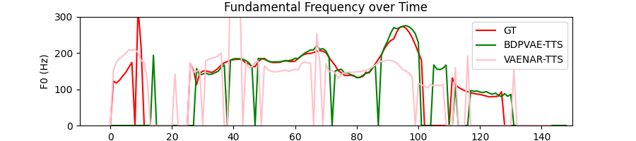
Figure 1: Inference F0 trajectory comparison with VAENAR-TTS of utterance "I suppose I have many thoughts.". The intonation of BDPVAE-TTS is close to the ground truth indicating that our sparse monotonic optimal path approach provides the decoder with a better understanding of how phoneme contributes to the overall acoustic character.

6.1 End-to-end Text-to-Speech

Table 1: Mel Cepstral Distortion (MCD) and Real-Time Factor (RTF) compared with the state-of-the-art TTS models. All models are trained by the same pre-processing setting.

Model	Training	Alignment	MCD	RTF
FastSpeech2 [6] (Baseline)	Non end-to-end	Discrete	9.96 $\pm$ 1.01	3.87 $\times 10^{-4}$
Tacotron2 [25]	End-to-end	Continuous	11.39 $\pm$ 1.95	6.07 $\times 10^{-4}$
VAENAR-TTS [37]	End-to-end	Continuous	8.18 $\pm$ 0.87	1.10 $\times 10^{-4}$
Glow-TTS [1]	End-to-end	Discrete	8.58 $\pm$ 0.89	2.87 $\times 10^{-4}$
BDPVAE-TTS (ours)	End-to-end	Discrete	8.49 $\pm$ 0.96	3.00 $\times 10^{-4}$

We demonstrate applying the BDP-VAE framework with the computational graph of MA to train an end-to-end TTS model on the RyanSpeech [38] dataset. RyanSpeech contains 11279 audio clips (10 hours) of a professional male voice actor’s speech recorded at 44.1kHz. We randomly split 2000 clips for validation and 9297 clips for training. TTS models generate speech according to phoneme tokens in which the duration of phonemes is discrete and unobserved. We redesign the popular TTS model FastSpeech2 [6] into the BDP-VAE framework that is able to capture unobserved hard relationships between phonemes and utterances jointly on both training and inference.

We verify the model performance based on an objective metric, the Mel cepstral distortion (MCD) [39, 40], between the ground truth and the synthesized output. We record inference speed by a real-time factor (RTF) per generated spectrogram frame. We randomly pick 70 sentences from the test set, the numerical results are shown in Table 1. Our method outperforms the baseline [6] on both MCD and RTF and also achieves end-to-end training. Compared to two other end-to-end TTS models [25, 1], the BDPVAE-TTS gets a competitive MCD. Our method gets slightly higher MCD than [37]; however, our BDPVAE-TTS obtains sparse monotonic alignment which provides the decoder a better understanding of how each phoneme contributes to the overall acoustic character. The inference fundamental frequency (F0) shown in Figure 1 shows that the intonation of our method is closer to the ground truth. We provide more F0 comparisons and interpretations in the supplementary material.

6.2 End-to-end Singing Voice Synthesis

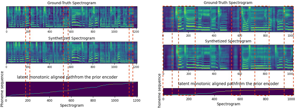
Figure 2: Visualization of the ground truth, synthesized spectrogram, and the monotonically aligned latent optimal path from the conditional prior encoder. Red rectangles indicate that the temporal structure between the generated Mel-spectrogram and the ground truth is almost identical

We extend the BDP-VAE with the computational graph of MA to achieve end-to-end SVS on the popcs dataset [10]. We perform this experiment not to compare with other models as in Section 6.1, but to demonstrate the utility of our method in a related task. In SVS, the longer phoneme duration also provides an opportunity to visualise the monotonically aligned optimal path clearly. The popcs dataset contains 117 Chinese Mandarin pop songs (5 hours) collected from a qualified female vocalist. We randomly split 50 clips for inference and the rest for training. During the inference phase, the conditional inputs are the fundamental frequency and lyrics of the song clips.

Two inference results are visualized in Figure 2 where red rectangles indicate that the temporal structure between the generated Mel-spectrogram and the ground truth is almost identical. This figure shows that, as expected, the latent monotonically aligned path from the prior encoder governs the structure of the phoneme spectrograms generated by the decoder. The latent monotonic optimal path helps the decoder to understand the structure of the unknown spectrogram from phoneme tokens.

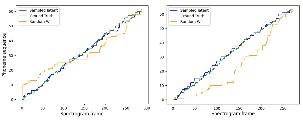
Figure 3: Ground-truth alignment between phonemes and spectrogram frames, a latent optimal path from the encoder, and an optimal path from random $\mathbf{W}$ for two audio clips. BDP-VAE achieves closer alignment with GT, indicating its effectiveness in finding optimal paths in the latent space

6.3 Latent Optimal Path on Computational Graph of DTW

Table 2: Mean absolute error and standard deviation (MAE / MAE $\pm$ STD) for duration on TIMIT.

Model	Latent distribution	Train	Inference
BDP-VAE	$\mathcal{D}(\mathcal{R}_{\text{DTW}},\text{NN}_{\{\phi/\theta\}},1)$	2.92	3.93 $\pm$ 0.37
Baseline	$\mathcal{D}(\mathcal{R}_{\text{DTW}},\mathbf{W}_{\{w\in\mathbf{W}\sim U(0,1)\}},1)$	5.67	5.69 $\pm$ 0.31

To verify the behavior and generalization of the latent optimal paths in BDP-VAE, we obtain latent optimal paths under the computational graph of DTW on the TIMIT speech corpus dataset [41] which includes manually time-aligned phonetic and word transcriptions. TIMIT contains English speech recordings of 630 speakers in eight major dialects of American English. Utterances are recorded as 16-bit 16kHz speech waveform files. We randomly split 50 clips for testing and 580 clips for training.

Following the experimental designs in [18, 42], we set the distribution $\mathcal{D}(\mathcal{R}_{\text{DTW}},\mathbf{W}=\{w\in\mathbf{W}\sim U(0,1)\},1)$ as the baseline due to lack of direct comparison. We take a summation along the spectrogram frame dimension to obtain phoneme duration and compute the mean absolute error (MAE) between the ground truth and the phoneme duration during training. We input phoneme tokens and spectrogram lengths as conditions on inference to obtain latent optimal paths of the prior encoder. We repeat the inference step 5 times and take the average and standard deviation of MAEs as our metric of evaluation. As shown in Table 2, the MAEs of the proposed method are lower than the baseline indicating that the BDP-VAE captures meaningful information to obtain stochastic optimal paths in the latent space and is not merely guessing randomly. Figure 3 visualizes ground-truth alignment, the latent DTW optimal paths from the encoder, and the optimal path from the baseline distribution on two audio clips, which clearly shows the latent optimal path under DTW get a close alignment to the GT. This also indicates the proposed BDP-VAE framework has the ability to capture useful information to obtain sparse DTW optimal paths in its latent space.

6.4 Sensitivity of the Temperature Parameter in BDP-VAE

Table 3: Mean absolute error and standard deviation (MAE / MAE $\pm$ STD) for the duration on TIMIT with different hyper-parameter $\alpha$ settings.

Model	Alpha value	Latent distribution	Train	Inference
BDP-VAE	0.5	$\mathcal{D}(\mathcal{R}_{\text{DTW}},\text{NN}_{\{\phi/\theta\}},0.5)$	2.99	4.40 $\pm$ 0.46
BDP-VAE	1	$\mathcal{D}(\mathcal{R}_{\text{DTW}},\text{NN}_{\{\phi/\theta\}},1)$	2.92	3.93 $\pm$ 0.37
BDP-VAE	1.5	$\mathcal{D}(\mathcal{R}_{\text{DTW}},\text{NN}_{\{\phi/\theta\}},1.5)$	2.94	3.89 $\pm$ 0.35
BDP-VAE	2	$\mathcal{D}(\mathcal{R}_{\text{DTW}},\text{NN}_{\{\phi/\theta\}},2)$	3.01	4.08 $\pm$ 0.27
BDP-VAE	3	$\mathcal{D}(\mathcal{R}_{\text{DTW}},\text{NN}_{\{\phi/\theta\}},3)$	3.25	4.53 $\pm$ 0.10

To study the sensitivity of the temperature parameter $\alpha$, we extend the experiment in Section 6.3. Table 3 shows the MAE value on the training and inference phase with different $\alpha$ settings. The $\alpha$ affects the sharpness of the path distribution: When $\alpha$ is smaller, the sampling is more stochastic. As $\alpha$ increases, the sampling variance decreases. However, when the $\alpha$ value becomes large, the latent optimal path alignment performance decreases, which is consistent with the contribution of temperature in [43]. As $\alpha$ increases, the distribution becomes sharper, while the distribution of paths becomes uniform if the alpha is close to 0. When the distribution tends to be uniform, the optimal alignments sampled are unstable. If the distribution is more categorical, the latent space tends to be a small variation. Since edge weights in the experiments are normalized over the time axis and TIMIT has short audio durations, the model is sensitive to small changes of $\alpha$ value. However, in real applications, the temperature parameter $\alpha$ may depend on edge weights learned by encoders and DAG size which should be carefully chosen.

7 Conclusion

We present a method that captures sparse optimal paths in the latent space relying on the variational autoencoder framework. To this end, we introduce a probabilistic softening solution of the classical optimal path problem on DAGs by using the max and shift properties of the Gumbel distribution. To achieve variational Bayesian inference with latent optimal paths, we give efficient and tractable algorithms for likelihood and KL divergence within the family of path distributions in linear time by dynamic programming, called Bayesian dynamic programming. The BDP-VAE captures sparse optimal paths as latent representations given a DAG and further achieves end-to-end training for generative tasks that rely on unobserved structural relationships. We demonstrated the BDP-VAE with the computational graph of monotonic alignment on two real-world applications to achieve an end-to-end framework (see Figure 1 and Figure 2). We verified the behaviour and generalization of the latent optimal paths under the computational graph of dynamic time warping. We also studied the sensitivity of the hyper-parameter $\alpha$ and gave suggestions for real applications. Our experiments show the success of our approach on generative tasks where it achieves end-to-end training involving unobserved sparse structural optimal paths.
Limitations and Broader Impacts: As a discrete latent variable model, our method uses the REINFORCE estimator which leads to high gradient variance. We will explore more parameterization estimators to reduce the high gradient variance issue of the BDP-VAE in the future. We do not foresee our model bringing negative social impacts.

References

- [1] Jaehyeon Kim, Sungwon Kim, Jungil Kong, and Sungroh Yoon. Glow-tts: A generative flow for text-to-speech via monotonic alignment search. Advances in Neural Information Processing Systems, 33:8067–8077, 2020.
- [2] Buyu Li, Yongchi Zhao, Shi Zhelun, and Lu Sheng. Danceformer: Music conditioned 3d dance generation with parametric motion transformer. In Proceedings of the AAAI Conference on Artificial Intelligence, pages 1272–1279, 2022.
- [3] Xingyu Cai, Tingyang Xu, Jinfeng Yi, Junzhou Huang, and Sanguthevar Rajasekaran. Dtwnet: a dynamic time warping network. Advances in neural information processing systems, 32, 2019.
- [4] Sergio Verdu and H Vincent Poor. Abstract dynamic programming models under commutativity conditions. SIAM Journal on Control and Optimization, 25(4):990–1006, 1987.
- [5] Yi Ren, Yangjun Ruan, Xu Tan, Tao Qin, Sheng Zhao, Zhou Zhao, and Tie-Yan Liu. Fastspeech: Fast, robust and controllable text to speech. Advances in Neural Information Processing Systems, 32, 2019.
- [6] Yi Ren, Chenxu Hu, Xu Tan, Tao Qin, Sheng Zhao, Zhou Zhao, and Tie-Yan Liu. Fastspeech 2: Fast and high-quality end-to-end text to speech. arXiv preprint arXiv:2006.04558, 2020.
- [7] Myeonghun Jeong, Hyeongju Kim, Sung Jun Cheon, Byoung Jin Choi, and Nam Soo Kim. Diff-tts: A denoising diffusion model for text-to-speech. In Hynek Hermansky, Honza Cernocký, Lukás Burget, Lori Lamel, Odette Scharenborg, and Petr Motlícek, editors, Interspeech 2021, 22nd Annual Conference of the International Speech Communication Association, Brno, Czechia, 30 August - 3 September 2021, pages 3605–3609. ISCA, 2021.
- [8] Tavi Halperin, Ariel Ephrat, and Shmuel Peleg. Dynamic temporal alignment of speech to lips. In ICASSP 2019-2019 IEEE International Conference on Acoustics, Speech and Signal Processing (ICASSP), pages 3980–3984. IEEE, 2019.
- [9] Kainan Peng, Wei Ping, Zhao Song, and Kexin Zhao. Non-autoregressive neural text-to-speech. In International conference on machine learning, pages 7586–7598. PMLR, 2020.
- [10] Jinglin Liu, Chengxi Li, Yi Ren, Feiyang Chen, and Zhou Zhao. Diffsinger: Singing voice synthesis via shallow diffusion mechanism. In Proceedings of the AAAI Conference on Artificial Intelligence, pages 11020–11028, 2022.
- [11] Vadim Popov, Ivan Vovk, Vladimir Gogoryan, Tasnima Sadekova, and Mikhail Kudinov. Grad-tts: A diffusion probabilistic model for text-to-speech. In International Conference on Machine Learning, pages 8599–8608. PMLR, 2021.
- [12] Michael McAuliffe, Michaela Socolof, Sarah Mihuc, Michael Wagner, and Morgan Sonderegger. Montreal forced aligner: Trainable text-speech alignment using kaldi. In Francisco Lacerda, editor, Interspeech 2017, 18th Annual Conference of the International Speech Communication Association, Stockholm, Sweden, August 20-24, 2017, pages 498–502. ISCA, 2017.
- [13] Mark Hasegawa-Johnson, Jennifer Cole, Julia Hirschberg, Matthias Jilka, and Richard Tannenbaum. Penn phonetics toolkit (p2tk): A software suite for sound analysis as a function of time. Technical report, Department of Linguistics, University of Pennsylvania, 2005.
- [14] Naihan Li, Shujie Liu, Yanqing Liu, Sheng Zhao, Ming Liu, and Ming Zhou. Close to human quality TTS with transformer. CoRR, abs/1809.08895, 2018.
- [15] Diederik P. Kingma and Max Welling. Auto-encoding variational bayes. In Yoshua Bengio and Yann LeCun, editors, 2nd International Conference on Learning Representations, ICLR 2014, Banff, AB, Canada, April 14-16, 2014, Conference Track Proceedings, 2014.
- [16] Brandon Amos and J. Zico Kolter. Optnet: Differentiable optimization as a layer in neural networks. In Doina Precup and Yee Whye Teh, editors, Proceedings of the 34th International Conference on Machine Learning, ICML 2017, Sydney, NSW, Australia, 6-11 August 2017, volume 70 of Proceedings of Machine Learning Research, pages 136–145. PMLR, 2017.
- [17] Josip Djolonga and Andreas Krause. Differentiable learning of submodular functions. In Isabelle Guyon, Ulrike von Luxburg, Samy Bengio, Hanna M. Wallach, Rob Fergus, S. V. N. Vishwanathan, and Roman Garnett, editors, Advances in Neural Information Processing Systems 30: Annual Conference on Neural Information Processing Systems 2017, December 4-9, 2017, Long Beach, CA, USA, pages 1013–1023, 2017.
- [18] Arthur Mensch and Mathieu Blondel. Differentiable dynamic programming for structured prediction and attention. In International Conference on Machine Learning, pages 3462–3471. PMLR, 2018.
- [19] Gökhan BakIr, Thomas Hofmann, Alexander J Smola, Bernhard Schölkopf, and Ben Taskar. Predicting structured data. MIT press, 2007.
- [20] David Heckerman. A tutorial on learning with bayesian networks. In Michael I. Jordan, editor, Learning in Graphical Models, volume 89 of NATO ASI Series, pages 301–354. Springer Netherlands, 1998.
- [21] Lawrence R. Rabiner. A tutorial on hidden markov models and selected applications in speech recognition. Proc. IEEE, 77(2):257–286, 1989.
- [22] Slav Petrov and Dan Klein. Discriminative log-linear grammars with latent variables. In John C. Platt, Daphne Koller, Yoram Singer, and Sam T. Roweis, editors, Advances in Neural Information Processing Systems 20, Proceedings of the Twenty-First Annual Conference on Neural Information Processing Systems, Vancouver, British Columbia, Canada, December 3-6, 2007, pages 1153–1160. Curran Associates, Inc., 2007.
- [23] Chung-Cheng Chiu and Colin Raffel. Monotonic chunkwise attention. In 6th International Conference on Learning Representations, ICLR 2018, Vancouver, BC, Canada, April 30 - May 3, 2018, Conference Track Proceedings. OpenReview.net, 2018.
- [24] Yuxuan Wang, R. J. Skerry-Ryan, Daisy Stanton, Yonghui Wu, Ron J. Weiss, Navdeep Jaitly, Zongheng Yang, Ying Xiao, Z. Chen, Samy Bengio, Quoc V. Le, Yannis Agiomyrgiannakis, Robert A. J. Clark, and Rif A. Saurous. Tacotron: Towards end-to-end speech synthesis. In Interspeech, 2017.
- [25] Jonathan Shen, Ruoming Pang, Ron J. Weiss, Mike Schuster, Navdeep Jaitly, Zongheng Yang, Zhifeng Chen, Yu Zhang, Yuxuan Wang, RJ-Skerrv Ryan, Rif A. Saurous, Yannis Agiomyrgiannakis, and Yonghui Wu. Natural TTS synthesis by conditioning wavenet on MEL spectrogram predictions. In 2018 IEEE International Conference on Acoustics, Speech and Signal Processing, ICASSP 2018, Calgary, AB, Canada, April 15-20, 2018, pages 4779–4783. IEEE, 2018.
- [26] Yoonhyung Lee, Joongbo Shin, and Kyomin Jung. Bidirectional variational inference for non-autoregressive text-to-speech. In International Conference on Learning Representations, 2021.
- [27] Yuntian Deng, Yoon Kim, Justin T. Chiu, Demi Guo, and Alexander M. Rush. Latent alignment and variational attention. In Samy Bengio, Hanna M. Wallach, Hugo Larochelle, Kristen Grauman, Nicolò Cesa-Bianchi, and Roman Garnett, editors, Advances in Neural Information Processing Systems 31: Annual Conference on Neural Information Processing Systems 2018, NeurIPS 2018, December 3-8, 2018, Montréal, Canada, pages 9735–9747, 2018.
- [28] Lei Yu, Jan Buys, and Phil Blunsom. Online segment to segment neural transduction. arXiv preprint arXiv:1609.08194, 2016.
- [29] Lei Yu, Phil Blunsom, Chris Dyer, Edward Grefenstette, and Tomas Kocisky. The neural noisy channel. arXiv preprint arXiv:1611.02554, 2016.
- [30] Chris J Maddison, Daniel Tarlow, and Tom Minka. A* sampling. Advances in neural information processing systems, 27, 2014.
- [31] Eric Jang, Shixiang Gu, and Ben Poole. Categorical reparameterization with gumbel-softmax. In 5th International Conference on Learning Representations, ICLR 2017, Toulon, France, April 24-26, 2017, Conference Track Proceedings. OpenReview.net, 2017.
- [32] Chris J. Maddison, Andriy Mnih, and Yee Whye Teh. The concrete distribution: A continuous relaxation of discrete random variables. In 5th International Conference on Learning Representations, ICLR 2017, Toulon, France, April 24-26, 2017, Conference Track Proceedings. OpenReview.net, 2017.
- [33] Kirill Struminsky, Artyom Gadetsky, Denis Rakitin, Danil Karpushkin, and Dmitry P. Vetrov. Leveraging recursive gumbel-max trick for approximate inference in combinatorial spaces. In Marc’Aurelio Ranzato, Alina Beygelzimer, Yann N. Dauphin, Percy Liang, and Jennifer Wortman Vaughan, editors, Advances in Neural Information Processing Systems 34: Annual Conference on Neural Information Processing Systems 2021, NeurIPS 2021, December 6-14, 2021, virtual, pages 10999–11011, 2021.
- [34] Xuezhe Ma, Chunting Zhou, Xian Li, Graham Neubig, and Eduard Hovy. FlowSeq: Non-autoregressive conditional sequence generation with generative flow. In Proceedings of the 2019 Conference on Empirical Methods in Natural Language Processing and the 9th International Joint Conference on Natural Language Processing (EMNLP-IJCNLP), pages 4282–4292, Hong Kong, China, November 2019. Association for Computational Linguistics.
- [35] Shakir Mohamed, Mihaela Rosca, Michael Figurnov, and Andriy Mnih. Monte carlo gradient estimation in machine learning. J. Mach. Learn. Res., 21(132):1–62, 2020.
- [36] Hiroaki Sakoe and Seibi Chiba. Dynamic programming algorithm optimization for spoken word recognition. IEEE transactions on acoustics, speech, and signal processing, 26(1):43–49, 1978.
- [37] Hui Lu, Zhiyong Wu, Xixin Wu, Xu Li, Shiyin Kang, Xunying Liu, and Helen Meng. Vaenar-tts: Variational auto-encoder based non-autoregressive text-to-speech synthesis. arXiv preprint arXiv:2107.03298, 2021.
- [38] Rohola Zandie, Mohammad H Mahoor, Julia Madsen, and Eshrat S Emamian. Ryanspeech: A corpus for conversational text-to-speech synthesis. ISCA, 2021.
- [39] Robert Kubichek. Mel-cepstral distance measure for objective speech quality assessment. In Proceedings of IEEE pacific rim conference on communications computers and signal processing, volume 1, pages 125–128. IEEE, 1993.
- [40] Qi Chen, Mingkui Tan, Yuankai Qi, Jiaqiu Zhou, Yuanqing Li, and Qi Wu. V2C: visual voice cloning. In IEEE/CVF Conference on Computer Vision and Pattern Recognition, CVPR 2022, New Orleans, LA, USA, June 18-24, 2022, pages 21210–21219. IEEE, 2022.
- [41] J. Garofolo, Lori Lamel, W. Fisher, Jonathan Fiscus, D. Pallett, N. Dahlgren, and V. Zue. Timit acoustic-phonetic continuous speech corpus. Linguistic Data Consortium, 11 1992.
- [42] Aaron Van Den Oord, Oriol Vinyals, et al. Neural discrete representation learning. Advances in neural information processing systems, 30, 2017.
- [43] J. Platt. Probabilistic outputs for support vector machines and comparison to regularized likelihood methods. In Advances in Large Margin Classifiers, 2000.