Meterwavelength Single-pulse Polarimetric Emission Survey. VI. Towards understanding the Phenomenon of Pulsar Polarization in Partially Screened Vacuum Gap model.

Abstract

We have observed 123 pulsars with periods longer than 0.1 seconds in the Meterwavelength Single-pulse Polarimetric Emission Survey. In this work a detailed study of polarization behaviour of these pulsars have been carried out. We were able to fit the rotating vector model to the polarization position angle sweeps in 68 pulsars, and in 34 pulsars the emission heights could be measured. In all cases the radio emission was constrained to arise below 10% of the light cylinder radius. In pulsars with low spindown energy loss, $\dot{E}<10^{34}$ ergs s^-1, we found the mean fractional linear polarization of the individual times samples in single pulses to be around 0.57 (57%) which is significantly larger than the fractional linear polarization of 0.29 (29%) obtained from the average profiles. On the other hand the mean fractional circular polarization of the individual time samples in single pulses is around 0.08 (8%), similar to the measurements from the average profiles. To explain the observed polarization features, we invoke the partially screened vacuum gap model of pulsars, where dense spark associated plasma clouds exist with high pair plasma multiplicity, with significant decrease of density in the regions between the clouds, that are dominated by iron ions. The coherent radio emission is excited by curvature radiation from charge bunches in these dense plasma clouds and escape as linearly polarized waves near cloud boundaries. We suggest that the circular polarization arises due to propagation of waves in the low pair multiplicity, ion dominated inter-cloud regions.

1 Introduction

The pulsar magnetosphere is composed of dense electron-positron pair plasma embedded in strong magnetic fields, and can be divided into regions of open and closed magnetic field lines (Goldreich & Julian 1969). A mix of relativistically charged particles, comprising of pair plasma as well as beams of positrons and iron ions, stream outward along the open magnetic field lines (Ruderman & Sutherland 1975; Cheng & Ruderman 1977). The coherent radio emission in pulsars arises due to growth of plasma instabilities in the relativistically streaming plasma (see e.g. Ginzburg & Zhelezniakov, 1975). In most cases the radio emission from pulsars is seen to exhibit high levels of linear polarization as well as significant circular polarization (e.g. Manchester et al. 1975; Gould & Lyne 1998). The nature of polarization is determined by the processes by which the radio emission is generated and the subsequent propagation effects in the pulsar magnetosphere. A major theoretical challenge is to understand these physical mechanisms that give rise to the observed polarization features (see e.g. Melrose, 1995, for a review).

Radio polarization behaviour of pulsars can be quantified using two different schemes of measurements : the average profiles (hereafter AP), where the Stokes parameters are obtained by averaging a large number of pulses; and single pulses (hereafter SP) where the Stokes parameters are obtained collating from individual bright pulses. The AP studies are sufficient for understanding several aspects of polarization behaviour in normal pulsars ($P>$ 50 msec). The most prominent behaviour is the polarization position angle (PPA) of the linear polarization showing a characteristic S-shaped traverse across the pulse window and can be interpreted in terms of the rotating vector model (RVM) which was first proposed by Radhakrishnan & Cooke (1969). According to the RVM the swing of the PPA arises when the observer’s line of sight (LOS) cuts across the dipolar magnetic field line plane and is determined by the LOS geometry, characterised by the angle between the rotation axis and magnetic axis, $\alpha$, and the angle between the rotation axis and the LOS during closest approach, $\beta$. Thus finding suitable RVM fits to the observed the PPA traverse in principle should constrain the LOS geometry of the pulsar (Everett & Weisberg, 2001; von Hoensbroech & Xilouris, 1997a). However, in all practical purposes only the shape of the PPA traverse and it’s steepest gradient point (hereafter SGP) can be used to the extent of distinguishing between central and tangential cuts across the pulsar emission beams and not the detailed geometry, since the angles $\alpha$ and $\beta$ obtained from the RVM fits are found to be highly correlated.

AP measurement of linear polarization PPAs in conjunction with total intensity profiles can also be used to determine the radio emission heights, utilizing the relative shifts that arise between them due to aberration-retardation effects (hereafter A/R, Blaskiewicz et al., 1991). The A/R method puts tight constraints on the emission height to be below 10% of the light cylinder distance. The A/R effect have been studied recently for a large sample of pulsars around 1 GHz (Johnston et al. 2023), although for lower and higher than 1 GHz frequency bands relatively small sample of pulsars have been studied (see Mitra (2017) and references therein). APs have also been used to estimate the nature of emission beam shape at radio frequencies. In most works the beam is considered to have a core-cone structure, with a central core and nested conal components, and follows a distinct radius to frequency mapping where lower frequencies are found to arise at progressively higher heights from the neutron star surface (see e.g. Rankin, 1983, 1993; Mitra & Deshpande, 1999; Mitra & Rankin, 2002). Using relatively fewer pulsars Morris et al. (1981) showed that depolarization of AP is higher for older, longer period pulsars compared to shorter period, younger pulsars. Subsequent works on larger samples have found that the degree of linear polarization ($\%L$) correlates with the spindown energy loss ($\dot{E}$), with low $\dot{E}$ pulsars having $\%L$ of about 20% and high $\dot{E}$ pulsars about 80% (Weltevrede & Johnston, 2008; Johnston & Kerr, 2018; Mitra et al., 2016; Olszanski et al., 2019; Posselt et al., 2022). A change in the beam shape properties between high and low $\dot{E}$ pulsars has also been suggested by Karastergiou & Johnston (2007).

The SP studies on the other hand reveal dynamic emission features like mode changing, subpulse drifting, nulling, microstructures, periodic amplitude modulation, etc., (Rankin, 1986; Weltevrede et al., 2006; Mitra et al., 2015; Basu et al., 2016, 2020a; Song et al., 2023). Mode changing, nulling and subpulse drifting are usually associated with low energetic pulsars, while periodic amplitude modulations are seen in more energetic systems (Basu et al., 2020a). For example, the SP phenomenon of subpulse drifting shows a prominent dependence on the spindown energy loss and is only seen in pulsars with $\dot{E}<5\times 10^{32}$ ergs s^-1 (Basu et al., 2016, 2019). The PPA distribution obtained from SP in low $\dot{E}$ pulsars often show the presence of orthogonal polarization modes (OPM) where two orthogonal RVM tracks, separated by 90$\arcdeg$ in phase, can be identified. In some cases they are highly disordered and do not resemble a S-shaped curve corresponding to RVM. The high $\dot{E}$ pulsars on the hand generally have a single PPA track that can mostly be identified with the RVM (Mitra et al., 2016).

The preceding discussion highlights that a distinct trend has emerged from recent works, involving both AP and SP measurements, suggesting a change in radio emission properties as a function of $\dot{E}$. At the higher $\dot{E}$ range certain pulsar radio emission properties appear to be quite different from the lower energetic population. In this work we further explore whether the SP fractional linear polarization changes with $\dot{E}$ in a manner similar to their behaviour in APs. Either the depolarization of APs in low $\dot{E}$ pulsars arises due to all SPs having intrinsically low fractional linear polarization; or it is possible that the individual SPs have high fractional linear polarization that reduces during the averaging process. Understanding such trends in the general pulsar population requires observations of a large number of pulsars with high sensitivity detection of polarized SPs.

A large number of studies exist in the literature that have been devoted towards understanding the polarization properties in pulsars. The radio emission is generated in the inner magnetosphere where a dense pair plasma is present in very high magnetic fields. In such systems it can be shown that there exist two distinct plasma modes that are linearly polarized, the extraordinary (X) mode, with the electric vector being perpendicular to the propagation vector and the local magnetic field, and ordinary (O) mode, with the electric vector lying in the plane of the propagation vector and the local magnetic field, respectively (see Volokitin et al., 1985; Lominadze et al., 1986; Arons & Barnard, 1986). Generally, the observed OPMs in pulsars are associated with the naturally occurring orthogonal wave modes that are excited by a suitable emission mechanism arising in the pair plasma. The two modes split in the plasma during propagation due to their different refractive indices, and travel with different phase velocities, and eventually emerge as OPMs (Melrose, 1979; Melikidze et al., 2014). The circular polarization arises either due to an intrinsic emission process or as a result of propagation effects (Allen & Melrose, 1982; Kazbegi et al., 1991; Wang et al., 2010). Observations show that individual OPMs are elliptically polarized, even when very high level of linear polarization is seen in SPs, and strongly favour the propagation effects being the underlying cause. However, the theoretical premise where both the emission mechanism and the propagation effect is addressed in a self consistent manner is still missing.

The Meterwavelength single-pulse polarimetric emission survey (MSPES) was conducted using the Giant Meterwave Radio Telescope (GMRT) primarily to increase the available sample for AP/SP studies (hereafter PaperI, Mitra et al., 2016). The GMRT consists of a Y-shaped array of 30 antennas of 45 m diameter, with 14 antennas located within a central one square kilometer area and the remaining 16 antennas placed along the three arms, which have a maximum distance of 27 km (Swarup et al. 1991). The MSPES observations were carried out at two different frequencies centered around 325 and 610 MHz with a bandwidth of 16.67 MHz at each frequency (see PaperI for details). These observations contributed towards detailed characterisation of the subpulse drifting behaviour in pulsars (Basu et al., 2016, 2019), and were instrumental in demonstrating that subpulse drifting arises from a partially screened vacuum gap (PSG, Gil et al., 2003; Basu et al., 2020b, 2022a, 2023). The highly polarized single pulses (Mitra et al., 2009, 2023) and variation in pulsar spectral nature across the emission beam (Basu et al., 2021, 2022b) have provided compelling evidence that the coherent radio emission is excited by curvature radiation from charge bunches. In this paper we use the MSPES observations to measure the radio emission heights in pulsars using APs, and further compare the SP polarization properties with AP. In section 2, the RVM fits to the PPA in all relevant cases have been shown and the radio emission heights have been found using A/R shifts. In section 3 we have shown the variation of the SP polarization properties with $\dot{E}$. In Section 4 we use the PSG model and coherent curvature radiation mechanism to understand the origin of linear and circular polarization properties of normal pulsars, followed by the conclusion presented in section 5.

2 RVM fits and Emission heights using A/R method

Figure 1: The typical AP and SP polarization properties of three pulsars with different $\dot{E}$ values are shown. Left column represents the highly polarized PSR J0742-2822 with $\dot{E}=1.43\times 10^{35}$ ergs s^-1, middle column corresponds to PSR J1752-2806 with $\dot{E}=1.8\times 10^{33}$ ergs s^-1 and the right column shows the polarization behaviour of PSR J0034-0721 with $\dot{E}=1.92\times 10^{31}$ ergs s^-1. Top panels (upper window) show the average profile with total intensity (Stokes I; solid black lines), total linear polarization (dashed red line) and circular polarization (Stokes V; dotted blue line). Top panels (lower window) also show the single pulse PPA distribution (colour scale) along with the average PPA (red error bars). The RVM fits to the average PPA (dashed pink line) in case of PSR J0742-2822 and PSR J0034-0721 is also shown in this plot. No suitable RVM fit was possible for the disordered PPA distribution of PSR J1752-2806. Middle panels show the $\chi^{2}$ contours for the parameters $\alpha$ and $\beta$ obtained from RVM fits. Bottom panels show the Hammer-Aitoff projection of the polarized time samples with the colour scheme representing the fractional polarization level. (The complete set of figures (88 figures) are available in the appendix  E).

The RVM gives an estimate of the PPA, $\Psi$, as a function of the pulse longitude, $\phi$, in terms of the geometrical angles $\alpha$ and $\beta$ as :

$$\Psi=\Psi_{\circ}+\\ \tan^{-1}{\left(\frac{\sin{\alpha}\sin{(\phi-\phi_{\circ})}}{\sin{(\alpha+\beta)}\cos{\alpha}-\sin{\alpha}\cos{(\alpha+\beta)}\cos{(\phi-\phi_{\circ})}}\right)}\\$$ (1)

Here, $\Psi_{\circ}$ and $\phi_{\circ}$ are the phase offsets of $\Psi$ and $\phi$ respectively. At the longitude $\phi_{\circ}$, where the PPA is $\Psi_{\circ}$, the rotation axis and the magnetic axis lie in the same plane and the PPA traverse goes through an inflexion point. The steepest gradient of the PPA traverse also corresponds to this inflexion point, and has a dependence $\mid d\Psi/d\phi\mid_{max}=\sin{\alpha}/\sin{\beta}$. We have carried out suitable fits to the PPA, using Eq. 1, in all pulsars of the MSPES sample that exhibits smoothly varying monotonic RVM like behaviour, by minimizing $\chi^{2}$. Examples of RVM fits to the PPA are shown in Fig. 1 (see pink dashed line in lower window of top panels). The estimated values of the angles $\alpha$ and $\beta$ from the RVM fits are highly correlated and cannot be used to constrain the pulsar LOS geometry (von Hoensbroech & Xilouris, 1997b; Everett & Weisberg, 2001; Mitra & Li, 2004). This is also evident from the $\chi^{2}$ variations as a function of $\alpha$ and $\beta$ in Fig. 1 (see middle panels). The above analysis also allows for the determination of $\Psi_{\circ}$ and $\phi_{\circ}$, as indicated in Fig. 1 (see black error bar in lower window of top panels).

Despite their inadequacy in constraining the LOS geometry, the RVM fits to the PPA can yield robust estimates of radio emission heights by taking into account the shifts due to the A/R effect. If the radio emission region arises close to the stellar surface, less than 10% of the light cylinder distance, then due to pulsar rotation, the aberration and retardation causes a positive shift, $\Delta\phi$, of the phase of the steepest gradient point, $\psi_{\circ}$, from the center of the profile. Blaskiewicz et al. (1991) showed that if the emission across the pulse profile arises at a height $h$, it can be related to this shift as :

$$h=\cfrac{cP\Delta\phi}{1440}~{}~{}~{}\mathrm{km},$$ (2)

here $c$ is the velocity of light and $P$ the rotation period of the pulsar. It was further shown by Pétri & Mitra (2020) that these estimates using A/R shifts remain valid up to heights less than 20% of the light cylinder radius, even when deviations from a star centered static dipole structure, due to perturbations introduced by rotating plasma, are taken into account. A number of studies in the literature have used the A/R method to find estimates of the emission height in the normal pulsar population, and showed the radio emission to arise below 10% of the light cylinder radius (Blaskiewicz et al., 1991; von Hoensbroech & Xilouris, 1997a; Mitra & Li, 2004; Weltevrede & Johnston, 2008; Mitra & Rankin, 2011).

The estimation of $h$ using Eq. 2 has certain underlying assumptions regarding the relevant quantities that require careful considerations. $\Delta\phi$ is obtained from the difference between $\phi_{\circ}$ and the center of the total intensity profile, $\phi_{c}$. RVM fits to the PPA yields $\phi_{\circ}$, while $\phi_{c}$ is obtained by identifying the phases corresponding to the leading and trailing edges of the profile, $\phi_{l}$ and $\phi_{t}$, respectively, such that $\phi_{c}=\phi_{l}+(\phi_{t}-\phi_{l})/2$, and $\Delta\phi=\phi_{\circ}-\phi_{c}$. The first assumption for the above scheme to be applicable is for the emission height to be constant across the entire pulse profile. This can be considered reasonable if the estimated RVM clearly fits the observed PPA traverse, providing a robust estimate for $\phi_{\circ}$. On the other hand, if the emission height shows large variations across the profile, the PPA traverse will show differential height dependent A/R effect and deviate from the RVM nature (Mitra & Seiradakis, 2004). The second assumption is connected with the estimates of $\phi_{l}$ and $\phi_{t}$, which are expected to be associated with the last open magnetic field lines on either side of the LOS cut across the emission beam. In practical purposes $\phi_{l}$ and $\phi_{t}$ are identified from the profile edges lying above the detection threshold, as specified by the background noise levels. If the profiles are detected with high signal to noise levels, the above assumption is more reasonable, although the pulsar emission can become significantly weaker at the profile edges and may still lead to inaccuracies. In more severe cases the estimated $\Delta\phi$ has negative values which is incompatible with the A/R predictions. In most reported works the estimated $h$ from positive $\Delta\phi$ were around a few hundred kilometers, with the measured $\Delta\phi$ values varying by an order of magnitude between faster and slower pulsars, as expected from Eq. 2, thereby highlighting the efficacy of the A/R method. In this context a negative estimate for $\Delta{\phi}$ can certainly be attributed to the improper identification of the last open magnetic field line in the pulsar profile.

We have used the A/R method to estimate the emission heights of the pulsars observed in MSPES. We identified $\phi_{l}$ and $\phi_{t}$ from the profile edges at 5 times the noise level, while $\phi_{\circ}$ was obtained from the RVM fits to the PPA, see Table 1. The errors in estimating $\phi_{t}$ and $\phi_{l}$ were calculated using the prescription of Kijak & Gil (1997, see equation 4). The error in $\phi_{\circ}$ was obtained by computing the variation of $\phi_{\circ}$ from various combinations of $\alpha$ and $\beta$ lying within two times the minimum $\chi^{2}$ value obtained from the fit. This leads to asymmetric errors in $\phi_{\circ}$ (see Fig. 1), however in Table 1 only the average value is reported, which is further used for the error estimate of $\Delta{\phi}$ and $h$.

Table 1: The measurements of 68 pulsars from the MSPES sample where it was possible to obtain suitable RVM fits to the PPA traverse. Column 2 to 4 reports the observing frequency in MHz, Jname and period in seconds. Column 5 presents the minimum $\chi^{2}$ of the fits, Column 6 to 8 presents the phase of the trailing edge, $\phi_{t}$, the leading edge, $\phi_{l}$, of the pulsar profile and the phase of the steepest gradiant point, $\phi_{\circ}$. Column 9 reports the the shift between midpoint of the profile and the SG point, $\Delta\phi$, while Column 10 shows our estimate of the emission height, $h$, using Eq. 2. Note that generally errors in $\phi_{\circ}$ are asymmetric, however here only the average value is quoted, which is further used to find the error in $\Delta\phi$ and $h$.

	Freq	PSR	Period	$\chi^{2}$	$\phi_{l}$	$\phi_{t}$	$\phi_{\circ}$	$\Delta\phi$	$h$
	(MHz)		(sec)		(∘)	(∘)	(∘)	(∘)	(km)
1	333	J0034-0721	0.943	2.5	-23.5$\pm$0.1	26.2$\pm$0.1	9.8$\pm$50	—	—
2	618	J0151-0635	0.833	1.3	-6.6$\pm$0.1	31.2$\pm$0.1	12$\pm$2	-0.3$\pm$2	—
3	333	J0304+1932	1.387	1.3	-16.5$\pm$0.1	4.9$\pm$0.1	-5.3$\pm$0.1	0.5$\pm$0.1	144$\pm$29
	618	J0304+1932	1.387	1.3	-14.4$\pm$0.1	5.1$\pm$0.1	-3.8$\pm$0.1	0.8$\pm$0.1	230$\pm$29
4	333	J0452-1759	0.549	3.2	-17.6$\pm$0.1	17.3$\pm$0.1	3.8$\pm$1.0	3.9$\pm$1	457$\pm$114
	618	J0452-1759	0.549	1.2	-14.6$\pm$0.2	14.3$\pm$0.2	3.2$\pm$2.0	4.0$\pm$2	457$\pm$228
5	333	J0525+1115	0.354	23.5	-3.2$\pm$0.2	19.7$\pm$0.2	10.2$\pm$2.0	3.0$\pm$2	221$\pm$147
	618	J0525+1115	0.354	1.9	-13.2$\pm$0.3	3.5$\pm$0.3	-1.2$\pm$3.0	3.6$\pm$3	265$\pm$221
6	333	J0528+2200	3.746	1.5	-5.0$\pm$0.1	19.9$\pm$0.1	7.6$\pm$0.5	0.2$\pm$0.5	—
7	333	J0543+2329	0.246	1.2	-12.0$\pm$0.3	27.2$\pm$0.3	27.9$\pm$8.0	20$\pm$8	1025$\pm$410
	618	J0543+2329	0.246	0.9	-11.2$\pm$0.3	24.8$\pm$0.3	24.6$\pm$6	17.8$\pm$6	912$\pm$307
8	333	J0614+2229	0.335	1.02	-8.1$\pm$0.3	11.5$\pm$0.3	3.2$\pm$15	1.5$\pm$15	—
	618	J0614+2229	0.335	0.8	-5.2$\pm$0.3	5.9$\pm$0.3	9.5$\pm$10	9.1$\pm$10	—
9	333	J0629+2415	0.477	10.5	-7.8$\pm$0.2	16.2$\pm$0.2	-0.1$\pm$1	-4.0$\pm$1	—
	618	J0629+2415	0.477	13.6	-7.8$\pm$0.2	11.9$\pm$0.2	1.0$\pm$2	-1.0$\pm$2	—
10	333	J0630-2834	1.245	1.7	-35.8$\pm$0.1	38.1$\pm$0.1	2.7$\pm$1	1.6$\pm$1	415$\pm$259
	618	J0630-2834	1.245	1.5	-23.6$\pm$0.1	29.9$\pm$0.1	2.7$\pm$1	-1.0$\pm$1	—
11	333	J0659+1414	0.384	0.9	-16.1$\pm$0.2	14.9$\pm$0.2	19.4$\pm$15	20$\pm$15	1600$\pm$1200
	618	J0659+1414	0.384	1.6	-13.7$\pm$0.2	13.6$\pm$0.2	15.6$\pm$30	—	—
12	333	J0729-1836	0.510	0.9	-5.8$\pm$0.2	18.9$\pm$0.2	8.6$\pm$2	2$\pm$2	—
	618	J0729-1836	0.510	1.0	-3.9$\pm$0.2	15.7$\pm$0.2	8.0$\pm$3	2$\pm$3	—
13	618	J0742-2822	0.167	9.1	-10.6$\pm$0.5	16.9$\pm$0.5	9.1$\pm$1	3$\pm$1	104$\pm$35
14	333	J0846-3533	1.116	1.0	-22.2$\pm$0.1	10.1$\pm$0.1	-6.8$\pm$1	-0.7$\pm$2	—
	618	J0846-3533	1.116	2.4	-19.5$\pm$0.1	6.8$\pm$0.1	-5.6$\pm$1	0.7$\pm$2	—
15	618	J0905-4536	0.988	1.8	-6.6$\pm$0.1	53.8$\pm$0.1	24.9$\pm$8	1.3$\pm$8	—
16	618	J0922+0638	0.431	8.8	-14.2$\pm$0.2	6.6$\pm$0.2	3.4$\pm$1	7.2$\pm$1	646$\pm$90
17	333	J0944-1354	0.570	74.0	-2.8$\pm$0.2	5.7$\pm$0.2	1.4$\pm$0.5	0.0$\pm$0.5	—
	618	J0944-1354	0.570	6.3	-3.1$\pm$0.2	4.0$\pm$0.2	0.8$\pm$0.1	0.2$\pm$0.2	—
18	333	J0953+0755	0.253	20.6	-172$\pm$0.4	84.4$\pm$0.4	-11$\pm$8	33$\pm$8	1793$\pm$421
	618	J0953+0755	0.253	22.6	-171$\pm$0.4	66.3$\pm$0.4	-4$\pm$4	48$\pm$4	2530 $\pm$210
19	618	J0959-4809	0.670	1.6	-54$\pm$0.2	9.1 $\pm$0.2	-23$\pm$3	-0.5$\pm$3	—
20	618	J1034-3224	1.151	2.3	-39$\pm$0.1	50.1$\pm$0.1	11.4$\pm$9	5.9$\pm$9	—
21	618	J1041-1942	1.386	1.6	-2.3$\pm$0.1	15.7 $\pm$0.1	7.3$\pm$0.3	0.6$\pm$0.3	173 $\pm$ 86
22	333	J1136+1551	1.188	84	-7.3$\pm$0.1	12.1 $\pm$0.1	4.2$\pm$0.5	1.8$\pm$0.5	445 $\pm$ 124
	618	J1136+1551	1.188	25	-3.2$\pm$0.1	9.6 $\pm$0.1	3.1$\pm$2.5	0$\pm$2.5	—
23	333	J1239+2453	1.382	9.4	-3.2$\pm$0.1	15.1 $\pm$0.1	6.7$\pm$0.5	0.75$\pm$0.5	215 $\pm$ 143
	618	J1239+2453	1.382	12.4	-2.3$\pm$0.1	13.3 $\pm$0.1	5.7$\pm$0.5	0.2$\pm$0.5	—
24	618	J1321+8323	0.670	3.2	-4.5$\pm$0.1	12.8 $\pm$0.1	7.7$\pm$9	2$\pm$9	—
25	333	J1328-4357	0.533	1.4	-3.0$\pm$0.2	12.0 $\pm$0.2	4.1$\pm$1	-0.4$\pm$1	—
	618	J1328-4357	0.533	13.1	-6.7$\pm$0.2	6.4 $\pm$0.2	-1.1$\pm$1	-0.9$\pm$1	—
26	333	J1328-4921	1.479	10.5	-15.1$\pm$0.1	2.7 $\pm$0.1	-6.5$\pm$1	-0.3$\pm$1	—
	618	J1328-4921	1.479	1.5	-13.5$\pm$0.1	2.3 $\pm$0.1	-6.1$\pm$1	-0.5$\pm$1	—
27	333	J1507-4352	0.287	1.1	-7.1 $\pm$0.3	4.9 $\pm$0.3	1.9$\pm$1	3$\pm$1	179 $\pm$60
	618	J1507-4352	0.287	0.8	-5.6 $\pm$0.3	4.9 $\pm$0.3	2.0$\pm$1	2.3$\pm$1	138 $\pm$60
28	333	J1527-3931	2.418	6.1	-2.1 $\pm$0.1	5.7 $\pm$0.1	1.7$\pm$0.5	-0.1$\pm$0.5	—
	618	J1527-3931	2.418	1.6	-1.5 $\pm$0.1	4.7 $\pm$0.1	1.5$\pm$0.5	-0.1$\pm$0.5	—
29	333	J1555-3134	0.518	1.2	-20.4 $\pm$0.2	6.4 $\pm$0.2	-7.4$\pm$5	-0.7$\pm$5	—
	618	J1555-3134	0.518	2.3	-4.4 $\pm$0.2	19.2 $\pm$0.2	13.1$\pm$10	5.7$\pm$10	—
30	333	J1559-4438	0.257	3.1	-25.3 $\pm$0.3	16.4 $\pm$0.3	-6.5$\pm$1	-2.1$\pm$1	—
	618	J1559-4438	0.257	11.1	-28.1 $\pm$0.3	15.7 $\pm$0.3	-5.3$\pm$1	1.0$\pm$1	—
31	333	J1603-2531	0.283	0.9	-4.8 $\pm$0.3	5.8 $\pm$0.3	8.3$\pm$20	$\pm$	—
	618	J1603-2531	0.283	1.3	-7.3 $\pm$0.3	7.0 $\pm$0.3	13.7$\pm$55	$\pm$	—
32	618	J1700-3312	1.358	1.0	-1.9 $\pm$0.1	11.5 $\pm$0.1	5.5$\pm$0.5	0.7$\pm$0.5	198 $\pm$ 141
33	333	J1703-3241	1.212	5.2	-10.1 $\pm$0.1	10.6 $\pm$0.1	-0.5$\pm$0.5	-0.75$\pm$0.5	—
	618	J1703-3241	1.212	7.8	-4.6 $\pm$0.1	12.3 $\pm$0.1	4.0$\pm$0.5	0.15$\pm$0.5	—
34	333	J1709-1640	0.653	2.3	-11.7 $\pm$0.1	6.6 $\pm$0.1	-1.7$\pm$0.5	0.8$\pm$0.5	108 $\pm$68
	618	J1709-1640	0.653	1.8	-10.2 $\pm$0.1	5.9 $\pm$0.1	-0.3$\pm$0.5	1.9$\pm$0.5	258 $\pm$68
35	618	J1709-4429	0.103	1.2	-28.0 $\pm$0.8	22.0 $\pm$0.8	5.2$\pm$15	8$\pm$15	—
36	333	J1720-2933	0.620	1.3	-9.7 $\pm$0.1	15.8 $\pm$0.1	2.8$\pm$2	-0.3$\pm$2	—
	618	J1720-2933	0.620	1.3	-15.1 $\pm$0.1	7.7 $\pm$0.1	-3.2$\pm$2	0.5$\pm$2	—
37	333	J1722-3712	0.236	1.5	-9.4 $\pm$0.4	14.6 $\pm$0.4	-7.2$\pm$10	-9.8$\pm$10	—
	618	J1722-3712	0.236	0.7	-10.1 $\pm$0.4	6.4 $\pm$0.4	4.7$\pm$6	6.5$\pm$6	—
38	618	J1733-3716	0.338	1.4	-5.6 $\pm$0.3	48.9 $\pm$0.3	29.2$\pm$8	7.5$\pm$8	—
39	333	J1740+1311	0.803	7.0	-15.9 $\pm$0.1	11.3 $\pm$0.1	-1.0$\pm$0.5	1.3$\pm$0.5	217$\pm$ 83
	618	J1740+1311	0.803	20.5	-6.3 $\pm$0.1	19.8 $\pm$0.1	8.7$\pm$0.5	1.9$\pm$0.5	317 $\pm$ 83
40	333	J1741-0840	2.043	1.2	-17.1 $\pm$0.1	3.3 $\pm$0.1	-6.4$\pm$0.5	0.5$\pm$0.5	—
	618	J1741-0840	2.043	1.1	-15.2 $\pm$0.1	2.6 $\pm$0.1	-5.9$\pm$0.5	0.4$\pm$0.5	—
41	618	J1741-3927	0.512	2.7	-9.1 $\pm$0.1	12.2 $\pm$0.1	4.4$\pm$3.2	2.8$\pm$3.2	—
42	333	J1751-4657	0.742	92.5	-5.1 $\pm$0.1	9.3 $\pm$0.1	2.4$\pm$0.5	0.3$\pm$0.5	—
	618	J1751-4657	0.742	23.5	-3.8 $\pm$0.1	8.5 $\pm$0.1	1.6$\pm$0.5	-0.7$\pm$0.5	—
43	333	J1801-0357	0.921	8.7	-7.0 $\pm$0.1	5.9 $\pm$0.1	-0.6$\pm$0.5	0.0$\pm$0.5	—
	618	J1801-0357	0.921	4.1	-7.0 $\pm$0.1	3.6 $\pm$0.1	-1.7$\pm$1.0	0.0$\pm$0.5	—
44	333	J1801-2920	1.082	3.6	-11.9 $\pm$0.1	11.6 $\pm$0.1	0.2$\pm$0.5	0.4$\pm$0.5	—
	618	J1801-2920	1.082	5.4	-2.1 $\pm$0.1	18.1 $\pm$0.1	8.5$\pm$0.5	0.5$\pm$0.5	—
45	333	J1807-0847	0.164	1.6	-18.3 $\pm$0.5	31.4 $\pm$0.5	-11.9$\pm$12	-18$\pm$12	—
	618	J1807-0847	0.164	13.7	-16.7 $\pm$0.5	15.1 $\pm$0.5	-6.9$\pm$8	-6$\pm$8	—
46	333	J1808-0813	0.876	1.8	-10.4 $\pm$0.1	10.9 $\pm$0.1	-9.9$\pm$5	-6.2$\pm$5	—
	618	J1808-0813	0.876	0.9	-11.1 $\pm$0.1	4.1 $\pm$0.1	0.3$\pm$1	3.8$\pm$1	693 $\pm$ 182
47	333	J1816-2650	0.593	1.3	-30.6 $\pm$0.1	9.3 $\pm$0.1	-8.5$\pm$6	2.1$\pm$6	—
	618	J1816-2650	0.593	1.3	-3.2 $\pm$0.1	26.4 $\pm$0.1	15.8$\pm$7	4.2$\pm$7	—
48	618	J1820-0427	0.598	79.3	-7.6 $\pm$0.2	8.8 $\pm$0.2	-0.1$\pm$1	-0.7$\pm$1	—
49	333	J1822-2256	1.874	1.4	-15.9 $\pm$0.1	10.1 $\pm$0.1	-6.9$\pm$5	-4$\pm$5	—
	618	J1822-2256	1.874	1.1	-11.1 $\pm$0.1	4.9 $\pm$0.1	-4.2$\pm$8	-1$\pm$8	—
50	333	J1823-3106	0.284	5.2	-12.3 $\pm$0.3	10.1 $\pm$0.3	3.0$\pm$2	4.1$\pm$2	242 $\pm$ 118
	618	J1823-3106	0.284	0.9	-8.6 $\pm$0.3	6.4 $\pm$0.3	1.7$\pm$2	2.8$\pm$2	165 $\pm$ 118
51	333	J1834-0426	0.290	4.7	-56.1 $\pm$0.3	69.3 $\pm$0.3	16.4$\pm$10	9.8$\pm$10	—
	618	J1834-0426	0.290	4.0	-21.9 $\pm$0.3	103.7 $\pm$0.3	58.5$\pm$6	17.6$\pm$6	1063 $\pm$ 362
52	618	J1835-1106	0.166	0.6	-9.3 $\pm$0.5	10.4 $\pm$0.5	-1.7$\pm$12	-2.25$\pm$12	—
53	333	J1841+0912	0.381	1.5	-7.3 $\pm$0.2	4.5 $\pm$0.2	0.7$\pm$0.5	2.1$\pm$0.5	167 $\pm$ 40
	618	J1841+0912	0.381	1.2	-7.8 $\pm$0.2	5.9 $\pm$0.2	-0.6$\pm$0.3	0.7$\pm$0.3	47 $\pm$ 23
54	618	J1842-0359	1.840	1.2	-62.2 $\pm$0.1	10.6 $\pm$0.1	-26.1$\pm$1	-0.3$\pm$0.5	—
55	333	J1900-2600	0.612	95	-26.3 $\pm$0.1	21.9 $\pm$0.1	-3.9$\pm$2	-1.7$\pm$2	—
	618	J1900-2600	0.612	22	-38.0 $\pm$0.1	5.3 $\pm$0.1	-19.2$\pm$2	-2.8$\pm$2	—
56	333	J1901-0906	1.782	1.8	-12.4 $\pm$0.1	2.5 $\pm$0.1	-5.1$\pm$4	-0.2$\pm$4	—
	618	J1901-0906	1.782	14.1	-10.2 $\pm$0.1	1.7 $\pm$0.1	-2.9$\pm$6	1.3$\pm$6	—
57	333	J1910+0358	2.330	1.9	-65.6 $\pm$0.1	6.1 $\pm$0.1	-31.3$\pm$1	-1.5$\pm$1	—
	618	J1910+0358	2.330	1.8	-59.4 $\pm$0.1	6.2 $\pm$0.1	-27.8$\pm$1	-1.1$\pm$1	—
58	333	J1917+1353	0.195	1.9	-11.6 $\pm$0.5	13.4 $\pm$0.5	7.6$\pm$2	6.7$\pm$2	272 $\pm$ 81
	618	J1917+1353	0.195	1.5	-8.4 $\pm$0.5	10.7 $\pm$0.5	8.2$\pm$4	7.0$\pm$4	333 $\pm$ 162
59	618	J1919+0134	1.604	1.5	-14.6 $\pm$0.1	2.8 $\pm$0.1	-5.3$\pm$9	0.6$\pm$9	—
60	333	J1946+1805	0.441	1.5	-22.1 $\pm$0.2	25.5 $\pm$0.2	-5.8$\pm$70	$\pm$	—
	618	J1946+1805	0.441	1.2	-18.3 $\pm$0.2	20.9 $\pm$0.2	-3.6$\pm$40	$\pm$	—
61	333	J2006-0807	0.581	2.3	-37.1 $\pm$0.2	31.6 $\pm$0.2	-3.6$\pm$3	-0.85 $\pm$ 3	—
	618	J2006-0807	0.581	5.9	-31.5 $\pm$0.2	26.6 $\pm$0.2	-5.5$\pm$8	-3 $\pm$ 8	—
62	618	J2046+1540	1.136	1.0	-12.0 $\pm$0.1	3.2 $\pm$0.1	-4.6$\pm$3	-0.2 $\pm$ 3	—
63	333	J2048-1616	1.961	36	-20.0 $\pm$0.1	6.8 $\pm$0.1	-6.7$\pm$0.1	0.1 $\pm$ 0.1	—
	618	J2048-1616	1.961	13.4	-15.7 $\pm$0.1	3.1 $\pm$0.1	-5.9$\pm$0.5	0.4 $\pm$ 0.5	—
64	333	J2144-3933	8.510	273.7	-1.1 $\pm$0.1	1.2 $\pm$0.1	-0.1$\pm$0.5	0.0 $\pm$ 0.5	—
65	333	J2305+3100	1.576	1.5	-5.7 $\pm$0.1	5.3 $\pm$0.1	1.3$\pm$0.5	1.5 $\pm$ 0.5	492 $\pm$ 164
66	333	J2317+2149	1.445	18.3	-4.0 $\pm$0.1	4.9 $\pm$0.1	0.0$\pm$0.5	-0.5 $\pm$ 0.5	—
	618	J2317+2149	1.445	3.4	-4.2 $\pm$0.1	3.8 $\pm$0.1	-0.1$\pm$0.5	0.1 $\pm$ 0.5	—
67	333	J2330-2005	1.643	147.9	-2.6 $\pm$0.1	7.2 $\pm$0.1	2.3$\pm$0.5	0.0 $\pm$ 0.5	—
	618	J2330-2005	1.643	74.4	-1.8 $\pm$0.1	6.6 $\pm$0.1	2.0$\pm$0.5	-0.4 $\pm$ 0.5	—
68	333	J2346-0609	1.181	1.2	-3.1 $\pm$0.1	20.2 $\pm$0.1	8.6$\pm$0.5	0.0 $\pm$ 0.5	—
	618	J2346-0609	1.181	1.1	-2.2 $\pm$0.1	16.7 $\pm$0.1	8.2$\pm$0.5	0.9 $\pm$ 0.5	221 $\pm$ 123

Table 1 reports the results from 68 pulsars in the MSPES sample where RVM fits to the PPA traverse were possible, including 47 pulsars where such studies could be carried out at both observing frequencies, 333 MHz and 618 MHz. The estimates of $h$ using Eq. 2 were obtained in 34 pulsars, where $\Delta\phi$ was positive and larger than the measurement errors. In Fig. 2 we present the distribution of $h$ with $P$, combining our latest measurements with other previously reported estimates from the literature. A total of 71 pulsars are included in Fig. 2, with several cases having multiple measurements of $h$. The figure also shows the variation of the light cylinder radius (black line) as well as 10% of the light cylinder distance (pink line) with period. All estimates of $h$ are below 10% of the light cylinder radius and across the entire period range the radio emission height appears to be constant with a mean value of roughly 500 km. The emission height found using the A/R method corresponds to the location where the radiation detaches from the pulsar magnetosphere with the linear polarization features being frozen in at this height (except for changes due to interstellar Faraday rotation).

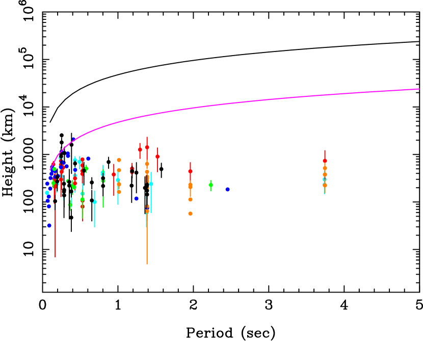
Figure 2: The distribution of radio emission heights with the pulsar period, estimated using the A/R shifts of PPA traverse within the pulsar profile. A total of 71 pulsars are shown in the plot, including the latest measurements from MSPES sample (shown in black) as well as other assorted sources in the literature (red from von Hoensbroech & Xilouris 1997a, green from Mitra & Rankin 2011, blue from Weltevrede & Johnston 2008, cyan from BCW, orange from Mitra & Li 2004). Only data points for which estimated heights are positive and larger than the error bar are shown in the plot. The black points correspond to the MSPES sample of Table 1. The variation of the light cylinder radius (black line) as well as 10% of the light cylinder radius (pink line) with period, are also shown for comparison.

3 Single pulse polarization property

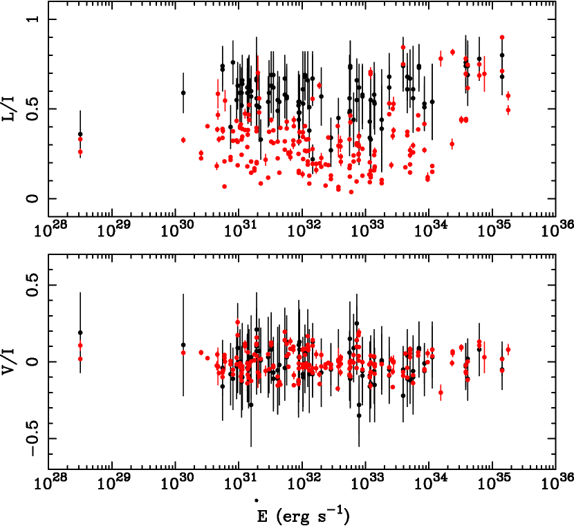
Figure 3: The upper panel shows the variation of fractional linear polarization in AP (red error bars) as well as the mean of the SP linear fractional polarization distribution (black error bars) as a function of $\dot{E}$, for the pulsars observed in MSPES. The corresponding measurements of the fractional circular polarization is shown in the lower panel. The measurements at both observing frequencies, 333 MHz and 618 MHz, are used in these plots.

Figure 4: See caption of Fig 1 for a description of the quantities shown in the figure. The top panels present the polarization behaviour of highly polarized time samples with linear polarization levels greater than 0.8, for PSR J0837+0610 (left panel) and PSR J1752-2806 (right panel). The bottom panels show the corresponding polarization behaviour for weakly polarized time samples with fractional linear polarization levels less than 0.7. The PPA distributions in the top panels are clustered around a narrow track, while they show significantly larger scatter in the bottom panels.

We have used the Hammer-Aitoff projection of the Poincaré sphere to study the distribution of the Stokes parameters for the time samples in the SPs (see bottom panel of Fig 1). This was implemented by selecting time samples of each SP showing significant detection of linear polarization, i.e. polarization intensity being greater than three times the baseline noise rms. The level of polarization is indicated by the colour scheme in each figure and these estimates were carried out only in pulsars with sufficient number of significant samples ($>$90) for further statistical analysis. The fractional linear and circular polarization in SP measurements of every pulsar show a wide spread in their distributions, and their mean and rms is reported in Table 2. The mean levels represent the typical values of the polarization fraction in the SP time sample and are compared with the AP properties. In PaperI we found a general tendency for the evolution of the AP fractional linear polarization in the pulsar population, with generally younger and more energetic pulsars showing higher polarization levels compared to slower, older pulsars. We have extended these comparisons to the SP polarization measurements as shown in Fig. 3. The upper panel of the figure shows the mean fractional linear polarization levels from SP (black error bars) along with the fractional linear polarization from AP (red error bars) as a function of $\dot{E}$, while the bottom panel shows the corresponding results for the circular polarization. In pulsars with $\dot{E}<10^{34}$ ergs s^-1 the fractional linear polarization from SP measurements has mean value of 0.57$\pm$0.15 which is significantly higher than the estimates of 0.29$\pm$0.14 from APs. However, in more energetic pulsars, $\dot{E}>10^{34}$ ergs s^-1, the fractional linear polarization levels from both SP and AP appear to be comparable at around 0.75, although we were unable to derive any statistically significant inference from the MSPES observations due to insufficient sample size in this regime. The mean fractional circular polarization are at low levels and roughly similar across the entire $\dot{E}$ range, with mean values of 0.08$\pm$0.2 for the SP measurements and 0.06$\pm$0.23 for the AP measurements, respectively. The estimated errors are greater than the mean fractional circular polarization since the measurements show large spread within the pulsar population.

The difference in the linear polarization between the SP and AP levels can be associated with the process of estimating the AP polarization from the SPs. This involves first averaging the Stokes parameters $U$ and $Q$ over all SPs and then estimating the linear polarization for every phase bin in the pulse window. Finally, the linear polarization is average across the emission window of the profile. In the process there is significant depolarization in the APs arising from incoherent summation of the highly polarized time samples spread out in the PPAs, and adding time samples with weaker polarization level. A comparison between the SP and AP fractional polarization levels provides several important clues about the radio emission process. Fig 3 (top panel) clearly shows that the differences between the mean SP fractional linear polarization between the low and high energetic pulsars are less prominent compared to the AP measurements. This indicates that the intrinsic emission process primarily produces highly polarized radio emission at shorter timescales. There are more time samples in SPs with low fractional polarization for lower $\dot{E}$ pulsars, suggesting depolarization before the emission detaches from the pulsar magnetosphere. On the other hand the circular polarization level seems to be independent of either the averaging process or pulsar energetics.

A spread in the PPA distribution of SPs is seen in almost all pulsars. In certain cases that have high $\dot{E}$, the time samples in SPs have high levels of linear polarization and the corresponding PPAs are tightly distributed around a mean level. An example of such behaviour from PSR J0742$-$2822 is shown in the left panel of Fig. 1. In case of pulsars with low $\dot{E}$ the linearly polarized time samples have a wider spread and their corresponding PPA traverse can show two different types of behaviour. In the first case the PPAs exhibit highly disordered patterns with wide spread in the distribution of their linear polarization level, such as the behaviour of PSR J1752$-$2806 shown in the middle panel of Fig. 1. In the second case the PPAs are clustered around two parallel tracks, that are separated by 90$\arcdeg$ in phase, as seen in PSR J0034$-$0731 in the right panel of Fig. 1. In several pulsars it was shown that the PPAs corresponding to the high linearly polarized time samples for all three categories follow the RVM nature (Mitra et al., 2009, 2023). A remarkable result was obtained using the MSPES observations of PSR J1645$-$0317 with disordered PPA distribution by Mitra et al. (2023). It was seen that in a subset of the PPA distribution, comprising of only the high linearly polarized time samples, a S-shaped PPA traverse was recovered that followed the RVM. We have expanded these studies to other pulsars in the MSPES sample having disordered PPA distributions, with two examples shown in Fig. 4 corresponding to PSR J0837+0610 (left panel) and PSR J1752$-$2806 (right panel). The top panels show PPA distributions comprising of time samples with fractional linear polarization levels greater than 0.8, and are tightly confined within a narrow region with little spread. The PPA distribution of PSR J0837+0610 clearly follows the RVM, but the RVM nature is still unclear in case of PSR J1752$-$2806. The bottom panels show the PPA distribution made up of time samples with weaker polarization signals at levels less than 0.7, and have a large spread.

Table 2: The measurements of the average fractional SP polarization are presented. Column 1, 2 and 3 correspond to the Jname, observing frequency and spindown energy loss as $\dot{E}_{31}=\dot{E}/10^{31}$ ergs s^-1, respectively. Column 4 presents the number of time samples in the SP sequence that were above the detection threshold and used for the polarization estimates. Columns 5, 6 and 7 reports the mean fractional linear polarization, the mean circular polarization and mean of absolute circular polarization, respectively.

PSR	Freq	$\dot{E_{31}}$	Nsamples	L/I	V/I	$\mid V\mid$/I
J0034$-$0721	333	1.92	26292	0.52 $\pm$ 0.14	0.21 $\pm$ 0.24	0.24 $\pm$0.24
	618		3702	0.56 $\pm$ 0.15	0.07 $\pm$ 0.28	0.20 $\pm$0.20
J0151$-$0635	333	0.556	162	0.74 $\pm$ 0.11	-0.04 $\pm$ 0.18	0.10 $\pm$0.10
	618		587	0.72 $\pm$0.12	-0.16 $\pm$ 0.22	0.19 $\pm$0.19
J0152$-$1637	333	8.88	2219	0.44 $\pm$0.14	0.11 $\pm$ 0.29	0.22 $\pm$0.22
	618		1241	0.48 $\pm$0.15	0.03 $\pm$ 0.29	0.20 $\pm$0.20
J0304+1932	333	1.91	16569	0.67 $\pm$0.14	0.11 $\pm$ 0.20	0.16 $\pm$0.16
	618		7900	0.66 $\pm$0.24	0.10 $\pm$ 0.21	0.16 $\pm$0.16
J0452$-$1759	333	137	20056	0.58 $\pm$0.18	0.03 $\pm$ 0.18	0.11 $\pm$0.11
	618		2702	0.54 $\pm$0.15	-0.06 $\pm$ 0.21	0.14 $\pm$0.14
J0528+2200	333	3.01	8878	0.59 $\pm$0.18	-0.06 $\pm$ 0.14	0.07 $\pm$0.07
J0543+2329	333	4090	4038	0.74 $\pm$0.14	0.02 $\pm$ 0.13	0.07 $\pm$0.07
	618		3543	0.69 $\pm$0.17	-0.11 $\pm$ 0.14	0.10 $\pm$0.10
J0614+2229	618	6240	281	0.78 $\pm$0.12	0.08 $\pm$ 0.17	0.12 $\pm$0.12
J0629+2415	333	72.8	6617	0.55 $\pm$0.12	0.25 $\pm$ 0.19	0.25 $\pm$0.24
	618		169	0.66 $\pm$0.12	0.14 $\pm$ 0.22	0.16 $\pm$0.16
J0630$-$2834	333	14.6	9427	0.67 $\pm$0.13	-0.07 $\pm$ 0.16	0.11 $\pm$0.11
	618		35268	0.67 $\pm$0.15	-0.08 $\pm$ 0.14	0.10 $\pm$0.10
J0659+1414	333	3810	1433	0.76 $\pm$0.15	-0.02 $\pm$ 0.14	0.08 $\pm$0.08
	618		451	0.74 $\pm$0.15	-0.03 $\pm$ 0.15	0.08 $\pm$0.08
J0729$-$1836	333	564	1392	0.56 $\pm$0.17	-0.06 $\pm$ 0.23	0.17 $\pm$0.17
	618		188	0.61 $\pm$0.24	-0.10 $\pm$ 0.24	0.19 $\pm$0.19
J0738$-$4042	333	121	3714	0.55 $\pm$0.13	-0.14 $\pm$ 0.16	0.15 $\pm$0.19
J0742$-$2822	333	14300	33200	0.68 $\pm$0.10	0.02 $\pm$ 0.11	0.06 $\pm$0.06
	618		16328	0.80 $\pm$0.11	-0.05 $\pm$ 0.13	0.08 $\pm$0.08
J0758$-$1528	618	20.1	97	0.57 $\pm$0.16	-0.07 $\pm$ 0.22	0.16 $\pm$0.16
J0820$-$1350	333	4.38	1320	0.54 $\pm$0.14	-0.02 $\pm$ 0.26	0.19 $\pm$0.19
J0837+0610	333	13	50931	0.38 $\pm$0.15	-0.02 $\pm$ 0.23	0.17 $\pm$0.17
	618		6084	0.51 $\pm$0.14	-0.08 $\pm$ 0.25	0.19 $\pm$0.19
J0922+0638	333	697	2840	0.73 $\pm$0.13	0.09 $\pm$ 0.17	0.11 $\pm$0.11
	618		2628	0.74 $\pm$0.12	0.08 $\pm$ 0.18	0.12 $\pm$0.12
J0944$-$1354	333	0.963	516	0.63 $\pm$0.13	0.09 $\pm$ 0.29	0.21 $\pm$0.21
J0953+0755	333	56	64345	0.56 $\pm$0.24	0.06 $\pm$ 0.14	0.10 $\pm$0.10
	618		84594	0.48 $\pm$0.24	-0.09 $\pm$ 0.16	0.13 $\pm$0.13
J1034$-$3224	333	79.1	1531	0.35 $\pm$0.16	-0.35 $\pm$ 0.20	0.35 $\pm$0.35
	618		614	0.62 $\pm$0.13	-0.28 $\pm$ 0.19	0.26 $\pm$0.26
J1041$-$1942	618	1.4	927	0.59 $\pm$0.17	0.00 $\pm$ 0.24	0.17 $\pm$0.17
J1116$-$4122	333	37.4	176	0.45 $\pm$0.11	0.01 $\pm$ 0.20	0.12 $\pm$0.12
J1136+1551	333	8.79	5572	0.54 $\pm$0.17	-0.13 $\pm$ 0.23	0.20 $\pm$0.20
	618		4946	0.52 $\pm$0.17	-0.12 $\pm$ 0.21	0.17 $\pm$0.17
J1239+2453	333	1.43	33204	0.63 $\pm$0.16	-0.09 $\pm$ 0.21	0.17 $\pm$0.17
	618		6241	0.62 $\pm$0.16	-0.05 $\pm$ 0.21	0.14 $\pm$0.14
J1328$-$4921	333	0.745	848	0.40 $\pm$0.12	-0.08 $\pm$ 0.20	0.16 $\pm$0.16
J1527$-$3931	333	5.33	1120	0.58 $\pm$0.13	0.14 $\pm$ 0.21	0.18 $\pm$0.18
	618		160	0.67 $\pm$0.13	-0.04 $\pm$ 0.21	0.12 $\pm$0.12
J1559$-$4438	317	237	788	0.68 $\pm$0.13	-0.05 $\pm$ 0.21	0.14 $\pm$0.14
	618		20858	0.62 $\pm$0.12	-0.09 $\pm$ 0.18	0.14 $\pm$0.14
J1625$-$4048	618	0.134	95	0.59 $\pm$0.11	0.11 $\pm$ 0.33	0.23 $\pm$0.23
J1645$-$0317	618	121	36693	0.33 $\pm$0.19	-0.01 $\pm$ 0.18	0.13 $\pm$0.13
J1703$-$3241	333	1.46	3165	0.64 $\pm$0.14	0.02 $\pm$ 0.19	0.14 $\pm$0.14
	618		3644	0.66 $\pm$0.14	-0.04 $\pm$ 0.22	0.15 $\pm$0.15
J1709$-$1640	333	89.4	17632	0.57 $\pm$0.18	-0.09 $\pm$ 0.17	0.14 $\pm$0.14
	618		1881	0.58 $\pm$0.16	-0.06 $\pm$ 0.22	0.15 $\pm$0.15
J1720$-$2933	618	12.3	124	0.66 $\pm$0.16	0.09 $\pm$ 0.25	0.19 $\pm$0.19
J1731$-$4744	333	1130	21120	0.54 $\pm$0.21	0.08 $\pm$ 0.18	0.14 $\pm$0.14
	618		25042	0.54 $\pm$0.21	0.03 $\pm$ 0.20	0.14 $\pm$0.14
J1735$-$0724	333	65	4287	0.44 $\pm$0.15	0.09 $\pm$ 0.22	0.19 $\pm$0.19
J1740+1311	333	11.1	1805	0.68 $\pm$0.13	0.06 $\pm$ 0.18	0.13 $\pm$0.13
	618		3384	0.69 $\pm$0.13	-0.01 $\pm$ 0.19	0.12 $\pm$0.12
J1741$-$0840	333	1.05	1735	0.59 $\pm$0.15	0.00 $\pm$ 0.20	0.13 $\pm$0.13
	618		838	0.59 $\pm$0.16	0.00 $\pm$ 0.21	0.12 $\pm$0.12
J1741$-$3927	618	56.7	360	0.49 $\pm$0.14	0.15 $\pm$ 0.24	0.20 $\pm$0.20
J1745$-$3040	333	849	144	0.51 $\pm$0.13	-0.01 $\pm$ 0.13	0.12 $\pm$0.12
	618		4237	0.53 $\pm$0.15	-0.06 $\pm$ 0.16	0.13 $\pm$0.13
J1751$-$4657	333	9.11	19827	0.48 $\pm$0.14	0.13 $\pm$ 0.19	0.17 $\pm$0.17
	618		5509	0.54 $\pm$0.15	0.08 $\pm$ 0.26	0.19 $\pm$0.19
J1752$-$2806	333	180	35973	0.39 $\pm$0.24	0.00 $\pm$ 0.18	0.13 $\pm$0.13
	618		53938	0.44 $\pm$0.28	0.01 $\pm$ 0.22	0.16 $\pm$0.16
J1801$-$2920	333	10.3	313	0.61 $\pm$0.21	-0.08 $\pm$ 0.24	0.18 $\pm$0.18
J1817$-$3618	333	139	683	0.53 $\pm$0.17	-0.15 $\pm$ 0.24	0.23 $\pm$0.23
J1820$-$0427	333	117	9973	0.34 $\pm$0.10	-0.16 $\pm$ 0.23	0.24 $\pm$0.24
	618		3208	0.43 $\pm$0.13	-0.09 $\pm$ 0.22	0.17 $\pm$0.17
J1822$-$2256	618	0.812	181	0.76 $\pm$0.12	-0.11 $\pm$ 0.20	0.15 $\pm$0.15
J1823+0550	333	2.1	555	0.51 $\pm$0.19	0.07 $\pm$ 0.21	0.16 $\pm$0.16
J1823$-$3106	333	504	2964	0.67 $\pm$0.16	-0.12 $\pm$ 0.15	0.15 $\pm$0.15
J1900$-$2600	333	3.52	12408	0.62 $\pm$0.17	-0.11 $\pm$ 0.21	0.17 $\pm$0.17
	618		2039	0.69 $\pm$0.13	-0.07 $\pm$ 0.23	0.16 $\pm$0.16
J1901$-$0906	333	1.14	1671	0.64 $\pm$0.13	-0.10 $\pm$ 0.21	0.17 $\pm$0.17
	618		190	0.66 $\pm$0.14	-0.03 $\pm$ 0.28	0.19 $\pm$0.19
J1909+1102	333	457	638	0.61 $\pm$0.13	0.04 $\pm$ 0.17	0.14 $\pm$0.14
	618		91	0.68 $\pm$0.13	-0.11 $\pm$ 0.18	0.13 $\pm$0.13
J1913$-$0440	333	28.5	4960	0.27 $\pm$0.09	-0.02 $\pm$ 0.13	0.09 $\pm$0.09
	618		7026	0.34 $\pm$0.11	-0.05 $\pm$ 0.17	0.13 $\pm$0.13
J1919+0021	333	14.7	783	0.22 $\pm$0.08	0.13 $\pm$ 0.12	0.14 $\pm$0.14
J1921+2153	618	2.23	36710	0.33 $\pm$0.11	0.01 $\pm$ 0.21	0.15 $\pm$0.15
J1932+1059	333	393	36794	0.74 $\pm$0.12	-0.22 $\pm$ 0.17	0.22 $\pm$0.22
	618		20016	0.75 $\pm$0.15	-0.05 $\pm$ 0.15	0.09 $\pm$0.09
J1941$-$2602	333	57.5	118	0.74 $\pm$0.14	-0.11 $\pm$ 0.18	0.13 $\pm$0.13
	618		635	0.73 $\pm$0.15	-0.11 $\pm$ 0.19	0.15 $\pm$0.15
J1946+1805	333	1.11	9953	0.52 $\pm$0.14	-0.09 $\pm$ 0.18	0.14 $\pm$0.14
	618		4822	0.59 $\pm$0.14	-0.13 $\pm$ 0.23	0.19 $\pm$0.19
J2006$-$0807	333	0.927	303	0.55 $\pm$0.12	-0.03 $\pm$ 0.21	0.12 $\pm$0.12
J2046$-$0421	333	1.57	17322	0.57 $\pm$0.16	0.03 $\pm$ 0.27	0.21 $\pm$0.21
	618		2805	0.60 $\pm$0.14	-0.28 $\pm$ 0.27	0.30 $\pm$0.30
J2048$-$1616	333	5.73	114821	0.57 $\pm$0.18	0.13 $\pm$ 0.17	0.16 $\pm$0.16
	618		68016	0.56 $\pm$0.17	0.03 $\pm$ 0.18	0.11 $\pm$0.11
J2144$-$3933	333	0.00318	14763	0.36 $\pm$0.13	0.19 $\pm$ 0.26	0.22 $\pm$0.22
J2305+3100	333	2.92	5543	0.54 $\pm$0.14	0.03 $\pm$ 0.26	0.19 $\pm$0.19
J2313+4253	333	10.4	8555	0.53 $\pm$0.15	-0.10 $\pm$ 0.19	0.15 $\pm$0.15
J2317+2149	333	1.37	1564	0.62 $\pm$0.16	-0.04 $\pm$ 0.22	0.14 $\pm$0.14
	618		207	0.59 $\pm$0.14	-0.01 $\pm$ 0.18	0.11 $\pm$0.11
J2330$-$2005	333	4.12	40307	0.49 $\pm$0.16	-0.11 $\pm$ 0.23	0.19 $\pm$0.19
	618		1921	0.55 $\pm$0.16	-0.55 $\pm$ 0.28	0.20 $\pm$0.20
J2346$-$0609	333	3.26	3035	0.63 $\pm$0.15	0.10 $\pm$ 0.22	0.16 $\pm$0.16
	618		432	0.69 $\pm$0.13	0.08 $\pm$ 0.22	0.16 $\pm$0.16

4 A model for the formation of polarization properties of pulsars.

We have currently accrued significant observational constraints on the radio emission mechanism. The location of the source has been mapped out to be well inside the magnetosphere, at heights below 10% of the light cylinder radius (see section 2). In addition to the limitations on the height of emission the observed polarization behavior makes further demands on the nature of the mechanism. The observed radio waves show high level of linear polarization with the polarization position vector being either perpendicular or parallel to the plane in which the curved dipolar magnetic field lines lie. The emission is also around 10-20 % circularly polarized (see section  2 and  3).

In general, the polarization feature of a pulsar is initially defined by the emission mechanism, and then evolves as the excited wave mode propagate through the magnetosphere. The radio emission should be generated due to some plasma processes and should correspond to the eigenmodes of the magnetospheric plasma, which consists of dense electron-positron pair plasma streaming relativistically outwards in the open magnetic field line region. Generally, pulsar radio emission mechanisms can be divided into two classes, maser mechanisms and antenna mechanisms (Ginzburg & Zhelezniakov, 1975; Ruderman & Sutherland, 1975; Melikidze et al., 2000; Kazbegi et al., 1991). In maser mechanisms the radio emission is generated by certain plasma instabilities that can excite plasma waves capable of escaping the pulsar magnetosphere. The antenna mechanisms on the other hand relies on the coherent curvature radiation (CCR) being the main source of the radio waves. It is therefore essential to understand all possible instabilities that can develop in a relativistic pair plasma in pulsar magnetospheric conditions.

In the radio emission region the magnetic field geometry is dipolar and is still very strong, i.e. the ratio between plasma and cyclotron frequencies $\sigma\ll 1$ here $\sigma={\omega_{p}}/{\omega_{B}}=2\times 10^{-4}\times\kappa^{0.5}\mathcal{R}^{1.5}({P^{3}}/{\dot{P}_{-15}})^{0.25}$, $\mathcal{R}=r/R_{lc}$ with $r$ being the distance and $R_{lc}$ the light cylinder radius, and $\dot{P}_{-15}$ is the period derivative in the units of $10^{-15}$ s s^-1 (see Appendix A). At the emission altitude, $r\simeq 50r_{\ast}$, where $r_{\ast}=10^{6}$ cm is the neutron star radius, $\mathcal{R}\approx 0.01P^{-1}$. At this distance most of the plasma instabilities are suppressed and only the two-stream instability (i.e. the wave-particle interaction at the Cherenkov resonance), can develop. However, $\sigma$ increases with distance as $\mathcal{R}^{1.5}$ and some other instabilities, like cyclotron and/or Cherenkov drift instabilities, can grow near the light cylinder.

If the distribution functions of both plasma components, i.e. electrons and positrons, are identical, the system of dispersion equations is divided into two parts, describing the so called ordinary (O-mode) and extraordinary (X-mode), orthogonally polarized modes of the magnetized pair plasma. We follow the the nomenclature of Shapakidze et al. (2003) to describe the eigen modes in the plasma. The polarization vector of O-mode lies in the plane of $\vec{k}$ and $\vec{B}$ and it has a component along the ambient magnetic field as well as along the propagation vector, $\vec{k}$. The X-mode has a purely non-potential nature and its polarization vector is directed perpendicular to plane containing $\vec{k}$ and $\vec{B}$. There are two additional branches of the O-mode, $lt_{1}$-mode and $lt_{2}$-mode, both having a mixed longitudinal-transverse nature. In case of strictly parallel propagation with respect to the external magnetic field, i.e. $\vec{k}\parallel\vec{B}$, the $lt_{2}$-mode coincide with the Langmuir mode and have purely potential character. The second branch of O-mode, i.e. the $lt_{1}$-mode, as well as X-mode have characteristics of purely transverse waves of arbitrary polarization. The phase velocity of $lt_{1}$-mode is always sub-luminal while $lt_{2}$-mode is super-luminal for relatively small values of the wave vectors and can be sub-luminal at higher frequencies. In case of the frequencies that fall into radio-band the X-mode has one sub-luminal branch and it always has a non-potential nature. The direction of the polarization vectors of the X-mode and O-mode are specified by the plane containing $\vec{k}$ and the local magnetic field, while the polarization vector of observed radio waves are perpendicular to the plane of curved dipolar field lines. Therefore, the emission mechanism should distinguish this plane. In our opinion the only mechanism which can fulfill these requirements is the coherent curvature radiation (CCR). There are indeed several observational evidences for CCR to be the likely emission mechanism for radio emission in pulsars, like the presence of highly polarized subpulses that follow the mean RVM (Mitra et al., 2009), spectral shape variation across the pulse profile (Basu et al., 2022b), etc. Multiple studies have demonstrated that the stable charge bunches capable of exciting CCR can be associated with charge solitons, that can form due to the nonlinear growth of plasma instability in relativistically flowing non-stationary pulsar plasma (Melikidze & Pataraia, 1980; Asseo & Melikidze, 1998; Melikidze et al., 2000; Lakoba et al., 2018; Rahaman et al., 2020; Manthei et al., 2021; Rahaman et al., 2022b).

4.1 The PSG model and plasma parameters

The non-stationary plasma flow in pulsars is generated in an inner accelerating region (IAR) above the polar cap. Ruderman & Sutherland (1975, hereafter RS75) was the first to propose the existence of an IAR for pulsars where $\vec{\Omega}\cdot\vec{B}<0$ above the polar cap, here $\vec{\Omega}$ is the angular velocity of the neutron star and $\vec{B}$ is the local magnetic field. As the outflowing plasma leaves along the open magnetic field lines, the surface ions, that are expected to have large binding energies, cannot be pulled out to screen the large co-rotational electric fields, leading to the formation of an inner vacuum gap (IVG) with large electric potential drop along it. Further, due to the presence of strong and curved magnetic fields above the polar cap electron-positron pairs can be produced in the IAR that are subsequently accelerated to relativistic speeds, such that pair cascades ensue to form a relativistic plasma flow (Sturrock, 1971, RS75). This process is called spark formation and in general several isolated sparks can exist above the polar cap depending on its size. The sparks grow laterally till a size $h$ and screens the electric potential drop within the sparking region, with the next spark forming at a distance $h$ away. Thus a system of isolated sparks are produced, where the center of the spark and the boundary between two sparks are associated with high and low potential drop, respectively. When there is enough charges produced during cascading, the plasma screens the entire electric field, thereby halting the sparking process. The plasma generated during sparking gradually flows out of the IAR, such that the electric potential drop reappears and the the sparking process repeats. This results in a non-stationary spark associated plasma flow and at emission heights of about 50$r_{\ast}$ the coherent radio emission is generated due to instabilities in this outflowing plasma. The emerging radiation associated with each sparking column is seen as subpulses within the pulse emission window. The sparks in the IAR undergo a gradual $\vec{E}\times\vec{B}$ drift motion at longer timescales that is observed as the phenomenon of subpulse drifting. During the sparking process the electric field in the IAR separates the electron-positron pairs, with the electrons accelerated towards the surface and thus heating the polar cap. The positrons which form the primary beam accelerate away from the star with Lorentz factors $\gamma_{p}$, and produces additional cascades of secondary pairs with Lorentz factors $\gamma_{s}$.

The polar cap temperatures estimated from the IVG model of RS75 is higher than the measured values, while the estimated subpulse drift speeds from the RS75 model are faster than those derived from the observed drifting periodicities. This led Gil et al. (2003, hereafter GMG03) to propose a modified IVG model, known as the partially screened gap (PSG), where they postulated the presence of thermally ejected ions in the IAR that can partially screen the electric field, the possibility of which was also discussed earlier by Cheng & Ruderman (1977, 1980). In the PSG model the number density of ions, $n_{ion}$, with respect to the Goldreich-Julien number density, $n_{GJ}$, is estimated as $n_{ion}/n_{GJ}\approx\exp\left[30(1-T_{i}/T_{s})\right]$, where $T_{i}$ is the temperature corresponding to the binding energy of ⁵⁶Fe₂₆ ions and $T_{s}$ is the surface temperature. Since $n_{ion}$ has an exponential dependence on temperature, if $T_{s}$ goes slightly below $T_{i}$ almost vacuum like conditions will appear in the gap, while $T_{s}=T_{i}$ implies a fully screened gap. GMG03 suggested that under thermostatic conditions the surface temperature of the polar cap is slightly lower than $T_{i}$, such that $T_{s}=T_{i}(1-\delta)$, where $\delta$ is a small temperature offset parameter, $\delta\approx 10^{-3}$. Thus unlike the IVG, the PSG never attains a fully vacuum state, and the potential difference in the gap is screened by a factor $\eta=1-n_{ion}/n_{GJ}\approx 0.1$, with ions usually contributing about 90% of $n_{GJ}$. The sparking process in the PSG commences in a manner similar to the IVG model where a set of tightly packed equidistant sparks are produced. The potential drop is maximum at the center of the spark, where the pair multiplicity is largest, and reduces gradually towards the boundary between sparks, which is mostly filled up by diffusion of particles from surrounding sparks, and can be approximated to have a multiplicity factor of unity. The maximum potential drop is obtained as $\eta\Delta V_{vac}=\eta(2\pi B_{s}/cP)h^{2}$, where $\Delta V_{vac}$ is the potential difference of the IVG, $h$ is the gap height and $B_{s}$ the value of surface magnetic field. The sparks grows in size radially with the temperature below it increasing, till it reaches a maximum size when $T_{s}=T_{i}$ and the sparking process ceases. The sparking restarts once the the plasma column, also referred to as plasma cloud, leaves the gap such that $T_{s}<T_{i}$ and once again the potential drop develops, thus giving rise to the non-stationary plasma flow. The lateral size of the sparks, $h_{\perp}$, and the total number of sparks, $N_{sp}$, in the gap at any given time can be estimated as (Mitra et al., 2020; Basu et al., 2020b, 2022a) :

$$h_{\perp}\simeq 15~{}~{}\frac{T_{6}^{2}}{\eta b(\cos{\alpha_{l}})^{1/2}}{\dot{E}_{32}}^{-1/2}P^{-1}~{}~{}~{}{\rm m,}$$

$$N_{sp}\simeq 20~{}\frac{\eta b^{1/2}\cos{\alpha_{l}}}{T_{6}^{2}}(\dot{E}_{32}P)^{1/2}.$$ (3)

Here, $T_{6}=T_{s}/10^{6}K$, $b=B_{s}/B_{d}$, where $B_{s}$ is the non-dipolar field in the surface and $B_{d}$ the equivalent dipolar field, $\alpha_{l}$ is the angle between the local magnetic field and the rotation axis, and $\dot{E}_{32}=\dot{E}\times 10^{-32}$ erg s^-1.

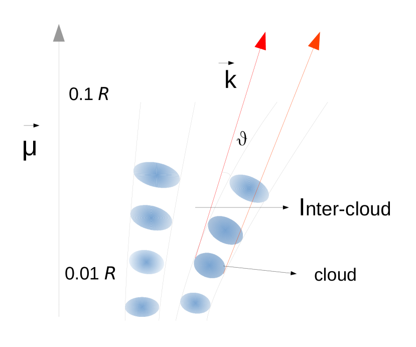
Figure 5: The above cartoon shows the open magnetic field line of a pulsar between heights of 0.01$\mathcal{R}$ and 0.1$\mathcal{R}$, that correspond to radio emission region. The grey lines depict the dipolar magnetic field lines and the shaded blue correspond to plasma clouds. A series of plasma clouds move along the open magnetic field lines due to the non-stationary flow setup by the sparking discharges in the IAR. The white background correspond to the inter-cloud region where the plasma density is lower. CCR is excited in plasma clouds and the propagation vector $\vec{k}$ is depicted as solid red lines. The waves escape to the inter-cloud region above 0.1$\mathcal{R}$ to eventually reach the observer. $\vec{k}$ makes an angle $\vartheta$ with respect to the local dipole magnetic field, $\vec{B}$, given by Eq. 4. $\vec{\mu}$ correspond to the dipole magnetic axis.

GMG03 used observational constraints to estimate $\eta\approx 0.1$ and $T_{s}\approx 2\times 10^{6}$ K. Associating $T_{s}$ with the bombardment of electrons at the polar cap surface, an estimate for the Lorentz factor of the positron beam can be obtained as $\gamma_{p}^{sp}\sim 10^{6}$, where the superscript ‘$sp$’ specifies the sparking region. The positron beam further cascades and produces secondary pairs with multiplicity $\kappa^{sp}$. Several pair cascade simulations suggest $\kappa^{sp}\sim 10^{4}$, and this gives an estimate for the secondary pair plasma Lorentz factor as $\gamma_{s}^{sp}\sim\gamma_{p}^{sp}/2\kappa^{sp}\sim 10^{2}$. Since the ions are much heavier, the corresponding Lorentz factor for the ions are $\gamma_{ion}^{sp}\approx 10^{3}$. In the inter-spark region the potential has a minimum value $\Delta V_{min}$ and there is no pair discharge. GMG03 estimated $\Delta V_{min}$ which accelerates the ion in the inter-spark region to characteristic Lorentz factor of $\gamma_{ion}^{isp}\sim 10$ (see Appendix B), here superscript ‘$isp$’ specifies the inter-spark region. In the inter-spark region the pair plasma is produced primarily from stray high energy photons and has $\kappa^{isp}\sim 1$ and $\gamma_{s}^{isp}\sim 10^{2}$. Each spark associated plasma column consists of intermittently outflowing dense plasma clouds along the open, curved, dipolar magnetic field lines. Thus the radio emission region alternates between dense plasma clouds and low density inter-cloud region (see Fig. 5).

Figure 6: The angle between the propagation vector, $\vec{k}$, and the local magnetic field $\vec{B}$, is represented by $\vartheta$, and its variation with altitude, $\mathcal{R}$, is shown in the left panel (see Eq. 4). The altitude is represented in terms of the light cylinder radius and we assume the emission to originate at $\mathcal{R}_{1}=0.01$ where $\vartheta=0$. The right panel shows the altitude evolution of resonance frequency of the pair plasma, $\nu_{res,p}$ (dashed red line, Eq. 7), the resonance frequency of ions, $\nu_{res,ion}$ (blue line, Eq. 7) and the emission frequency excited by CCR, $\nu_{r}$ (red line, Eq. 8). The shaded area (in yellow) represents the region from which the radio emission can be generated, with the radio frequency range typically between 20 MHz and 10 GHz (horizontal dashed lines).

4.2 The origin of the nature of pulsar polarization

The CCR from charge bunches (or solitons) are excited inside the dense pair-plasma clouds at distances of about 1% of the light cylinder radius. The Lorentz factors of solitons have the same order of magnitude as $\gamma_{s}^{sp}$, with CCR exciting the $lt_{1}$-mode and $t$-mode at the radio frequency range, $\nu_{cr}<2\sqrt{\gamma_{s}^{sp}}\nu_{p}^{sp}$. The plasma modes are linearly polarized and oriented parallel and perpendicular to the magnetic field planes, respectively. The power in the $t$-mode is seven times smaller than the $lt_{1}$-mode. The refractive indices of the two modes are different and they split and propagate as independent modes through the plasma clouds. The $t$-mode has vacuum like properties in the dense plasma clouds and can escape as electromagnetic X-mode to reach the observer. On the other hand the magnetic field lines act like ducts for the $lt_{1}$-mode to propagate along them, and it eventually undergoes Landau damping. As a result the $lt_{1}$-mode cannot escape a homogeneous plasma. However, if large density gradients exist such that in regions of lower pair multiplicity the condition $\nu_{cr}>2\sqrt{\gamma_{s}^{sp}}\nu_{p}^{sp}$ is satisfied, then the $lt_{1}$-mode is able escape and reach the observer. This is precisely the nature of the non-stationary plasma flow in pulsars that originates from a PSG, and near the boundary of the clouds both the $t$-mode and $lt_{1}$-mode escape into the inter-cloud region as X-mode and O-mode, respectively.

In the wave generation region, located well inside the pulsar magnetosphere, the wave vector $\vec{k}$ is directed almost tangent to the magnetic field lines, i.e. the angle between them $\vartheta\simeq 0$, while the opening angle of a single charge bunch is about $1/\gamma_{s}^{sp}$. As the magnetic field lines are curved, $\vartheta$ increases with distance as the waves propagate and when $\vartheta>1/\gamma_{s}^{sp}$ the emission enters the inter-cloud region where the plasma density is lower. The resultant emission has contribution from a large number of charge bunches inside the dense plasma column, such that the angular size of the profile component, having typical widths of around 2°, can be associated with the width of the plasma column. We use polar co-ordinates ($\mathcal{R}$, $\theta$) to specify the wave generation region, where $\mathcal{R}$ is defined in terms of light cylinder radius. If the location of the wave generation point, where $\vec{k}\parallel\vec{B}_{1}$, is specified as ($\mathcal{R}_{1}$, $\theta_{1}$), such that $\vartheta_{1}=0$, then at an altitude $\mathcal{R}$ the angle $\vartheta$ is given as (see Appendix C)

$$\vartheta=\frac{3}{4}\left[\theta_{1}-2\sin^{-1}\left(\frac{\mathcal{R}_{1}}{\mathcal{R}}\sin{\cfrac{\theta_{1}}{2}}\right)\right].$$ (4)

The variation of $\vartheta$ with $\mathcal{R}$ obtained from Eq. 4 is shown in Fig. 6 (left panel). At an altitude of $\mathcal{R}=0.1R_{lc}$ (10% of the light cylinder radius), $\vartheta\approx 0.07$ radian or about $4^{\circ}$, which is greater than the profile component widths. This clearly suggests that around 20% of light cylinder radius $\vartheta$ is large enough for the emission to enter the inter-cloud region (see cartoon in Fig. 5).

Once the waves enter the inter-cloud region, both the X-mode and the O-mode propagate following the dispersion relation of the $t$-mode, $\omega=kc(1-\omega_{p}^{2}/4\gamma^{3}\omega_{B}^{2})$. The waves can undergo Čerenkov as well as cyclotron damping, with the resonance condition of the form,

$$\omega_{res}-\vec{k}.{\vec{v}}-\frac{1}{\gamma}\omega_{B}=0$$ (5)

Here $\omega_{res}$ is the resonance frequency and $\vec{v}$ is the velocity of the resonant particles that are confined to move along the local magnetic field. Using the dispersion relation of the $t$-mode the resonance condition can be used to find the resonance frequency,

$$\nu_{res}=\frac{\omega_{B}}{2\pi\gamma}\left(\frac{\vartheta^{2}}{2}+\frac{1}{2\gamma^{2}}-\frac{\omega_{p}^{2}}{4\gamma^{3}\omega_{B}^{2}}\right)^{-1}$$ (6)

where we have used $\vec{k}\cdot\vec{v}=kv\cos{\vartheta}=kc(1-\vartheta^{2}/2-1/2\gamma^{2})$. The resonance frequency of the pair plasma, $\nu_{res,p}$, and ions, $\nu_{res,ion}$, in the inter-cloud region as a function of $\mathcal{R}$ is given as

$$\nu_{res,p} = \frac{1.69\times 10^{5}}{\mathcal{R}^{3}(2.45\times 10^{-3}-3.76\times 10^{-16}\mathcal{R}^{3})}~{}~{}\rm{GHz},$$

$$\nu_{res,ion} = \frac{1.273\times 10^{-6}}{\mathcal{R}^{3}(7\times 10^{-3}-4.06\times 10^{-8}\mathcal{R}^{3})}~{}~{}\rm{GHz}.$$ (7)

Here, typical values of the parameters $P=\dot{P}_{-15}=1$ was used, and in the inter-cloud region $\gamma_{s}^{isp}=300$, $\kappa^{isp}=1$ for the pair plasma, while $\gamma_{ion}^{isp}=10$ for ions.

If the frequency of CCR, $\nu_{r}$, coincide with the resonance frequency then they will undergo damping. Inside the plasma cloud the condition for the emission of radio frequencies can be expressed in terms of $\mathcal{R}$ as,

$$\nu_{r}<2\sqrt{\gamma_{s}^{sp}}\nu_{p}=0.035/\mathcal{R}^{1.5},$$ (8)

where typical values of the pair plasma, $\kappa^{sp}=10^{4}$ and $\gamma_{s}^{sp}=300$, have been used. The change in resonance frequencies (Eq. 7) as well as the characteristic plasma frequency (Eq. 8), with $\mathcal{R}$, have been shown in Fig. 6 (right panel), where the shaded area (in yellow) specifies the radio emission region within the magnetosphere. At distances above 0.1$\mathcal{R}$ the broadband pulsar radiation can detach from the dense plasma cloud and propagate in the inter-cloud region. The resonance conditions shown in Fig. 6 indicate that the plasma waves can travel a large distance in the inter-cloud region before crossing the resonance point. Mikhailovskii et al. (1982) showed that in a homogeneous plasma the waves generated inside the magnetosphere will undergo cyclotron damping and cannot escape the pulsar. However, when inhomogeneity is introduced in the plasma, as explained above, the resonance condition only becomes applicable higher up in the pulsar magnetosphere for the waves propagating in the inter-cloud region. In the upper magnetosphere the pair plasma density decreases significantly and hence the effect of damping will be much smaller. In this work we have used a a static dipole model, which is not adequate for describing the magnetic field structure in the upper magnetosphere, where magnetic sweep-back effects dominate. Therefore, a comprehensive analysis of the damping effects will require a more detailed model of the upper magnetosphere and will be addressed in future studies.

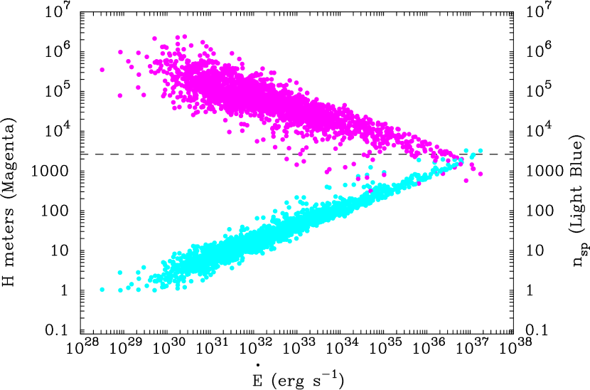
Figure 7: The change in the inter-cloud separation with $\dot{E}$ is shown for pulsars with $P>0.1$ s (Magenta). These estimates are carried out at the typical emission height $r=50r_{\ast}$ (see Eq. 9). The figure also shows the variation of number of sparks, $N_{sp}$, and as an extension the number of plasma columns in the open field line region, as a function of $\dot{E}$ (light blue). In the low $\dot{E}$ range the estimated $N_{sp}$ is less than unity in certain pulsars, and has been approximated as a single spark in the plot. The charge bunches in the plasma clouds emit within a narrow cone with angular size $(3/2)(1/\gamma_{s}^{sp})$. The horizontal line (dashed) shows the linear extension of the emission cone at $50r_{\ast}$.

4.3 Origin of Linear Polarization

We propose that the observed linear polarization features in pulsars arise due to incoherent addition of the X-mode and O-mode of CCR, excited by the large number of charge bunches in the plasma clouds. The $t$-mode can easily escape from the inter-cloud region and appear as the X-mode with high levels of linear polarization (see Rahaman et al. 2022a). The $lt_{1}$-mode, which is seven times stronger than $t$-mode, is mostly damped inside the plasma cloud, but can also escape as a dominant mode from the inter-cloud boundary region as the linearly polarized O-mode (Arons & Barnard 1986; Gil et al. 2004; Melikidze et al. 2014). At any instant of time there are multiple plasma clouds that emit X-mode and O-mode with different intensities, that undergo incoherent averaging in the inter-cloud region. This process gives us the resultant linear polarization and the PPA distribution observed from pulsars and depends on the level of inhomogeneity in the magnetospheric plasma.

A measure of the inhomogeneity in the plasma comes from the spark size, $h_{\perp}$, and number of sparks, $N_{sp}$, in the PSG. Eq. 3 gives an estimate of $h_{\perp}$ and $N_{sp}$ as well as their variation in the pulsar population, specified by the dependence on $\dot{E}$. The inter-cloud separation, $H$, in the emission region $r$ can be calculated from $h_{\perp}$ at the surface $r_{\ast}$ as :

$$H=bh_{\perp}\left(\frac{r}{r_{\ast}}\right)^{1.5}$$ (9)

Fig. 7 shows the variation of $H$ (magenta), estimated at $50r_{\ast}$, and $N_{sp}$ (light blue) with $\dot{E}$ for normal pulsars with $P\geq 0.1$ s. We have used typical parameters of a PSG, $\eta=0.1$, $b=10$, $T_{6}=2$, $\alpha_{m}=45\arcdeg$, for these estimates, and the pulsar parameters were obtained from the ATNF pulsar database (Manchester et al., 2005). $N_{sp}$ increases significantly with $\dot{E}$, ranging from one expected spark at 10²⁹ erg s^-1 to around 10³ sparks at 10³⁶ erg s^-1, while $H$ has a decreasing trend ranging from 10⁶ m to 10³ m over the same range of $\dot{E}$. The charge bunches emit CCR tangential to the curved magnetic field lines over a narrow cone with angular extent $(3/2)(1/\gamma_{s}^{sp})$ rad. The size of the emission cone at $50r_{\ast}$ is around 2000 m (horizontal line in Fig. 7) and lies below $H$ for almost the entire population.

In low $\dot{E}$ pulsars, with lower number of plasma clouds and larger separation between them, once the emission enters the inter-cloud region there is sufficient gap for the $lt_{1}$-mode to escape without getting damped by encountering another plasma cloud. For example PSR J0034$-$0721 shown in Fig. 1 has low $\dot{E}\sim 1.9\times 10^{31}$ ergs/s and the estimated $H\sim 1.3\times 10^{6}$ m and $N_{sp}\sim 8$, and clearly the gap size is orders of magnitude larger than the emission cone. As a result both $t$-mode and $lt_{1}$-mode can escape as X-mode and O-mode and give rise to the orthogonal PPA traverse that follow the RVM, similar to what is observed in PSR J0034$-$0721. In contrast, high $\dot{E}$ pulsars have large number of closely packed clouds and have higher likelihood of absorbing the $lt_{1}$-mode. The situation here can be applied to PSR J0742$-$2822 of Fig. 1 with $\dot{E}=1.4\times 10^{35}$ ergs/s. The estimated $H\sim 8400$ m is of the same order of the emission cone thus reducing the gap for escape of $lt_{1}$-mode and further $N_{sp}\sim 308$ is large. Thus in this case only highly polarized time samples with a single PPA traverse following the RVM are observed. In certain intermediate cases it is possible for both $t$-mode and $lt_{1}$-mode to escape as X-mode and O-mode from plasma clouds which add up incoherently and show large variation in the degree of polarization with significant spread in PPA distribution. PSR J1752$-$2806 shown in Fig. 1 with $\dot{E}=1.8\times 10^{33}$ ergs/s correspond to such a case. The estimated $H\sim 2\times 10^{5}$ m falls in the middle range compared to above two cases, and $N_{sp}\sim 63$. In this situation it appears that mode mixing can occur as observed in Fig. 1. The above model also predicts that the PPA from highly polarized time samples should follow the RVM, that have been identified in certain pulsars (Mitra et al., 2009, 2023). Incoherent averaging of CCR due to a large number of coherently emitting single charge bunches has also been explored in earlier studies to explain the observed depolarization and corresponding PPA behaviour (Gil & Rudnicki, 1985; Gil & Snakowski, 1990). Our present scheme involves a more consistent model of plasma clouds emerging from sparks in a PSG, with several other implications, like high surface temperatures in the polar cap region, presence of non-dipolar fields near the stellar surface, subpulse drifting of sparks, etc., and have various degrees of observational verifications. However, understanding the full spectrum of the observed polarization features using this model requires detailed simulations, which will be explored in a separate study.

4.4 Circular Polarization as a propagation effect

The circularly polarized waves require additional conditions that can break the symmetry between the positive and negative components of the electron-positron pair plasma. This can likely be realised from the small differences in the distribution functions of electrons and positrons as well as the presence of small amounts of positively charged Iron ions in the plasma. Kazbegi et al. (1991, hereafter KMM91) used the difference in distribution functions of pair plasma to explain the presence of circularly polarized modes. We use the standard textbook definitions to investigate the percentage circular polarization in plasma waves (see e.g. Shafranov, 1967). We have used a co-ordinate system where one axis is directed along the propagation vector, $\vec{k}$, and electric vector is of the form $\vec{E}=E_{y}(ia_{x},1,ia_{z})$, here $a_{x}$ governs the polarization of the waves. The dispersion relation in this system is given as

$$a_{x}^{2}-\Theta a_{x}-1=0,$$

$$\Theta=\cfrac{\left(\eta-1\right)+g^{2}}{g\eta\cos\vartheta}\sin^{2}\vartheta,$$ (10)

here, $\vartheta$ is the angle between $\vec{k}$ and $\vec{B}$, while $\eta$ and $g$ depend on the parameters of the plasma (see Appendix D). The solution of this equation has the form

$$a_{x}=\frac{1}{2}\Theta\pm\sqrt{\left(\frac{1}{2}\Theta\right)^{2}+1}.$$ (11)

When $\Theta\ll 1$ then $a_{x}\simeq\pm 1$ and there is circular polarization, while $\Theta\gg 1$ implies either $a_{x}=0$ or $a_{x}\gg 1$ and there are two linearly polarized waves.

In the model proposed by KMM91 the radio emission is generated near the light cylinder, around the last open field lines, and the waves leave the magnetosphere immediately after their emission, such that their polarization properties are preserved. It is clear from Eq. 10 that $\Theta$ is directly dependent on $\vartheta$. As a result in this model the core component, located at the center of the profile, i.e. $\vartheta\ll 1$, should show circular polarization, while the conal components that are located farther away are expected to be linearly polarized. However, this is not adequate to explain the observed circular polarization since the radio emission is excited in the inner inner magnetosphere around 0.01$\mathcal{R}$.

The PSG model gives rise to a system of spark associated plasma clouds where the waves are generated at the emission heights and subsequently enter the inter-cloud region above 0.1$\mathcal{R}$. The multiplicity factor of the pair-plasma density, $\kappa$, shows considerable variation across the cloud and inter-cloud regions, with maximum value at the center of the cloud that decreases monotonically to much lower values in the middle of the inter-cloud region. The Lorentz factor of the ions follow a similar profile, having highest value at cloud center and the lowest in the middle of the inter-cloud region. The wave propagates in the inter-cloud region at an angle $\vartheta\sim 0.07$ rad, which remains constant over large distances in the inner magnetosphere (see Fig. 6). The parameter $\Theta$ has the following form in the inter-cloud region (see Appendix  D)

$$\Theta=-\cfrac{I}{g}\sin^{2}\vartheta=1.8\times 10^{10}~{}\mathcal{R}^{3}\cfrac{\kappa^{isp}}{{(\gamma_{s}^{isp})^{3}}}\left(\cfrac{P^{5}}{\dot{P}_{-15}}\right)^{0.5}\omega_{G}.$$ (12)

Here, $(\gamma_{s}^{isp})^{-3}=\langle 1/(\gamma_{s}^{isp})^{3}\rangle$ is the average Lorentz factor of the electron-positron component of the plasma, and $\omega_{G}$ is the radio frequency in GHz. Using typical parameters of the inter-cloud region at $\mathcal{R}=0.1$, i.e. $\gamma_{s}^{isp}\approx 300$, $\kappa^{isp}=P=\dot{P}_{-15}=\omega_{G}=1$, and assuming $1/\gamma_{ion}^{isp}>\sin\vartheta$, we obtain the absolute value $\mid\Theta\mid\approx 0.67$. We can estimate $\mid\Theta\mid$ for the three pulsars shown in Fig. 1, using similar values for $\mathcal{R}\sim 0.1$, $\gamma_{s}^{isp}\approx 300$ and $\kappa^{isp}=1$ and the observing frequency $\omega_{G}=0.6.$ Then for younger pulsars PSR J0742$-$2822 (with $P=0.167$ s and $\dot{P}_{-15}=16.8$) and PSR J1752$-$2806 (with $P=0.563$ s and $\dot{P}_{-15}=8.13$ ) value of $\mid\Theta\mid$ is much less then one ($0.001$ and $0.03$ respectively). For relatively older pulsar PSR J0034$-$0721 (with $P=0.943$ s and $\dot{P}_{-15}=0.408$) $\mid\Theta\mid\sim 0.5$ . Thus, it can be seen that the necessary condition for circular polarization $\mid\Theta\mid\ll 1$ can be easily satisfied for each case.

The above discussion shows that the electromagnetic waves passing through the inter-cloud region will be elliptically polarized, with the degree of polarization depending on the values of $a_{x}$. If $a_{x}=1$ then the waves should have 100% circular polarization, while for either smaller or bigger values of $a_{x}$ the level of linear polarization increases. The observed levels of circular polarization will ultimately depend on the multiplicity profile between the inter-cloud region and incoherent addition of the elliptically polarized emission from several plasma clouds, with the sign of the circular polarization depending on the viewing geometry.

5 Conclusion

We have carried out a systematic analysis of the AP and SP polarization properties of the normal pulsar population observed in MSPES. We have estimated the radio emission heights in several cases using the A/R method and found the radio emission to arise below 10% of the light cylinder radius. The emission heights appear to be constant across a wide period range, which is consistent with earlier studies (Mitra, 2017; Posselt et al., 2022). The SP polarization behaviour show that in general the time samples have high levels of linear polarization. The depolarization in AP arises due to incoherent addition of polarized time samples from the SP, resulting in significant spread of the PPA distributions. The average percentage linear polarization from SP do not show significant variation across the $\dot{E}$ range, which is in sharp contrast with the AP polarization levels, where high $\dot{E}$ pulsars have much higher levels of linear polarization compared to lower $\dot{E}$ cases. The percentage of circular polarization on the other hand do not show any significant variations between the SP and AP measurements.

There is increasing observational evidence that the radio emission arises due to CCR from charge bunches in the outflowing plasma. The charge bunches develop in clouds of plasma formed due to sparking discharges in a PSG, and is primarily composed of dense electron-positron pair plasma, mixed with small amounts of relativistic iron ions, with varying densities and Lorentz factor in the plasma clouds and inter-cloud regions. We have explored the origin of the observed polarization behaviour due to CCR from charge bunches in this plasma configuration. The relativistic charge bunches can excite the $t$-mode and $lt_{1}$-mode that have linear polarizations directed perpendicular and parallel to the curved dipolar magnetic field line planes, respectively. The resultant emission from the plasma cloud is due to incoherent averaging of emission from a large number of charge bunches. The $t$-mode and $lt_{1}$-mode escape into the inter-cloud region at around 10% of the light cylinder radius, where the pair multiplicity is much lower as the ions have smaller Lorentz factors. The modes can propagate as electromagnetic waves corresponding to the X-mode and O-mode, and further incoherent averaging takes place. We show that the waves remains in the inter-cloud region with the angle between the propagation vector almost reaching a constant value, and due to propagation effects the modes attain elliptical polarization below 20% of the light cylinder radius. As the plasma density decreases with height, the waves are eventually able to escape the magnetosphere from the inter-cloud region and reach the observer. However, the magnetic field sweep-back effects become important at heights above 50% of the light cylinder radius and introduce effects like cyclotron damping, which requires more detailed considerations.

Appendix A Some useful definitions

The plasma frequency $\omega_{p}$ and cyclotron frequency $\omega_{B}$ in electron positron plasma is given as

$$\omega_{p} = \sqrt{\frac{4\pi{q_{e}}^{2}n}{m_{e}}}$$ (A1)

$$= 6.4151\times 10^{4}~{}\kappa^{0.5}\mathcal{R}^{-1.5}P^{-1.75}\dot{P}_{15}^{0.25}$$ (A2)

Here the number density $n=\kappa n_{GJ}$, where $n_{GJ}$ is the Goldreich-Julien density.

$$\omega_{B} = \frac{eB}{m_{e}c}$$ (A3)

$$= 3.1834\times 10^{8}~{}\mathcal{R}^{-3}P^{-2.5}{\dot{P}_{15}}^{0.5}$$ (A4)

Estimates of the plasma frequency corresponding to ions, $\omega_{p,ion}$, and the cyclotron frequency, $\omega_{B,ion}$, using ${}^{56}Fe_{26}$,

$$\omega_{p,ion} = 1.02\times 10^{3}~{}\mathcal{R}^{-1.5}P^{-1.75}{\dot{P}_{-15}}^{0.25}$$ (A5)

$$\omega_{B,ion} = 8\times 10^{4}~{}\mathcal{R}^{-3}P^{-2.5}{\dot{P}_{-15}}^{0.5}$$ (A6)

Appendix B Lorentz factor of ⁵⁶Fe₂₆ ions in inter-spark region

In the inter-spark region the gap potential decreases and as a result the Lorentz factors of the outflowing plasma is lower. A minimum potential $\Delta V_{min}$ can be defined where the sparking discharge terminates and the Lorentz factor of the ions ${}^{56}Fe_{26}$ can be written as,

$$\gamma_{Fe}=\Delta V_{\min}\left(\cfrac{26q_{e}}{56m_{p}c^{2}}\right)$$ (B1)

In the PSG model an estimate of $\Delta V_{min}\approx 10^{8}$ V was obtained by Gil et al. (2003), and the minimum Lorentz factor required for pair production dominated by inverse Compton scattering at near threshold condition was (see appendix A.1 therein)
$\gamma_{Fe}=10^{8}\left(\cfrac{26q_{e}}{56m_{p}c^{2}}\right)\sim 14$.

Appendix C Evolution of propagation angle

At the emission region $\vec{k}$ is almost parallel to local $\vec{B}$. It means that in the wave generation region, which is defined as a region which corresponds to $r=r_{1}$ and $\theta=\theta_{1},$ angle between $k$ and $\vec{B}$ is about $0$, here $r$ is radial distance in the units of the stellar radius. The angle $\zeta$ between $\vec{k}$ and magnetic axes $\vec{\mu}$ is $\zeta=\frac{3}{2}\theta_{1}=\frac{3}{2}\theta_{p}r_{1}^{0.5}$, here $\theta_{p}=1.4477\times 10^{-2}P^{-0.5}$ is a coordinate of the last open field line at $r_{1}=1$. The radio waves propagate along $\vec{k}$ (let us note that this direction does not coincide with radius vector direction) and thus we need to calculate the angle $\vartheta$ between $\vec{k}$ and local magnetic field direction at some altitude $(r,\theta)$. In spherical coordinates the equation of the line in the plane of the curved magnetic field plane can be expressed as

$$r\cos\theta=ar\sin\theta+b$$ (C1)

Here at $r_{1}$,

$$a=\cot\cfrac{3}{2}\theta_{1}$$ (C2)

$$b=r_{1}\left[\cos\theta_{1}-\cot\left(\frac{3\theta_{1}}{2}\right)\sin\theta_{1}\right]=r_{1}~{}\frac{\sin\left(\cfrac{\theta_{1}}{2}\right)}{\sin\left(\cfrac{3\theta_{1}}{2}\right)}$$ (C3)

Then,

$$\vartheta=\cfrac{3}{2}\left(\theta-\theta_{1}\right)=\frac{3}{2}\left[\frac{1}{2}\theta_{1}-\sin^{-1}\left(\frac{r_{1}}{r}\sin\cfrac{\theta_{1}}{2}\right)\right]$$ (C4)

$$\vartheta=\frac{3}{4}\left[\theta_{1}-2\sin^{-1}\left(\frac{\mathcal{R}_{1}}{\mathcal{R}}\sin\cfrac{\theta_{1}}{2}\right)\right].$$ (C5)

Appendix D Estimation of the parameter $\Theta$

We consider a wave with electric field $\vec{E}$ where the propagation vector $\vec{k}$ is directed along $z-$axes and $\vartheta$ is the angle between $\vec{B}$ and $\vec{k}$. To describe the wave polarization we introduce the following notation:

$$\vec{E}=E_{y}\left(ia_{x},1,ia_{z}\right)$$ (D1)

where $ia_{x}$ and $ia_{z}$ are the ratio of the $x$ and $z$ components of $\vec{E}$ to its $y$ component $E_{y}$. Following Shafranov (1967) and Kazbegi et al. (1991) we need to define the coefficients of the equation that describes the wave polarisation as

$$\eta_{xx} = \cfrac{\varepsilon_{1}\eta}{\varepsilon_{1}\sin^{2}\vartheta+\eta\cos^{2}\vartheta}$$ (D2)

$$\eta_{xy} = -\eta_{yx}=i\cfrac{g\eta\cos\vartheta}{\varepsilon_{1}\sin^{2}\vartheta+\eta\cos^{2}\vartheta}$$ (D3)

$$\eta_{yy} = \cfrac{\varepsilon_{2}\left(\varepsilon_{1}\sin^{2}\vartheta+\eta\cos^{2}\vartheta\right)-g^{2}\sin^{2}\vartheta}{\varepsilon_{1}\sin^{2}\vartheta+\eta\cos^{2}\vartheta}$$ (D4)

For the case of plasma in the strong magnetic field $\varepsilon_{1}=\varepsilon_{2}=1$. The coefficients of the permitivity tensor are

$$\eta = 1-\sum\limits_{\alpha}\omega_{p_{\alpha}}^{2}\int\cfrac{f_{\alpha}\left(p\right)}{\gamma^{3}}dp\cfrac{1}{\left(\omega-\vec{k}\vec{v}\right)^{2}}\equiv 1-I$$ (D5)

$$g = \sum\limits_{\alpha}\cfrac{\omega_{p_{\alpha}}^{2}}{\omega^{2}}\int\cfrac{f_{\alpha}\left(p\right)dp}{\gamma}\left(\omega-kv\right)A_{\alpha}^{-}$$ (D6)

$$A_{\alpha}^{-} = \cfrac{1}{\omega-kv+\gamma^{-1}\omega_{B\alpha}}-\cfrac{1}{\omega-kv-\gamma^{-1}\omega_{B\alpha}}$$ (D7)

Here $\alpha$ and $\gamma$ correspond to the species and Lorentz factor of the species and $v$ is the velocity of the plasma.

$$\eta_{xx} = \cfrac{1-I}{1-I\cos^{2}\vartheta}$$ (D8)

$$\eta_{yy} = \cfrac{\sin^{2}\vartheta+\eta\cos^{2}\vartheta-g^{2}\sin^{2}\vartheta}{1-I\cos^{2}\vartheta}$$ (D9)

$$\cfrac{\eta_{xx}-\eta_{yy}}{\eta_{yx}} = \cfrac{-I+g^{2}}{g\eta\cos\vartheta}\sin^{2}\vartheta$$ (D10)

Thus the equation for $a_{x}$ is

$$a_{x}^{2}-\Theta a_{x}-1=0$$ (D11)

Here $\Theta$ is given by,

$$\Theta= \cfrac{\eta_{xx}-\eta_{yy}}{i\eta_{yx}}= \cfrac{\left(\eta-1\right)+g^{2}}{g\eta\cos\vartheta}\sin^{2}\vartheta$$ (D12)

The solution is $a_{x}=\frac{1}{2}\Theta\pm\sqrt{\left(\frac{1}{2}\Theta\right)^{2}+1}$. Now if $\Theta\ll 1$ then $a_{x}\simeq\pm 1,$ so the polarization is circular. If $\Theta\gg 1$ then $a_{x}=0$ or $a_{x}\gg 1$. Thus there are two linearly polarised waves.

In the present case we apply the above theory to determine the effect of propagation in the inter-cloud region where we assume that $\sin\vartheta\gg\left\langle\cfrac{1}{\gamma_{s}^{isp}}\right\rangle$ and $\sin\vartheta<\left\langle\cfrac{1}{\gamma_{ion}^{isp}}\right\rangle.$ Further, in the low density inter-cloud plasma we can assume that the dispersion relation for all waves are electromagnetic, such that $\omega\approx kc$. Thus one can write $\left(\omega^{2}-k^{2}v^{2}\right)=\left(\omega^{2}-k^{2}v^{2}\cos^{2}\vartheta\right)=\omega^{2}\left(\sin^{2}\vartheta+\cfrac{1}{\gamma^{2}}\right)$

Under this assumption $A_{\alpha}^{-}$ is dominated by the ion component, and we can estimate

$$(A_{ion}^{isp})^{-}=8(\gamma_{ion}^{isp})^{3}\cfrac{\omega_{B,ion}}{\omega^{2}}.$$ (D13)

The angle $\vartheta$ in the inter-cloud region is almost constant and $\vartheta\approx 0.07$, and $g$ is dominated by the ion component while $I$ is dominated by the pair plasma. Finally we can estimate $g$ and $I$ (see Appendix A for parameters) as

$$g = 2\left(\cfrac{\omega_{B,ion}~{}\omega_{p,{ion}}^{2}}{\omega^{3}}\right)$$ (D14)

$$I = \cfrac{1}{(\gamma_{s}^{isp})^{3}}\cfrac{\omega_{p}^{2}}{\omega^{2}}\cfrac{4}{\sin^{4}\vartheta}$$ (D15)

Therefore, $\Theta=-\cfrac{I}{g}\sin^{2}\vartheta=17.77~{}\kappa\mathcal{R}^{3}\cfrac{\omega}{(\gamma_{s}^{isp})^{3}}\left(\cfrac{{P}^{5}}{\dot{P}_{-15}}\right)^{0.5}$, and introducing $\omega_{G}=\cfrac{\omega}{10^{9}}$

$$\Theta=-1.8\times 10^{10}~{}\kappa\mathcal{R}^{3}\cfrac{1}{(\gamma_{s}^{isp})^{3}}\left(\cfrac{P^{5}}{\dot{P}_{-15}}\right)^{0.5}\omega_{G}$$ (D16)

Appendix E Supplementary Figures

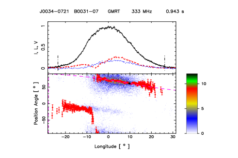
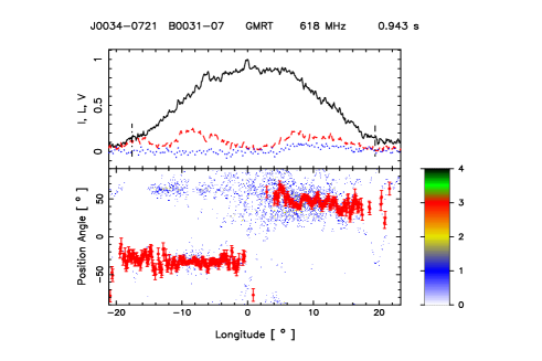
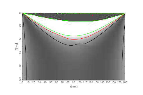
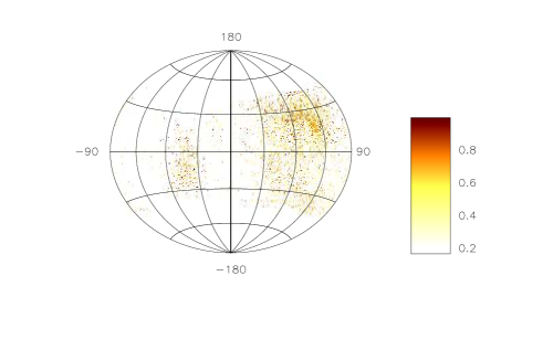
Figure 8: Top panel (upper window) shows the average profile with total intensity (Stokes I; solid black lines), total linear polarization (dashed red line) and circular polarization (Stokes V; dotted blue line). Top panel (lower window) also shows the single pulse PPA distribution (colour scale) along with the average PPA (red error bars). The RVM fits to the average PPA (dashed pink line) is also shown in this plot. Middle panel show the $\chi^{2}$ contours only for 333 MHz and the correlated parameters $\alpha$ and $\beta$ obtained from RVM fits. Bottom panel shows the Hammer-Aitoff projection of the polarized time samples with the colour scheme representing the fractional polarization level.

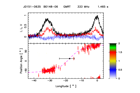
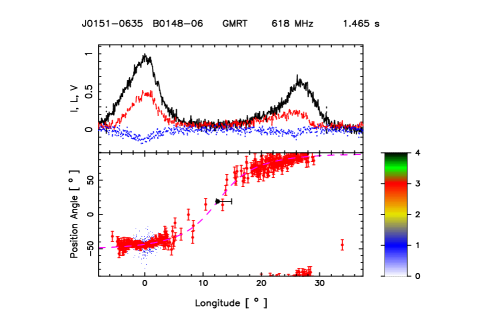
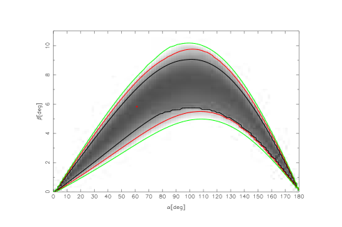
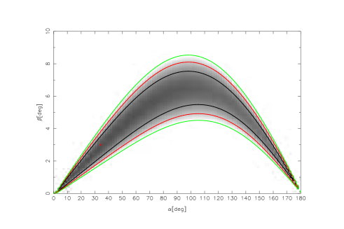
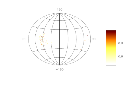
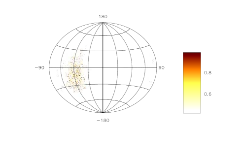
Figure 9: Top panel (upper window) shows the average profile with total intensity (Stokes I; solid black lines), total linear polarization (dashed red line) and circular polarization (Stokes V; dotted blue line). Top panel (lower window) also shows the single pulse PPA distribution (colour scale) along with the average PPA (red error bars). The RVM fits to the average PPA (dashed pink line) is also shown in this plot. Middle panel show the $\chi^{2}$ contours for the parameters $\alpha$ and $\beta$ obtained from RVM fits. Bottom panel shows the Hammer-Aitoff projection of the polarized time samples with the colour scheme representing the fractional polarization level.

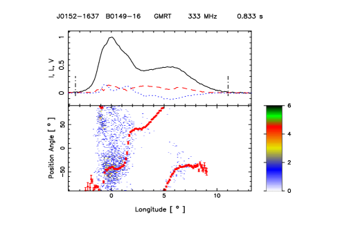
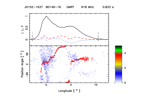
Figure 10: Top panel (upper window) shows the average profile with total intensity (Stokes I; solid black lines), total linear polarization (dashed red line) and circular polarization (Stokes V; dotted blue line). Top panel (lower window) also shows the single pulse PPA distribution (colour scale) along with the average PPA (red error bars). Bottom panel shows the Hammer-Aitoff projection of the polarized time samples with the colour scheme representing the fractional polarization level.

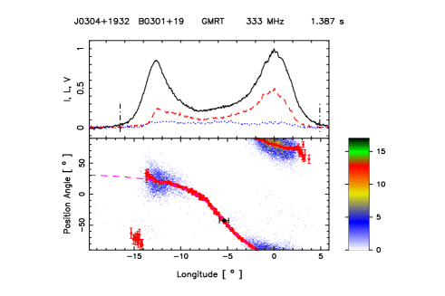
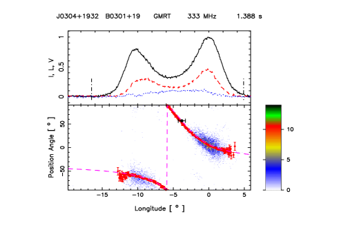
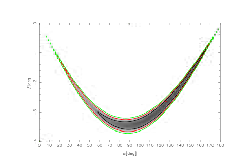
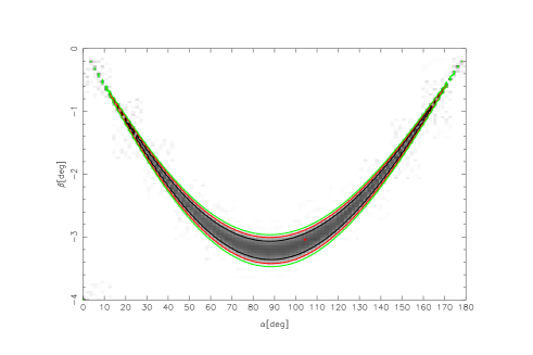
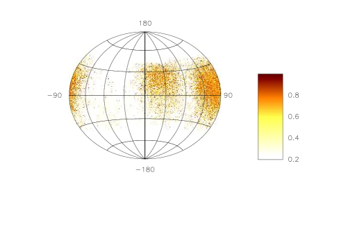
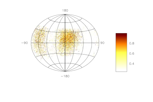
Figure 11: Top panel (upper window) shows the average profile with total intensity (Stokes I; solid black lines), total linear polarization (dashed red line) and circular polarization (Stokes V; dotted blue line). Top panel (lower window) also shows the single pulse PPA distribution (colour scale) along with the average PPA (red error bars). The RVM fits to the average PPA (dashed pink line) is also shown in this plot. Middle panel show the $\chi^{2}$ contours for the parameters $\alpha$ and $\beta$ obtained from RVM fits. Bottom panel shows the Hammer-Aitoff projection of the polarized time samples with the colour scheme representing the fractional polarization level.

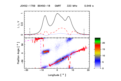
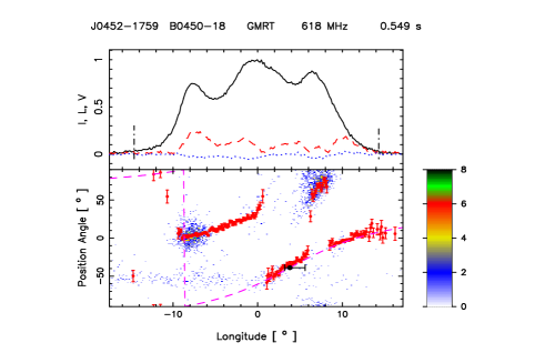
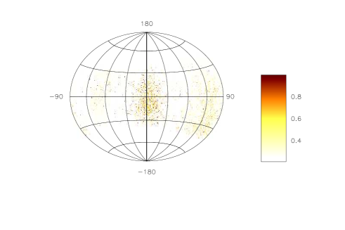
Figure 12: Top panel (upper window) shows the average profile with total intensity (Stokes I; solid black lines), total linear polarization (dashed red line) and circular polarization (Stokes V; dotted blue line). Top panel (lower window) also shows the single pulse PPA distribution (colour scale) along with the average PPA (red error bars). The RVM fits to the average PPA (dashed pink line) is also shown in this plot. Middle panel show the $\chi^{2}$ contours for the parameters $\alpha$ and $\beta$ obtained from RVM fits. Bottom panel shows the Hammer-Aitoff projection of the polarized time samples with the colour scheme representing the fractional polarization level.

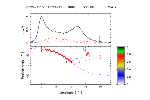
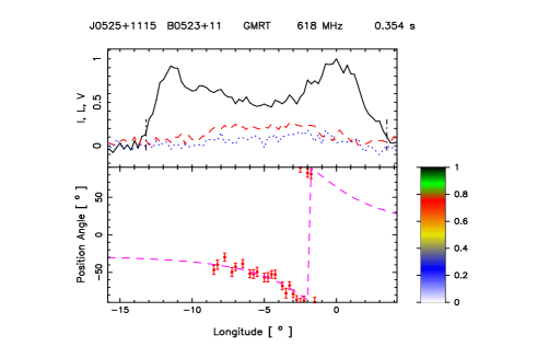
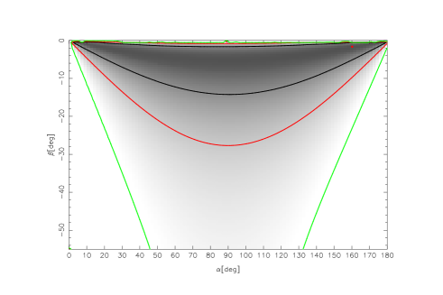
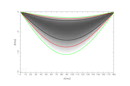
Figure 13: Top panel (upper window) shows the average profile with total intensity (Stokes I; solid black lines), total linear polarization (dashed red line) and circular polarization (Stokes V; dotted blue line). Top panel (lower window) also shows the single pulse PPA distribution (colour scale) along with the average PPA (red error bars). The RVM fits to the average PPA (dashed pink line) is also shown in this plot. Bottom panel show the $\chi^{2}$ contours for the parameters $\alpha$ and $\beta$ obtained from RVM fits.

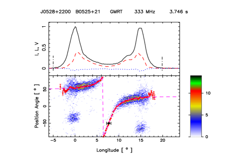
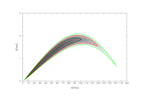
Figure 14: Top panel (upper window) shows the average profile with total intensity (Stokes I; solid black lines), total linear polarization (dashed red line) and circular polarization (Stokes V; dotted blue line). Top panel (lower window) also shows the single pulse PPA distribution (colour scale) along with the average PPA (red error bars). The RVM fits to the average PPA (dashed pink line) is also shown in this plot. Middle panel show the $\chi^{2}$ contours for the parameters $\alpha$ and $\beta$ obtained from RVM fits. Bottom panel shows the Hammer-Aitoff projection of the polarized time samples with the colour scheme representing the fractional polarization level.

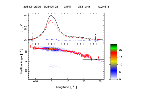
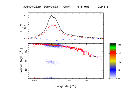
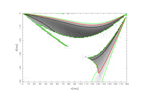
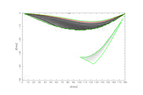
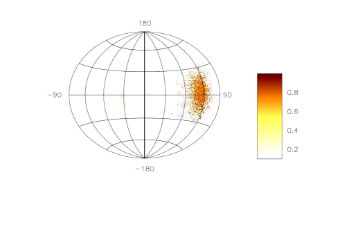
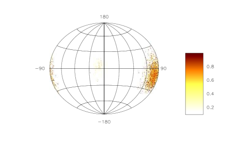
Figure 15: Top panel (upper window) shows the average profile with total intensity (Stokes I; solid black lines), total linear polarization (dashed red line) and circular polarization (Stokes V; dotted blue line). Top panel (lower window) also shows the single pulse PPA distribution (colour scale) along with the average PPA (red error bars). The RVM fits to the average PPA (dashed pink line) is also shown in this plot. Middle panel show the $\chi^{2}$ contours for the parameters $\alpha$ and $\beta$ obtained from RVM fits. Bottom panel shows the Hammer-Aitoff projection of the polarized time samples with the colour scheme representing the fractional polarization level.

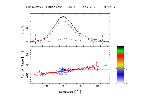
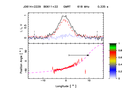
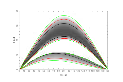
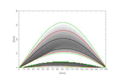
Figure 16: Top panel (upper window) shows the average profile with total intensity (Stokes I; solid black lines), total linear polarization (dashed red line) and circular polarization (Stokes V; dotted blue line). Top panel (lower window) also shows the single pulse PPA distribution (colour scale) along with the average PPA (red error bars). The RVM fits to the average PPA (dashed pink line) is also shown in this plot. Middle panel show the $\chi^{2}$ contours for the parameters $\alpha$ and $\beta$ obtained from RVM fits. Bottom panel only for 333 MHz shows the Hammer-Aitoff projection of the polarized time samples with the colour scheme representing the fractional polarization level.

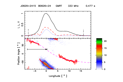
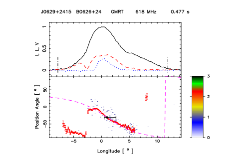
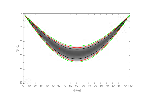
Figure 17: Top panel (upper window) shows the average profile with total intensity (Stokes I; solid black lines), total linear polarization (dashed red line) and circular polarization (Stokes V; dotted blue line). Top panel (lower window) also shows the single pulse PPA distribution (colour scale) along with the average PPA (red error bars). The RVM fits to the average PPA (dashed pink line) is also shown in this plot. Middle panel show the $\chi^{2}$ contours for the parameters $\alpha$ and $\beta$ obtained from RVM fits. Bottom panel shows the Hammer-Aitoff projection of the polarized time samples with the colour scheme representing the fractional polarization level.

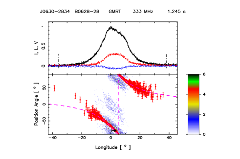
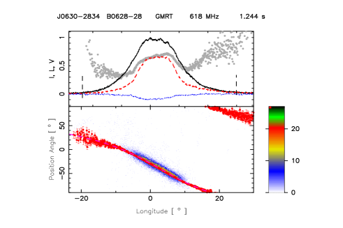
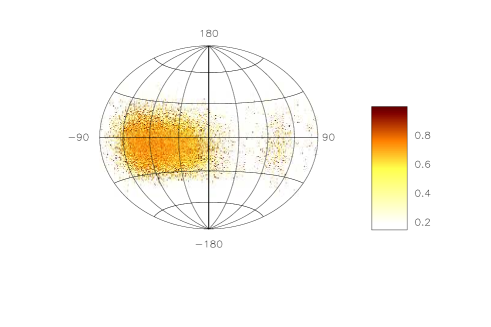
Figure 18: Top panel (upper window) shows the average profile with total intensity (Stokes I; solid black lines), total linear polarization (dashed red line) and circular polarization (Stokes V; dotted blue line). Top panel (lower window) also shows the single pulse PPA distribution (colour scale) along with the average PPA (red error bars). The RVM fits to the average PPA (dashed pink line) is also shown in this plot. Middle panel show the $\chi^{2}$ contours for the parameters $\alpha$ and $\beta$ obtained from RVM fits. Bottom panel shows the Hammer-Aitoff projection of the polarized time samples with the colour scheme representing the fractional polarization level.

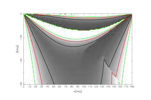
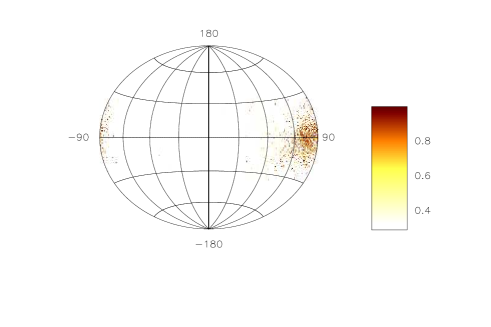
Figure 19: Top panel (upper window) shows the average profile with total intensity (Stokes I; solid black lines), total linear polarization (dashed red line) and circular polarization (Stokes V; dotted blue line). Top panel (lower window) also shows the single pulse PPA distribution (colour scale) along with the average PPA (red error bars). The RVM fits to the average PPA (dashed pink line) is also shown in this plot. Middle panel show the $\chi^{2}$ contours for the parameters $\alpha$ and $\beta$ obtained from RVM fits. Bottom panel shows the Hammer-Aitoff projection of the polarized time samples with the colour scheme representing the fractional polarization level.

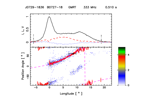
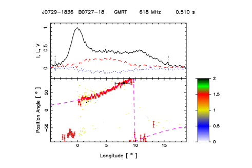
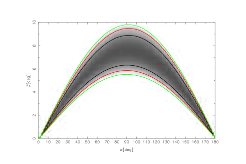
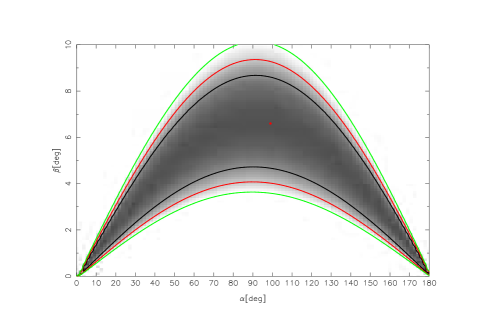
Figure 20: Top panel (upper window) shows the average profile with total intensity (Stokes I; solid black lines), total linear polarization (dashed red line) and circular polarization (Stokes V; dotted blue line). Top panel (lower window) also shows the single pulse PPA distribution (colour scale) along with the average PPA (red error bars). The RVM fits to the average PPA (dashed pink line) is also shown in this plot. Middle panel show the $\chi^{2}$ contours for the parameters $\alpha$ and $\beta$ obtained from RVM fits. Bottom panel shows the Hammer-Aitoff projection of the polarized time samples with the colour scheme representing the fractional polarization level.

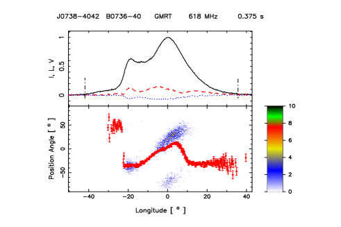
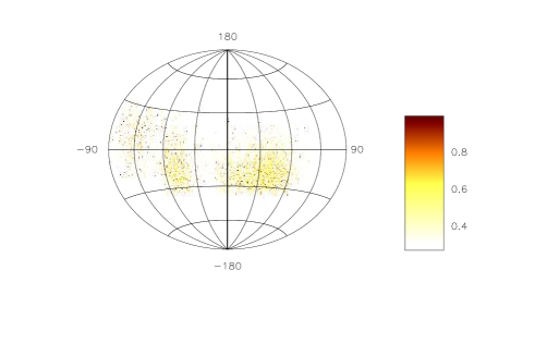
Figure 21: Top panel only for 618 MHz (upper window) shows the average profile with total intensity (Stokes I; solid black lines), total linear polarization (dashed red line) and circular polarization (Stokes V; dotted blue line). Top panel (lower window) also shows the single pulse PPA distribution (colour scale) along with the average PPA (red error bars). Bottom panel only for 618 MHz shows the Hammer-Aitoff projection of the polarized time samples with the colour scheme representing the fractional polarization level.

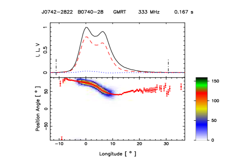
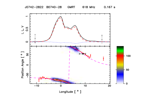
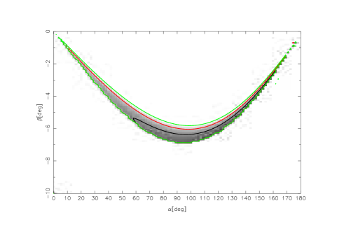
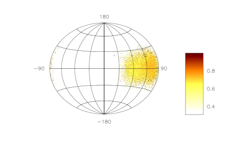
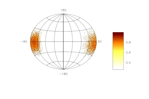
Figure 22: Top panel (upper window) shows the average profile with total intensity (Stokes I; solid black lines), total linear polarization (dashed red line) and circular polarization (Stokes V; dotted blue line). Top panel (lower window) also shows the single pulse PPA distribution (colour scale) along with the average PPA (red error bars). The RVM fits to the average PPA (dashed pink line) is also shown in this plot. Middle panel only for 618 MHz show the $\chi^{2}$ contours for the parameters $\alpha$ and $\beta$ obtained from RVM fits. Bottom panel shows the Hammer-Aitoff projection of the polarized time samples with the colour scheme representing the fractional polarization level.

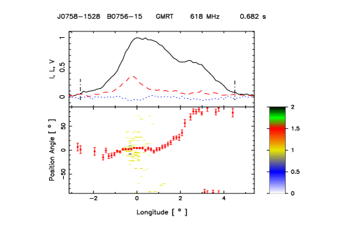
Figure 23: Top panel only for 618 MHz (upper window) shows the average profile with total intensity (Stokes I; solid black lines), total linear polarization (dashed red line) and circular polarization (Stokes V; dotted blue line). Top panel (lower window) also shows the single pulse PPA distribution (colour scale) along with the average PPA (red error bars). Bottom panel shows the Hammer-Aitoff projection of the polarized time samples with the colour scheme representing the fractional polarization level.

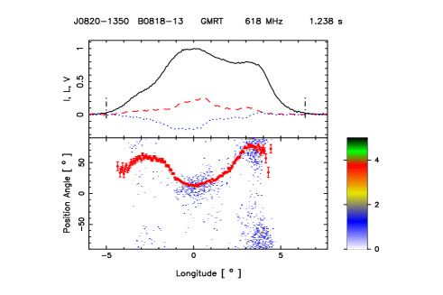
Figure 24: Top panel only for 618 MHz (upper window) shows the average profile with total intensity (Stokes I; solid black lines), total linear polarization (dashed red line) and circular polarization (Stokes V; dotted blue line). Top panel (lower window) also shows the single pulse PPA distribution (colour scale) along with the average PPA (red error bars). Bottom panel shows the Hammer-Aitoff projection of the polarized time samples with the colour scheme representing the fractional polarization level.

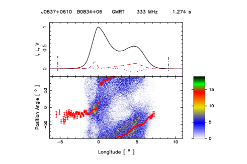
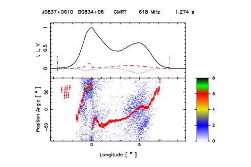
Figure 25: Top panel (upper window) shows the average profile with total intensity (Stokes I; solid black lines), total linear polarization (dashed red line) and circular polarization (Stokes V; dotted blue line). Top panel (lower window) also shows the single pulse PPA distribution (colour scale) along with the average PPA (red error bars). Bottom panel shows the Hammer-Aitoff projection of the polarized time samples with the colour scheme representing the fractional polarization level.

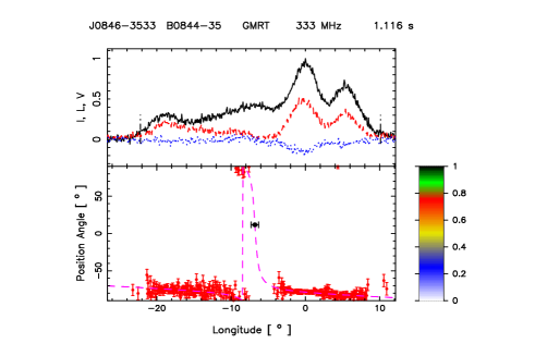
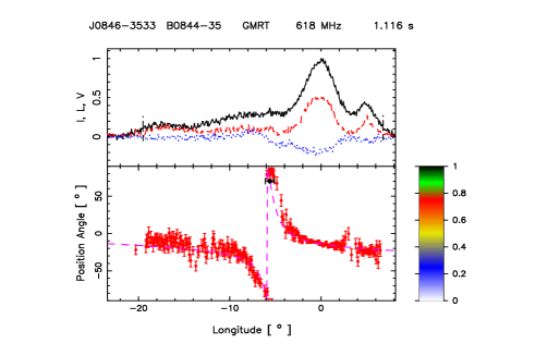
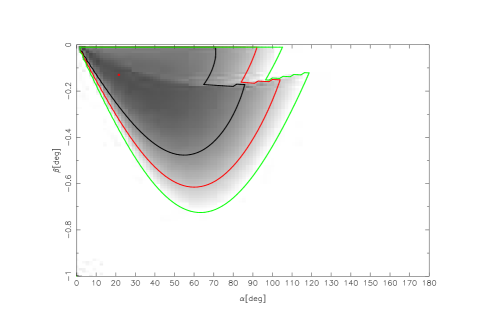
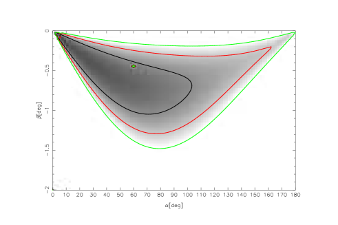
Figure 26: Top panel (upper window) shows the average profile with total intensity (Stokes I; solid black lines), total linear polarization (dashed red line) and circular polarization (Stokes V; dotted blue line). Top panel (lower window) also shows the single pulse PPA distribution (colour scale) along with the average PPA (red error bars). The RVM fits to the average PPA (dashed pink line) is also shown in this plot. Bottom panel show the $\chi^{2}$ contours for the parameters $\alpha$ and $\beta$ obtained from RVM fits.

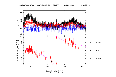
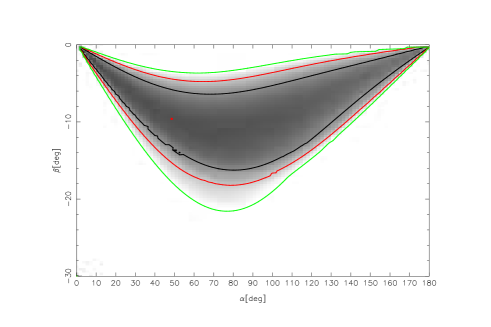
Figure 27: Top panel only for 618 MHz (upper window) shows the average profile with total intensity (Stokes I; solid black lines), total linear polarization (dashed red line) and circular polarization (Stokes V; dotted blue line). Top panel (lower window) also shows the single pulse PPA distribution (colour scale) along with the average PPA (red error bars). The RVM fits to the average PPA (dashed pink line) is also shown in this plot. Bottom panel show the $\chi^{2}$ contours for the parameters $\alpha$ and $\beta$ obtained from RVM fits.

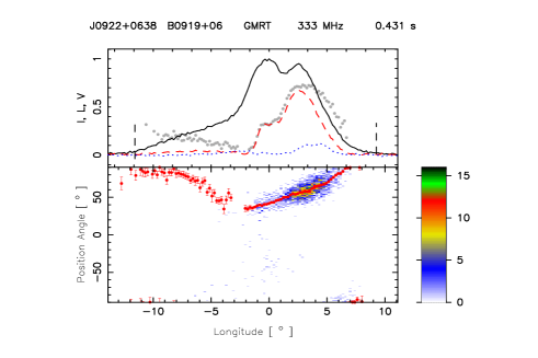
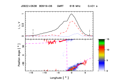
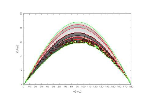
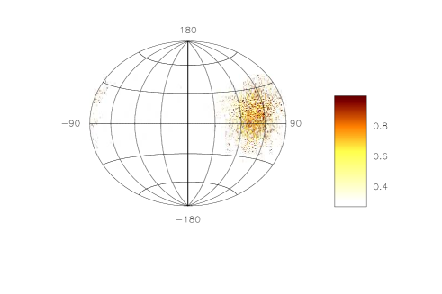
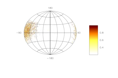
Figure 28: Top panel (upper window) shows the average profile with total intensity (Stokes I; solid black lines), total linear polarization (dashed red line) and circular polarization (Stokes V; dotted blue line). Top panel (lower window) also shows the single pulse PPA distribution (colour scale) along with the average PPA (red error bars). The RVM fits to the average PPA (dashed pink line) is also shown in this plot. Middle panel only for 618 MHz show the $\chi^{2}$ contours for the parameters $\alpha$ and $\beta$ obtained from RVM fits. Bottom panel shows the Hammer-Aitoff projection of the polarized time samples with the colour scheme representing the fractional polarization level.

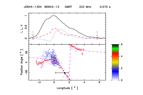
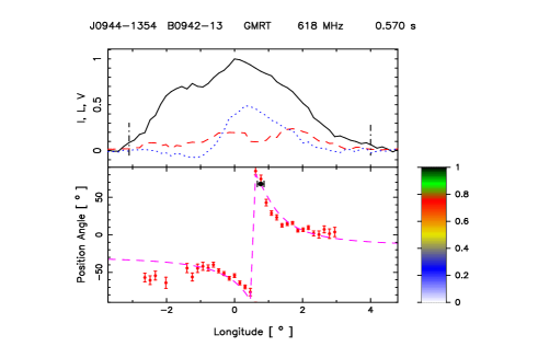
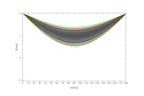
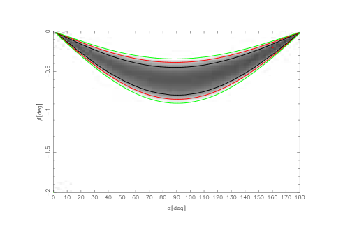
Figure 29: Top panel (upper window) shows the average profile with total intensity (Stokes I; solid black lines), total linear polarization (dashed red line) and circular polarization (Stokes V; dotted blue line). Top panel (lower window) also shows the single pulse PPA distribution (colour scale) along with the average PPA (red error bars). The RVM fits to the average PPA (dashed pink line) is also shown in this plot. Middle panel show the $\chi^{2}$ contours for the parameters $\alpha$ and $\beta$ obtained from RVM fits. Bottom panel only for 333 MHz shows the Hammer-Aitoff projection of the polarized time samples with the colour scheme representing the fractional polarization level.

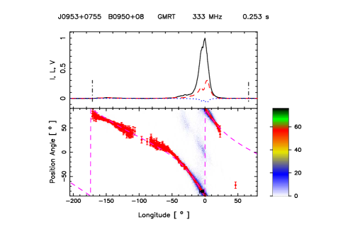
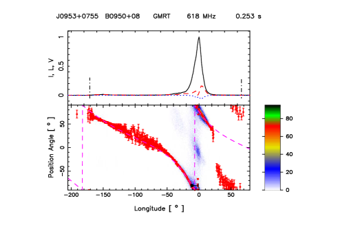
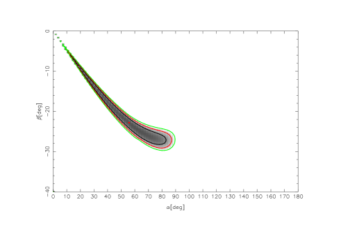
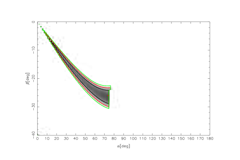
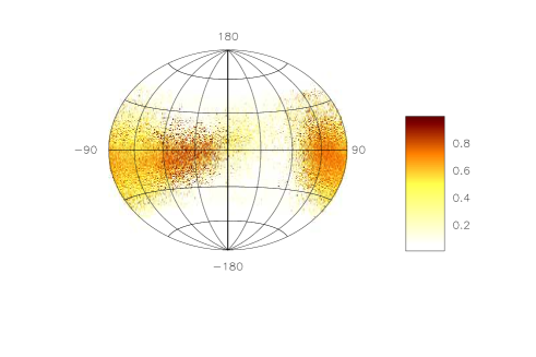
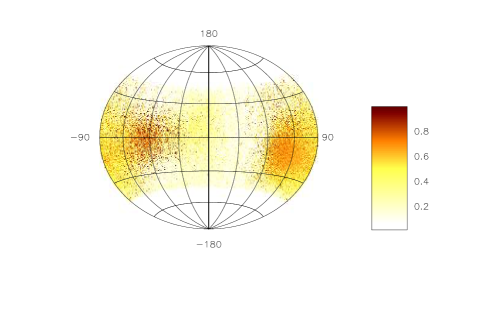
Figure 30: Top panel (upper window) shows the average profile with total intensity (Stokes I; solid black lines), total linear polarization (dashed red line) and circular polarization (Stokes V; dotted blue line). Top panel (lower window) also shows the single pulse PPA distribution (colour scale) along with the average PPA (red error bars). The RVM fits to the average PPA (dashed pink line) is also shown in this plot. Middle panel show the $\chi^{2}$ contours for the parameters $\alpha$ and $\beta$ obtained from RVM fits. Bottom panel shows the Hammer-Aitoff projection of the polarized time samples with the colour scheme representing the fractional polarization level.

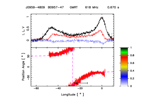
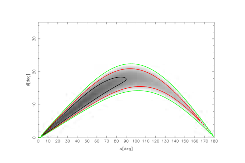
Figure 31: op panel only for 618 MHz (upper window) shows the average profile with total intensity (Stokes I; solid black lines), total linear polarization (dashed red line) and circular polarization (Stokes V; dotted blue line). Top panel (lower window) also shows the single pulse PPA distribution (colour scale) along with the average PPA (red error bars). The RVM fits to the average PPA (dashed pink line) is also shown in this plot. Bottom panel show the $\chi^{2}$ contours for the parameters $\alpha$ and $\beta$ obtained from RVM fits.

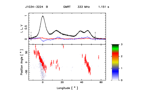
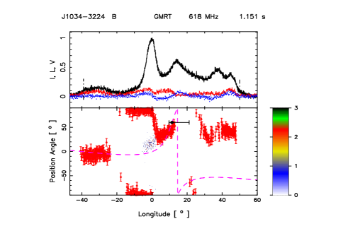
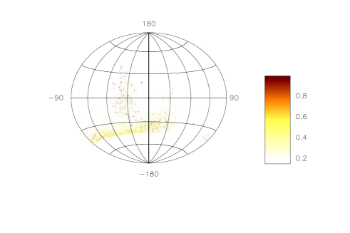
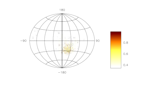
Figure 32: Top panel (upper window) shows the average profile with total intensity (Stokes I; solid black lines), total linear polarization (dashed red line) and circular polarization (Stokes V; dotted blue line). Top panel (lower window) also shows the single pulse PPA distribution (colour scale) along with the average PPA (red error bars). The RVM fits to the average PPA (dashed pink line) is also shown in this plot. Middle panel only for 618 MHz show the $\chi^{2}$ contours for the parameters $\alpha$ and $\beta$ obtained from RVM fits. Bottom panel shows the Hammer-Aitoff projection of the polarized time samples with the colour scheme representing the fractional polarization level.

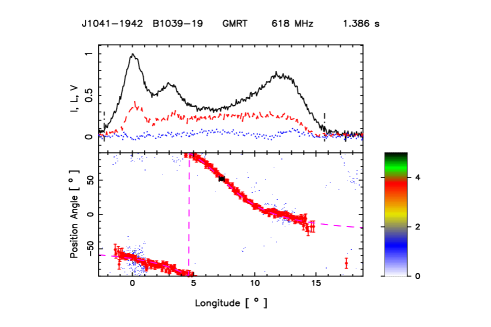
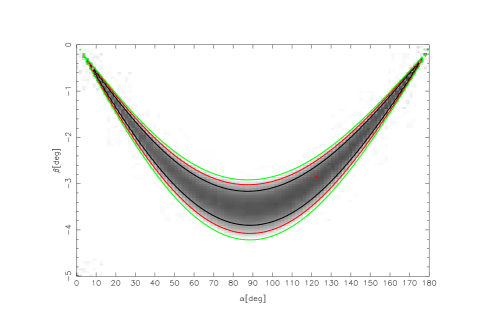
Figure 33: Top panel only for 618 MHz (upper window) shows the average profile with total intensity (Stokes I; solid black lines), total linear polarization (dashed red line) and circular polarization (Stokes V; dotted blue line). Top panel (lower window) also shows the single pulse PPA distribution (colour scale) along with the average PPA (red error bars). The RVM fits to the average PPA (dashed pink line) is also shown in this plot. Middle panel only for 618 MHz show the $\chi^{2}$ contours for the parameters $\alpha$ and $\beta$ obtained from RVM fits. Bottom panel only for 618 MHz shows the Hammer-Aitoff projection of the polarized time samples with the colour scheme representing the fractional polarization level.

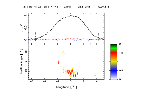
Figure 34: Top panel only for 333 MHz (upper window) shows the average profile with total intensity (Stokes I; solid black lines), total linear polarization (dashed red line) and circular polarization (Stokes V; dotted blue line). Top panel (lower window) also shows the single pulse PPA distribution (colour scale) along with the average PPA (red error bars). Bottom panel only for 333 MHz shows the Hammer-Aitoff projection of the polarized time samples with the colour scheme representing the fractional polarization level.

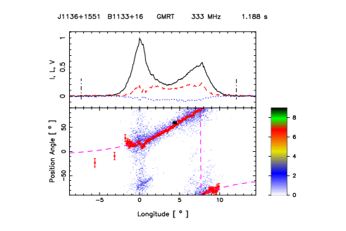
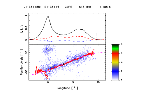
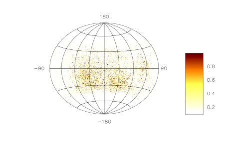
Figure 35: Top panel (upper window) shows the average profile with total intensity (Stokes I; solid black lines), total linear polarization (dashed red line) and circular polarization (Stokes V; dotted blue line). Top panel (lower window) also shows the single pulse PPA distribution (colour scale) along with the average PPA (red error bars). The RVM fits to the average PPA (dashed pink line) is also shown in this plot. Middle panel show the $\chi^{2}$ contours for the parameters $\alpha$ and $\beta$ obtained from RVM fits. Bottom panel shows the Hammer-Aitoff projection of the polarized time samples with the colour scheme representing the fractional polarization level.

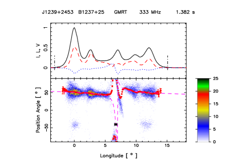
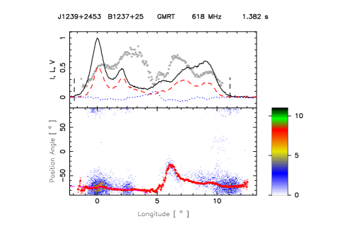
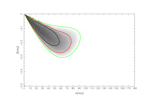
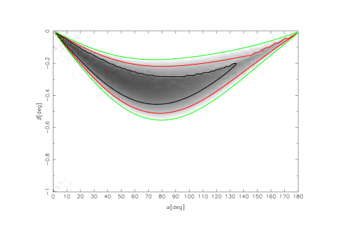
Figure 36: Top panel (upper window) shows the average profile with total intensity (Stokes I; solid black lines), total linear polarization (dashed red line) and circular polarization (Stokes V; dotted blue line). Top panel (lower window) also shows the single pulse PPA distribution (colour scale) along with the average PPA (red error bars). The RVM fits to the average PPA (dashed pink line) is also shown in this plot. Middle panel show the $\chi^{2}$ contours for the parameters $\alpha$ and $\beta$ obtained from RVM fits. Bottom panel shows the Hammer-Aitoff projection of the polarized time samples with the colour scheme representing the fractional polarization level.

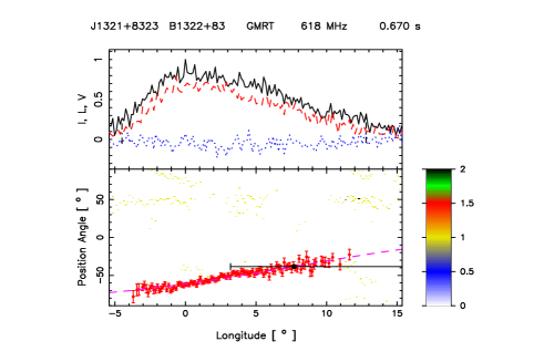
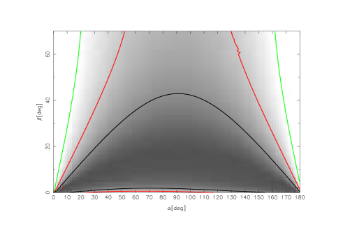
Figure 37: Top panel only for 618 MHz (upper window) shows the average profile with total intensity (Stokes I; solid black lines), total linear polarization (dashed red line) and circular polarization (Stokes V; dotted blue line). Top panel (lower window) also shows the single pulse PPA distribution (colour scale) along with the average PPA (red error bars). The RVM fits to the average PPA (dashed pink line) is also shown in this plot. Bottom panel only for 618 MHz show the $\chi^{2}$ contours for the parameters $\alpha$ and $\beta$ obtained from RVM fits.

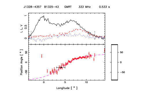
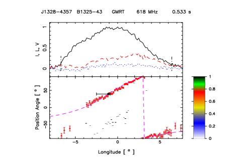
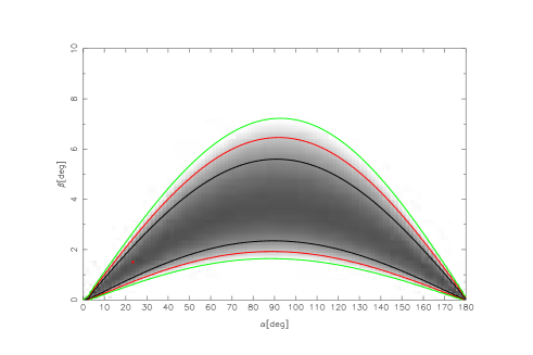
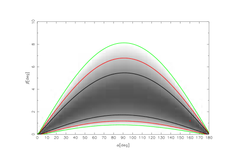
Figure 38: Top panel (upper window) shows the average profile with total intensity (Stokes I; solid black lines), total linear polarization (dashed red line) and circular polarization (Stokes V; dotted blue line). Top panel (lower window) also shows the single pulse PPA distribution (colour scale) along with the average PPA (red error bars). The RVM fits to the average PPA (dashed pink line) is also shown in this plot. Bottom panel show the $\chi^{2}$ contours for the parameters $\alpha$ and $\beta$ obtained from RVM fits.

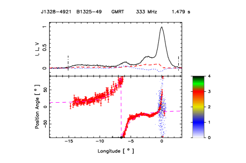
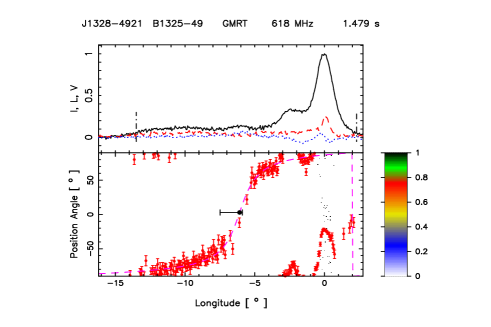
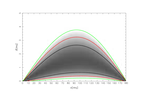
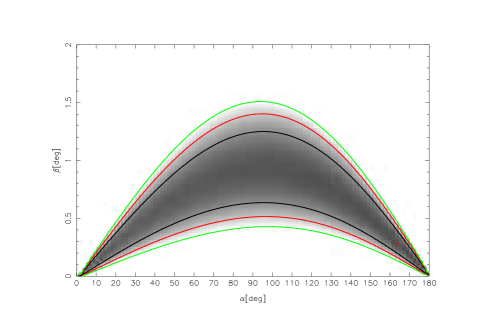
Figure 39: Top panel (upper window) shows the average profile with total intensity (Stokes I; solid black lines), total linear polarization (dashed red line) and circular polarization (Stokes V; dotted blue line). Top panel (lower window) also shows the single pulse PPA distribution (colour scale) along with the average PPA (red error bars). The RVM fits to the average PPA (dashed pink line) is also shown in this plot. Middle panel show the $\chi^{2}$ contours for the parameters $\alpha$ and $\beta$ obtained from RVM fits. Bottom panel only for 333 MHz shows the Hammer-Aitoff projection of the polarized time samples with the colour scheme representing the fractional polarization level.

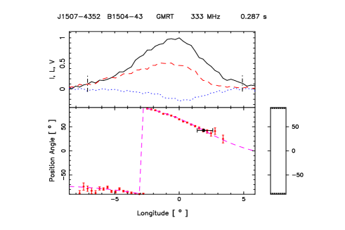
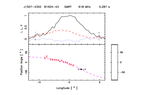
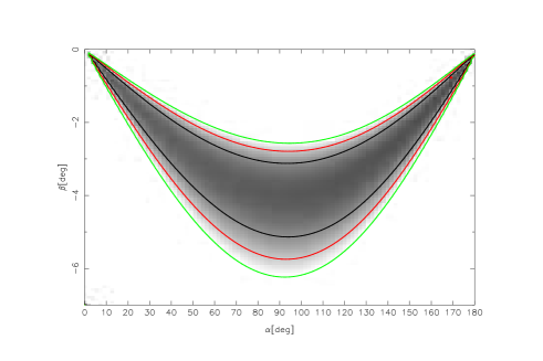
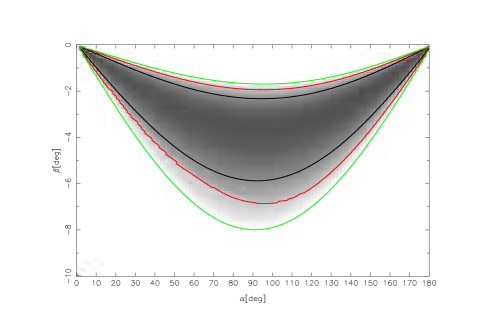
Figure 40: Top panel (upper window) shows the average profile with total intensity (Stokes I; solid black lines), total linear polarization (dashed red line) and circular polarization (Stokes V; dotted blue line). Top panel (lower window) also shows the single pulse PPA distribution (colour scale) along with the average PPA (red error bars). The RVM fits to the average PPA (dashed pink line) is also shown in this plot. Bottom panel show the $\chi^{2}$ contours for the parameters $\alpha$ and $\beta$ obtained from RVM fits.

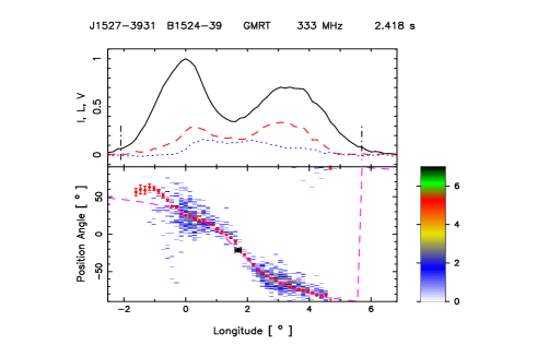
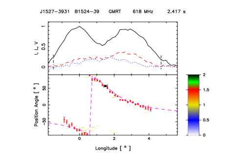
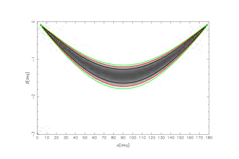
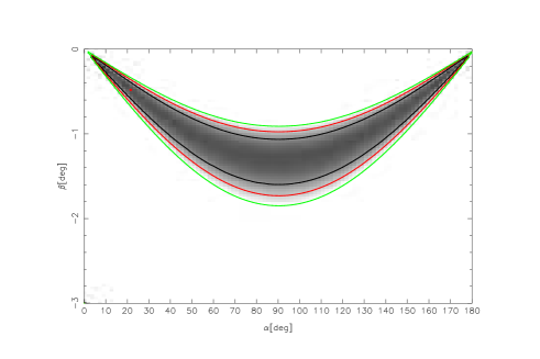
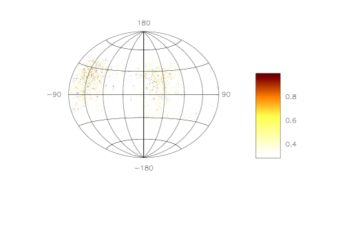
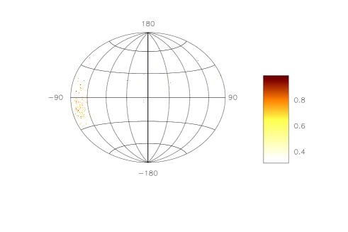
Figure 41: Top panel (upper window) shows the average profile with total intensity (Stokes I; solid black lines), total linear polarization (dashed red line) and circular polarization (Stokes V; dotted blue line). Top panel (lower window) also shows the single pulse PPA distribution (colour scale) along with the average PPA (red error bars). The RVM fits to the average PPA (dashed pink line) is also shown in this plot. Middle panel show the $\chi^{2}$ contours for the parameters $\alpha$ and $\beta$ obtained from RVM fits. Bottom panel shows the Hammer-Aitoff projection of the polarized time samples with the colour scheme representing the fractional polarization level.

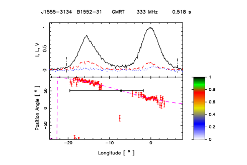
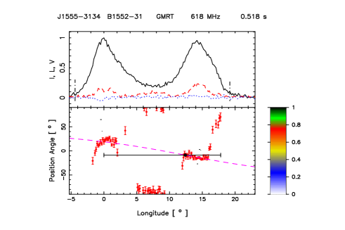
Figure 42: Top panel (upper window) shows the average profile with total intensity (Stokes I; solid black lines), total linear polarization (dashed red line) and circular polarization (Stokes V; dotted blue line). Top panel (lower window) also shows the single pulse PPA distribution (colour scale) along with the average PPA (red error bars). The RVM fits to the average PPA (dashed pink line) is also shown in this plot. Bottom panel show the $\chi^{2}$ contours for the parameters $\alpha$ and $\beta$ obtained from RVM fits.

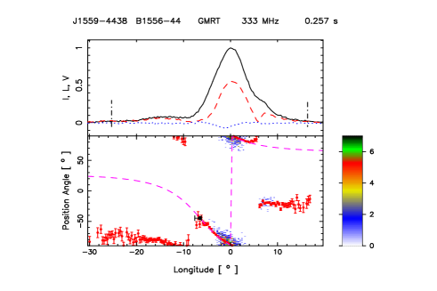
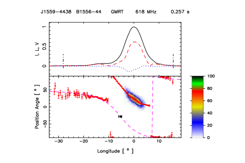
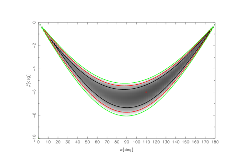
Figure 43: Top panel (upper window) shows the average profile with total intensity (Stokes I; solid black lines), total linear polarization (dashed red line) and circular polarization (Stokes V; dotted blue line). Top panel (lower window) also shows the single pulse PPA distribution (colour scale) along with the average PPA (red error bars). The RVM fits to the average PPA (dashed pink line) is also shown in this plot. Middle panel show the $\chi^{2}$ contours for the parameters $\alpha$ and $\beta$ obtained from RVM fits. Bottom panel shows the Hammer-Aitoff projection of the polarized time samples with the colour scheme representing the fractional polarization level.

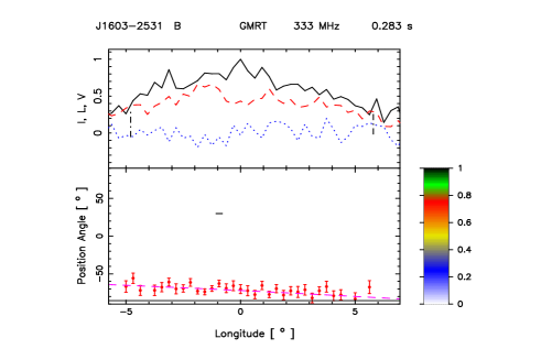
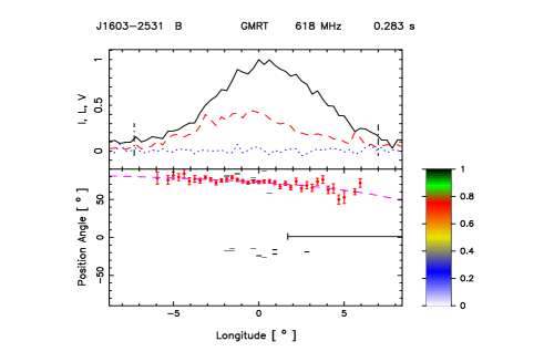
Figure 44: Top panel (upper window) shows the average profile with total intensity (Stokes I; solid black lines), total linear polarization (dashed red line) and circular polarization (Stokes V; dotted blue line). Top panel (lower window) also shows the single pulse PPA distribution (colour scale) along with the average PPA (red error bars). The RVM fits to the average PPA (dashed pink line) is also shown in this plot. Bottom panel show the $\chi^{2}$ contours for the parameters $\alpha$ and $\beta$ obtained from RVM fits.

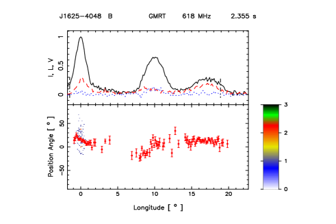
Figure 45: Top panel only for 618 MHz (upper window) shows the average profile with total intensity (Stokes I; solid black lines), total linear polarization (dashed red line) and circular polarization (Stokes V; dotted blue line). Top panel (lower window) also shows the single pulse PPA distribution (colour scale) along with the average PPA (red error bars). Bottom panel only for 618 MHz shows the Hammer-Aitoff projection of the polarized time samples with the colour scheme representing the fractional polarization level.

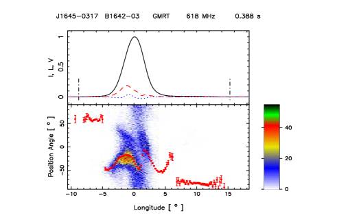
Figure 46: Top panel only for 618 MHz (upper window) shows the average profile with total intensity (Stokes I; solid black lines), total linear polarization (dashed red line) and circular polarization (Stokes V; dotted blue line). Top panel (lower window) also shows the single pulse PPA distribution (colour scale) along with the average PPA (red error bars). Bottom panel only for 618 MHz shows the Hammer-Aitoff projection of the polarized time samples with the colour scheme representing the fractional polarization level.

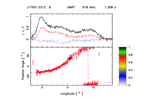
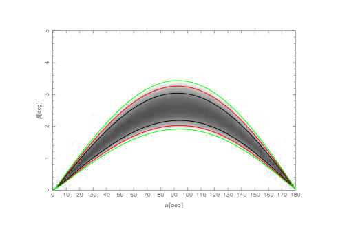
Figure 47: Top panel only for 618 MHz (upper window) shows the average profile with total intensity (Stokes I; solid black lines), total linear polarization (dashed red line) and circular polarization (Stokes V; dotted blue line). Top panel (lower window) also shows the single pulse PPA distribution (colour scale) along with the average PPA (red error bars). The RVM fits to the average PPA (dashed pink line) is also shown in this plot. Bottom panel only for 618 MHz show the $\chi^{2}$ contours for the parameters $\alpha$ and $\beta$ obtained from RVM fits.

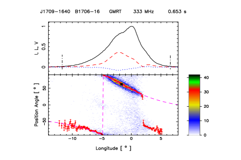
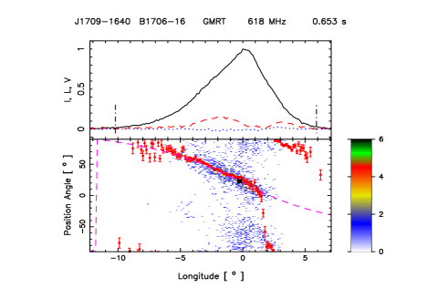
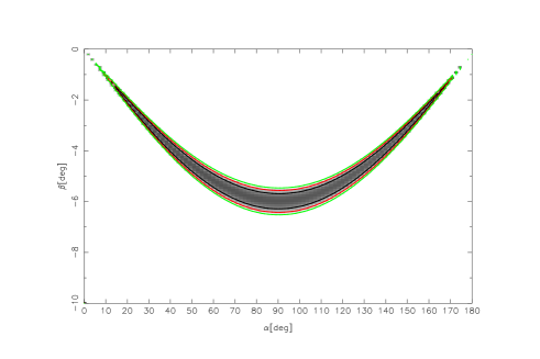
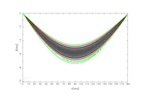
Figure 48: Top panel (upper window) shows the average profile with total intensity (Stokes I; solid black lines), total linear polarization (dashed red line) and circular polarization (Stokes V; dotted blue line). Top panel (lower window) also shows the single pulse PPA distribution (colour scale) along with the average PPA (red error bars). The RVM fits to the average PPA (dashed pink line) is also shown in this plot. Middle panel show the $\chi^{2}$ contours for the parameters $\alpha$ and $\beta$ obtained from RVM fits. Bottom panel shows the Hammer-Aitoff projection of the polarized time samples with the colour scheme representing the fractional polarization level.

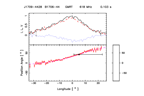
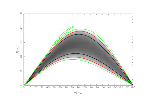
Figure 49: Top panel only for 618 MHz (upper window) shows the average profile with total intensity (Stokes I; solid black lines), total linear polarization (dashed red line) and circular polarization (Stokes V; dotted blue line). Top panel (lower window) also shows the single pulse PPA distribution (colour scale) along with the average PPA (red error bars). The RVM fits to the average PPA (dashed pink line) is also shown in this plot. Bottom panel only for 618 MHz show the $\chi^{2}$ contours for the parameters $\alpha$ and $\beta$ obtained from RVM fits.

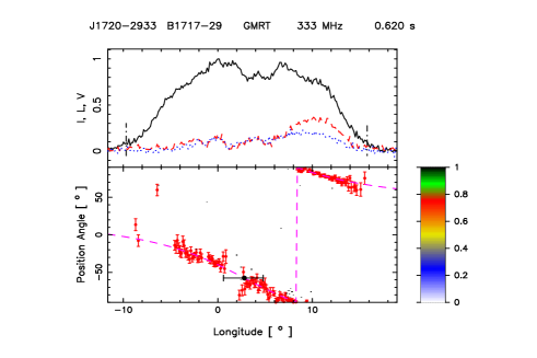
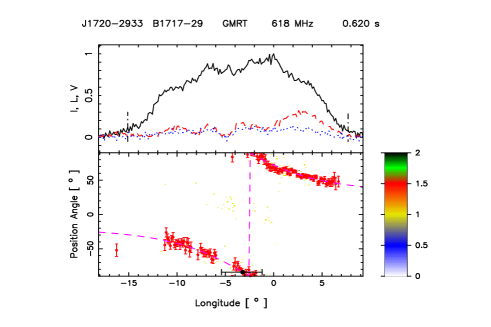
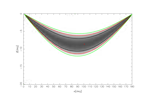
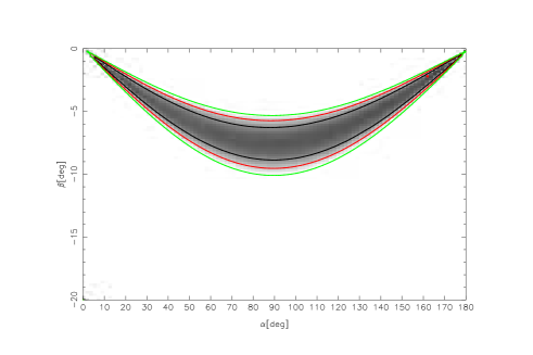
Figure 50: Top panel (upper window) shows the average profile with total intensity (Stokes I; solid black lines), total linear polarization (dashed red line) and circular polarization (Stokes V; dotted blue line). Top panel (lower window) also shows the single pulse PPA distribution (colour scale) along with the average PPA (red error bars). The RVM fits to the average PPA (dashed pink line) is also shown in this plot. Middle panel show the $\chi^{2}$ contours for the parameters $\alpha$ and $\beta$ obtained from RVM fits. Bottom panel only for 618 MHz shows the Hammer-Aitoff projection of the polarized time samples with the colour scheme representing the fractional polarization level.

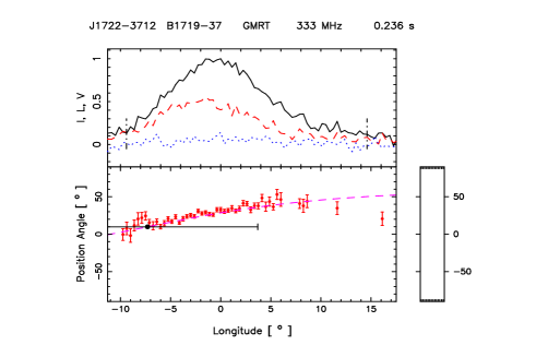
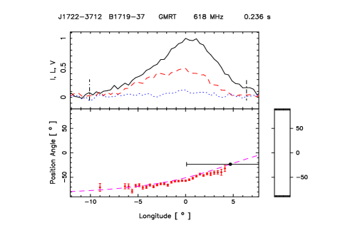
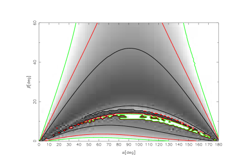
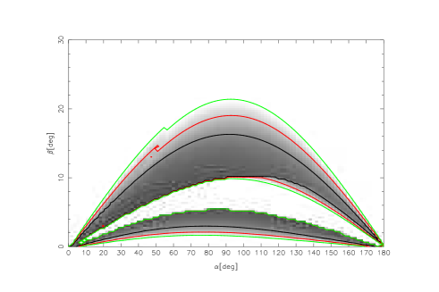
Figure 51: Top panel (upper window) shows the average profile with total intensity (Stokes I; solid black lines), total linear polarization (dashed red line) and circular polarization (Stokes V; dotted blue line). Top panel (lower window) also shows the single pulse PPA distribution (colour scale) along with the average PPA (red error bars). The RVM fits to the average PPA (dashed pink line) is also shown in this plot. Bottom panel show the $\chi^{2}$ contours for the parameters $\alpha$ and $\beta$ obtained from RVM fits.

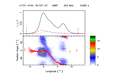
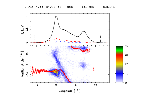
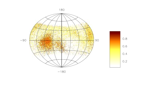
Figure 52: Top panel (upper window) shows the average profile with total intensity (Stokes I; solid black lines), total linear polarization (dashed red line) and circular polarization (Stokes V; dotted blue line). Top panel (lower window) also shows the single pulse PPA distribution (colour scale) along with the average PPA (red error bars). Bottom panel shows the Hammer-Aitoff projection of the polarized time samples with the colour scheme representing the fractional polarization level.

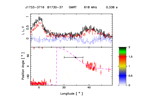
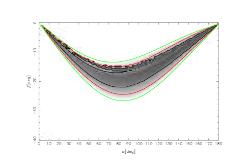
Figure 53: Top panel only for 618 MHz (upper window) shows the average profile with total intensity (Stokes I; solid black lines), total linear polarization (dashed red line) and circular polarization (Stokes V; dotted blue line). Top panel (lower window) also shows the single pulse PPA distribution (colour scale) along with the average PPA (red error bars). The RVM fits to the average PPA (dashed pink line) is also shown in this plot. Middle panel only for 618 MHz show the $\chi^{2}$ contours for the parameters $\alpha$ and $\beta$ obtained from RVM fits. Bottom panel only for 618 MHz shows the Hammer-Aitoff projection of the polarized time samples with the colour scheme representing the fractional polarization level.

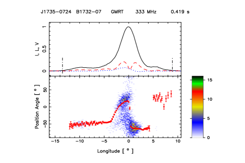
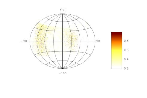
Figure 54: Top panel only for 333 MHz (upper window) shows the average profile with total intensity (Stokes I; solid black lines), total linear polarization (dashed red line) and circular polarization (Stokes V; dotted blue line). Top panel (lower window) also shows the single pulse PPA distribution (colour scale) along with the average PPA (red error bars). Bottom panel only for 333 MHz shows the Hammer-Aitoff projection of the polarized time samples with the colour scheme representing the fractional polarization level.

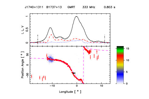
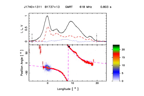
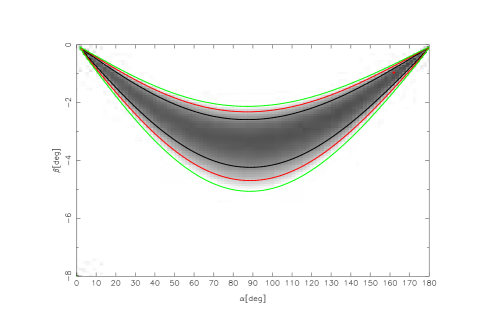
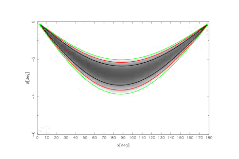
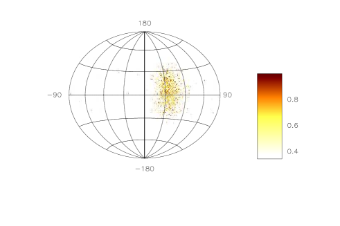
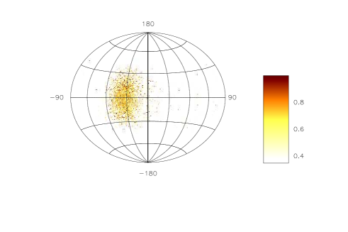
Figure 55: Top panel (upper window) shows the average profile with total intensity (Stokes I; solid black lines), total linear polarization (dashed red line) and circular polarization (Stokes V; dotted blue line). Top panel (lower window) also shows the single pulse PPA distribution (colour scale) along with the average PPA (red error bars). The RVM fits to the average PPA (dashed pink line) is also shown in this plot. Middle panel show the $\chi^{2}$ contours for the parameters $\alpha$ and $\beta$ obtained from RVM fits. Bottom panel shows the Hammer-Aitoff projection of the polarized time samples with the colour scheme representing the fractional polarization level.

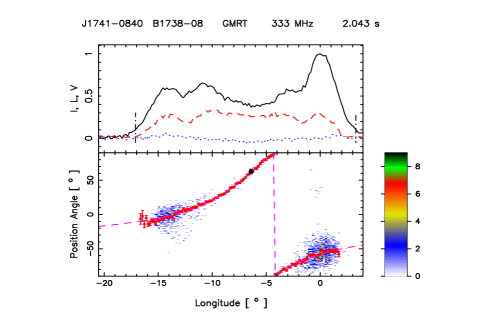
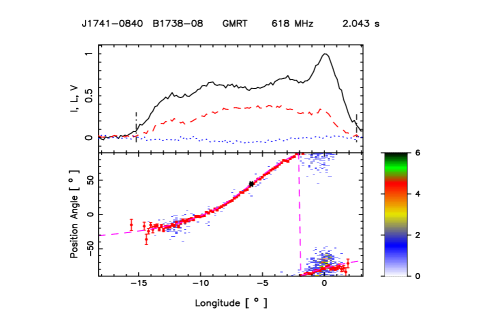
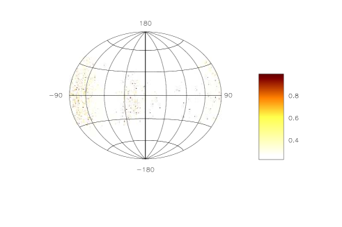
Figure 56: Top panel (upper window) shows the average profile with total intensity (Stokes I; solid black lines), total linear polarization (dashed red line) and circular polarization (Stokes V; dotted blue line). Top panel (lower window) also shows the single pulse PPA distribution (colour scale) along with the average PPA (red error bars). The RVM fits to the average PPA (dashed pink line) is also shown in this plot. Middle panel show the $\chi^{2}$ contours for the parameters $\alpha$ and $\beta$ obtained from RVM fits. Bottom panel shows the Hammer-Aitoff projection of the polarized time samples with the colour scheme representing the fractional polarization level.

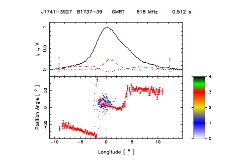
Figure 57: Top panel only for 618 MHz (upper window) shows the average profile with total intensity (Stokes I; solid black lines), total linear polarization (dashed red line) and circular polarization (Stokes V; dotted blue line). Top panel (lower window) also shows the single pulse PPA distribution (colour scale) along with the average PPA (red error bars). The RVM fits to the average PPA (dashed pink line) is also shown in this plot. Middle panel only for 618 MHz show the $\chi^{2}$ contours for the parameters $\alpha$ and $\beta$ obtained from RVM fits. Bottom panel only for 618 MHz shows the Hammer-Aitoff projection of the polarized time samples with the colour scheme representing the fractional polarization level.

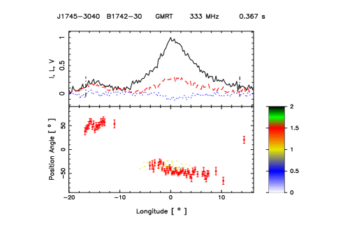
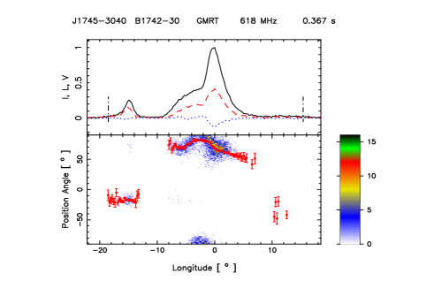
Figure 58: Top panel (upper window) shows the average profile with total intensity (Stokes I; solid black lines), total linear polarization (dashed red line) and circular polarization (Stokes V; dotted blue line). Top panel (lower window) also shows the single pulse PPA distribution (colour scale) along with the average PPA (red error bars). Bottom panel shows the Hammer-Aitoff projection of the polarized time samples with the colour scheme representing the fractional polarization level.

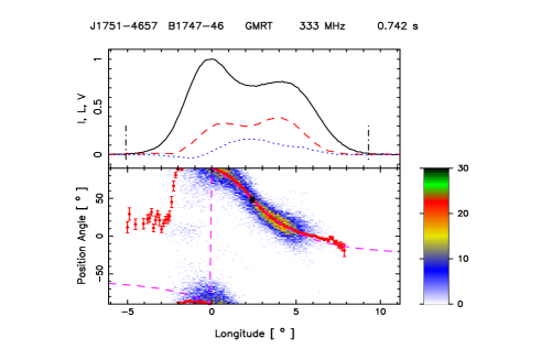
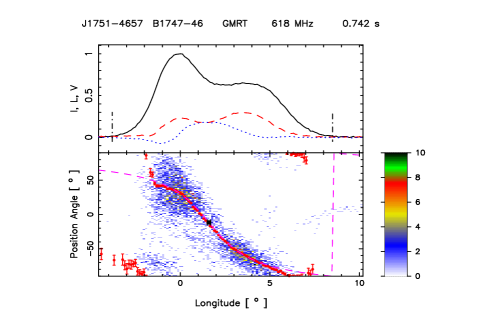
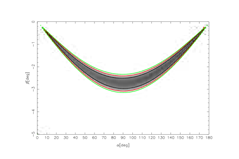
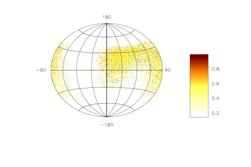
Figure 59: Top panel (upper window) shows the average profile with total intensity (Stokes I; solid black lines), total linear polarization (dashed red line) and circular polarization (Stokes V; dotted blue line). Top panel (lower window) also shows the single pulse PPA distribution (colour scale) along with the average PPA (red error bars). The RVM fits to the average PPA (dashed pink line) is also shown in this plot. Middle panel show the $\chi^{2}$ contours for the parameters $\alpha$ and $\beta$ obtained from RVM fits. Bottom panel shows the Hammer-Aitoff projection of the polarized time samples with the colour scheme representing the fractional polarization level.

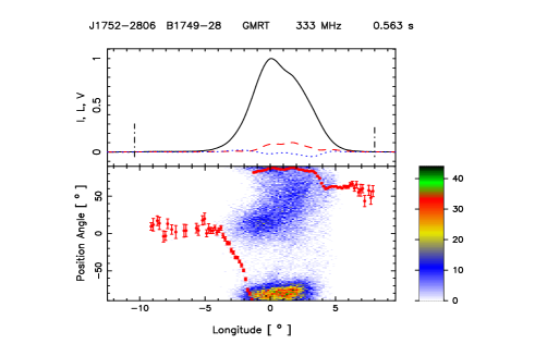
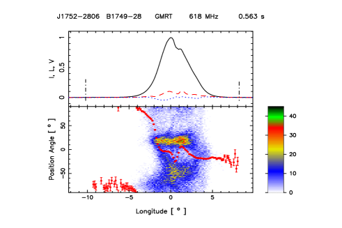
Figure 60: Top panel (upper window) shows the average profile with total intensity (Stokes I; solid black lines), total linear polarization (dashed red line) and circular polarization (Stokes V; dotted blue line). Top panel (lower window) also shows the single pulse PPA distribution (colour scale) along with the average PPA (red error bars). Bottom panel shows the Hammer-Aitoff projection of the polarized time samples with the colour scheme representing the fractional polarization level.

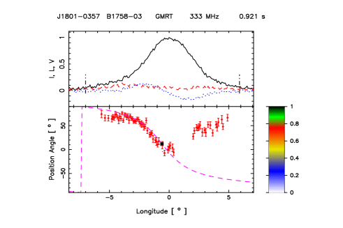
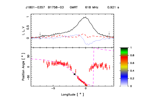
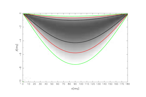
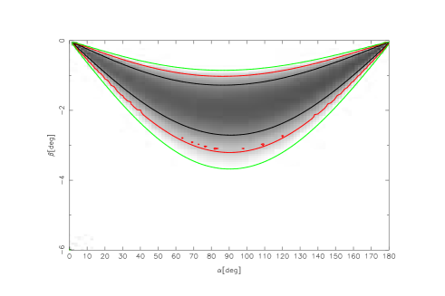
Figure 61: Top panel (upper window) shows the average profile with total intensity (Stokes I; solid black lines), total linear polarization (dashed red line) and circular polarization (Stokes V; dotted blue line). Top panel (lower window) also shows the single pulse PPA distribution (colour scale) along with the average PPA (red error bars). The RVM fits to the average PPA (dashed pink line) is also shown in this plot. Bottom panel show the $\chi^{2}$ contours for the parameters $\alpha$ and $\beta$ obtained from RVM fits.

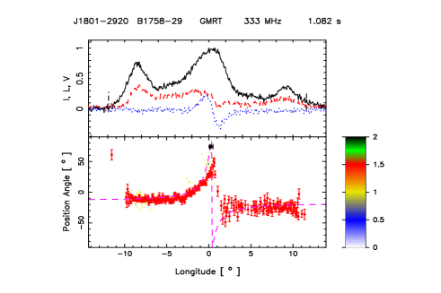
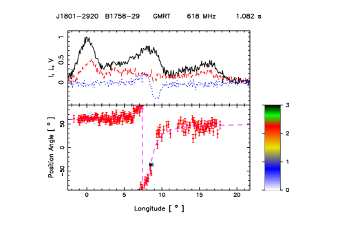
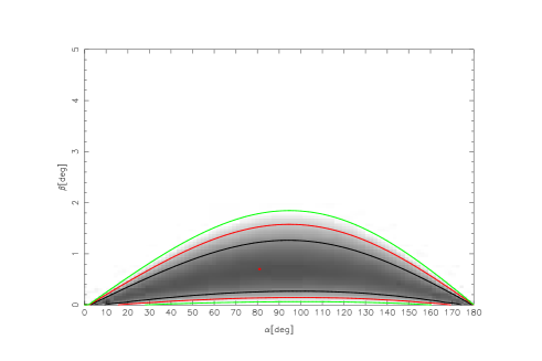
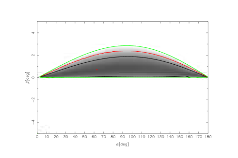
Figure 62: Top panel (upper window) shows the average profile with total intensity (Stokes I; solid black lines), total linear polarization (dashed red line) and circular polarization (Stokes V; dotted blue line). Top panel (lower window) also shows the single pulse PPA distribution (colour scale) along with the average PPA (red error bars). The RVM fits to the average PPA (dashed pink line) is also shown in this plot. Middle panel show the $\chi^{2}$ contours for the parameters $\alpha$ and $\beta$ obtained from RVM fits. Bottom panel only for 333 MHz shows the Hammer-Aitoff projection of the polarized time samples with the colour scheme representing the fractional polarization level.

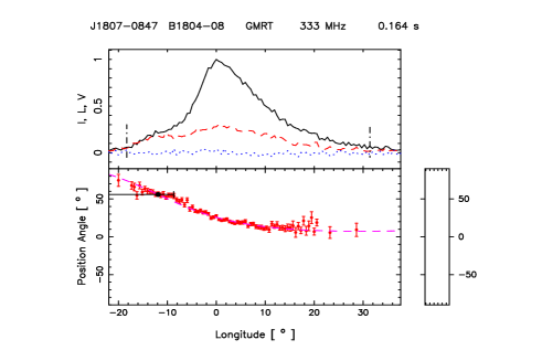
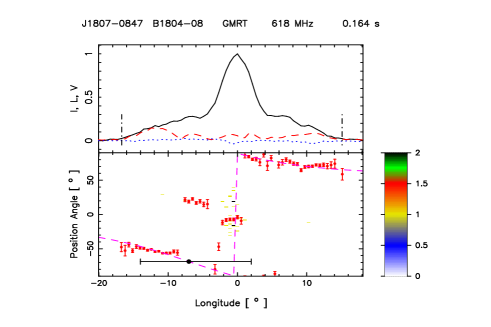
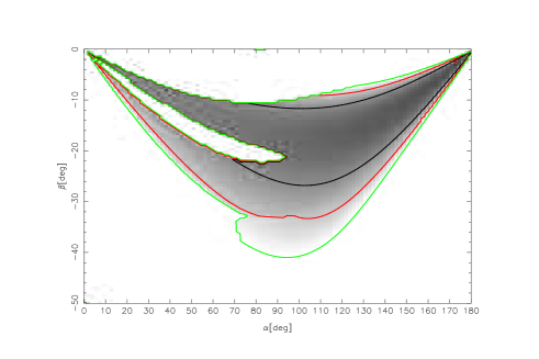
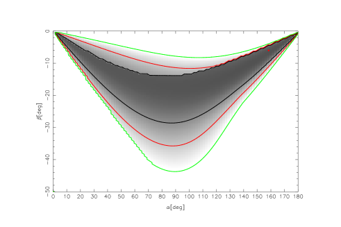
Figure 63: Top panel (upper window) shows the average profile with total intensity (Stokes I; solid black lines), total linear polarization (dashed red line) and circular polarization (Stokes V; dotted blue line). Top panel (lower window) also shows the single pulse PPA distribution (colour scale) along with the average PPA (red error bars). The RVM fits to the average PPA (dashed pink line) is also shown in this plot. Bottom panel show the $\chi^{2}$ contours for the parameters $\alpha$ and $\beta$ obtained from RVM fits.

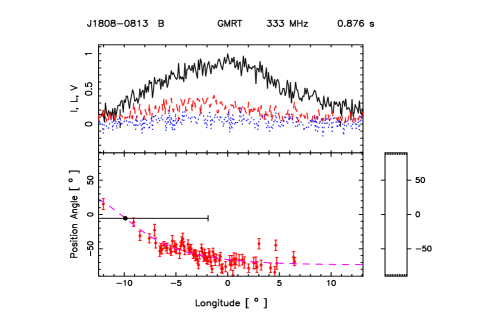
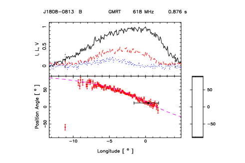
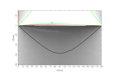
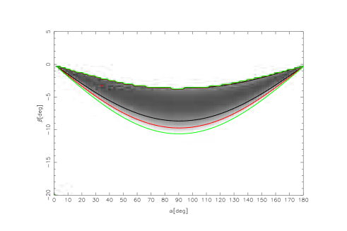
Figure 64: Top panel (upper window) shows the average profile with total intensity (Stokes I; solid black lines), total linear polarization (dashed red line) and circular polarization (Stokes V; dotted blue line). Top panel (lower window) also shows the single pulse PPA distribution (colour scale) along with the average PPA (red error bars). The RVM fits to the average PPA (dashed pink line) is also shown in this plot. Bottom panel show the $\chi^{2}$ contours for the parameters $\alpha$ and $\beta$ obtained from RVM fits.

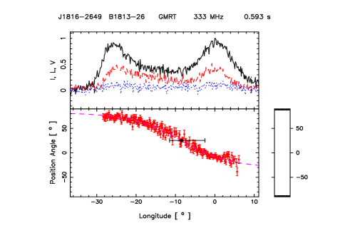
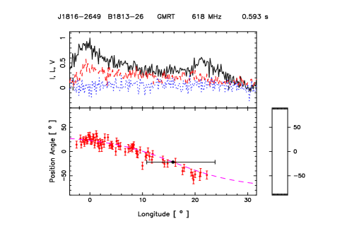
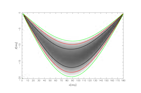
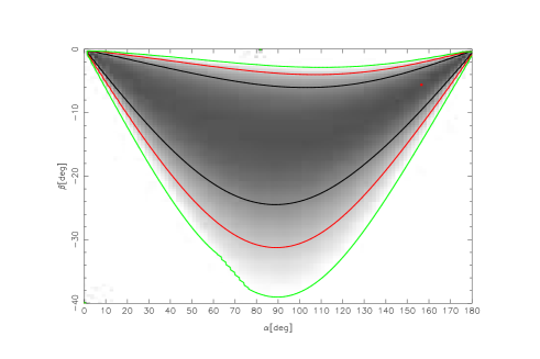
Figure 65: Top panel (upper window) shows the average profile with total intensity (Stokes I; solid black lines), total linear polarization (dashed red line) and circular polarization (Stokes V; dotted blue line). Top panel (lower window) also shows the single pulse PPA distribution (colour scale) along with the average PPA (red error bars). The RVM fits to the average PPA (dashed pink line) is also shown in this plot. Bottom panel show the $\chi^{2}$ contours for the parameters $\alpha$ and $\beta$ obtained from RVM fits.

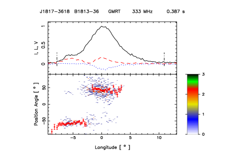
Figure 66: Top panel (upper window) shows the average profile with total intensity (Stokes I; solid black lines), total linear polarization (dashed red line) and circular polarization (Stokes V; dotted blue line). Top panel (lower window) also shows the single pulse PPA distribution (colour scale) along with the average PPA (red error bars). The RVM fits to the average PPA (dashed pink line) is also shown in this plot. Bottom panel show the $\chi^{2}$ contours for the parameters $\alpha$ and $\beta$ obtained from RVM fits.

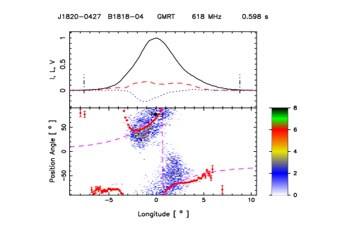
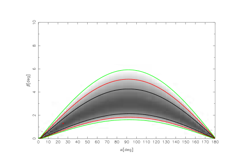
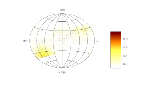
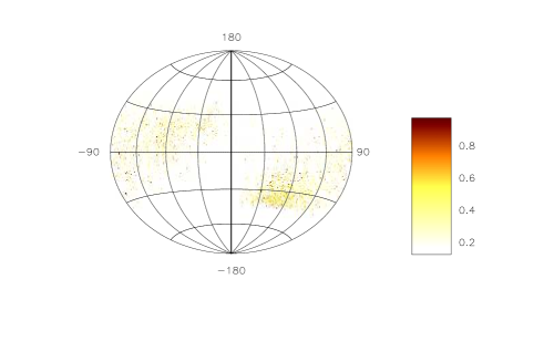
Figure 67: Top panel (upper window) shows the average profile with total intensity (Stokes I; solid black lines), total linear polarization (dashed red line) and circular polarization (Stokes V; dotted blue line). Top panel (lower window) also shows the single pulse PPA distribution (colour scale) along with the average PPA (red error bars). The RVM fits to the average PPA (dashed pink line) is also shown in this plot. Middle panel only for 618 MHz show the $\chi^{2}$ contours for the parameters $\alpha$ and $\beta$ obtained from RVM fits. Bottom panel shows the Hammer-Aitoff projection of the polarized time samples with the colour scheme representing the fractional polarization level.

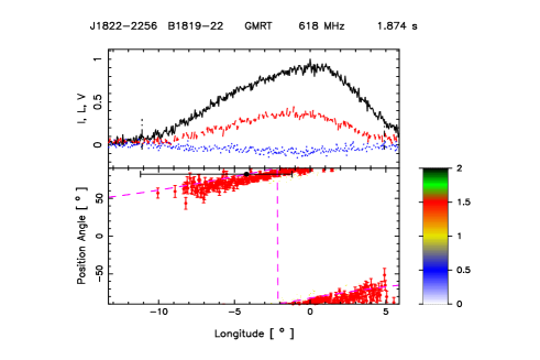
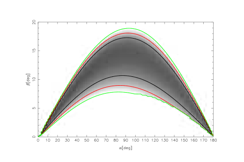
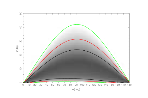
Figure 68: Top panel (upper window) shows the average profile with total intensity (Stokes I; solid black lines), total linear polarization (dashed red line) and circular polarization (Stokes V; dotted blue line). Top panel (lower window) also shows the single pulse PPA distribution (colour scale) along with the average PPA (red error bars). The RVM fits to the average PPA (dashed pink line) is also shown in this plot. Middle panel show the $\chi^{2}$ contours for the parameters $\alpha$ and $\beta$ obtained from RVM fits. Bottom panel only for 618 MHz shows the Hammer-Aitoff projection of the polarized time samples with the colour scheme representing the fractional polarization level.

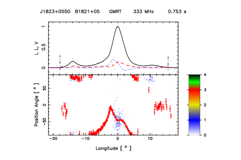
Figure 69: Top panel only for 333 MHz (upper window) shows the average profile with total intensity (Stokes I; solid black lines), total linear polarization (dashed red line) and circular polarization (Stokes V; dotted blue line). Top panel (lower window) also shows the single pulse PPA distribution (colour scale) along with the average PPA (red error bars). Bottom panel only for 333 MHz shows the Hammer-Aitoff projection of the polarized time samples with the colour scheme representing the fractional polarization level.

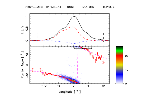
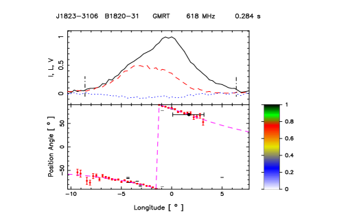
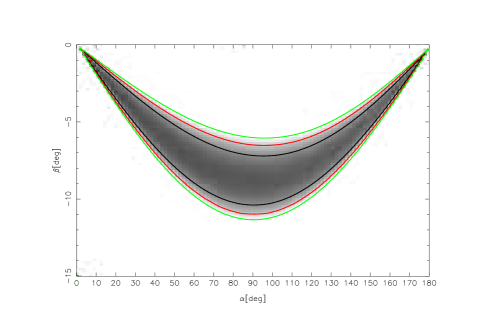
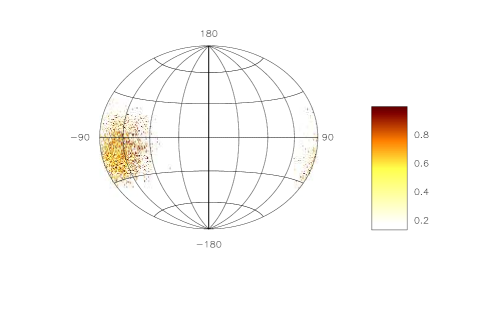
Figure 70: Top panel (upper window) shows the average profile with total intensity (Stokes I; solid black lines), total linear polarization (dashed red line) and circular polarization (Stokes V; dotted blue line). Top panel (lower window) also shows the single pulse PPA distribution (colour scale) along with the average PPA (red error bars). The RVM fits to the average PPA (dashed pink line) is also shown in this plot. Middle panel show the $\chi^{2}$ contours for the parameters $\alpha$ and $\beta$ obtained from RVM fits. Bottom panel only for 333 MHz shows the Hammer-Aitoff projection of the polarized time samples with the colour scheme representing the fractional polarization level.

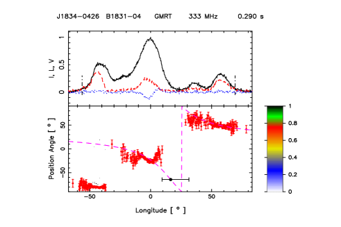
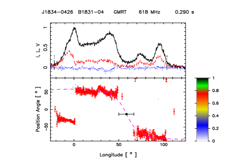
Figure 71: Top panel (upper window) shows the average profile with total intensity (Stokes I; solid black lines), total linear polarization (dashed red line) and circular polarization (Stokes V; dotted blue line). Top panel (lower window) also shows the single pulse PPA distribution (colour scale) along with the average PPA (red error bars). The RVM fits to the average PPA (dashed pink line) is also shown in this plot. Bottom panel show the $\chi^{2}$ contours for the parameters $\alpha$ and $\beta$ obtained from RVM fits.

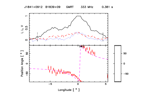
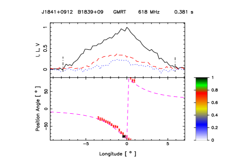
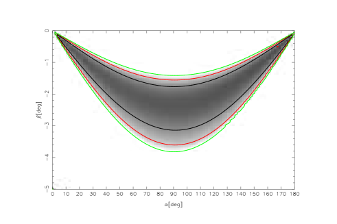
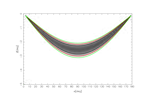
Figure 72: Top panel (upper window) shows the average profile with total intensity (Stokes I; solid black lines), total linear polarization (dashed red line) and circular polarization (Stokes V; dotted blue line). Top panel (lower window) also shows the single pulse PPA distribution (colour scale) along with the average PPA (red error bars). The RVM fits to the average PPA (dashed pink line) is also shown in this plot. Bottom panel show the $\chi^{2}$ contours for the parameters $\alpha$ and $\beta$ obtained from RVM fits.

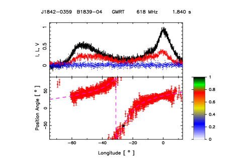
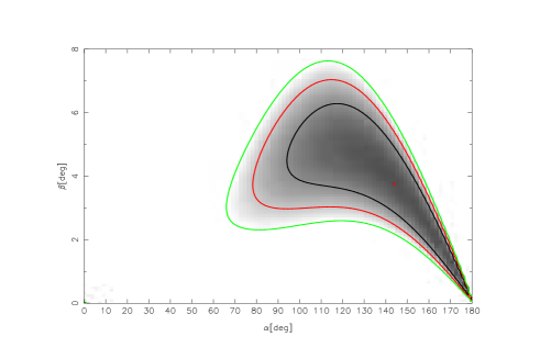
Figure 73: Top panel only for 618 MHz (upper window) shows the average profile with total intensity (Stokes I; solid black lines), total linear polarization (dashed red line) and circular polarization (Stokes V; dotted blue line). Top panel (lower window) also shows the single pulse PPA distribution (colour scale) along with the average PPA (red error bars). The RVM fits to the average PPA (dashed pink line) is also shown in this plot. Bottom panel only for 618 MHz show the $\chi^{2}$ contours for the parameters $\alpha$ and $\beta$ obtained from RVM fits.

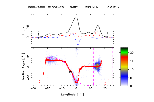
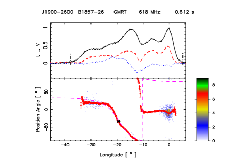
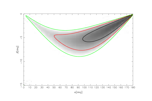
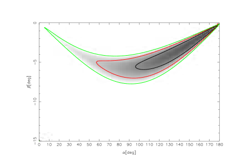
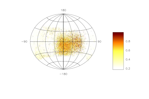
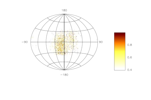
Figure 74: Top panel (upper window) shows the average profile with total intensity (Stokes I; solid black lines), total linear polarization (dashed red line) and circular polarization (Stokes V; dotted blue line). Top panel (lower window) also shows the single pulse PPA distribution (colour scale) along with the average PPA (red error bars). The RVM fits to the average PPA (dashed pink line) is also shown in this plot. Middle panel show the $\chi^{2}$ contours for the parameters $\alpha$ and $\beta$ obtained from RVM fits. Bottom panel shows the Hammer-Aitoff projection of the polarized time samples with the colour scheme representing the fractional polarization level.

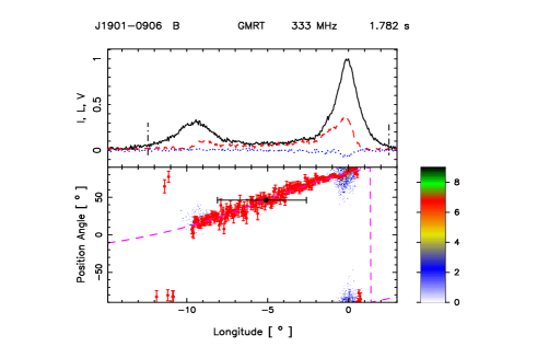
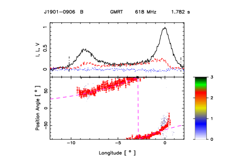
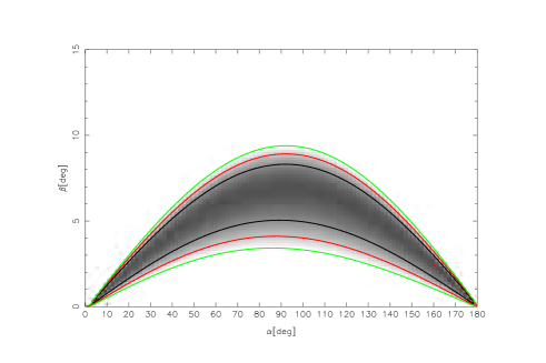
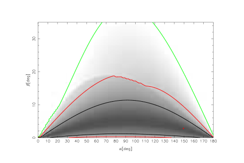
Figure 75: Top panel (upper window) shows the average profile with total intensity (Stokes I; solid black lines), total linear polarization (dashed red line) and circular polarization (Stokes V; dotted blue line). Top panel (lower window) also shows the single pulse PPA distribution (colour scale) along with the average PPA (red error bars). The RVM fits to the average PPA (dashed pink line) is also shown in this plot. Middle panel show the $\chi^{2}$ contours for the parameters $\alpha$ and $\beta$ obtained from RVM fits. Bottom panel shows the Hammer-Aitoff projection of the polarized time samples with the colour scheme representing the fractional polarization level.

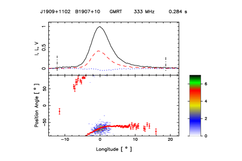
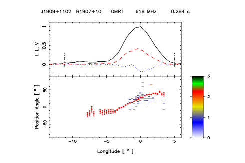
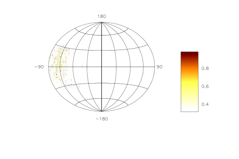
Figure 76: Top panel (upper window) shows the average profile with total intensity (Stokes I; solid black lines), total linear polarization (dashed red line) and circular polarization (Stokes V; dotted blue line). Top panel (lower window) also shows the single pulse PPA distribution (colour scale) along with the average PPA (red error bars). Bottom panel shows the Hammer-Aitoff projection of the polarized time samples with the colour scheme representing the fractional polarization level.

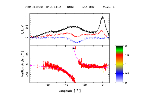
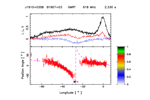
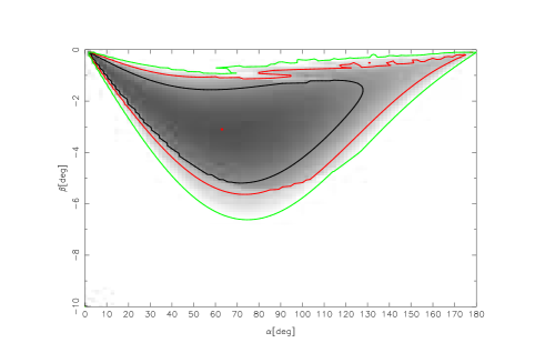
Figure 77: Top panel (upper window) shows the average profile with total intensity (Stokes I; solid black lines), total linear polarization (dashed red line) and circular polarization (Stokes V; dotted blue line). Top panel (lower window) also shows the single pulse PPA distribution (colour scale) along with the average PPA (red error bars). The RVM fits to the average PPA (dashed pink line) is also shown in this plot. Bottom panel show the $\chi^{2}$ contours for the parameters $\alpha$ and $\beta$ obtained from RVM fits.

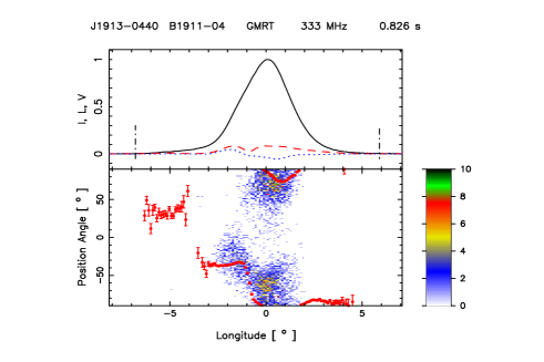
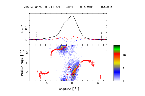
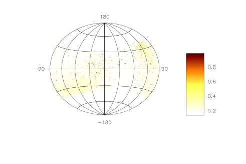
Figure 78: Top panel (upper window) shows the average profile with total intensity (Stokes I; solid black lines), total linear polarization (dashed red line) and circular polarization (Stokes V; dotted blue line). Top panel (lower window) also shows the single pulse PPA distribution (colour scale) along with the average PPA (red error bars). Bottom panel shows the Hammer-Aitoff projection of the polarized time samples with the colour scheme representing the fractional polarization level.

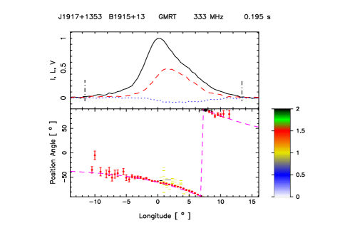
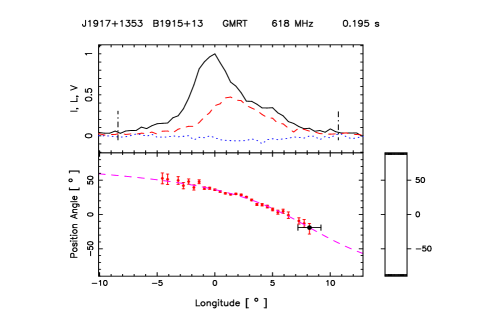
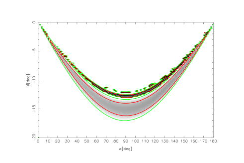
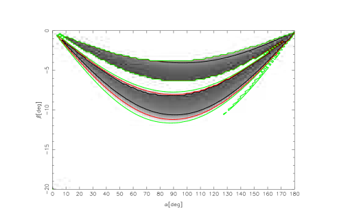
Figure 79: Top panel (upper window) shows the average profile with total intensity (Stokes I; solid black lines), total linear polarization (dashed red line) and circular polarization (Stokes V; dotted blue line). Top panel (lower window) also shows the single pulse PPA distribution (colour scale) along with the average PPA (red error bars). The RVM fits to the average PPA (dashed pink line) is also shown in this plot. Bottom panel show the $\chi^{2}$ contours for the parameters $\alpha$ and $\beta$ obtained from RVM fits.

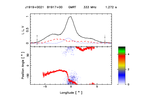
Figure 80: Top panel only for 333 MHz (upper window) shows the average profile with total intensity (Stokes I; solid black lines), total linear polarization (dashed red line) and circular polarization (Stokes V; dotted blue line). Top panel (lower window) also shows the single pulse PPA distribution (colour scale) along with the average PPA (red error bars). Bottom panel only for 333 MHz shows the Hammer-Aitoff projection of the polarized time samples with the colour scheme representing the fractional polarization level.

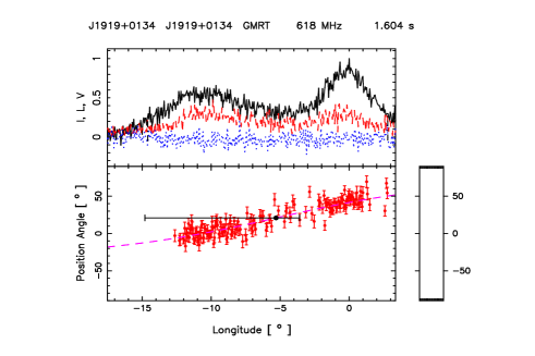
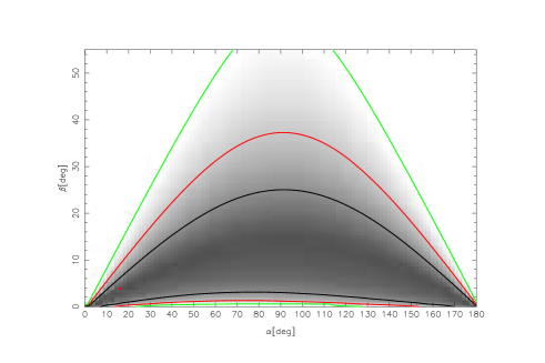
Figure 81: Top panel only for 618 MHz (upper window) shows the average profile with total intensity (Stokes I; solid black lines), total linear polarization (dashed red line) and circular polarization (Stokes V; dotted blue line). Top panel (lower window) also shows the single pulse PPA distribution (colour scale) along with the average PPA (red error bars). The RVM fits to the average PPA (dashed pink line) is also shown in this plot. Bottom panel only at 618 MHz show the $\chi^{2}$ contours for the parameters $\alpha$ and $\beta$ obtained from RVM fits.

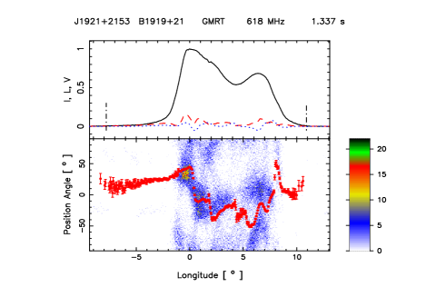
Figure 82: Top panel only at 618 MHz (upper window) shows the average profile with total intensity (Stokes I; solid black lines), total linear polarization (dashed red line) and circular polarization (Stokes V; dotted blue line). Top panel (lower window) also shows the single pulse PPA distribution (colour scale) along with the average PPA (red error bars). Bottom panel only at 618 MHz shows the Hammer-Aitoff projection of the polarized time samples with the colour scheme representing the fractional polarization level.

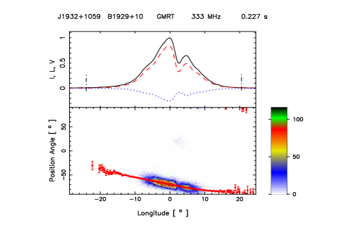
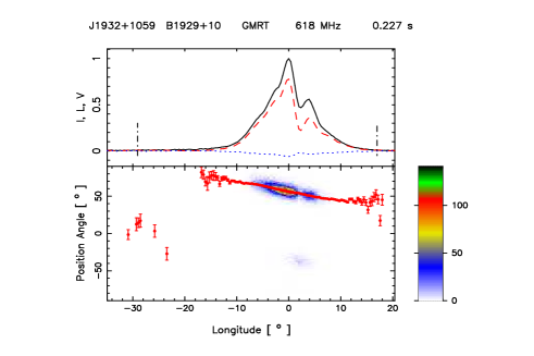
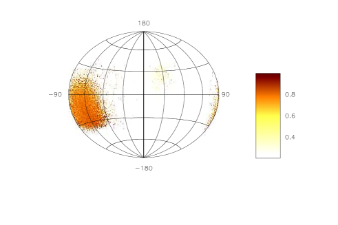
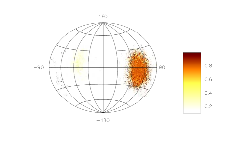
Figure 83: Top panel (upper window) shows the average profile with total intensity (Stokes I; solid black lines), total linear polarization (dashed red line) and circular polarization (Stokes V; dotted blue line). Top panel (lower window) also shows the single pulse PPA distribution (colour scale) along with the average PPA (red error bars). Bottom panel shows the Hammer-Aitoff projection of the polarized time samples with the colour scheme representing the fractional polarization level.

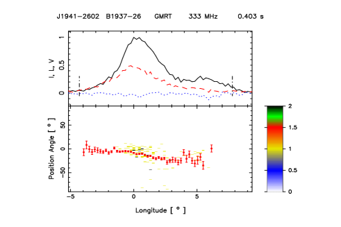
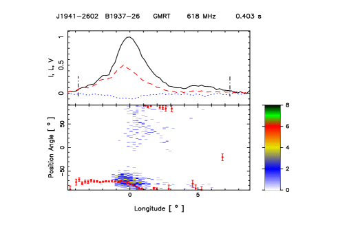
Figure 84: Top panel (upper window) shows the average profile with total intensity (Stokes I; solid black lines), total linear polarization (dashed red line) and circular polarization (Stokes V; dotted blue line). Top panel (lower window) also shows the single pulse PPA distribution (colour scale) along with the average PPA (red error bars). Bottom panel shows the Hammer-Aitoff projection of the polarized time samples with the colour scheme representing the fractional polarization level.

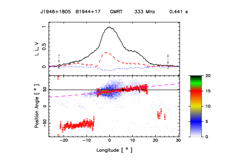
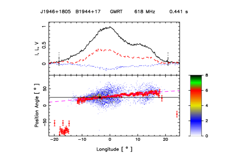
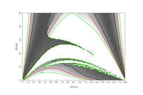
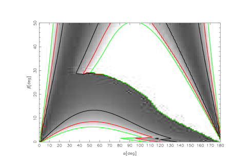
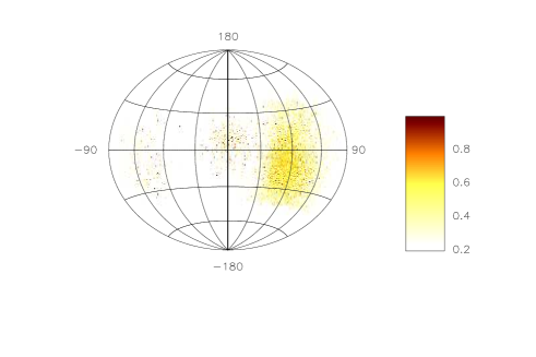
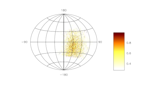
Figure 85: Top panel (upper window) shows the average profile with total intensity (Stokes I; solid black lines), total linear polarization (dashed red line) and circular polarization (Stokes V; dotted blue line). Top panel (lower window) also shows the single pulse PPA distribution (colour scale) along with the average PPA (red error bars). The RVM fits to the average PPA (dashed pink line) is also shown in this plot. Middle panel show the $\chi^{2}$ contours for the parameters $\alpha$ and $\beta$ obtained from RVM fits. Bottom panel shows the Hammer-Aitoff projection of the polarized time samples with the colour scheme representing the fractional polarization level.

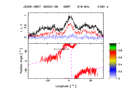
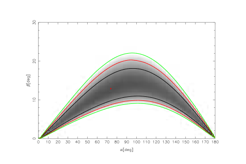
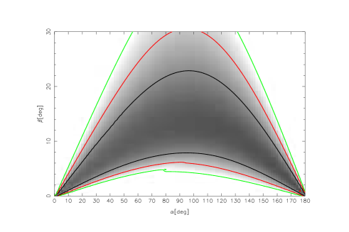
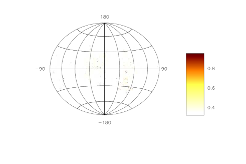
Figure 86: Top panel (upper window) shows the average profile with total intensity (Stokes I; solid black lines), total linear polarization (dashed red line) and circular polarization (Stokes V; dotted blue line). Top panel (lower window) also shows the single pulse PPA distribution (colour scale) along with the average PPA (red error bars). The RVM fits to the average PPA (dashed pink line) is also shown in this plot. Middle panel show the $\chi^{2}$ contours for the parameters $\alpha$ and $\beta$ obtained from RVM fits. Bottom panel only for 333 MHz shows the Hammer-Aitoff projection of the polarized time samples with the colour scheme representing the fractional polarization level.

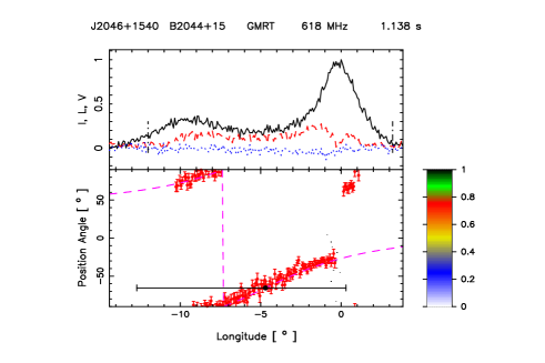
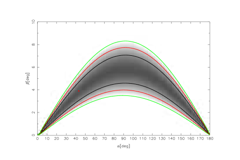
Figure 87: Top panel only at 618 MHz (upper window) shows the average profile with total intensity (Stokes I; solid black lines), total linear polarization (dashed red line) and circular polarization (Stokes V; dotted blue line). Top panel (lower window) also shows the single pulse PPA distribution (colour scale) along with the average PPA (red error bars). The RVM fits to the average PPA (dashed pink line) is also shown in this plot. Bottom panel only at 618 MHz show the $\chi^{2}$ contours for the parameters $\alpha$ and $\beta$ obtained from RVM fits.

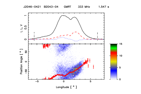
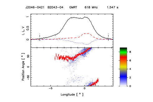
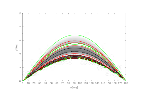
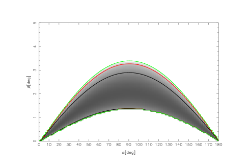
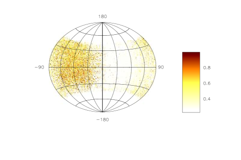
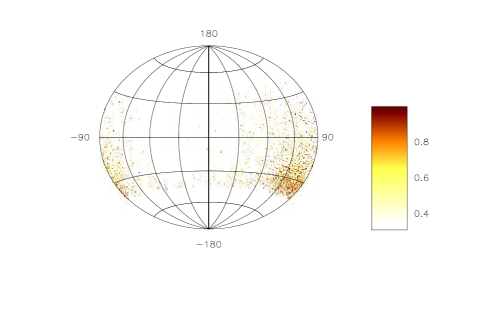
Figure 88: Top panel (upper window) shows the average profile with total intensity (Stokes I; solid black lines), total linear polarization (dashed red line) and circular polarization (Stokes V; dotted blue line). Top panel (lower window) also shows the single pulse PPA distribution (colour scale) along with the average PPA (red error bars). The RVM fits to the average PPA (dashed pink line) is also shown in this plot. Middle panel show the $\chi^{2}$ contours for the parameters $\alpha$ and $\beta$ obtained from RVM fits. Bottom panel shows the Hammer-Aitoff projection of the polarized time samples with the colour scheme representing the fractional polarization level.

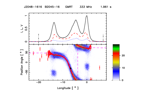
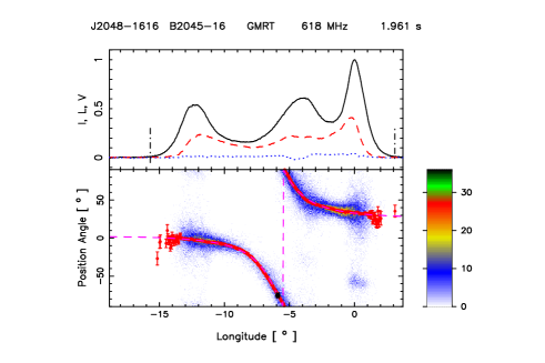
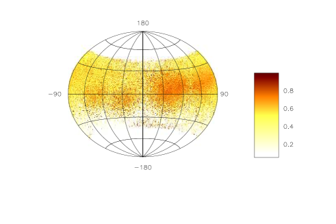
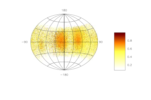
Figure 89: Top panel (upper window) shows the average profile with total intensity (Stokes I; solid black lines), total linear polarization (dashed red line) and circular polarization (Stokes V; dotted blue line). Top panel (lower window) also shows the single pulse PPA distribution (colour scale) along with the average PPA (red error bars). The RVM fits to the average PPA (dashed pink line) is also shown in this plot. Middle panel show the $\chi^{2}$ contours for the parameters $\alpha$ and $\beta$ obtained from RVM fits. Bottom panel shows the Hammer-Aitoff projection of the polarized time samples with the colour scheme representing the fractional polarization level.

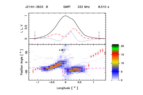
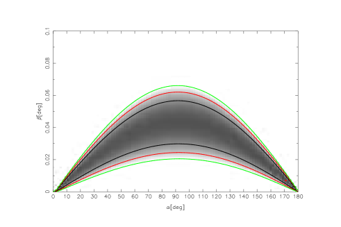
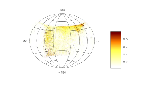
Figure 90: Top panel only at 618 MHz (upper window) shows the average profile with total intensity (Stokes I; solid black lines), total linear polarization (dashed red line) and circular polarization (Stokes V; dotted blue line). Top panel (lower window) also shows the single pulse PPA distribution (colour scale) along with the average PPA (red error bars). The RVM fits to the average PPA (dashed pink line) is also shown in this plot. Middle panel only at 618 MHz show the $\chi^{2}$ contours for the parameters $\alpha$ and $\beta$ obtained from RVM fits. Bottom panel only at 618 MHz shows the Hammer-Aitoff projection of the polarized time samples with the colour scheme representing the fractional polarization level.

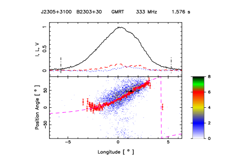
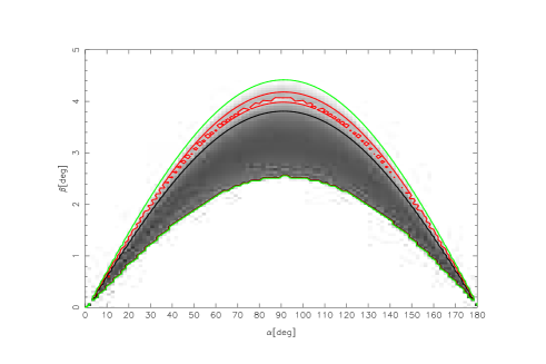
Figure 91: Top panel only at 333 MHz (upper window) shows the average profile with total intensity (Stokes I; solid black lines), total linear polarization (dashed red line) and circular polarization (Stokes V; dotted blue line). Top panel (lower window) also shows the single pulse PPA distribution (colour scale) along with the average PPA (red error bars). The RVM fits to the average PPA (dashed pink line) is also shown in this plot. Middle panel only at 333 MHz show the $\chi^{2}$ contours for the parameters $\alpha$ and $\beta$ obtained from RVM fits. Bottom panel only at 333 MHz shows the Hammer-Aitoff projection of the polarized time samples with the colour scheme representing the fractional polarization level.

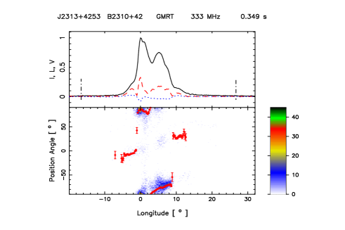
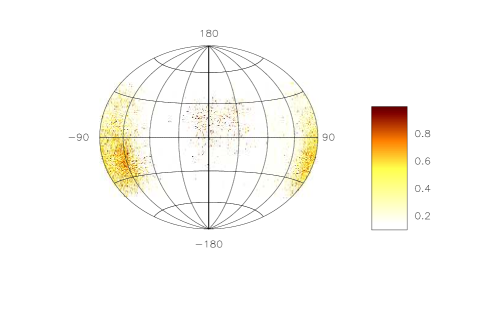
Figure 92: Top panel only at 333 MHz (upper window) shows the average profile with total intensity (Stokes I; solid black lines), total linear polarization (dashed red line) and circular polarization (Stokes V; dotted blue line). Top panel (lower window) also shows the single pulse PPA distribution (colour scale) along with the average PPA (red error bars). Bottom panel only at 333 MHz shows the Hammer-Aitoff projection of the polarized time samples with the colour scheme representing the fractional polarization level.

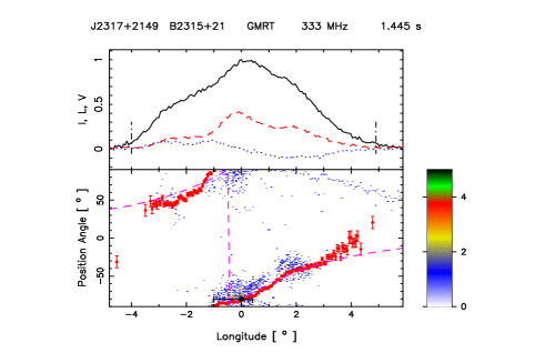
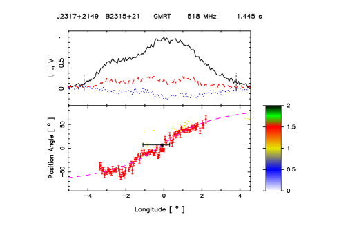
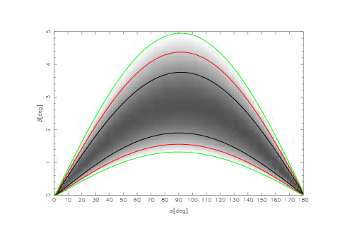
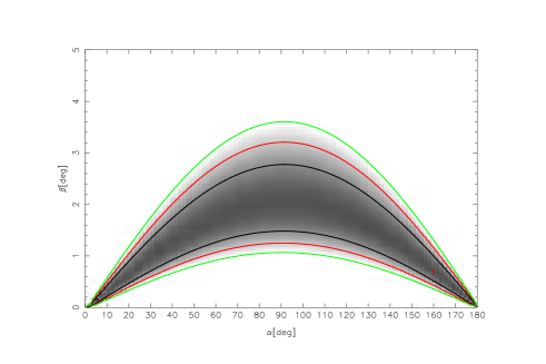
Figure 93: Top panel (upper window) shows the average profile with total intensity (Stokes I; solid black lines), total linear polarization (dashed red line) and circular polarization (Stokes V; dotted blue line). Top panel (lower window) also shows the single pulse PPA distribution (colour scale) along with the average PPA (red error bars). The RVM fits to the average PPA (dashed pink line) is also shown in this plot. Middle panel show the $\chi^{2}$ contours for the parameters $\alpha$ and $\beta$ obtained from RVM fits. Bottom panel shows the Hammer-Aitoff projection of the polarized time samples with the colour scheme representing the fractional polarization level.

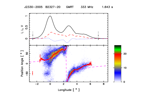
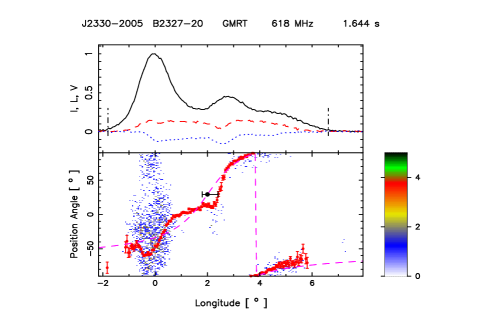
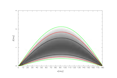
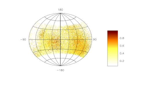
Figure 94: Top panel (upper window) shows the average profile with total intensity (Stokes I; solid black lines), total linear polarization (dashed red line) and circular polarization (Stokes V; dotted blue line). Top panel (lower window) also shows the single pulse PPA distribution (colour scale) along with the average PPA (red error bars). The RVM fits to the average PPA (dashed pink line) is also shown in this plot. Middle panel show the $\chi^{2}$ contours for the parameters $\alpha$ and $\beta$ obtained from RVM fits. Bottom panel shows the Hammer-Aitoff projection of the polarized time samples with the colour scheme representing the fractional polarization level.

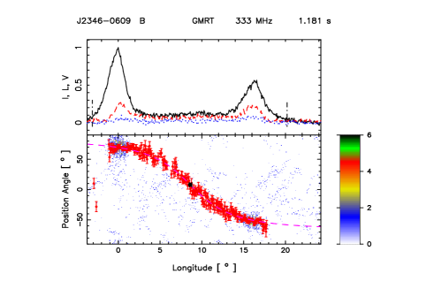
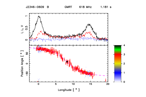
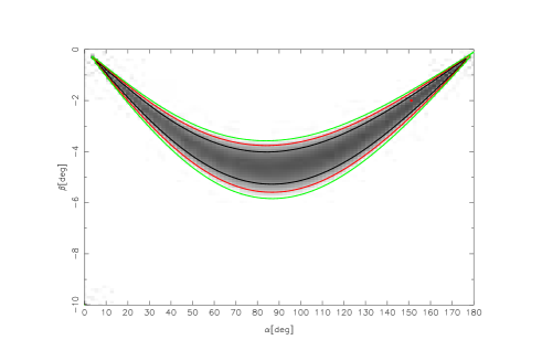
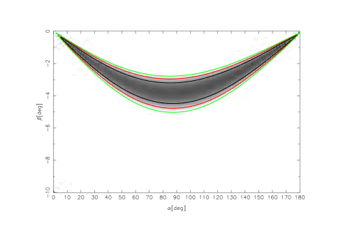
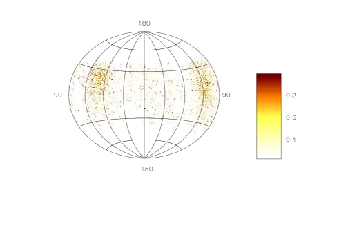
Figure 95: Top panel (upper window) shows the average profile with total intensity (Stokes I; solid black lines), total linear polarization (dashed red line) and circular polarization (Stokes V; dotted blue line). Top panel (lower window) also shows the single pulse PPA distribution (colour scale) along with the average PPA (red error bars). The RVM fits to the average PPA (dashed pink line) is also shown in this plot. Middle panel show the $\chi^{2}$ contours for the parameters $\alpha$ and $\beta$ obtained from RVM fits. Bottom panel shows the Hammer-Aitoff projection of the polarized time samples with the colour scheme representing the fractional polarization level.

References

• Allen & Melrose (1982) Allen, M. C., & Melrose, D. B. 1982, PASA, 4, 365, doi: 10.1017/S1323358000021147
• Arons & Barnard (1986) Arons, J., & Barnard, J. J. 1986, ApJ, 302, 120, doi: 10.1086/163978
• Asseo & Melikidze (1998) Asseo, E., & Melikidze, G. I. 1998, MNRAS, 301, 59, doi: 10.1046/j.1365-8711.1998.01990.x
• Basu et al. (2022a) Basu, R., Melikidze, G. I., & Mitra, D. 2022a, ApJ, 936, 35, doi: 10.3847/1538-4357/ac8479
• Basu et al. (2020a) Basu, R., Mitra, D., & Melikidze, G. I. 2020a, ApJ, 889, 133, doi: 10.3847/1538-4357/ab63c9
• Basu et al. (2020b) —. 2020b, MNRAS, 496, 465, doi: 10.1093/mnras/staa1574
• Basu et al. (2021) —. 2021, ApJ, 917, 48, doi: 10.3847/1538-4357/ac0828
• Basu et al. (2022b) —. 2022b, ApJ, 927, 208, doi: 10.3847/1538-4357/ac5039
• Basu et al. (2023) —. 2023, arXiv e-prints, arXiv:2303.12229, doi: 10.48550/arXiv.2303.12229
• Basu et al. (2016) Basu, R., Mitra, D., Melikidze, G. I., et al. 2016, ApJ, 833, 29, doi: 10.3847/1538-4357/833/1/29
• Basu et al. (2019) Basu, R., Mitra, D., Melikidze, G. I., & Skrzypczak, A. 2019, MNRAS, 482, 3757, doi: 10.1093/mnras/sty2846
• Blaskiewicz et al. (1991) Blaskiewicz, M., Cordes, J. M., & Wasserman, I. 1991, ApJ, 370, 643, doi: 10.1086/169850
• Cheng & Ruderman (1977) Cheng, A. F., & Ruderman, M. A. 1977, ApJ, 214, 598, doi: 10.1086/155285
• Cheng & Ruderman (1980) —. 1980, ApJ, 235, 576, doi: 10.1086/157661
• Everett & Weisberg (2001) Everett, J. E., & Weisberg, J. M. 2001, ApJ, 553, 341, doi: 10.1086/320652
• Gil et al. (2004) Gil, J., Lyubarsky, Y., & Melikidze, G. I. 2004, ApJ, 600, 872, doi: 10.1086/379972
• Gil et al. (2003) Gil, J., Melikidze, G. I., & Geppert, U. 2003, A&A, 407, 315, doi: 10.1051/0004-6361:20030854
• Gil & Rudnicki (1985) Gil, J., & Rudnicki, W. 1985, Ap&SS, 109, 381, doi: 10.1007/BF00651284
• Gil & Snakowski (1990) Gil, J. A., & Snakowski, J. K. 1990, A&A, 234, 269
• Ginzburg & Zhelezniakov (1975) Ginzburg, V. L., & Zhelezniakov, V. V. 1975, ARA&A, 13, 511, doi: 10.1146/annurev.aa.13.090175.002455
• Goldreich & Julian (1969) Goldreich, P., & Julian, W. H. 1969, ApJ, 157, 869, doi: 10.1086/150119
• Gould & Lyne (1998) Gould, D. M., & Lyne, A. G. 1998, MNRAS, 301, 235, doi: 10.1046/j.1365-8711.1998.02018.x
• Johnston & Kerr (2018) Johnston, S., & Kerr, M. 2018, MNRAS, 474, 4629, doi: 10.1093/mnras/stx3095
• Johnston et al. (2023) Johnston, S., Kramer, M., Karastergiou, A., et al. 2023, MNRAS, 520, 4801, doi: 10.1093/mnras/stac3636
• Karastergiou & Johnston (2007) Karastergiou, A., & Johnston, S. 2007, MNRAS, 380, 1678, doi: 10.1111/j.1365-2966.2007.12237.x
• Kazbegi et al. (1991) Kazbegi, A. Z., Machabeli, G. Z., & Melikidze, G. I. 1991, MNRAS, 253, 377, doi: 10.1093/mnras/253.3.377
• Kijak & Gil (1997) Kijak, J., & Gil, J. 1997, MNRAS, 288, 631, doi: 10.1093/mnras/288.3.631
• Lakoba et al. (2018) Lakoba, T., Mitra, D., & Melikidze, G. 2018, MNRAS, 480, 4526, doi: 10.1093/mnras/sty2152
• Lominadze et al. (1986) Lominadze, D. G., Machabeli, G. Z., Melikidze, G. I., & Pataraia, A. D. 1986, Fizika Plazmy, 12, 1233
• Manchester et al. (2005) Manchester, R. N., Hobbs, G. B., Teoh, A., & Hobbs, M. 2005, AJ, 129, 1993, doi: 10.1086/428488
• Manchester et al. (1975) Manchester, R. N., Taylor, J. H., & Huguenin, G. R. 1975, ApJ, 196, 83, doi: 10.1086/153395
• Manthei et al. (2021) Manthei, A. C., Benáček, J., Muñoz, P. A., & Büchner, J. 2021, A&A, 649, A145, doi: 10.1051/0004-6361/202039907
• Melikidze et al. (2000) Melikidze, G. I., Gil, J. A., & Pataraya, A. D. 2000, ApJ, 544, 1081, doi: 10.1086/317220
• Melikidze et al. (2014) Melikidze, G. I., Mitra, D., & Gil, J. 2014, ApJ, 794, 105, doi: 10.1088/0004-637X/794/2/105
• Melikidze & Pataraia (1980) Melikidze, G. I., & Pataraia, A. D. 1980, Astrofizika, 16, 161
• Melrose (1979) Melrose, D. B. 1979, Australian Journal of Physics, 32, 61, doi: 10.1071/PH790061
• Melrose (1995) —. 1995, Journal of Astrophysics and Astronomy, 16, 137, doi: 10.1007/BF02714830
• Mikhailovskii et al. (1982) Mikhailovskii, A. B., Onishchenko, O. G., Suramlishvili, G. I., & Sharapov, S. E. 1982, Soviet Astronomy Letters, 8, 369
• Mitra (2017) Mitra, D. 2017, Journal of Astrophysics and Astronomy, 38, 52, doi: 10.1007/s12036-017-9457-6
• Mitra et al. (2015) Mitra, D., Arjunwadkar, M., & Rankin, J. M. 2015, ApJ, 806, 236, doi: 10.1088/0004-637X/806/2/236
• Mitra et al. (2016) Mitra, D., Basu, R., Maciesiak, K., et al. 2016, ApJ, 833, 28, doi: 10.3847/1538-4357/833/1/28
• Mitra et al. (2020) Mitra, D., Basu, R., Melikidze, G. I., & Arjunwadkar, M. 2020, MNRAS, 492, 2468, doi: 10.1093/mnras/stz3620
• Mitra & Deshpande (1999) Mitra, D., & Deshpande, A. A. 1999, A&A, 346, 906. https://arxiv.org/abs/astro-ph/9904336
• Mitra et al. (2009) Mitra, D., Gil, J., & Melikidze, G. I. 2009, ApJ, 696, L141, doi: 10.1088/0004-637X/696/2/L141
• Mitra & Li (2004) Mitra, D., & Li, X. H. 2004, A&A, 421, 215, doi: 10.1051/0004-6361:20034094
• Mitra et al. (2023) Mitra, D., Melikidze, G. I., & Basu, R. 2023, MNRAS, doi: 10.1093/mnrasl/slad022
• Mitra & Rankin (2002) Mitra, D., & Rankin, J. M. 2002, ApJ, 577, 322, doi: 10.1086/342136
• Mitra & Rankin (2011) —. 2011, ApJ, 727, 92, doi: 10.1088/0004-637X/727/2/92
• Mitra & Seiradakis (2004) Mitra, D., & Seiradakis, J. H. 2004, in Hellenic Astronomical Society Sixth Astronomical Conference, ed. P. Laskarides, 205. https://arxiv.org/abs/astro-ph/0401335
• Morris et al. (1981) Morris, D., Graham, D. A., & Sieber, W. 1981, A&A, 100, 107
• Olszanski et al. (2019) Olszanski, T. E. E., Mitra, D., & Rankin, J. M. 2019, MNRAS, 489, 1543, doi: 10.1093/mnras/stz2172
• Pétri & Mitra (2020) Pétri, J., & Mitra, D. 2020, MNRAS, 491, 80, doi: 10.1093/mnras/stz2974
• Posselt et al. (2022) Posselt, B., Karastergiou, A., Johnston, S., et al. 2022, arXiv e-prints, arXiv:2211.11849, doi: 10.48550/arXiv.2211.11849
• Radhakrishnan & Cooke (1969) Radhakrishnan, V., & Cooke, D. J. 1969, Astrophys. Lett., 3, 225
• Rahaman et al. (2020) Rahaman, S. M., Mitra, D., & Melikidze, G. I. 2020, MNRAS, 497, 3953, doi: 10.1093/mnras/staa2280
• Rahaman et al. (2022a) —. 2022a, MNRAS, 512, 3589, doi: 10.1093/mnras/stac696
• Rahaman et al. (2022b) Rahaman, S. M., Mitra, D., Melikidze, G. I., & Lakoba, T. 2022b, MNRAS, 516, 3715, doi: 10.1093/mnras/stac2264
• Rankin (1983) Rankin, J. M. 1983, ApJ, 274, 333, doi: 10.1086/161450
• Rankin (1986) —. 1986, ApJ, 301, 901, doi: 10.1086/163955
• Rankin (1993) —. 1993, ApJ, 405, 285, doi: 10.1086/172361
• Ruderman & Sutherland (1975) Ruderman, M. A., & Sutherland, P. G. 1975, ApJ, 196, 51, doi: 10.1086/153393
• Shafranov (1967) Shafranov, V. D. 1967, Reviews of Plasma Physics, 3, 1
• Shapakidze et al. (2003) Shapakidze, D., Machabeli, G., Melikidze, G., & Khechinashvili, D. 2003, Phys. Rev. E, 67, 026407, doi: 10.1103/PhysRevE.67.026407
• Song et al. (2023) Song, X., Weltevrede, P., Szary, A., et al. 2023, arXiv e-prints, arXiv:2301.04067, doi: 10.48550/arXiv.2301.04067
• Sturrock (1971) Sturrock, P. A. 1971, ApJ, 164, 529, doi: 10.1086/150865
• Swarup et al. (1991) Swarup, G., Ananthakrishnan, S., Kapahi, V. K., et al. 1991, Current Science, 60, 95
• Volokitin et al. (1985) Volokitin, A. S., Krasnoselskikh, V. V., & Machabeli, G. Z. 1985, Fizika Plazmy, 11, 531
• von Hoensbroech & Xilouris (1997a) von Hoensbroech, A., & Xilouris, K. M. 1997a, A&A, 324, 981
• von Hoensbroech & Xilouris (1997b) —. 1997b, A&AS, 126, 121
• Wang et al. (2010) Wang, C., Lai, D., & Han, J. 2010, MNRAS, 403, 569, doi: 10.1111/j.1365-2966.2009.16074.x
• Weltevrede et al. (2006) Weltevrede, P., Edwards, R. T., & Stappers, B. W. 2006, A&A, 445, 243, doi: 10.1051/0004-6361:20053088
• Weltevrede & Johnston (2008) Weltevrede, P., & Johnston, S. 2008, MNRAS, 391, 1210, doi: 10.1111/j.1365-2966.2008.13950.x