Contagion Effect Estimation Using Proximal Embeddings

Abstract.

Contagion effect refers to the causal effect of peers’ behavior on the outcome of an individual in social networks. Contagion can be confounded due to latent homophily which makes contagion effect estimation very hard: nodes in a homophilic network tend to have ties to peers with similar attributes and can behave similarly without influencing one another. One way to account for latent homophily is by considering proxies for the unobserved confounders. However, as we demonstrate in this paper, existing proxy-based methods for contagion effect estimation have a very high variance when the proxies are high-dimensional. To address this issue, we introduce a novel framework, Proximal Embeddings (ProEmb), that integrates variational autoencoders with adversarial networks to create low-dimensional representations of high-dimensional proxies and help with identifying contagion effects. While VAEs have been used previously for representation learning in causal inference, a novel aspect of our approach is the additional component of adversarial networks to balance the representations of different treatment groups, which is essential in causal inference from observational data where these groups typically come from different distributions. We empirically show that our method significantly increases the accuracy and reduces the variance of contagion effect estimation in observational network data compared to state-of-the-art methods.

Introduction

The goal of causal inference is to estimate the effect of an intervention on individuals’ outcomes. Traditionally, causal inference has relied on the assumption of no interference, which states that any individual’s response to treatment depends only on their own treatment and not on the treatment of others. However, individuals can impact each other through their interactions. Contagion is a type of interference that is defined as the influence of neighbors’ actions on the actions of an individual. Contagion effect estimation plays a central role in understanding how social environments shape personal actions, behavior, and attitudes (Fowler and Christakis, 2008; Bramoullé et al., 2009; Eckles et al., 2016). Some real-world applications of contagion effect estimation include studying the spread of obesity from one person to another (Christakis and Fowler, 2007; Krauth, 2005), analyzing the spread of smoking behavior among peers (Christakis and Fowler, 2008), and understanding the role of one’s social environment in trusting fake news on online social media platforms (Torres et al., 2018).

Despite their importance, identification (i.e. determining causal estimands based on observational data distribution (Pearl, 2009)) and estimation of contagion effects are challenging due to the presence of unmeasured confounders, variables that affect both the treatment and the outcome of interest. A common source of confounding in networks is latent homophily (Shalizi and Thomas, 2011; Manski, 1993; VanderWeele and An, 2013; Ogburn et al., 2017), the tendency of ties to form between individuals with similar unobserved attributes. When contagion effects are confounded with latent homophily, it is hard to tell if any changes in the individual’s outcome are the result of neighbors’ influence or the similarity between the individual and neighbors characteristics. For example, people with similar political affiliations would be more likely to interact on social media (e.g., Twitter) and they may express similar opinions (e.g., agree or disagree with social distancing policies during a pandemic), not because one influences the other but because they share similar political views in the first place.

To identify and estimate contagion effects in the presence of unobserved confounders, existing approaches look for observed variables that can be considered as valid proxies of the unobserved confounders (Miao et al., 2018; Tchetgen et al., 2020; Egami and Tchetgen, 2021). However, such approaches can perform poorly on real-world observational data, such as web and social media, in which a high-dimensional covariate space is the norm. High-dimensional control proxies (e.g., tweet words of a user) lead to a sparse vector of model parameters and higher asymptotic bias and variance of the estimation (De Luna et al., 2011). Another source of variance is selection bias (Guo et al., 2020; Shalit et al., 2017; Assaad et al., 2021; Johansson et al., 2016). Selection bias occurs when there is a mismatch in attribute distribution between the treatment and control groups. For instance, a treatment group can comprise mostly individuals who prioritize their health and have friends who follow social distancing guidelines, while the control group comprises of individuals who do not prioritize their health and have friends who largely disregard social distancing measures. A common method for dealing with selection bias in observational studies is matching, where a balanced sample is created by identifying similar units from the opposite treatment group. However, matching tends to encounter scalability issues when applied to high-dimensional data (Abadie and Imbens, 2006; Assaad et al., 2021).

To address high-dimensionality and selection bias in real-world contagion estimation settings, we introduce Proximal Embeddings (ProEmb), a framework for inferring contagion effects in homophilic networks. ProEmb learns embeddings of high-dimensional proxies for unobserved confounders. It combines variational autoencoders (VAEs) and adversarial networks (Goodfellow et al., 2014; Mescheder et al., 2017) to map high-dimensional proxies to a probability distribution over the latent space with the goal of obtaining a balanced low-dimensional proxy representation. While the use of VAEs for causal effect estimation is not new  (Louizos et al., 2017; Grari et al., 2022; Kim et al., 2021; Im et al., 2021), our framework has two novel components. The first one is in defining and developing the first solution to the problem of contagion estimation with high-dimensional proxies, an important problem in real-world contagion estimation scenarios. The second one is the novel enhancement of VAEs with adversarial networks, similar to matching  (Stuart, 2010), which play the important role of addressing the selection bias in treatment groups and is of independent interest for causal effect estimation beyond contagion. In addition to being meaningful for causal inference, this enhancement is crucial for the empirical performance of the estimator.

Our framework consists of three main components: 1) an embedding learning component that maps high-dimensional proxies to low-dimensional latent representations, 2) a representation balancing component that addresses the representation mismatch between treatment and control groups in the learned latent space, and 3) a counterfactual learning component, where an outcome model is trained to infer the potential outcomes of nodes based on the treatment and the low-dimensional representation of proxies. The primary goal of dimensionality reduction is to reduce bias and variance in the estimation by decreasing sparsity and the number of model parameters that need to be estimated.

Key idea and highlights. To summarize, this paper makes the following main contributions:

• We formulate the problem of contagion effect estimation in networks when latent homophily and high-dimensional proxies of latent confounders are present.

• We propose a novel framework for contagion effect estimation, ProEmb, that integrates VAEs, adversarial networks, and meta-learners for balanced representation learning and contagion effect estimation.

• Through empirical analysis, we demonstrate that existing methods for inferring contagion effects using high-dimensional proxies are prone to high bias and variance, while our proposed approach exhibits remarkable performance improvements over state-of-the-art techniques.

Related Work

Here, we review prior studies that focus on causal inference in observational network data. Ogburn and VanderWeele (2014) study the role of structural causal models in causal effect estimation in the presence of different types of interference. Shalizi and Thomas (2011) show that in networks formed by latent homophily, contagion, and homophily can be confounded and the causal effect is not always identifiable. Another study shows that controlling for the cluster assignment of nodes can help (Shalizi and McFowland III, 2016). A recent study deploys negative control outcome and exposure variables to estimate contagion effects in low-dimensional settings (Egami and Tchetgen, 2021). Our work builds upon this work and focuses on estimating contagion effects in datasets with high-dimensional proxies.

Recently, a series of methods have been proposed to leverage representation learning to relax the strong ignorability assumption in networked data. Guo et al. (2020) propose the Network Deconfounder framework where network structure and the observed features of nodes are mapped to a latent representation space to capture the influence of hidden confounders. Veitch et al. (2019) propose a procedure for estimating treatment effects using network embeddings by reducing the causal estimation problem to a semi-supervised prediction of the treatments and outcomes and using embedding models for the semi-supervised prediction. Cristali and Veitch (2021) use node embeddings learned from the network structure for estimating contagion effects in a different setting where covariates and the network structure are unobserved. However, these works either do not consider interference (Guo et al., 2020; Veitch et al., 2019), or selection bias (Cristali and Veitch, 2021).

Methods to improve the distribution mismatch between treatment groups include combining weighting with representation learning (Hassanpour and Greiner, 2019; Li and Fu, 2017; Guo et al., 2020), linear ridge regression with representation learning (Jiang and Sun, 2022a), and a discriminator component that balances the representation of the observed confounders (Jiang and Sun, 2022a). Our approach is distinct in that it balances the proxy representations generated by VAEs with adversarial networks.

Several studies have utilized VAEs to estimate proxies for confounding variables in non-network data. Louizos et al. (Louizos et al., 2017) leverage VAEs for the purpose of inferring latent variables proxies that help with estimating individual treatment effects. Grari et al. (Grari et al., 2022) integrate VAEs with an adversarial training component aimed at acquiring a proxy for latent sensitive information, such as gender. Their approach differs from our framework in the sense that adversarial training focuses on guaranteeing the independence of the generated latent space from the unobserved sensitive variable. In contrast, our approach utilizes the discriminator component of an adversarial network to achieve a balance in the representation of treatment and control groups.

Problem Description

In this section, we present our data and causal model, the causal estimand, different types of proxy variables, and issues with contagion effect estimation in high-dimensional settings.

Data model

We assume a graph $G=(\mathbf{V},\mathbf{E})$ that consists of a set of $|\mathbf{V}|$ nodes and a set of edges $\mathbf{E}=\{e_{ij}\}$, where $e_{ij}$ denotes that there is an edge between node $v_{i}\in\mathbf{V}$ and node $v_{j}\in\mathbf{V}$. Each node has an observed $n$-dimensional vector of attributes, $\mathbf{Z}_{i}$, unobserved characteristics, $\mathbf{U}_{i}$, and outcomes in two consecutive time steps, $Y_{i,t-1}\in\{0,1\}$, and $Y_{i,t}\in\mathbb{R}$. If node $v_{i}$ is activated at time $t-1$ (e.g., obeyed social distancing policies), then $Y_{i,t-1}=1$. Let $\mathbf{N}_{i}=\{v_{j}|v_{j}\in\mathbf{V}\ \ \&\ \ \exists\ \ e_{ij}\in\mathbf{E}\}$ denote the set of neighbors of node $v_{i}$ and $\mathbf{A}_{i}$ be the adjacency vector for node $v_{i}$ where $A_{ij}=1$ if $\exists e_{ij}$. For each node, there exists a set of neighbors’ hidden characteristics $\mathbf{U}_{ngb}$, a set of neighbors’ observed attributes $\mathbf{Z}_{ngb}$, and two sets of neighbors’ outcomes $\mathbf{Y}_{ngb,t-1}$ and $\mathbf{Y}_{ngb,t}$. We further assume that edges form by latent homophily on $\mathbf{U}$ which means that nodes with more similar unobserved characteristics are more likely to connect  (Shalizi and McFowland III, 2016).

Causal Model

Following Egami and Tchetgen (2021), we assume the causal graph depicted in Fig. 1, where the connections are formed based on the similarity of the unobserved homophilic attributes. However, Egami and Tchetgen consider a chain graph (Lauritzen and Richardson, 2002) to represent network dependence of unobserved confounders across units. Hidden variables are represented by dashed circles.

In each connection, ”ego” refers to a node whose contagion effects we estimate, and ”peer” refers to a node that influences the ego’s outcome. In this paper, treatment is the set of peer outcomes $\mathbf{Y}_{ngb,t-1}$ and the outcome is the ego’s outcome $Y_{i,t}$. The potential outcome of node $v_{i}$ under contagion effects is defined as the value that $Y_{i,t}$ would take if peer’s outcome $\mathbf{Y}_{ngb,t-1}$ had been set to $y$. The factual outcome $Y_{i,t}^{F}$ refers to the observed outcome of an individual when $\mathbf{Y}_{ngb,t-1}=y$ and the counterfactual outcome $Y_{i,t}^{CF}$ shows the unobserved response of an individual when $\mathbf{Y}_{ngb,t-1}=1-y$.

Given a set of activated neighbors $\hat{\mathbf{N}}_{i}\subseteq\mathbf{N}_{i}$, we define $h:\{0,1\}^{|\mathbf{N}_{i}|}\rightarrow\{0,1\}$ as a function over the neighbors’ activations which maps the neighbors’ activations to a binary value. In this paper, we consider the ego-networks connection model where multiple activated peers may exist ($|\mathbf{N}_{i}|\geq 1$). Dyads, i.e., pairs of two individuals, are a special case of the ego-networks model where for every node $v_{i}$, $|\mathbf{N}_{i}|=1$ and an activated peer can activate an ego.

Contagion Effect Estimation

We define Individual Contagion Effects (ICE) as the difference between the outcome of node $v_{i}$ under two different values for the neighbors’ activation $h(\mathbf{Y}_{ngb,t-1})$:

(1) $$\tau_{i}=Y_{i,t}(h(\mathbf{Y}_{ngb,t-1})=1)-Y_{i,t}(h(\mathbf{Y}_{ngb,t-1})=0)$$

Our objective is to estimate ACE, which represents the average of ICE over all nodes. In observational data, estimating ICE is challenging because we can never simultaneously observe the factual and counterfactual outcomes of a unit.

One of the main assumptions in inferring causal effects from observational data is strong ignorability or no unmeasured confounding. According to this condition, the potential outcomes of a node are independent of its treatment assignment given its observed attributes (Rosenbaum and Rubin, 1983). Under the strong ignorability assumption, adjusting for variables that block the back-door path allows for the identification of the causal effect (Pearl, 2009). A back-door path refers to a path from treatment to outcome in the structural causal model that has an arrow into the treatment variable. When unblocked back-door paths exist, there are two sources of association between treatment and outcome: one is causal (the causal effect of treatment on the outcome), and the other is non-causal (through the back-door path). In the presence of unblocked back-door paths, it becomes challenging to decide whether the observed association is a result of the causal effect or the spurious association enabled by the back-door path. In the causal model represented in Fig. 1, strong ignorability holds if:

(2) $$Y_{i,t}(1),Y_{i,t}(0)\perp\!\!\!\perp\mathbf{Y}_{ngb,t-1}\mid\mathbf{Z}_{i},\mathbf{A}_{i}.$$

Figure 1. The causal model for the ego-network of ego $v_{i}$: $\mathbf{Z}_{i}$ and $\mathbf{Z}_{ngb}$ are proxies of the hidden confounders. $\mathbf{U}_{i}$ and $\mathbf{U}_{ngb}$ are unobserved homophilic attributes. Dashed circles show unobserved variables.

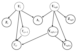
However, conditioning on $\mathbf{A}_{i}$ introduces a dependence association between unobserved variables $\mathbf{U}_{i}$ and $\mathbf{U}_{ngb}$ where the unblocked backdoor path $Y_{i,t}\leftarrow\mathbf{U}_{i}\rightarrow\mathbf{A}_{i}\leftarrow\mathbf{U}_{ngb}\rightarrow\mathbf{Y}_{ngb,t-1}$ violates the ignorability assumption ($Y_{i,t}\not\!\perp\!\!\!\perp\mathbf{Y}_{ngb,t-1}|\mathbf{A}_{i},\mathbf{Z}_{i}$) and makes the contagion effects unidentifiable. We are interested in measuring ACE in the presence of an unobserved confounder, i.e., where the unobserved network confounder is the direct cause of the outcome of an ego and its peers.

Double Negative Control Proxies

One way to account for latent homophily is by considering proxies for unobserved confounders. Proxies are measurable variables that are correlated with the unobserved variable, and conditioning on them enables the identification of the causal effect (Miao et al., 2018). Negative controls are two groups of common proxies that make the causal effect identifiable in settings with unobserved confounders: 1) Negative Control Exposure (NCE) is a treatment variable that does not causally affect the outcome of interest, and 2) Negative Control Outcome (NCO) is a variable that is not causally affected by the treatment of interest. NCE and NCO correspond to proxy types b and c, respectively. (Egami and Tchetgen, 2021) demonstrate that leveraging these two types of negative control proxies can enable the identification of contagion effects in networked data with unobserved confounders. In the causal model presented in Fig. 1, a variable $\mathbf{Z}_{i}$ is considered as an NCO if:

(3) $$\mathbf{Z}_{i}\perp\!\!\!\perp\mathbf{Y}_{ngb,t-1}|\mathbf{U}_{i},\mathbf{U}_{ngb},\mathbf{A}_{i}$$

and variable $\mathbf{Z}_{ngb}$ is considered as an NCE if:

(4) $$\mathbf{Z}_{ngb}\perp\!\!\!\perp Y_{i,t}|\mathbf{Y}_{ngb,t-1},\mathbf{U}_{i},\mathbf{U}_{ngb},\mathbf{A}_{i},$$

(5) $$\mathbf{Z}_{ngb}\perp\!\!\!\perp\mathbf{Z}_{i}|\mathbf{Y}_{ngb,t-1},\mathbf{U}_{i},\mathbf{U}_{ngb},\mathbf{A}_{i}.$$

Assumption 3 implies that the variable $\mathbf{Z}_{i}$ serves as an auxiliary variable which is independent of the treatment, given the unobserved confounders and the adjacency vector of the node. Assumptions 4 and 5 consider $\mathbf{Z}_{ngb}$ as an auxiliary variable, independent of the outcome and NCO, given treatment, unobserved confounders, and the adjacency vector.

Various estimators can be employed to infer the causal effect of interest using proxies. One commonly used approach is the Two-stage Least Squares estimator (TSLS). TSLS consists of two stages (Angrist and Imbens, 1995). First, a new variable is constructed using the instrumental variables. This variable serves as a proxy for the unobserved confounders. Then, the estimated values obtained from the first stage are utilized in place of the unobserved confounders, and an Ordinary Least Squares regression (OLS) is performed to estimate the causal effect.  (Egami and Tchetgen, 2021) employ the TSLS estimator to quantify contagion effects by leveraging the NCE and NCO proxies as:

(6) $$Y_{i,t}\sim\mathbf{Y}_{ngb,t-1}+\mathbf{Z}_{i}|\mathbf{Z}_{ngb}+\mathbf{Y}_{ngb,t-1}$$

where the coefficient of $\mathbf{Y}_{ngb,t-1}$ shows the estimated ACE.

Issues with high-dimensional proxies

High-dimensional datasets are characterized by a large number of attributes, such as customers’ extensive purchase history in recommender systems. In the presence of high-dimensional data, the number of model parameters $p$ exceeds the number of data samples $n$, a problem known as the “Large $p$ Small $n$” issue in causal effect estimation using regression models (Bernardo et al., 2003). Estimating contagion effects using control proxies can be problematic when the NCO and NCE proxies are high-dimensional because the matrix of model parameters becomes sparse and exhibits a low-rank structure (Deaner, 2021). A matrix is considered low-rank if the number of linearly independent variables is significantly smaller than the total number of variables. Including correlated variables in the estimation process increases the variance of the causal estimand (Abadie and Imbens, 2006; De Luna et al., 2011), which adversely affects the performance of the estimator (Chao and Swanson, 2005; Hansen et al., 2008). This issue becomes even more prominent in TSLS estimation, where the computational burden increases with the number of instruments or predictors.

Besides high dimensionality, selection bias can be another source of high variance for the causal effect estimate. This bias arises due to a mismatch in the distribution of attributes between the treatment and control groups. In the presence of selection bias, the observed differences between the outcome of treatment and control nodes may be due to the difference between their attributes rather than the true treatment effect.

The goal of this paper is to solve the following problem:

Problem 1 (Contagion Effect Estimation with High-dimensional Proxies).

Let $G=(\bm{V},\bm{E})$ be a graph evolved by latent homophily with high-dimensional double negative control proxies, associated with nodes. Our goal is to find an estimate of the average contagion effect (ACE) $\hat{\theta}$ that minimizes the expected error between $\hat{\theta}$ and the true value of ACE $\theta$.

Proximal Embedding Framework for Contagion Effect Estimation

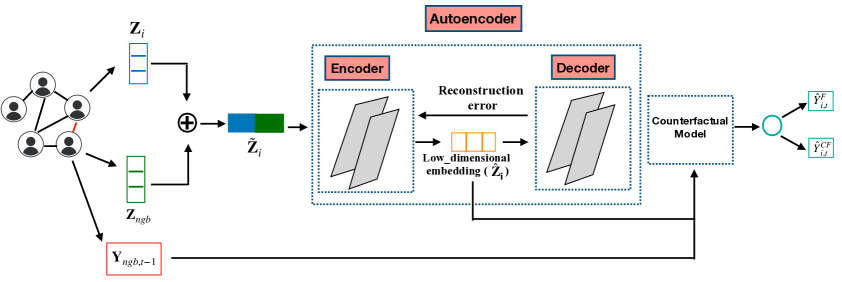
To address high dimensionality and selection bias in contagion effect estimation, we introduce the Proximal Embeddings (ProEmb) framework. ProEmb has three main components, shown in Fig. 2. The first component tackles issues of sparsity and high dimensionality by reducing dependent variables to uncorrelated ones, thereby improving estimator optimality (Wang et al., 2014; De Luna et al., 2011). A key technique for this is variational autoencoders (VAEs) (Kingma and Welling, 2014; Rezende et al., 2014), which represent inputs as distributions in a latent space and enforce regularization by ensuring encoder-generated distributions closely resemble a Gaussian distribution.

However, simply applying VAEs to causal inference is not sufficient because embeddings generated by VAEs can vary across different treatment groups and it can lead to confounding biases in estimating causal effects. To address this problem, the second component of ProEmb integrates adversarial networks to update the generated representation by VAEs and improve the distribution shift between the representation of treatment and control node proxies. This updated representation is then passed on to the third component which consists of a counterfactual learning module that measures counterfactual outcomes using meta-learners (Künzel et al., 2019). To the best of our knowledge, ProEmb is the first method that integrates VAEs, adversarial networks, and meta-learners to improve causal effect estimation more generally, and more specifically contagion effect estimation in networks with unobserved confounders. Next, we describe each component in more detail.

Figure 2. Illustration of the ProEmb framework with three components: 1) embedding learning where VAEs are used to generate low-dimensional embeddings of the proxies, 2) representation balancing where adversarial networks are used to improve the proxy representation mismatch between treatment groups, and 3) counterfactual model where an estimator is trained to predict the counterfactual outcomes.

Embedding learning

The goal of this component is learning a low-dimensional representation of high-dimensional and sparse proxies while preserving the parts of proxies that are predictive of the outcomes. We assume that the experimenter has classified observed variables into NCO and NCE proxies based on assumptions 3-5. We use VAEs to learn low-dimensional representations for each node’s proxies. VAEs have demonstrated remarkable success in dimensionality reduction due to their ability to both capture the underlying structure of high-dimensional data and regularize the latent space, which helps to prevent overfitting and improve generalization performance  (Gregor et al., 2015; Jimenez Rezende et al., 2016; Pu et al., 2016; Portillo et al., 2020).

In order to adapt VAEs to the problem of contagion estimation with high-dimensional proxies, one has to be careful to consider 1) how to capture latent homophily, 2) how to sample diverse low-dimensional representations from the representation space during training and inference, and 3) how to reconstruct the original high-dimensional proxy vectors, in order to evaluate and improve the performance of the model. ProEmb’s variational autoencoder addresses these considerations through each of its three parts:

1. Probabilistic Encoder. This component transforms high-dimensional proxies into a distribution in the latent space to infer the unobserved confounders. Since $\mathbf{Z}_{i}$ as an NCO and $\mathbf{Z}_{ngb}$ as an NCE variable are proxies of the unobserved homophilic attributes, we expect to recover latent features by applying a well-trained encoder model to the concatenation of these proxies. Let $\mathbf{\tilde{Z}}_{i}=\{z_{i,1},...,z_{i,n},z_{ngb,1},\allowbreak...,z_{ngb,n}\}$ denote the concatenated vector of proxies $\mathbf{Z}_{i}=\{z_{i,1},...,z_{i,n}\}$ and $\mathbf{Z}_{ngb}=\{z_{ngb,1},...,z_{ngb,n}\}$ with dimension $n$. We use the encoder layer with $L$ fully-connected layers to map proxies $\mathbf{\tilde{Z}}_{i}$ to low-dimensional latent vector $\mathbf{Z^{\prime}}_{i}$ as:

   (7) $$\mathbf{Z^{\prime}}_{i}=g(\mathbf{W}_{l}...g(\mathbf{W}_{1}\mathbf{\tilde{Z}}_{i})),$$

   where $g$ indicates the activation function (e.g., Relu) and $\{\mathbf{W}_{l}\},l\in\{1,...,L\}$ represents the weight matrices of the fully connected layers of the encoder.

2. Sampler. The sampler plays a crucial role in generating latent vectors from the learned distribution in the latent space. These vectors are randomly sampled from the distribution $p(\mathbf{\hat{Z}}_{i}|\mathbf{\tilde{Z}}_{i})$, utilizing the mean and log-variance values obtained from the encoder’s output. The latent layer is represented by two sets of neurons: one set representing the means of the latent space, and the other set representing the log-variances, measured as:

   (8) $$\mu =\mathbf{W_{\mu}\mathbf{Z^{\prime}}_{i}}+\mathbf{b^{\mu}},$$

   (9) $$ln\,\delta^{2} =\mathbf{W_{\delta}\mathbf{Z^{\prime}}_{i}}+\mathbf{b^{\delta}},$$

   where $\mathbf{b^{\mu}}$ and $\mathbf{b^{\delta}}$ are vectors of biases. A proxy representation is sampled from the latent space as:

   (10) $$\mathbf{\hat{Z}}_{i}\sim p(\mathbf{\hat{Z}}_{i}|\mathbf{\tilde{Z}}_{i})=\mathcal{N}(\mu,exp(ln\ \ \delta^{2})).$$

   $\mathbf{\hat{Z}}_{i}$ contains the low-dimensional representation of the proxies which is later used by the counterfactual learning component for contagion effect estimation.

3. Probabilistic Decoder. The decoder attempts to reconstruct the original proxy vector $\mathbf{\tilde{Z}}_{i}$ from the proxy representation $\mathbf{\hat{Z}_{i}}$. The decoder uses $\hat{L}$ fully-connected layers to map $\mathbf{\hat{Z}_{i}}$ to $\mathbf{\tilde{Z}_{i}}$, i.e.,

   (11) $$\mathbf{Z}_{i}^{\prime\prime}=f(\mathbf{\hat{W}}_{l}...f(\mathbf{\hat{W}}_{1}\mathbf{\hat{Z}}_{i})),$$

   where $\mathbf{Z}_{i}^{\prime\prime}$ shows the reconstructed representation, $f$ indicates the activation function, and $\{\mathbf{\hat{W}}_{l}\},l\in{1,...,\hat{L}}$ denotes the weight matrix of the fully connected layers.

The loss function of VAEs consists of two main parts: 1) the reconstruction loss which measures the dissimilarity between the original data and the data reconstructed by the VAEs, and 2) the Kullback–Leibler (KL) divergence (Kullback and Leibler, 1951) which is a regularizer and quantifies the discrepancy between the inferred distribution $p(\mathbf{\hat{Z}}|\mathbf{\tilde{Z}})$ and the known distribution $p(\mathbf{\tilde{Z}})$. The loss function of VAEs is defined as:

(12) $$\mathcal{L}_{vae}=\frac{1}{|\mathbf{V}|}\sum_{i=1}^{|\mathbf{V}|}{|{z^{\prime}_{i}}-z_{i}|^{2}}+KL(p(\mathbf{\hat{Z}}_{i}|\mathbf{\tilde{Z}}_{i})|p(\mathbf{\tilde{Z}}_{i}))_{i=1}^{|\mathbf{V}|}.$$

Representation balancing

Since the embedding learning models are trained on the factual outcomes and used to predict the counterfactual outcomes, minimizing the error in factual outcomes $Y^{F}_{i,t}$ does not guarantee the simultaneous error reduction in counterfactual outcomes $Y^{CF}_{i,t}$. Therefore, it is crucial to develop a model that tackles the distribution mismatch between treatment and control nodes in terms of their proxy representations. In this particular component, our focus is on enhancing proxy representation to achieve similarity between the induced distributions for treated and control nodes. Inspired by (Jiang and Sun, 2022b), we employ the discriminator component of Generative Adversarial Networks (Goodfellow et al., 2014) to address the imbalance proxy representations generated by VAEs.

Let $\mathcal{D}:\mathbf{\hat{Z}}_{i}\rightarrow\{0,1\}$ denote the discriminator function, mapping the latent representation $\mathbf{\hat{Z}}_{i}$ to $Y_{i,t-1}$. Initially, we train the discriminator to maximize the probability of accurately predicting $Y_{i,t-1}$ from the latent representation. This is achieved by optimizing the discriminator loss function:

(13) $$\mathcal{L}_{\mathcal{D}} =\frac{1}{|\mathbf{V}|}\sum_{i=1}^{|\mathbf{V}|}(Y_{i,t-1}\ log\ \mathcal{D}(\hat{\mathbf{Z}}_{i})$$

$$+(1-Y_{i,t-1})\ log(1-\mathcal{D}(\hat{\mathbf{Z}}_{i})).$$

We update the latent representation $\mathbf{\hat{Z}}_{i}$ such that the distribution $p(Y_{i,t-1}|\mathbf{\hat{Z}}_{i})$ becomes uniform. Considering that $Y_{ngb,t-1}$ is binary, a uniform distribution implies that $p(Y_{ngb,t-1}=1|\mathbf{\hat{Z}}_{i})=p(Y_{ngb,t-1}=0|\mathbf{\hat{Z}}_{i})=0.5$. The $p(Y_{ngb,t-1}|\mathbf{\hat{Z}}_{i})$ regularization loss is defined as:

(14) $$\mathcal{L}_{rb}=\frac{1}{|V|}\sum_{i=1}^{|V|}{(\mathcal{D}(\mathbf{\hat{Z}}_{i})-0.5)^{2}}.$$

The regularization loss $\mathcal{L}_{rb}$ is then backpropagated to the encoding part of the VAEs, enabling the update of the latent representation $\mathbf{\hat{Z}}_{i}$ such that the discriminator $\mathcal{D}$ cannot accurately predict $Y_{ngb,t-1}$. This leads to a more balanced and unbiased latent representation for proxies.

Counterfactual learning

This component focuses on training a model to infer the counterfactual outcomes from low-dimensional embeddings of proxies $\mathbf{\hat{Z}_{i}}\in R^{m}$ as well as the peers’ outcome $\mathbf{Y}_{ngb,t-1}$. The factual outcomes are used to train the model. The objective function of this component during training is to minimize the error of the inferred factual outcomes defined as $\frac{1}{n}\sum_{i=1}^{n}{(\hat{Y}_{i,t}-Y_{i,t})}^{2}$ where $\hat{Y}_{i,t}$ indicates the predicted factual outcome by ProEmb.

We assume that the proxy representation is sufficiently informative to satisfy the strong ignorability assumption ($Y_{i,t}\!\perp\!\!\!\perp\mathbf{Y}_{ngb,t-1}|\mathbf{\hat{Z}_{i}}$), which allows us to make counterfactual predictions. To make this process more concrete, we demonstrate how our framework would use a common Heterogeneous Treatment Effect (HTE) estimation algorithm, the T-learner. However, our framework could leverage other HTE estimation algorithms as well. T-learner meta-learning algorithm is an example of such estimators and is used to measure Conditional Average Treatment Effect (CATE). A meta-learner is a framework to estimate the Individual Treatment Effects (ITE) using any supervised machine learning estimators known as base-learners  (Künzel et al., 2019). In T-learner, two base-learners are trained with treatment ($\mu_{t}$) and control nodes ($\mu_{c}$) to estimate the conditional expectations of the outcomes given observed attributes. $\mu_{t}$ is employed to predict the counterfactual outcomes of control nodes, and $\mu_{c}$ is used to predict the counterfactual outcomes of treatment nodes. The difference between the predicted outcomes by treatment and control models show ITE. A T-learner has the advantage of simplicity and adaptability, as it utilizes any machine learning model as a base-learner.

Experiments

In this section, we evaluate the performance of different methods for contagion effect estimation on semi-synthetic datasets. We also demonstrate the applicability of our approach for detecting contagion effects in a Twitter dataset about the 2017 French presidential election (Burghardt et al., 2023) and a Peer Smoking dataset (Mermelstein et al., 2009).

Semi-synthetic data generation

As ground truth for causal effects is unavailable in real-world datasets, researchers commonly rely on synthetic and semi-synthetic datasets to evaluate causal inference methods. In this section, we describe the semi-synthetic datasets we generated for our experiments. It is important to note that the generation doesn’t consider embeddings and is therefore not biased towards an embedding-based solution. We utilize four real-world datasets: 1) Hateful Users, which is a sample of 5,000 hateful and normal tweets (Ribeiro et al., 2018), 2) Stay-at-Home (SAH), which is a sample of 30,000 tweets reflecting users’ attitudes toward stay-at-home orders during the COVID-19 pandemic (Fatemi et al., 2022), 3) BlogCatalog, which is a sample of 5,196 bloggers from an online community where users post blogs (Guo et al., 2020), and 4) Flickr which is a sample of 7,575 users who share photos on Flickr online social media platform (Guo et al., 2020). In the first two datasets, each tweet exhibits a unique distribution over several topics, reflecting the hidden semantic structure of the tweet. We consider the topic distribution of each tweet as the unobserved confounder $\mathbf{U}_{i}$. To extract the topic distribution of each tweet, we employ Latent Dirichlet Allocation (LDA) (Blei et al., 2003) and measure the coherence score to determine the optimal number of topics. We obtain 20 topics for SAH and 50 topics for the Hateful Users dataset. For the BlogCatalog and Flickr datasets, we follow (Guo et al., 2020) and learn 50 topics. More dataset details are in the Appendix.

Ego-networks model. Since our causal model relies on the assumption that ties form between nodes by latent homophily, we generate the networks synthetically. We consider data on both networks and dyads and generate ties between nodes based on latent homophily. The advantage of considering both dyadic and network data is that it allows us to examine scenarios where a node is influenced by either a single activated neighbor or multiple activated neighbors. By considering dyadic data, we can focus on the interactions between pairs of nodes and gain insights into how one node’s activation affects its immediate neighbor. This analysis provides valuable information about the dynamics at the micro-level. On the other hand, analyzing network data allows us to capture the broader influence of multiple activated neighbors on a node.

In the dyadic model, each node in the graph is connected to only one other node. The probability of an edge forming between node $v_{i}$ and $v_{j}$ is determined by the cosine similarity of their latent attribute vectors $\mathbf{U}_{i}$ and $\mathbf{U}_{j}$. This means that individuals with similar latent attributes are more likely to be connected.

In the network model, we aim to generate networks growing based on latent homophily and preferential attachment. We start with $m_{0}=3$ fully connected seed nodes. At each time step, a new node $v_{j}$ connects to $m=3$ existing nodes, selected randomly with a probability proportional to the node’s degree ( (Piva et al., 2021)):

(15) $$\pi(k_{i}|j)=\frac{\cos(\mathbf{U}_{i},\mathbf{U}_{j})k_{i}}{\sum_{n}\cos(\mathbf{U}_{i},\mathbf{U}_{n})k_{n}}.$$

In our network model, we assume that activated neighbors may activate an inactivated ego with the probability of $0.3$. In the Supplement, we also show results for a different model that focuses on dyads and networks with mean() for h.

Counterfactual model. We generate the outcome of each node in two consecutive time steps. $Y_{i,t-1}$ is generated as:

(16) $$Y_{i,t-1}=Bernoulli(sigmoid(\alpha_{u}\textbf{U}_{i}+\epsilon))$$

where $\epsilon\sim\mathcal{N}(0,\,1)$, and $\alpha_{u}$ is the unobserved confounder coefficient vector with the size of $\mathbf{U}_{i}$. We generate the factual and counterfactual outcomes of each node at time $t$ as:

(17) $$Y_{i,t}^{F}=\beta_{u}\textbf{U}_{i}+\beta_{y}Y_{i,t-1}+\tau h(\mathbf{Y}_{ngb,t-1})+\epsilon$$

(18) $$Y_{i,t}^{CF}=\beta_{u}\mathbf{U}_{i}+\beta_{y}Y_{i,t-1}+\tau(1-h(\mathbf{Y}_{ngb,t-1}))+\epsilon$$

where $\beta_{u}$ is the unobserved confounder coefficient vector. In our experiments, we utilize both the max() and mean() functions for h(). Specifically, when employing the mean() function to measure $\mathbf{Y}_{ngb,t-1}$, we transform the score to 1 if it surpasses 0.5, and if it falls below this threshold, we assign it a value of 0.

Experimental setup

We consider two types of attributes $\mathbf{Z}_{i}$. We use bag-of-words (BoW) to represent documents as vectors (vector size of 4,939 for SAH, 13,146 for Hateful Users, 8,189 for BlogCatalg, and 12,047 for Flickr). To understand the value of adding VAEs to our framework, we also experiment with simple embeddings derived from BoW: GloVe-200d model (Pennington et al., 2014) and Bidirectional Encoder Representations from Transformers (BERT) (Devlin et al., 2019). We also further train the BERT model for $1,000$ steps with SAH and Hateful Users datasets to get new embeddings corresponding to the context of each dataset. We refer to this model as BERT-ft.

Table 1. Comparison of RMSE of ACE with various baseline methods, employing the max() and mean() activation functions and BoW feature representation. Numbers following $\pm$ indicate the standard deviation of the estimates.

	Max()					Mean()
Dataset	TSLS	CEVAE	NetD	T-GB	PE-GB	TSLS	CEVAE	NetD	T-GB	PE-GB
SAH	2.75 $\pm$ 1.35	2.27 $\pm$ 0.09	0.87 $\pm$ 0.7	0.61 $\pm$ 0.13	0.4 $\pm$ 0.1	5.42 $\pm$ 3.6	2.42 $\pm$ 0.09	0.85 $\pm$ 0.45	0.65 $\pm$ 0.21	0.47 $\pm$ 0.24
Hateful Users	3.28 $\pm$ 1.96	2.6 $\pm$ 0.08	0.88 $\pm$ 0.16	0.58 $\pm$ 0.07	0.41 $\pm$ 0.08	4.6 $\pm$ 2.8	2.51 $\pm$ 0.06	0.66 $\pm$ 0.16	0.62 $\pm$ 0.11	0.47 $\pm$ 0.15
BlogCatalog	207 $\pm$ 109	1.83 $\pm$ 0.12	0.38 $\pm$ 0.13	0.27 $\pm$ 0.06	0.09 $\pm$ 0.03	620 $\pm$ 481	3.41 $\pm$ 0.25	0.23 $\pm$ 0.12	0.19 $\pm$ 0.09	0.11 $\pm$ 0.06
Flickr	128 $\pm$ 105	2.12 $\pm$ 0.13	0.46 $\pm$ 0.27	0.35 $\pm$ 0.11	0.12 $\pm$ 0.04	160 $\pm$ 120	2.76 $\pm$ 0.18	0.36 $\pm$ 0.21	0.28 $\pm$ 0.12	0.13 $\pm$ 0.07

(a) SAH, $\beta_{u}\sim\mathcal{N}(0,3)$

(b) SAH, $\beta_{u}\sim\mathcal{N}(5,2)$

(c) Hateful, $\beta_{u}\sim\mathcal{N}(0,3)$

(d) Hateful, $\beta_{u}\sim\mathcal{N}(5,2)$

Figure 3. Comparison of RMSE of ACE with various baseline methods, employing the max() activation function and embeddings derived from BoW.

To understand the value of choosing different base-learners in our framework, we employ three types of base-learners for the T-Learner estimator: 1) Linear Regression (LR), 2) Gradient Boosted Trees (GB), and 3) Neural Network (NN) with Multi-layer Perceptrons (MLP). In ProEmb with LR (PE-LR), ProEmb with GB (PE-GB), and ProEmb with NN (PE-NN) which are our proposed models, first, the integration of the VAEs and the discriminator is trained and applied to reduce the dimensionality of the proxies, and then T-Learner with different base-learners are deployed to predict the counterfactuals. We set the embedding dimension of the VAEs as the dimension of the unobserved confounder variable in each dataset (20 in SAH and 50 in the Hateful Users, BlogCatalog, and Flickr datasets). Refer to the Appendix for more information on hyperparameter tuning.

To report the estimation error of different models, we measure the Root Mean Squared Error (RMSE) of contagion effects over 10 runs. We consider the BoW or word embedding vector of each user’s tweet as an NCO proxy and the BoW or word embedding vector of the peer’s tweet as an NCE proxy of the hidden topic distributions. Following (Egami and Tchetgen, 2021), we set $\beta_{y}=0.2$ in Eq. 17 and Eq.18. In addition, we vary the strength of unobserved confounding coefficient vector $\beta_{u}$ with two different distributions $\beta_{u}\sim\mathcal{N}(5,2)$ and $\beta_{u}\sim\mathcal{N}(0,3)$ and $\alpha_{u}\sim\mathcal{N}(0,1)$.

Baselines: We compare the performance of ProEmb variants against four different baselines. TSLS is the only existing and state-of-the-art method that makes contagion effects identifiable in network data with unobserved confounders using negative control proxies (Egami and Tchetgen, 2021). Causal Effect Variational Autoencoder (CEVAE) is a VAEs-based model for inferring ITE with unobserved confounders (Louizos et al., 2017). Although this model is primarily intended for non-network datasets, we adapt it to network data by concatenating available proxies for the unobserved confounders ($\mathbf{Z}_{i}$ and $\mathbf{Z}_{ngb}$) as the noisy proxy vector for each node. Network Deconfounder (NetD) exploits Graph Convolutional Networks (GCNs) to learn representations of hidden confounders by mapping features and network structure into a shared representation space (Guo et al., 2020). We also consider only a T-Learner with Linear Regression (T-LR), Gradient Boosted Tree (T-GB), and neural network (T-NN) as the base-learners.

Results

Comparison to all baselines.

In Table 1, we provide a comprehensive comparison of our method, PE-GB, with all baseline models (TSLS, CEVAE, NetD, and T-GB), assessing their performance in estimating ACE using BoW features as proxy variables across all datasets. We employ both the max() and mean() activation functions to evaluate the models. The values following +- represent the standard deviation of the estimate results. The results show that in all datasets TSLS consistently achieves significantly higher error and variance compared to the other models, especially our proposed method PE-GB. This was one of the most surprising results in our study since TSLS is a well-established estimation method in causal inference. Additionally, it’s worth noting that CEVAE, a method that utilizes VAEs for causal effect inference in non-network data, demonstrates relatively lower performance when contrasted with our approach, PE-GB. This observation highlights the significance of mitigating the representation mismatch between treatment and control when estimating contagion effects. Among the four baselines, the T-GB model significantly reduces estimation errors which is why we used T-Learner as a baseline in the third experiment. We obtain consistent results in data on dyads (Fig. 6).

Sensitivity to word embedding methods.

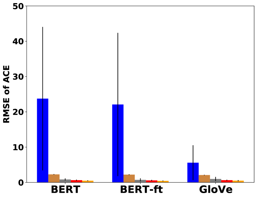
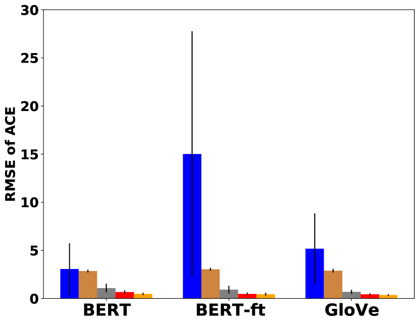
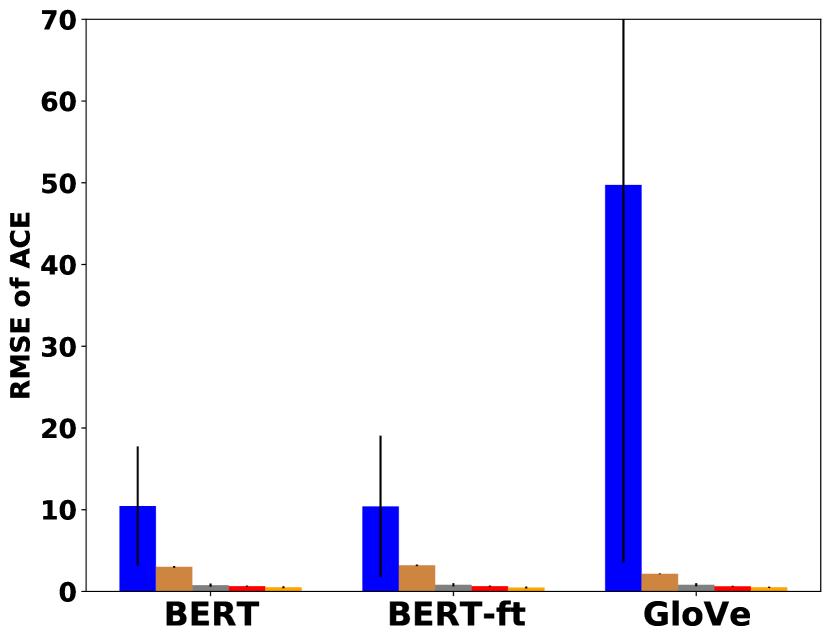
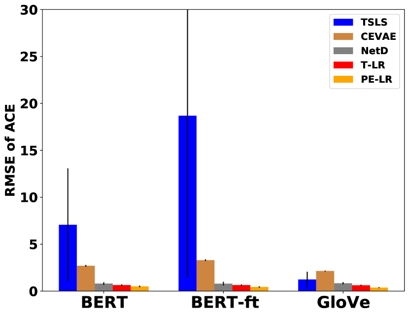
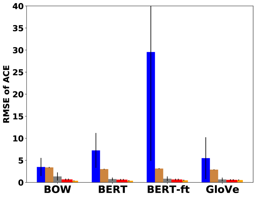
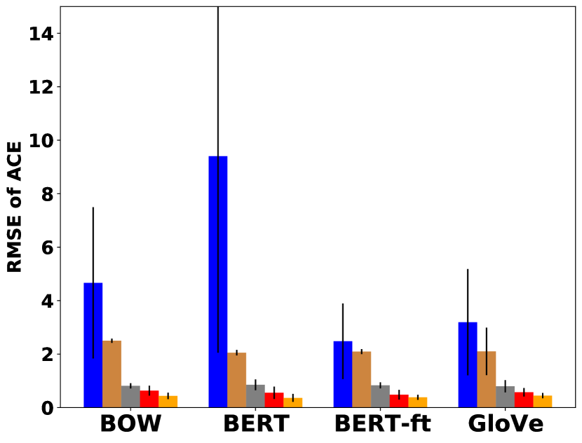
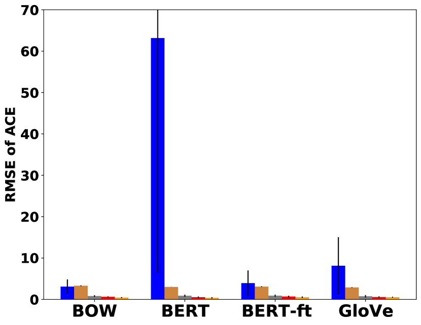
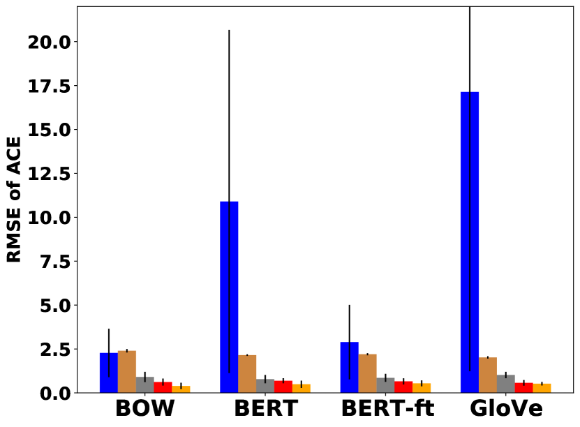
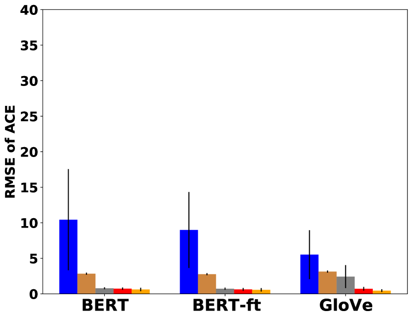
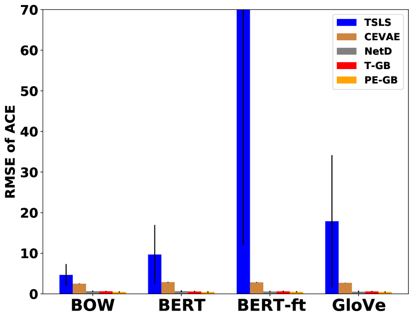
In this experiment, we evaluate the performance of baseline methods using various word embedding techniques. Due to the unavailability of the original text from the BlogCatalog and Flickr datasets, we present the results exclusively for the SAH and Hateful Users datasets. As depicted in Fig. 3, our observations consistently align with those obtained using the BoW method. It is evident that TSLS exhibits the highest levels of bias and variance when estimating contagion effects across different embedding techniques for both datasets with different unobserved confounding coefficients. However, while Netd outperforms both TSLS and CAVAE, it doesn’t quite reach the level of effectiveness demonstrated by our proposed method, PE-GB.

Figure 4. RMSE of ACE in SAH (left) and Hateful Users dataset (right), considering network data and utilizing the max() activation function, with $\beta_{u}\sim\mathcal{N}(0,3)$.

(a) SAH

(b) Hateful Users

(c) BlogCatalog

(d) Flickr

Figure 5. RMSE of ACE in ProEmb with varying embedding vector dimensions in four datasets and $\beta_{u}\sim\mathcal{N}(0,3)$ employing max() activation function. The x-axis represents different types of base-learners used in the counterfactual component of ProEmb.

Comparison between ProEmb variants.

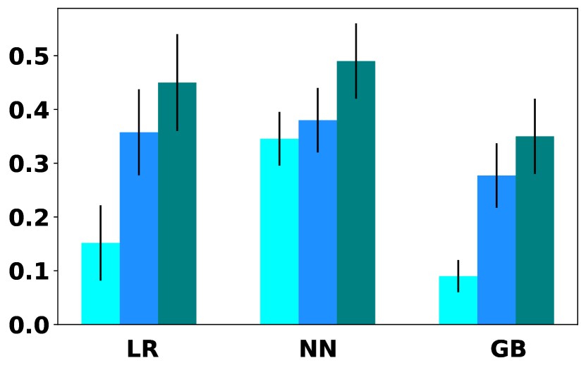
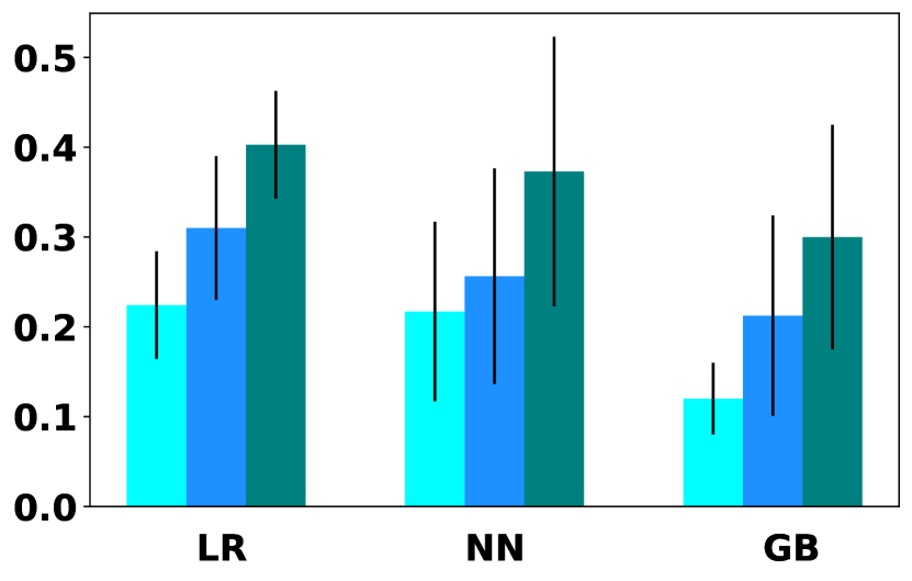
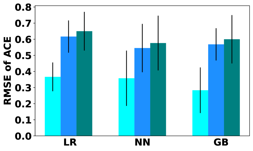
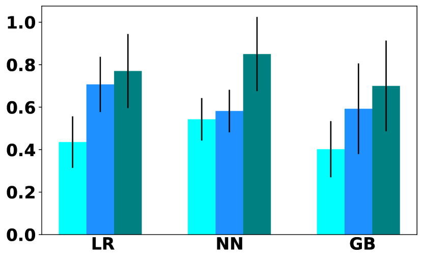
We compare the RMSE of estimated contagion effects using ProEmb and the best-performing baseline, T-Learner, with different base-learners. As Fig. 4 shows, PE-LR and PE-GB outperform other methods in both datasets. Results show that BoW is a more effective feature representation method. One possible explanation is that the topic distribution is derived from BoW vectors, which could serve as a more suitable representation of the latent topics. The RMSE for PE is consistently lower for different base-learners and different features even if they do not always appear to be statistically significant due to overlapping variance. Results across datasets show that PE-GB obtains better performance compared to other variants in most cases.

Sensitivity to the dimension of the embedding

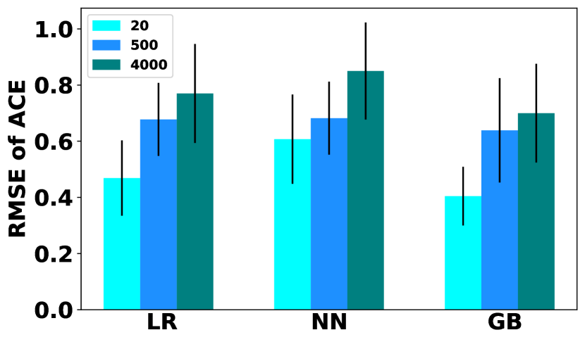
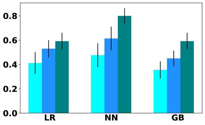
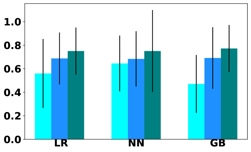
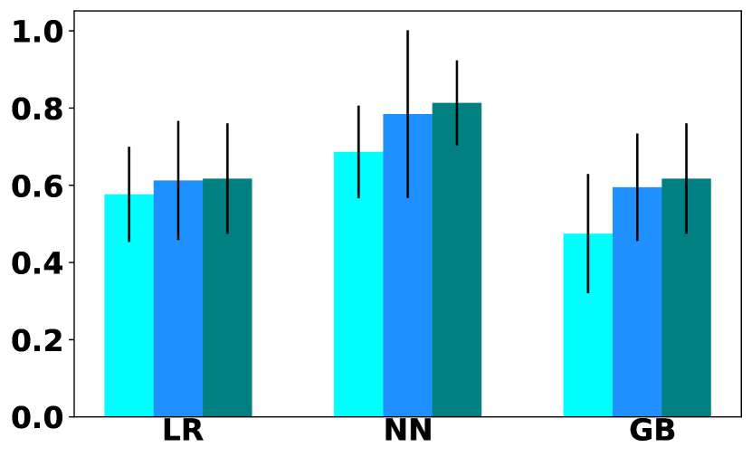
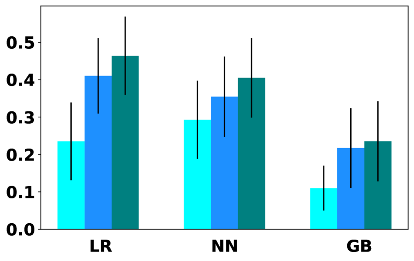
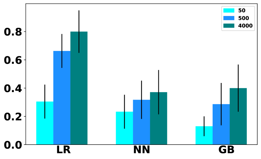
To investigate the impact of the embedding vector dimension on the estimation error of ProEmb variants, we train the ProEmb models with BoW features and different numbers of embedding dimensions from 20 to 4000. Due to the dimensionality and the superior performance of various methods when using BoW feature representation, we employ BoW feature representation in this experiment. As the number of dimensions increases (Fig. 5), the estimation error also increases for all ProEmb variants, with PE-GB achieving the lowest error among all ProEmb variants. The results are consistent across different datasets, with network and dyads ego-network, and when utilizing mean() activation functions, as shown in the Appendix (Fig. 8 and Fig. 11).

Real world demonstration

One of the main challenges in social studies is measuring the effect of friends on their peers and the strength of such effects in different domains. As a demonstration of the applicability of our approach to detecting contagion effects in real-world scenarios, we analyze two datasets: 1) French Election, and 2) Peer Smoking. French Election is a Twitter dataset about the 2017 French presidential election (Burghardt et al., 2023). This dataset comprises of 5.3M tweets related to the election, encompassing attitudes, concerns, and emotions expressed in each tweet. Our objective is to measure the extent to which a friend’s tweet with a specific emotion or attitude influences a user’s decision to post a tweet with the same emotion or attitude. We consider four different outcomes in our analysis: 1) vote against which represents the author’s attitude toward voting against a candidate, 2) anger emotion, 3) love emotion, and 4) religious concern. The preprocessing details about this dataset are available in the Appendix. Overall, we find:

• Friends’ tweets about voting against a candidate have a small negative effect, meaning that they are less likely to tweet about it themselves ($\hat{\theta}_{PE-GB}=-0.013$, p-value=0.001).

• Our method does not reveal a significant contagion effect between users regarding concerns related to religion ($\hat{\theta}_{PE-GB}=-0.002$, p-value = 0) or love emotion ($\hat{\theta}_{PE-GB}=0.007$, p-value=0.019).

• The anger emotions expressed by peers in their tweets have a small negative impact on the emotional tone of users who retweet those posts, leading to a tendency for opposite emotions to be reflected in their retweets ($\hat{\theta}_{PE-GB}=-0.016$, p-value=0).

The Peer Smoking dataset comprises 1,263 9th and 10th graders from 16 high schools in the Chicago area, observed across three distinct waves (Mermelstein et al., 2009). Our primary objective with this dataset is to assess the influence of peer smoking behaviors during Wave I on an individual’s smoking habits during Wave II. We filter the dataset for youth who do not smoke cigarettes in Wave I. We investigate two scenarios: 1) to what extent does an individual’s boyfriend or girlfriend’s smoking behavior affect their own smoking habits?, and 2) How does the smoking behavior of the group of friends an individual hang out with influence their own smoking habits? We examine cigarette smoking habits as outcomes. In the first scenario, we have 14 features for the individual and 14 features for their neighbors. In the second scenario, there are 16 features for the individual and 13 features for their neighbors. To prepare the dataset for analysis, we apply one-hot encoding to convert categorical features into numerical representations. In the first scenario, this results in 51 features for the central node and 84 features for their neighbors. In the second scenario, the individual is characterized by 57 features, while their neighbors have 78 features each. In summary, our findings reveal the following:

• The cigarette smoking habits of boyfriends or girlfriends have a positive effect on the individual’s cigarette smoking behavior ($\hat{\theta}_{PE-GB}=0.112$, p-value= 0.0005). TSLS estimates a similar contagion effect in this scenario; however, it lacks statistical significance ($\hat{\theta}_{TSLS}=0.167$, p-value= 0.366).

• The cigarette smoking habits of the individual’s circle of close friends, have a lower but also positive effect on the cigarette behavior of the individual ($\hat{\theta}_{PE-GB}=0.061$, P-value=0.0001). While TSLS identifies a somewhat stronger contagion effect, this effect is not statistically significant ($\hat{\theta}_{TSLS}=0.127$, p-value= 0.408).

Conclusion

In this paper, we introduce the Proximal Embeddings (ProEmb) framework for increasing the accuracy of contagion effect estimation in observational network data affected by latent homophily and selection bias. Our framework comprises three key components: 1) embedding learning, which utilizes Variational Autoencoders to map high-dimensional proxies to low-dimensional representations and capture latent homophily, 2) representation balancing, which leverages adversarial networks to address the representation mismatch between treatment groups’ proxy representations, and 3) counterfactual learning, which employs meta-learners to estimate counterfactual outcomes. Our results demonstrate the superiority of the ProEmb framework compared to the baselines in reducing the contagion effect estimation error. We observe that using our embedding framework with Bag-of-words as the input representation yields better results compared to off-the-shelf word embedding methods. A potential future direction is developing a framework to account for multi-hop contagion effects in observational data with unobserved confounders.

Appendix A Appendix

Experiments

Datasets

Hateful Users dataset is a sample of Twitter’s retweet graph in which users are annotated as hateful or non-hateful (Ribeiro et al., 2018). In this dataset, we are interested in measuring the causal effect of 5,000 users’ hatefulness on the time their peers spend on the Twitter application/website. We extend this dataset by synthetically generating 1) connections representing user $v_{i}$ retweeting user $v_{j}$’s tweet, 2) the outcome of each node at time $t-1$, indicating the hatefulness of the user, and 3) the outcome of each node at time $t$, indicating the amount of time the individual spends on the Twitter application/website.
Stay-at-Home (SAH) dataset comprises $30,000$ tweets U.S.-based English tweets reflecting users’ attitudes toward stay-at-home orders during the COVID-19 pandemic (Fatemi et al., 2022). Our objective is to investigate the causal effect of having friends who follow social distancing orders on the user’s health. We augment the SAH dataset by synthetically generating: 1) connections indicating that user $v_{i}$ retweeted user $v_{j}$’s tweets, 2) the outcome of each node at time $t-1$, representing the stance of the tweet toward stay-at-home mandates, and 3) the outcome of each node at time $t$, indicating the level of user’s health.
BlogCatalog dataset comprises communities of bloggers actively contributing content within the online BlogCatalog community. The dataset’s features are constructed as bag-of-words representations, capturing the keywords found within bloggers’ personal descriptions. The connections within the dataset symbolize the relationships of friendship and interaction between pairs of bloggers.
French Election dataset contains 5.3M tweets related to the election. We begin by filtering this dataset to include only tweets and retweets that were posted before the second election date (May 2023), resulting in 4.2M tweets. Then, we construct the retweet network containing 3.1M connections. Following this, we filter the dataset for tweets from users who tweeted at least one tweet after retweeting a tweet. This process yields a total of 13k users with 190k tweets. Since a user may have multiple retweets, we consider the average of each user’s tweets’ Bag of Words (BoW) representation, which has a vector size of 7,573, as the NCO proxy. Additionally, we calculate the average of each user’s retweet embeddings and use them as the NCE proxy. We employ the BoW representation because our approach yields the lowest estimation error when it is utilized. We use the mean() activation function in this experiment. We report the estimation of the contagion effect using PE-GB because it achieves the best performance in almost all datasets.

(a) SAH, $\beta_{u}\sim\mathcal{N}(0,3)$

(b) SAH, $\beta_{u}\sim\mathcal{N}(5,2)$

(c) Hateful, $\beta_{u}\sim\mathcal{N}(0,3)$

(d) Hateful, $\beta_{u}\sim\mathcal{N}(5,2)$

Figure 6. Comparison of RMSE of ACE using various baseline methods in dyadic data. Error bars represent the standard deviation of the estimated effects.

Figure 7. RMSE of ACE in SAH (left) and Hateful Users dataset (right) using dyadic data and $\beta_{u}\sim\mathcal{N}(0,3)$.

(a) SAH, $\beta_{u}\sim\mathcal{N}(0,3)$

(b) SAH, $\beta_{u}\sim\mathcal{N}(5,2)$

(c) Hateful, $\beta_{u}\sim\mathcal{N}(0,3)$

(d) Hateful, $\beta_{u}\sim\mathcal{N}(5,2)$

Figure 8. RMSE of ACE in ProEmb with varying embedding vector dimensions in SAH and Hateful Users dataset with dyadic data. The x-axis represents different types of base-learners used in the counterfactual component of the ProEmb framework.

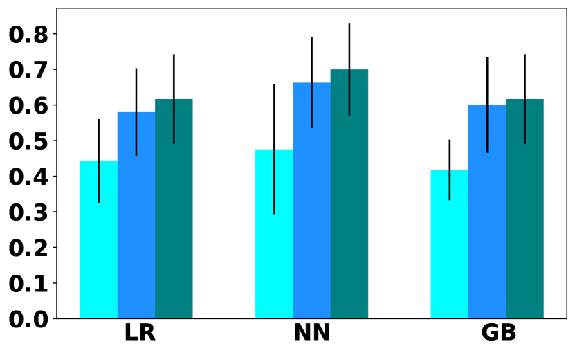
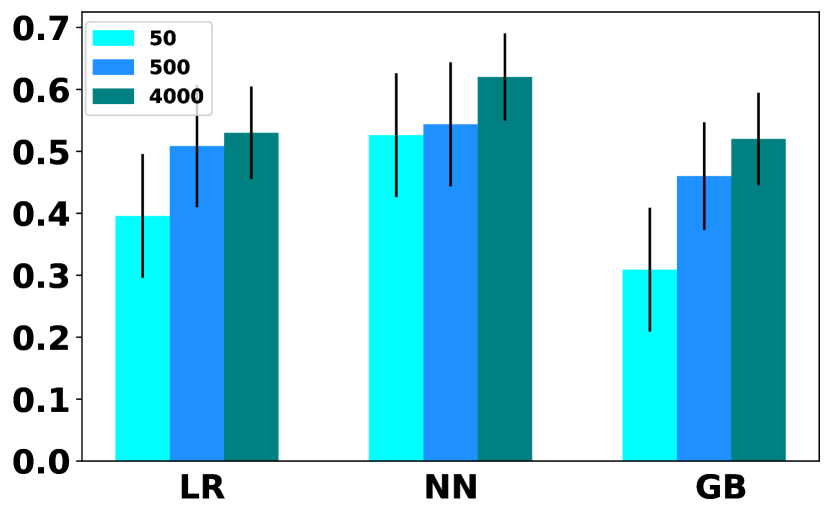
Hyperparameter tuning

To train the VAEs, discriminators, and MLP models, we conduct a hyperparameter search for the learning rate and the number of epochs. The learning rate is searched within the set $\{0.1,0.01,0.001,0.0001\}$, while the number of epochs is searched within $\{10,30,50,70,100\}$. The best results are achieved with a learning rate of 0.001 and 50 epochs for both models. For the VAEs, we search the number of hidden units of the hidden layers in $\{100,200,300\}$ and the number of encoder and decoder layers in ${1,2,3,4}$. We select a network with 100 hidden nodes, a 3-layer encoder, and a 3-layer decoder with a ReLU activation function. In the discriminator component, after hyperparameter search, we determine that four hidden layers, with linear activation functions, produce the best performance. The output layer utilizes a Sigmoid function. Regarding the MLP, we search for the number of hidden units and the number of fully connected layers. Ultimately, we train an MLP model with two fully connected layers, each containing 125 hidden units. In BERT-ft, We use the $AdamW$ optimizer with a learning rate of $2e-5$, max-seq-length of $128$, and batch sizes of $32$.

(a) SAH, $\beta_{u}\sim\mathcal{N}(0,3)$

(b) Hateful Users, $\beta_{u}\sim\mathcal{N}(0,3)$

Figure 9. RMSE of ACE in SAH (left) and Hateful Users dataset (right) using network data employing mean() activation function and $\beta_{u}\sim\mathcal{N}(0,3)$.

Figure 10. RMSE of ACE in SAH (left) and Hateful Users dataset (right) using network data deploying mean() activation function and $\beta_{u}\sim\mathcal{N}(0,3)$.

(a) SAH

(b) Hateful Users

(c) BlogCatalog

(d) Flickr

Figure 11. RMSE of ACE in ProEmb with varying embedding vector dimensions in four datasets and $\beta_{u}\sim\mathcal{N}(0,3)$ employing mean() activation function. The x-axis represents different types of base-learners used in the counterfactual component of the ProEmb framework.

Results

Contagion effect estimation evaluation for dyadic data

In this section, we present the results of a comparative analysis among various methods used to estimate peer contagion effects in the SAH and Hateful Users datasets, based on dyad data with distinct $\beta_{u}$ vectors. These findings align consistently with the results from the network data. As depicted in Figure 6, TSLS exhibits the highest estimation error when compared to other baseline methods, whereas T-LR demonstrates more favorable performance. The results illustrated in Fig. 10 further show that PE-LR and PE-G methods outperform other approaches in terms of reducing contagion effect estimation errors.

In terms of sensitivity to the dimension of the embedding, as Fig. 8 shows, by increasing the number of embedding dimensions from 20 to 4,000 in SAH and from 50 to 4000 in the Hateful Users dataset, the estimation error of the ProEmb method increases. This finding confirms the necessity of applying dimension-reduction techniques when dealing with high-dimensional data.

Contagion effect estimation evaluation for network data

In this experiment, we use mean() activation function for h(). Figure 9 demonstrates that TSLS receives the highest bias and variance in both SAH and Hateful Users datasets. Similar to experiments with max() activation function, we observe that our framework, PE-GB achieves the best performance with different feature representation techniques. Regarding sensitivity to the dimension of the embedding, we obtain consistent results with data on dyads and network data with max() activation function. In all datasets, by increasing the dimension of the emebeddings, the estimation error of the method increases (Fig. 11).

References

- (1)
- Abadie and Imbens (2006) Alberto Abadie and Guido W Imbens. 2006. Large sample properties of matching estimators for average treatment effects. econometrica 74, 1 (2006), 235–267.
- Angrist and Imbens (1995) Joshua D Angrist and Guido W Imbens. 1995. Two-stage least squares estimation of average causal effects in models with variable treatment intensity. Journal of the American statistical Association 90, 430 (1995), 431–442.
- Assaad et al. (2021) Serge Assaad, Shuxi Zeng, Chenyang Tao, Shounak Datta, Nikhil Mehta, Ricardo Henao, Fan Li, and Lawrence Carin. 2021. Counterfactual representation learning with balancing weights. In International Conference on Artificial Intelligence and Statistics. PMLR, 1972–1980.
- Bernardo et al. (2003) JM Bernardo, MJ Bayarri, JO Berger, AP Dawid, D Heckerman, AFM Smith, and M West. 2003. Bayesian factor regression models in the “large p, small n” paradigm. Bayesian statistics 7 (2003), 733–742.
- Blei et al. (2003) David M. Blei, Andrew Y. Ng, and Michael I. Jordan. 2003. Latent Dirichlet Allocation. Journal of Machine Learning Research 3, Jan (2003), 993–1022. https://www.jmlr.org/papers/v3/blei03a
- Bramoullé et al. (2009) Yann Bramoullé, Habiba Djebbari, and Bernard Fortin. 2009. Identification of peer effects through social networks. Journal of econometrics 150, 1 (2009), 41–55.
- Burghardt et al. (2023) Keith Burghardt, Ashwin Rao, Siyi Guo, Zihao He, Georgios Chochlakis, Baruah Sabyasachee, Andrew Rojecki, Shri Narayanan, and Kristina Lerman. 2023. Socio-Linguistic Characteristics of Coordinated Inauthentic Accounts. arXiv preprint arXiv:2305.11867 (2023).
- Chao and Swanson (2005) John C Chao and Norman R Swanson. 2005. Consistent estimation with a large number of weak instruments. Econometrica 73, 5 (2005), 1673–1692.
- Christakis and Fowler (2007) Nicholas A Christakis and James H Fowler. 2007. The spread of obesity in a large social network over 32 years. New England journal of medicine 357, 4 (2007), 370–379.
- Christakis and Fowler (2008) Nicholas A Christakis and James H Fowler. 2008. The collective dynamics of smoking in a large social network. New England journal of medicine 358, 21 (2008), 2249–2258.
- Cristali and Veitch (2021) Irina Cristali and Victor Veitch. 2021. Using Embeddings to Estimate Peer Influence on Social Networks. In NeurIPS 2021.
- De Luna et al. (2011) Xavier De Luna, Ingeborg Waernbaum, and Thomas S Richardson. 2011. Covariate selection for the nonparametric estimation of an average treatment effect. Biometrika 98, 4 (2011), 861–875.
- Deaner (2021) Ben Deaner. 2021. Many Proxy Controls. arXiv preprint arXiv:2110.03973 (2021).
- Devlin et al. (2019) Jacob Devlin, Ming-Wei Chang, Kenton Lee, and Kristina Toutanova. 2019. BERT: Pre-training of Deep Bidirectional Transformers for Language Understanding. In Proceedings of the 2019 Conference of the North American Chapter of the Association for Computational Linguistics: Human Language Technologies, Volume 1 (Long and Short Papers).
- Eckles et al. (2016) D. Eckles, R. Kizilcec, and E. Bakshy. 2016. Estimating peer effects in networks with peer encouragement designs. PNAS (2016).
- Egami and Tchetgen (2021) Naoki Egami and Eric J Tchetgen Tchetgen. 2021. Identification and Estimation of Causal Peer Effects Using Double Negative Controls for Unmeasured Network Confounding. arXiv preprint arXiv:2109.01933 (2021).
- Fatemi et al. (2022) Zahra Fatemi, Abari Bhattacharya, Andrew Wentzel, Vipul Dhariwal, Lauren Levine, Andrew Rojecki, G Elisabeta Marai, Barbara Di Eugenio, and Elena Zheleva. 2022. Understanding Stay-at-home Attitudes through Framing Analysis of Tweets. IEEE International Conference on Data Science and Advanced Analytics (DSAA) (2022).
- Fowler and Christakis (2008) James H Fowler and Nicholas A Christakis. 2008. Estimating peer effects on health in social networks: a response to Cohen-Cole and Fletcher; Trogdon, Nonnemaker, Pais. Journal of health economics 27, 5 (2008), 1400.
- Goodfellow et al. (2014) Ian Goodfellow, Jean Pouget-Abadie, Mehdi Mirza, Bing Xu, David Warde-Farley, Sherjil Ozair, Aaron Courville, and Yoshua Bengio. 2014. Generative Adversarial Nets. In Advances in Neural Information Processing Systems, Z. Ghahramani, M. Welling, C. Cortes, N. Lawrence, and K.Q. Weinberger (Eds.), Vol. 27. Curran Associates, Inc. https://proceedings.neurips.cc/paper˙files/paper/2014/file/5ca3e9b122f61f8f06494c97b1afccf3-Paper.pdf
- Grari et al. (2022) Vincent Grari, Sylvain Lamprier, and Marcin Detyniecki. 2022. Fairness without the Sensitive Attribute via Causal Variational Autoencoder. In Thirty-First International Joint Conference on Artificial Intelligence IJCAI-22. International Joint Conferences on Artificial Intelligence Organization, 696–702.
- Gregor et al. (2015) Karol Gregor, Ivo Danihelka, Alex Graves, Danilo Rezende, and Daan Wierstra. 2015. Draw: A recurrent neural network for image generation. In International conference on machine learning. PMLR, 1462–1471.
- Guo et al. (2020) Ruocheng Guo, Jundong Li, and Huan Liu. 2020. Learning individual causal effects from networked observational data. In WSDM. 232–240.
- Hansen et al. (2008) Christian Hansen, Jerry Hausman, and Whitney Newey. 2008. Estimation with many instrumental variables. Journal of Business & Economic Statistics 26, 4 (2008), 398–422.
- Hassanpour and Greiner (2019) Negar Hassanpour and Russell Greiner. 2019. CounterFactual Regression with Importance Sampling Weights.. In IJCAI. 5880–5887.
- Im et al. (2021) Daniel Jiwoong Im, Kyunghyun Cho, and Narges Razavian. 2021. Causal effect variational autoencoder with uniform treatment. arXiv preprint arXiv:2111.08656 (2021).
- Jiang and Sun (2022a) Song Jiang and Yizhou Sun. 2022a. Estimating Causal Effects on Networked Observational Data via Representation Learning. In Proceedings of the 31st ACM International Conference on Information & Knowledge Management. 852–861.
- Jiang and Sun (2022b) Song Jiang and Yizhou Sun. 2022b. Estimating Causal Effects on Networked Observational Data via Representation Learning. In Proceedings of the 31st ACM International Conference on Information & Knowledge Management. 852–861.
- Jimenez Rezende et al. (2016) Danilo Jimenez Rezende, SM Eslami, Shakir Mohamed, Peter Battaglia, Max Jaderberg, and Nicolas Heess. 2016. Unsupervised learning of 3d structure from images. Advances in neural information processing systems 29 (2016).
- Johansson et al. (2016) Fredrik D. Johansson, Uri Shalit, and David Sontag. 2016. Learning Representations for Counterfactual Inference. In ICML- Volume 48 (New York, NY, USA) (ICML’16). JMLR.org, 3020–3029.
- Kim et al. (2021) Hyemi Kim, Seungjae Shin, JoonHo Jang, Kyungwoo Song, Weonyoung Joo, Wanmo Kang, and Il-Chul Moon. 2021. Counterfactual fairness with disentangled causal effect variational autoencoder. In Proceedings of the AAAI Conference on Artificial Intelligence, Vol. 35. 8128–8136.
- Kingma and Welling (2014) Diederik P Kingma and Max Welling. 2014. Auto-Encoding Variational Bayes. stat 1050 (2014), 1.
- Krauth (2005) Brian V Krauth. 2005. Peer effects and selection effects on smoking among Canadian youth. Canadian Journal of Economics/Revue canadienne d’économique 38, 3 (2005), 735–757.
- Kullback and Leibler (1951) Solomon Kullback and Richard A Leibler. 1951. On information and sufficiency. The annals of mathematical statistics 22, 1 (1951), 79–86.
- Künzel et al. (2019) Sören R Künzel, Jasjeet S Sekhon, Peter J Bickel, and Bin Yu. 2019. Metalearners for estimating heterogeneous treatment effects using machine learning. Proceedings of the national academy of sciences 116, 10 (2019), 4156–4165.
- Lauritzen and Richardson (2002) Steffen L Lauritzen and Thomas S Richardson. 2002. Chain graph models and their causal interpretations. Journal of the Royal Statistical Society: Series B (Statistical Methodology) 64, 3 (2002), 321–348.
- Li and Fu (2017) Sheng Li and Yun Fu. 2017. Matching on balanced nonlinear representations for treatment effects estimation. Advances in Neural Information Processing Systems 30 (2017).
- Louizos et al. (2017) Christos Louizos, Uri Shalit, Joris M Mooij, David Sontag, Richard Zemel, and Max Welling. 2017. Causal effect inference with deep latent-variable models. Advances in neural information processing systems 30 (2017).
- Manski (1993) Charles F Manski. 1993. Identification of endogenous social effects: The reflection problem. The review of economic studies 60, 3 (1993), 531–542.
- Mermelstein et al. (2009) Robin J Mermelstein, Peter J Colvin, and Sven D Klingemann. 2009. Dating and changes in adolescent cigarette smoking: does partner smoking behavior matter? Nicotine & Tobacco Research 11, 10 (2009), 1226–1230.
- Mescheder et al. (2017) Lars Mescheder, Sebastian Nowozin, and Andreas Geiger. 2017. Adversarial variational bayes: Unifying variational autoencoders and generative adversarial networks. In International conference on machine learning. PMLR, 2391–2400.
- Miao et al. (2018) Wang Miao, Zhi Geng, Eric J Tchetgen Tchetgen, et al. 2018. Identifying causal effects with proxy variables of an unmeasured confounder. Biometrika 105, 4 (2018), 987–993.
- Ogburn et al. (2017) Elizabeth L Ogburn, Oleg Sofrygin, Ivan Diaz, and Mark J Van Der Laan. 2017. Causal inference for social network data. arXiv preprint arXiv:1705.08527 (2017).
- Ogburn and VanderWeele (2014) Elizabeth L Ogburn and Tyler J VanderWeele. 2014. Causal diagrams for interference. Statistical science 29, 4 (2014), 559–578.
- Pearl (2009) Judea Pearl. 2009. Causality. Cambridge Univ Press.
- Pennington et al. (2014) Jeffrey Pennington, Richard Socher, and Christopher D. Manning. 2014. GloVe: Global Vectors for Word Representation. In EMNLP. 1532–1543. http://www.aclweb.org/anthology/D14-1162
- Piva et al. (2021) Gabriel G Piva, Fabiano L Ribeiro, and Angélica S Mata. 2021. Networks with growth and preferential attachment: modelling and applications. Journal of Complex Networks 9, 1 (2021), cnab008.
- Portillo et al. (2020) Stephen KN Portillo, John K Parejko, Jorge R Vergara, and Andrew J Connolly. 2020. Dimensionality reduction of SDSS spectra with variational autoencoders. The Astronomical Journal 160, 1 (2020), 45.
- Pu et al. (2016) Yunchen Pu, Zhe Gan, Ricardo Henao, Xin Yuan, Chunyuan Li, Andrew Stevens, and Lawrence Carin. 2016. Variational autoencoder for deep learning of images, labels and captions. Advances in neural information processing systems 29 (2016).
- Rezende et al. (2014) Danilo Jimenez Rezende, Shakir Mohamed, and Daan Wierstra. 2014. Stochastic backpropagation and approximate inference in deep generative models. In International conference on machine learning. PMLR, 1278–1286.
- Ribeiro et al. (2018) Manoel Horta Ribeiro, Pedro H Calais, Yuri A Santos, Virgílio AF Almeida, and Wagner Meira Jr. 2018. Characterizing and detecting hateful users on twitter. In ICWSM.
- Rosenbaum and Rubin (1983) Paul R Rosenbaum and Donald B Rubin. 1983. The central role of the propensity score in observational studies for causal effects. Biometrika 70, 1 (1983), 41–55.
- Shalit et al. (2017) Uri Shalit, Fredrik D Johansson, and David Sontag. 2017. Estimating individual treatment effect: generalization bounds and algorithms. In International Conference on Machine Learning. PMLR, 3076–3085.
- Shalizi and McFowland III (2016) Cosma Rohilla Shalizi and Edward McFowland III. 2016. Estimating causal peer influence in homophilous social networks by inferring latent locations. arXiv preprint arXiv:1607.06565 (2016).
- Shalizi and Thomas (2011) Cosma Rohilla Shalizi and Andrew C Thomas. 2011. Homophily and contagion are generically confounded in observational social network studies. Sociological methods & research 40, 2 (2011), 211–239.
- Stuart (2010) Elizabeth A Stuart. 2010. Matching methods for causal inference: A review and a look forward. Statistical science 25, 1 (2010), 1.
- Tchetgen et al. (2020) Eric J Tchetgen Tchetgen, Andrew Ying, Yifan Cui, Xu Shi, and Wang Miao. 2020. An introduction to proximal causal learning. arXiv preprint arXiv:2009.10982 (2020).
- Torres et al. (2018) Russell Torres, Natalie Gerhart, and Arash Negahban. 2018. Epistemology in the Era of Fake News: An Exploration of Information Verification Behaviors among Social Networking Site Users. SIGMIS Database 49, 3 (jul 2018), 78–97. https://doi.org/10.1145/3242734.3242740
- VanderWeele and An (2013) Tyler J VanderWeele and Weihua An. 2013. Social networks and causal inference. Handbook of causal analysis for social research (2013), 353–374.
- Veitch et al. (2019) Victor Veitch, Yixin Wang, and David Blei. 2019. Using embeddings to correct for unobserved confounding in networks. Neurips 32 (2019).
- Wang et al. (2014) Wei Wang, Yan Huang, Yizhou Wang, and Liang Wang. 2014. Generalized autoencoder: A neural network framework for dimensionality reduction. In CVPR workshops. 490–497.