An Inexact Conditional Gradient Method for Constrained Bilevel Optimization

Abstract

Bilevel optimization is an important class of optimization problems where one optimization problem is nested within another. This framework is widely used in machine learning problems, including meta-learning, data hyper-cleaning, and matrix completion with denoising. In this paper, we focus on a bilevel optimization problem with a strongly convex lower-level problem and a smooth upper-level objective function over a compact and convex constraint set. Several methods have been developed for tackling unconstrained bilevel optimization problems, but there is limited work on methods for the constrained setting. In fact, for those methods that can handle constrained problems, either the convergence rate is slow or the computational cost per iteration is expensive. To address this issue, in this paper, we introduce a novel single-loop projection-free method using a nested approximation technique. Our proposed method has an improved per-iteration complexity, surpassing existing methods, and achieves optimal convergence rate guarantees matching the best-known complexity of projection-free algorithms for solving convex constrained single-level optimization problems. In particular, when the upper-level objective function is convex, our method requires $\tilde{\mathcal{O}}(\epsilon^{-1})$ iterations to find an $\epsilon$-optimal solution. Moreover, when the upper-level objective function is non-convex the complexity of our method is $\mathcal{O}(\epsilon^{-2})$ to find an $\epsilon$-stationary point. We also present numerical experiments to showcase the superior performance of our method compared with state-of-the-art methods.

1 Introduction

Many learning and inference problems take a hierarchical form, where one optimization problem is nested within another. Bilevel optimization is often used to model problems of this kind with two levels of hierarchy. In this paper, we consider the bilevel optimization problem of the following form

$$\min_{\mathbf{x}\in\mathcal{X}}~{}\ell(\mathbf{x}):=f(\mathbf{x},\mathbf{y}^{*}(\mathbf{x}))\qquad\hbox{s.t.}\quad\mathbf{y}^{*}(\mathbf{x})\in\operatorname*{\arg\!\min}_{\mathbf{y}\in\mathbb{R}^{m}}~{}g(\mathbf{x},\mathbf{y}).$$ (1)

where $n,m\geq 1$ are integers; $\mathcal{X}\subset\mathbb{R}^{n}$ is a compact and convex set, $f:\mathcal{X}\times\mathbb{R}^{m}\to\mathbb{R}$ and $g:\mathcal{X}\times\mathbb{R}^{m}\to\mathbb{R}$ are continuously differentiable functions with respect to (w.r.t.) $\mathbf{x}$ and $\mathbf{y}$ on an open set containing $\mathcal{X}$ and $\mathbb{R}^{m}$, respectively. Problem 1 involves two optimization problems following a two-level structure. The outer objective $f(\mathbf{x},\mathbf{y}^{*}(\mathbf{x}))$ depends on $\mathbf{x}$ both directly and also indirectly through $\mathbf{y}^{*}(\mathbf{x})$ which is a solution of the lower-level problem of minimizing another function $g$ parameterized by $\mathbf{x}$. Throughout the paper, we assume that $g(\mathbf{x},\mathbf{y})$ is strongly convex in $\mathbf{y}$, hence, $\mathbf{y}^{*}(\mathbf{x})$ is uniquely well-defined for all $\mathbf{x}\in\mathcal{X}$. The application of (1) arises in a number of machine learning problems, such as meta-learning [RFKL19], continual learning [BMK20], reinforcement learning [KT99], hyper-parameter optimization[FFSGP18a, Ped16], and data hyper-cleaning [SCHB19].

Several methods have been proposed to solve the general form of the bilevel optimization problems mentioned in (1). For instance, using the optimality conditions of the lower-level problem, the works in [HJS92, SLZ05, Moo10] transformed the bilevel problem into a single-level constrained problem. However, such an approach includes two major challenges: $(i)$ The reduced problem will have too many constraints when the inner problem is large-scale; $(ii)$ Unless the lower-level function $g$ has a specific structure, such as a quadratic form, the optimality condition of the lower-level problem introduces nonconvexity into the feasible set of the reduced problem. Recently, more efficient gradient-based bilevel optimization algorithms have been proposed, which can be broadly divided into the approximate implicit differentiation (AID) based approach [Ped16, GFCACG16, Dom12, LXFZYPUZ18, GW18, LVD20] and the iterative differentiation (ITD) based approach [SCHB19, MDA15, FFSGP18, GFPS20]. Nevertheless, with the exception of a few recent attempts, most of the existing studies have primarily focused on analyzing the asymptotic convergence leaving room for the development of novel algorithms that come with guaranteed convergence rates.

Moreover, in most prior studies the constraint set $\mathcal{X}$ is assumed to be $\mathcal{X}=\mathbb{R}^{n}$ to create a simpler unconstrained upper optimization problem. Nonetheless, in several applications, such as meta-learning [FFSGP18a], personalized federated learning[FMO20], and core sets selection [BMK20], $\mathcal{X}$ is a strict subset of $\mathbb{R}^{n}$. Using projected gradient methods is a common approach when dealing with such constraint sets. Despite their widespread use, projected gradient techniques may not always be applicable. The limitations of projection-based techniques led to the development of projection-free algorithms like Frank Wolfe-based methods [FW56]. Instead of tackling a non-linear projection problem, as in the case of $\ell_{1}$-norm or nuclear norm ball restrictions, these Frank Wolfe-based techniques just need to solve a linear minimization problem over $\mathcal{X}$ with lower computational complexity.

Table 1: Summary of algorithms for solving general bilevel optimization with a strongly convex lower-level objective function. The abbreviations “C”, “NC”, “PO”, “LMO” stand for “convex”, “non-convex”, “projection oracle”, and “linear minimization oracle” respectively and $\kappa_{g}\triangleq L_{g}/\mu_{g}$. For the algorithms with $\mathcal{O}(m^{2}\log(K))$ per-iteration dependence, the Hessian inverse can be computed via multiple rounds of matrix-vector products. ^∗ Note that these works focused on convergence rates in the stochastic setting, without addressing the rates in the deterministic setting. As the results did not explicitly provide rates for the deterministic setting, we present the results for the stochastic setting.

	Reference	oracle	function $f$	$\#$ loops	Iteration complexity		Convergence rate
			NC/C				Upper level	Lower level
Unconstrained	SUSTAIN [KZHWWY21]	—–	NC	single loop	$\mathcal{O}(\kappa_{g}m^{2}\log(K))$		$\mathcal{O}(\epsilon^{-1})$
	FSLA [LGH22]	—–	NC	single loop	$\mathcal{O}(m^{2})$		$\mathcal{O}(\epsilon^{-1})$
	F3SA [KKWN23]	—–	NC	single loop	$\mathcal{O}(m)$		$\tilde{\mathcal{O}}(\epsilon^{-\frac{3}{2}})$
	AID-BiO [JYL20]	—–	NC	double loop	$\mathcal{O}(\sqrt{\kappa_{g}}m^{2})$		$\mathcal{O}(\epsilon^{-1})$
Constrained	ABA[GW18]	PO	NC	double loop	$\mathcal{O}(m^{3})$		$\mathcal{O}(\epsilon^{-1})$	$\mathcal{O}(\epsilon^{-\frac{5}{4}})$
			C				$\mathcal{O}(\epsilon^{-\frac{1}{2}})$	$\mathcal{O}(\epsilon^{-\frac{3}{4}})$
	TTSA∗ [HWWY20]	PO	NC	single loop	$\mathcal{O}(\kappa_{g}m^{2}\log(K))$		$\mathcal{O}(\epsilon^{-\frac{5}{2}})$
			C				$\mathcal{O}(\epsilon^{-4})$	$\mathcal{O}(\epsilon^{-2})$
	SBFW∗ [ABTR22]	LMO	NC	single loop	$\mathcal{O}(\kappa_{g}m^{2}\log(K))$		$\mathcal{O}(\epsilon^{-4})$	$\mathcal{O}(\epsilon^{-\frac{5}{2}})$
			C				$\mathcal{O}(\epsilon^{-3})$	$\mathcal{O}(\epsilon^{-\frac{3}{2}})$
	Ours	LMO	NC	single loop	$\mathcal{O}(m^{2})$		$\mathcal{O}(\epsilon^{-2})$
			C				$\tilde{\mathcal{O}}(\epsilon^{-1})$

In the context of bilevel optimization problems, there have been several studies considering constrained settings. However, most existing methods focus on projection-based algorithms, with limited exploration of projection-free alternatives. Moreover, these methods usually suffer from a slow convergence rate or involve a high computational cost per iteration. In particular, the fast convergence guarantees for these methods such as [GW18] is achieved by utilizing the Hessian inverse of the lower-level function which comes at a steep price, with the worst-case computational cost of $\mathcal{O}(m^{3})$ limiting its application. To resolve this issue, a Hessian inverse approximation technique was introduced in [GW18] and used in other studies such as [HWWY20, ABTR22]. This approximation technique introduces a vanishing biased as the number of inner steps (matrix-vector multiplications) increases and its computational complexity scales with the lower-level problem’s condition number. In particular, it has a per-iteration complexity of $\mathcal{O}(\kappa_{g}m^{2}\log(K))$ where $\kappa_{g}$ denotes the condition number of the function $g$.

To overcome these issues, we develop a new inexact projection-free method that achieves optimal convergence rate guarantees for the considered settings while requiring only two matrix-vector products per iteration leading to a complexity of $\mathcal{O}(m^{2})$ per iteration. Next, we state our contributions.

Contributions. In this paper, we consider a class of bilevel optimization problems with a strongly convex lower-level problem and a smooth upper-level objective function over a compact and convex constraint set. This extends the literature, which has primarily focused on unconstrained optimization problems. This paper introduces a novel single-loop projection-free method that overcomes the limitations of existing approaches by offering improved per-iteration complexity and convergence guarantees. Our main idea is to simultaneously keep track of trajectories of lower-level optimal solution as well as a parametric quadratic programming containing Hessian inverse information using a nested approximation. These estimations are calculated using a one-step gradient-type step and are used to estimate the hyper-gradient for a Frank Wolfe-type update. Notably, using this approach our proposed method requires only two matrix-vector products at each iteration which presents a substantial improvement compared to the existing methods. Moreover, our theoretical guarantees for the proposed Inexact Bilevel Conditional Gradient method denoted by IBCG are as follows:

• When the upper-level function $f$ is convex, we show that our IBCG method requires $\tilde{\mathcal{O}}(\epsilon^{-1})$ iterations to find an $\epsilon$-optimal solution.

• When $f$ is non-convex, IBCG requires $\mathcal{O}(\epsilon^{-2})$ iterations to find an $\epsilon$-stationary point.

These results match the best-known complexity of projection-free algorithms for solving convex constrained single-level optimization problems.

Related work. In this section, we review some of the related works in the context of general bilevel optimization in a deterministic/stochastic setting and projection-free algorithms.
The concept of bilevel optimization was initially introduced by Bracken and McGill in 1973 [BM73]. Since then, researchers have proposed several algorithms for solving bilevel optimization problems, with various approaches including but not limited to constraint-based methods [SLZ05, Moo10] and gradient-based methods. In recent years, gradient-based methods for dealing with problem (1) have become increasingly popular including implicit differentiation [Dom12, Ped16, GFCACG16, GW18, JYL21] and iterative differentiation [FFSGP18, MDA15]. There are several single and double loop methods developed for tackling unconstrained bilevel optimization problems in the literature [CSXY22, LGH22, KKWN23, KZHWWY21, JYL20]; however, the number of works focusing on the constrained bilevel optimization problems are limited. On this basis, the seminal work in [GW18] presented an Accelerated Bilevel Approximation (ABA) method which consists of two iterative loops and it is shown that when the upper-level function is non-convex ABA obtains a convergence rate of $\mathcal{O}(\epsilon^{-1})$ and $\mathcal{O}(\epsilon^{-\frac{5}{4}})$ in terms of the upper-level and lower-level objective values respectively. Although their convergence guarantees in both convex and non-convex settings are superior to other similar works, their computational complexity is too expensive as they need to compute the Hessian inverse matrix at each iteration. Built upon the work of [GW18], authors in [HWWY20] proposed a Two-Timescale Stochastic Approximation (TTSA) algorithm which is shown to achieve a complexity of $\mathcal{O}(\epsilon^{-\frac{5}{2}})$ when the upper-level function is non-convex. Results for the convex case are also included in Table 1. It should be noted that these methods require a projection onto set $\mathcal{X}$ at every iteration. In contrast, as our proposed method is a projection-free method, it requires access to a linear solver instead of projection at each iteration, which is suitable for the settings where projection is computationally costly; e.g., when $\mathcal{X}$ is a nuclear-norm ball. In [ABTR22], which is closely related to our work, authors developed a projection-free stochastic optimization algorithm (SBFW) for bilevel optimization problems and it is shown that their method achieves the complexity of $\mathcal{O}(\epsilon^{-4})$ and $\mathcal{O}(\epsilon^{-\frac{5}{2}})$ with respect to the upper and lower-level problem respectively.

We note that most of the work studied bilevel optimization problems in the stochastic setting and did not provide any results for the deterministic setting motivating us to focus on this category of bilevel problems to improve the convergence and computational complexity over existing methods. Some concurrent papers consider the case where the lower-level problem can have multiple minima [LMYZZ20, SJGL22, CXZ23]. As they consider a more general setting that brings more challenges, their theoretical results are also weaker, providing only asymptotic convergence guarantees or slower convergence rates.

2 Preliminaries

2.1 Motivating examples

The applications of bilevel optimization formulation in (1) include many machine learning problems such as matrix completion [YH17], meta-learning [RFKL19], data hyper-cleaning [SCHB19], hyper-parameter optimization [FFSGP18a], etc. Next, we describe two examples in details.

Matrix Completion with Denoising: Consider the matrix completion problem where the goal is to recover missing items from imperfect and noisy observations of a random subset of the matrix’s entries. Generally, with noiseless data, the data matrix can be represented as a low-rank matrix, which justifies the use of the nuclear norm constraint. In numerous applications, such as image processing and collaborative filtering, the observations are noisy, and solving the matrix completion problem using only the nuclear norm restrictions can result in sub-optimal performance [MD21, YH17]. One approach to include the denoising step in the matrix completion formulation is to formulate the problem as a bilevel optimization problem [ABTR22]. This problem can be expressed as follows:

$$\min_{\|\mathbf{X}\|_{*}\leq\alpha}~{}\frac{1}{\left|\Omega_{1}\right|}\sum_{(i,j)\in\Omega_{1}}(\mathbf{X}_{i,j}-\mathbf{Y}_{i,j})^{2}$$

$$\;\,\hbox{s.t.}\quad\mathbf{Y}\in\operatorname*{\arg\!\min}_{\mathbf{V}}~{}\Big{\{}\frac{1}{\left|\Omega_{2}\right|}\sum_{(i,j)\in\Omega_{2}}(\mathbf{V}_{i,j}-\mathbf{M}_{i,j})^{2}+\lambda_{1}\mathcal{R}(\mathbf{V})+\lambda_{2}\|\mathbf{X}-\mathbf{V}\|_{F}^{2}\Big{\}},$$ (2)

where $\mathbf{M}\in\mathbb{R}^{n\times m}$ is the given incomplete noisy matrix and $\Omega$ is the set of observable entries, $\mathcal{R}(\mathbf{V})$ is a regularization term to induce sparsity, e.g., $\ell_{1}$-norm or pseudo-Huber loss, $\lambda_{1}$ and $\lambda_{2}$ are regularization parameters. The presence of the nuclear norm constraint poses a significant challenge in (2.1). This constraint renders the problem computationally demanding, often making projection-based algorithms impractical. Consequently, there is a compelling need to develop and employ projection-free methods to overcome these computational limitations.

Model-Agnostic Meta-Learning: In meta-learning our goal is to develop models that can effectively adapt to multiple training sets in order to optimize performance for individual tasks. One widely used formulation in this context is known as model-agnostic meta-learning (MAML) [FAL17]. MAML aims to minimize the empirical risk across all training sets through an outer objective while employing one step of (implicit) projected gradient as the inner objective [RFKL19]. This framework allows for effective adaptation of the model across different tasks, enabling enhanced performance and flexibility. Let $\{\mathcal{D}_{i}^{tr}\}_{i=1}^{N}$ and $\{\mathcal{D}_{i}^{test}\}_{i=1}^{N}$ be collections of training and test datasets for $N$ tasks, respectively. Implicit MAML can be formulated as a bilevel optimization problem [RFKL19]:

$$\min_{\boldsymbol{\theta}\in\Theta}\sum_{i=1}^{N}\ell\left(\mathbf{y}_{i}^{*}(\boldsymbol{\theta}),\mathcal{D}_{i}^{test}\right)\quad\hbox{s.t.}\quad\mathbf{y}^{*}_{i}(\boldsymbol{\theta})\in\operatorname*{\arg\!\min}_{\boldsymbol{\phi}}\Big{\{}\sum_{i=1}^{N}\ell(\boldsymbol{\phi},\mathcal{D}_{i}^{tr})+\frac{\lambda}{2}\|\boldsymbol{\phi}-\boldsymbol{\theta}\|^{2}\Big{\}}.$$ (3)

Here $\boldsymbol{\theta}$ is the shared model parameter, $\boldsymbol{\phi}$ is the adaptation of $\boldsymbol{\theta}$ to the $i$th training set, and $\ell(\cdot)$ is the loss function. The set $\Theta$ imposes constraints on the model parameter, e.g., $\Theta=\{\boldsymbol{\theta}\mid\left\|\boldsymbol{\theta}\right\|_{1}\leq r\}$ for some $r>0$ to induce sparsity. It can be verified that for a sufficiently large value of $\lambda$ the lower-level problem is strongly convex and problem 3 can be viewed as a special case of (1).

2.2 Assumptions and Definitions

In this subsection, we discuss the definitions and assumptions required throughout the paper. We begin by discussing the assumptions on the upper-level and lower-level objective functions, respectively.

Assumption 2.1.

$\nabla_{x}f(\mathbf{x},\mathbf{y})$ and $\nabla_{y}f(\mathbf{x},\mathbf{y})$ are Lipschitz continuous w.r.t $(\mathbf{x},\mathbf{y})\in\mathcal{X}\times\mathbb{R}^{m}$ such that for any $\mathbf{x},\bar{\mathbf{x}}\in\mathcal{X}$ and $\mathbf{y},\bar{\mathbf{y}}\in\mathbb{R}^{m}$

1. $\|\nabla_{x}f(\mathbf{x},\mathbf{y})-\nabla_{x}f(\bar{\mathbf{x}},\bar{\mathbf{y}})\|\leq L_{xx}^{f}\|\mathbf{x}-\bar{\mathbf{x}}\|+L_{xy}^{f}\|\bar{\mathbf{y}}-\mathbf{y}\|$,

2. $\|\nabla_{y}f(\mathbf{x},\mathbf{y})-\nabla_{y}f(\bar{\mathbf{x}},\bar{\mathbf{y}})\|\leq L_{yx}^{f}\|\mathbf{x}-\bar{\mathbf{x}}\|+L_{yy}^{f}\|\mathbf{y}-\bar{\mathbf{y}}\|$.

Assumption 2.2.

$g(\mathbf{x},\mathbf{y})$ satisfies the following conditions:

1. For any given $\mathbf{x}\in\mathcal{X}$, $g(\mathbf{x},\cdot)$ is twice continuously differentiable. Moreover, $\nabla_{y}g(\cdot,\cdot)$ is continuously differentiable.

2. For any $\mathbf{x}\in\mathcal{X}$, $\nabla_{y}g(\mathbf{x},\cdot)$ is Lipschitz continuous with constant $L_{g}\geq 0$. Moreover, for any $\mathbf{y}\in\mathbb{R}^{m}$, $\nabla_{y}g(\cdot,\mathbf{y})$ is Lipschitz continuous with constant $C^{g}_{yx}\geq 0$.

3. For any $\mathbf{x}\in\mathcal{X}$, $g(\mathbf{x},\cdot)$ is $\mu_{g}$-strongly convex with modulus $\mu_{g}>0$.

4. For any given $\mathbf{x}\in\mathcal{X}$, $\nabla_{yx}g(\mathbf{x},\mathbf{y})\in\mathbb{R}^{n\times m}$ and $\nabla_{yy}g(\mathbf{x},\mathbf{y})$ are Lipschitz continuous w.r.t $(\mathbf{x},\mathbf{y})\in\mathcal{X}\times\mathbb{R}^{m}$, and with constant $L_{yx}^{g}\geq 0$ and $L_{yy}^{g}\geq 0$, respectively.

Remark 2.1.

Considering Assumption 2.2-(ii), we can conclude that $\|\nabla_{yx}g(\mathbf{x},\mathbf{y})\|$ is bounded with constant $C_{yx}^{g}\geq 0$ for any $(\mathbf{x},\mathbf{y})\in\mathcal{X}\times\mathbb{R}^{m}$.

To measure the quality of the solution at each iteration, we use the standard Frank-Wolfe gap function associated with the single-level variant of problem 1 formally stated in the next assumption.

Definition 2.1 (Convergence Criteria).

When the upper level function $f(\mathbf{x},\mathbf{y})$ is non-convex the Frank-Wolfe gap is defined as

$$\mathcal{G}(\mathbf{x})\triangleq\max_{\mathbf{s}\in\mathcal{X}}\{\langle\nabla\ell(\mathbf{x}),\mathbf{x}-\mathbf{s}\rangle\}.$$ (4)

which is a standard performance metric for constrained non-convex settings. Moreover, in the convex setting, we use the suboptimality gap function, i.e., $\ell(\mathbf{x})-\ell(\mathbf{x}^{*})$.

Before proposing our method, we state some important properties related to problem 1 based on the assumptions above:
(I) A standard analysis reveals that given Assumption 2.2, the optimal solution trajectory of the lower-level problem, i.e., $\mathbf{y}^{*}(\mathbf{x})$, is Lipschitz continuous [GW18].
(II) One of the required properties to develop a method with a convergence guarantee is to show the Lipschitz continuity of the gradient of the single-level objective function. In the literature of bilevel optimization, to show this result it is often required to assume boundedness of $\nabla_{y}f(\mathbf{x},\mathbf{y})$ for any $\mathbf{x}\in\mathcal{X}$ and $\mathbf{y}\in\mathbb{R}^{m}$, e.g., see [GW18, JYL20, HWWY20, ABTR22]. In contrast, in this paper, we show that this condition is only required for the gradient map $\nabla_{y}f(\mathbf{x},\mathbf{y})$ when restricted to the optimal trajectory of the lower-level problem. In particular, we demonstrate that it is sufficient to show the boundedness of $\nabla_{y}f(\mathbf{x},\mathbf{y}^{*}(\mathbf{x}))$ for any $\mathbf{x}\in\mathcal{X}$ which can be proved using the boundedness of constraint set $\mathcal{X}$.
(III) Using the above results we can show that the gradient of the single-level objective function, i.e., $\nabla\ell(\mathbf{x})$, is Lipschitz continuous. This result is one of the main building blocks of the convergence analysis of our proposed method in the next section.

The aforementioned results are formally stated in the following Lemma.

Lemma 2.1.

Suppose Assumption 2.1 and 2.2 hold. Then for any $\mathbf{x},\bar{\mathbf{x}}\in\mathcal{X}$, the following results hold.
(I) There exists $\mathbf{L}_{\mathbf{y}}\geq 0$ such that $\|\mathbf{y}^{*}(\mathbf{x})-\mathbf{y}^{*}(\bar{\mathbf{x}})\|\leq\mathbf{L}_{\mathbf{y}}\|\mathbf{x}-\bar{\mathbf{x}}\|$.
(II) There exists $C_{y}^{f}\geq 0$ such that $\left\|\nabla_{y}f(\mathbf{x},\mathbf{y}^{*}(\mathbf{x}))\right\|\leq C_{y}^{f}$.
(III) There exists $\mathbf{L}_{\ell}\geq 0$ such that $\|\nabla\ell(\mathbf{x})-\nabla\ell(\bar{\mathbf{x}})\|\leq\mathbf{L}_{\ell}\|\mathbf{x}-\bar{\mathbf{x}}\|$.

3 Proposed Method

As we discussed in section 1, problem 1 can be viewed as a single minimization problem $\min_{\mathbf{x}\in\mathcal{X}}\ell(\mathbf{x})$, however, solving such a problem is a challenging task due to the need for calculation of the lower-level problem’s exact solution, a requirement for evaluating the objective function and/or its gradient. In particular, by utilizing Assumption 2.1 and 2.2, it has been shown in [GW18] that the gradient of function $\ell(\cdot)$ can be expressed as

$$\nabla\ell(\mathbf{x}) =\nabla_{x}f(\mathbf{x},\mathbf{y}^{*}(\mathbf{x}))-\nabla_{yx}g(\mathbf{x},\mathbf{y}^{*}(\mathbf{x}))[\nabla_{yy}g(\mathbf{x},\mathbf{y}^{*}(\mathbf{x}))]^{-1}\nabla_{y}f(\mathbf{x},\mathbf{y}^{*}(\mathbf{x})).$$ (5)

To implement an iterative method to solve this problem using first-order information, at each iteration $k\geq 0$, one can replace $\mathbf{y}^{*}(\mathbf{x}_{k})$ with an estimated solution $\mathbf{y}_{k}$ to track the optimal trajectory of the lower-level problem. Such an estimation can be obtained by taking a single gradient descend step with respect to the lower-level objective function. Therefore, the inexact Frank-Wolfe method for the bilevel optimization problem 1 takes the following main steps:

$$G_{k}\leftarrow\nabla_{x}f(\mathbf{x}_{k},\mathbf{y}_{k})-\nabla_{yx}g(\mathbf{x}_{k},\mathbf{y}_{k})[\nabla_{yy}g(\mathbf{x}_{k},\mathbf{y}_{k})]^{-1}\nabla_{y}f(\mathbf{x}_{k},\mathbf{y}_{k})$$

$$\mathbf{s}_{k}\leftarrow\operatorname*{\arg\!\min}_{\mathbf{s}\in\mathcal{X}}~{}\langle{G_{k},\mathbf{s}}\rangle$$ (6a)

$$\mathbf{x}_{k+1}\leftarrow(1-\gamma_{k})\mathbf{x}_{k}+\gamma_{k}\mathbf{s}_{k}$$ (6b)

$$\mathbf{y}_{k+1}\leftarrow\mathbf{y}_{k}-\alpha_{k}\nabla_{y}g(\mathbf{x}_{k+1},\mathbf{y}_{k}).$$ (6c)

Calculation of $G_{k}$ involves Hessian matrix inversion which is computationally costly and requires $\mathcal{O}(m^{3})$ operations. To avoid this cost one can reformulate linear minimization subproblem (6a) as

$$\mathbf{s}_{k}\leftarrow \operatorname*{\arg\!\min}_{\mathbf{s}\in\mathcal{X},\mathbf{d}\in\mathbb{R}^{m}}~{}\langle\nabla_{x}f(x_{k},y_{k}),\mathbf{s}\rangle+\langle\nabla_{y}f(x_{k},y_{k}),\mathbf{d}\rangle$$

$$\hbox{s.t.}\quad\nabla_{yx}g(\mathbf{x}_{k},\mathbf{y}_{k})^{\top}\mathbf{s}+\nabla_{yy}g(\mathbf{x}_{k},\mathbf{y}_{k})\mathbf{d}=0.$$

When the constraint set $\mathcal{X}$ is a polyhedron, the above-reformulated subproblem remains a linear program (LP) with $m$ additional constraints and $m$ additional variables. The resulting LP can be solved using existing algorithms such as interior-point (IP) methods [Kar84]. However, there are two primary concerns with this approach. First, if the LMO over $\mathcal{X}$ admits a closed-form solution, the new subproblem may not preserve this structure. Second, when $n=\Omega(m)$ IP methods require at most $\mathcal{O}(m^{\omega}\log(m/\delta))$ steps at each iteration where $\delta>0$ is the desired accuracy and $\mathcal{O}(m^{\omega})$ is the time required to multiply two $m\times m$ matrices [CLS21, Bra20]. Hence, the computational would be prohibitive for many practical settings, highlighting the pressing need for a more efficient algorithm.

3.1 Main Algorithm

Algorithm 1 Inexact Bilevel Conditional Gradient (IBCG) Method

1:  Input: $\{\gamma_{k},\eta_{k}\}_{k}\subseteq\mathbb{R}_{+}$, $\alpha>0$, $\mathbf{x}_{0}\in\mathcal{X}$, $\mathbf{y}_{0}\in\mathbb{R}^{m}$

2:  Initialization: $\mathbf{w}^{0}\leftarrow\mathbf{y}^{0}$

3:  for $k=0,\dots,K-1$ do

4:     $\mathbf{w}_{k+1}{\leftarrow}(I-\eta_{k}\nabla_{yy}g(\mathbf{x}_{k},\mathbf{y}_{k}))\mathbf{w}_{k}+\eta_{k}\nabla_{y}f(\mathbf{x}_{k},\mathbf{y}_{k})$

5:     $F_{k}\leftarrow\nabla_{x}f(\mathbf{x}_{k},\mathbf{y}_{k})-\nabla_{yx}g(\mathbf{x}_{k},\mathbf{y}_{k})\mathbf{w}_{k+1}$

6:     Compute $\mathbf{s}_{k}\leftarrow\operatorname*{\arg\!\min}_{\mathbf{s}\in\mathcal{X}}~{}\langle{F_{k},\mathbf{s}}\rangle$

7:     $\mathbf{x}_{k+1}\leftarrow(1-\gamma_{k})\mathbf{x}_{k}+\gamma_{k}\mathbf{s}_{k}$

8:     $\mathbf{y}_{k+1}\leftarrow\mathbf{y}_{k}-\alpha\nabla_{y}g(\mathbf{x}_{k+1},\mathbf{y}_{k})$

9:  end for

As discussed above, there are major limitations in a naive implementation of the FW framework for solving (1) which makes the method in (6) impractical. To propose a practical conditional gradient-based method we revisit the problem’s structure. In particular, the gradient of the single-level problem in (5) can be rewritten as follows

$$\nabla\ell(\mathbf{x})=\nabla_{x}f(\mathbf{x},\mathbf{y}^{*}(\mathbf{x}))-\nabla_{yx}g(\mathbf{x},\mathbf{y}^{*}(\mathbf{x}))\mathbf{v}(\mathbf{x}),$$ (7a)

$$\text{where}\quad\mathbf{v}(\mathbf{x})\triangleq[\nabla_{yy}g(\mathbf{x},\mathbf{y}^{*}(\mathbf{x}))]^{-1}\nabla_{y}f(\mathbf{x},\mathbf{y}^{*}(\mathbf{x})).$$ (7b)

In this formulation, the effect of Hessian inversion is presented in a separate term $\mathbf{v}(\mathbf{x})$ which can be viewed as the solution of the following parametric quadratic programming

$$\mathbf{v}(\mathbf{x})=\operatorname*{\arg\!\min}_{\mathbf{v}}\ \frac{1}{2}\mathbf{v}^{\top}\nabla_{yy}g(\mathbf{x},\mathbf{y}^{*}(\mathbf{x}))\mathbf{v}-\nabla_{y}f(\mathbf{x},\mathbf{y}^{*}(\mathbf{x}))^{\top}\mathbf{v}.$$ (8)

Our main idea is to provide nested approximations for the true gradient in (5) by estimating trajectories of $\mathbf{y}^{*}(\mathbf{x})$ and $\mathbf{v}(\mathbf{x})$. To ensure convergence, we carefully control the algorithm’s progress in terms of variable $\mathbf{x}$ and limit the error introduced by these approximations. More specifically, at each iteration $k\geq 0$, given an iterate $\mathbf{x}_{k}$ and an approximated solution of the lower-level problem $\mathbf{y}_{k}$ we first consider an approximated solution $\tilde{\mathbf{v}}(\mathbf{x}_{k})$ of (8) by replacing $\mathbf{y}^{*}(\mathbf{x}_{k})$ with its currently available approximation, i.e., $\mathbf{y}_{k}$, which leads to the following quadratic programming:

$$\tilde{\mathbf{v}}(\mathbf{x}_{k})\triangleq\operatorname*{\arg\!\min}_{\mathbf{v}}\ \frac{1}{2}\mathbf{v}^{\top}\nabla_{yy}g(\mathbf{x}_{k},\mathbf{y}_{k})\mathbf{v}-\nabla_{y}f(\mathbf{x}_{k},\mathbf{y}_{k})^{\top}\mathbf{v}.$$

Then $\tilde{\mathbf{v}}(\mathbf{x}_{k})$ is approximated with an iterate $\mathbf{w}_{k+1}$ obtained by taking one step of gradient descend with respect to the objective function as follows,

$$\mathbf{w}_{k+1}\leftarrow\mathbf{w}_{k}-\eta_{k}\left(\nabla_{yy}g(\mathbf{x}_{k},\mathbf{y}_{k})\mathbf{w}_{k}-\nabla_{y}f(\mathbf{x}_{k},\mathbf{y}_{k})\right),$$

for some step-size $\eta_{k}\geq 0$. This generates an increasingly accurate sequence $\{\mathbf{w}_{k}\}_{k\geq 0}$ that tracks the sequence $\{\mathbf{v}(\mathbf{x}_{k})\}_{k\geq 0}$. Next, given approximated solutions $\mathbf{y}_{k}$ and $\mathbf{w}_{k+1}$ for $\mathbf{y}^{*}(\mathbf{x}_{k})$ and $\mathbf{v}(\mathbf{x}_{k})$, respectively, we can construct a direction to estimate the hyper-gradient $\nabla\ell(\mathbf{x}_{k})$ in (7a). To this end, we construct a direction $F_{k}=\nabla_{x}f(\mathbf{x}_{k},\mathbf{y}_{k})-\nabla_{yx}g(\mathbf{x}_{k},\mathbf{y}_{k})\mathbf{w}_{k+1}$, which determines the next iteration $\mathbf{x}_{k+1}$ using a Frank-Wolfe type update, i.e.,

$$\mathbf{s}_{k}\leftarrow\operatorname*{\arg\!\min}_{\mathbf{s}\in\mathcal{X}}\langle{F_{k},\mathbf{s}}\rangle,\quad\mathbf{x}_{k+1}\leftarrow(1-\gamma_{k})\mathbf{x}_{k}+\gamma_{k}\mathbf{s}_{k}.$$

for some step-size $\gamma_{k}\in[0,1]$. Finally, having an updated decision variable $\mathbf{x}_{k+1}$ we estimate the lower-level optimal solution $\mathbf{y}^{*}(\mathbf{x}_{k+1})$ by performing another gradient descent step with respect to the lower-level function $g(\mathbf{x}_{k},\mathbf{y}_{k})$ with step-size $\alpha>0$ to generate a new iterate $\mathbf{y}_{k+1}$ as follows:

$$\mathbf{y}_{k+1}\leftarrow\mathbf{y}_{k}-\alpha\nabla_{y}g(\mathbf{x}_{k+1},\mathbf{y}_{k}).$$

Our proposed inexact bilevel conditional gradient (IBCG) method is summarized in Algorithm 1.

To ensure that IBCG has a guaranteed convergence rate, we introduce the following lemma that quantifies the error between the approximated direction $F_{k}$ from the true direction $\nabla\ell(\mathbf{x}_{k})$ at each iteration. This involves providing upper bounds on the errors induced by our nested approximation technique discussed above, i.e., $\left\|\mathbf{w}_{k+1}-\mathbf{v}(\mathbf{x}_{k})\right\|$ and $\left\|\mathbf{y}_{k+1}-\mathbf{y}^{*}(\mathbf{x}_{k+1})\right\|$, as well as Lemma 2.1.

Lemma 3.1.

Suppose Assumptions 2.1-2.2 hold and let $\beta\triangleq(L_{g}-\mu_{g})/(L_{g}+\mu_{g})$ and $\mathbf{C}_{\mathbf{v}}\triangleq\frac{L_{yx}^{f}+L_{yy}^{f}\mathbf{L}_{\mathbf{y}}}{\mu_{g}}+\frac{C_{y}^{f}L_{yy}^{g}}{\mu_{g}^{2}}(1+\mathbf{L}_{\mathbf{y}})$. Moreover, let $\{\mathbf{x}_{k},\mathbf{y}_{k},\mathbf{w}_{k}\}_{k\geq 0}$ be the sequence generated by Algorithm 1 with step-sizes $\gamma_{k}=\gamma>0$, $\eta_{k}=\eta<\frac{1-\beta}{\mu_{g}}$, and $\alpha=2/(\mu_{g}+L_{g})$. Then, for any $k\geq 0$

$$\|\nabla\ell(\mathbf{x}_{k})-F_{k}\| \leq\mathbf{C}_{2}\big{(}\beta^{k}D_{0}^{y}+\frac{\gamma\beta\mathbf{L}_{\mathbf{y}}}{1-\beta}D_{\mathcal{X}}\big{)}+C_{yx}^{g}\Big{(}\rho^{k+1}\|{\mathbf{w}_{0}}-\mathbf{v}(\mathbf{x}_{0})\|+\frac{\gamma\rho\mathbf{C}_{\mathbf{v}}}{1-\rho}D_{\mathcal{X}}$$

$$\quad+\frac{\eta\mathbf{C}_{1}}{\rho-\beta}\rho^{k+2}D_{0}^{y}+\frac{\gamma\beta\mathbf{C}_{1}\mathbf{L}_{\mathbf{y}}}{(1-\rho)\mu_{g}}D_{\mathcal{X}}\Big{)}$$ (9)

where $\rho\triangleq 1-\eta\mu_{g}$, $\mathbf{C}_{1}\triangleq L_{yy}^{g}\frac{C_{y}^{f}}{\mu_{g}}+L_{yy}^{f}$, $\mathbf{C}_{2}\triangleq\textcolor{black}{L_{xy}^{f}}+L_{yx}^{g}\frac{C_{y}^{f}}{\mu_{g}}$, and $D_{0}^{y}\triangleq\left\|\mathbf{y}_{0}-\mathbf{y}^{*}(\mathbf{x}_{0})\right\|$.

Proof.

The proof is relegated to section B.1 of the Appendix. ∎

Lemma 3.1 provides an upper bound on the error of the approximated gradient direction $F_{k}$. This bound encompasses two types of terms: those that decrease linearly and others that are influenced by the parameter $\gamma$. Selecting the parameter $\gamma$ is a crucial task as larger values can introduce significant errors in the direction taken by the algorithm, while smaller values can impede proper progress in the iterations. Therefore, it is essential to choose $\gamma$ appropriately based on the overall algorithm’s progress. By utilizing Lemma 3.1, we establish a bound on the gap function and ensure a convergence rate guarantee by selecting an appropriate $\gamma$.

4 Convergence analysis

In this section, we analyze the iteration complexity of our IBCG method. We first consider the case where the objective function of the single-level problem $\ell(\cdot)$ is convex.

Theorem 4.1 (Convex bilevel).

Suppose that Assumptions 2.1 and 2.2 hold. If $\ell(\mathbf{x})$ is convex, let $\{\mathbf{x}_{k}\}_{k=0}^{K-1}$ be the sequence generated by Algorithm 1 with step-sizes specified as in Lemma 3.1. Then, we have that for all $K\geq 1$,

$$\ell(\mathbf{x}_{K})-\ell(\mathbf{x}^{*}) \leq(1-\gamma)^{K}(\ell(\mathbf{x}_{0})-\ell(\mathbf{x}^{*}))+\sum_{k=0}^{K-1}(1-\gamma)^{K-k}\mathcal{R}_{k}(\gamma)$$ (10)

where

$$\mathcal{R}_{k}(\gamma) \triangleq\gamma\mathbf{C}_{2}\beta^{k}D_{0}^{y}D_{\mathcal{X}}+\frac{\gamma^{2}D_{\mathcal{X}}^{2}\mathbf{L}_{\mathbf{y}}\beta}{1-\beta}+C_{yx}^{g}\Big{[}\gamma D_{\mathcal{X}}\rho^{k+1}\|{\mathbf{w}_{0}}-\mathbf{v}(\mathbf{x}_{0})\|$$

$$\quad+\frac{\gamma^{2}D_{\mathcal{X}}^{2}\rho\mathbf{C}_{\mathbf{v}}}{1-\rho}+\frac{\gamma D_{\mathcal{X}}D_{0}^{y}\mathbf{C}_{1}\eta\rho^{k+2}}{\rho-\beta}+\frac{\gamma^{2}D_{\mathcal{X}}^{2}\mathbf{L}_{\mathbf{y}}\mathbf{C}_{1}\beta\eta}{(1-\beta)(1-\rho)}\Big{]}+\frac{1}{2}\mathbf{L}_{\ell}\gamma^{2}D_{\mathcal{X}}^{2}.$$ (11)

Theorem 4.1 demonstrates that the suboptimality can be reduced using the upper bound presented in (10), which consists of two components. The first component decreases linearly, while the second term arises from errors in nested approximations and can be mitigated by reducing the step-size $\gamma$. Thus, by carefully selecting the step-size $\gamma$, we can achieve a guaranteed convergence rate as outlined in the following Corollary. In particular, we establish that setting $\gamma=\log(K)/K$ yields a convergence rate of $\mathcal{O}(\log(K)/K)$.

Corollary 4.2.

Let $\{\mathbf{x}_{k}\}_{k=0}^{K-1}$ be the sequence generated by Algorithm 1 with step-size $\gamma_{k}=\gamma=\frac{\log(K)}{K}$. Under the premises of Theorem 4.1 we have that $\ell(\mathbf{x}_{K})-\ell(\mathbf{x}^{*})\leq\epsilon$ after $\mathcal{O}(\epsilon^{-1}\log(\epsilon^{-1}))$ iterations.

Now we turn to the case where the objective function of the single-level problem $\ell(\cdot)$ is non-convex.

Theorem 4.3 (Non-convex bilevel).

Suppose that Assumption 2.1 and 2.2 hold. Let $\{\mathbf{x}_{k}\}_{k=0}^{K-1}$ be the sequence generated by Algorithm 1 with step-sizes specified as in Lemma 3.1. Then,

$$\mathcal{G}_{k^{*}} \leq\frac{\ell(\mathbf{x}_{0})-\ell(\mathbf{x}^{*})}{K\gamma}+\frac{\gamma D_{\mathcal{X}}\mathbf{L}_{\mathbf{y}}\beta}{1-\beta}+\frac{\gamma D_{\mathcal{X}}^{2}\rho\mathbf{C}_{\mathbf{v}}C_{yx}^{g}\rho}{1-\rho}+\frac{\gamma D_{\mathcal{X}}^{2}C_{yx}^{g}\mathbf{L}_{\mathbf{y}}\mathbf{C}_{1}\beta\eta}{(1-\beta)(1-\rho)}+\frac{1}{2}\mathbf{L}_{\ell}\gamma D_{\mathcal{X}}^{2}$$

$$\quad+\frac{\mathbf{C}_{2}D_{0}^{y}D_{\mathcal{X}}\beta}{K(1-\beta)}+\frac{D_{\mathcal{X}}C_{yx}^{g}\rho\|{\mathbf{w}_{0}}-\mathbf{v}(\mathbf{x}_{0})\|}{K(1-\rho)}+\frac{D_{\mathcal{X}}D_{0}^{y}C_{yx}^{g}\mathbf{C}_{1}\eta\rho^{2}}{K(1-\beta)(1-\rho)}$$ (12)

Theorem 4.3 establishes an upper bound on the Frank-Wolfe gap for the iterates generated by IBCG. This result shows that the Frank-Wolfe gap vanishes when the step-size $\gamma$ is properly selected. In particular, selecting $\gamma=1/\sqrt{K}$ as outlined in the following Corollary results in a convergence rate of $\mathcal{O}(1/\sqrt{K})$.

Corollary 4.4.

Let $\{\mathbf{x}_{k}\}_{k=0}^{K-1}$ be the sequence generated by Algorithm 1 with step-size $\gamma_{k}=\gamma=\frac{1}{\sqrt{K}}$, then there exists $k^{*}\in\{0,1,\dots,K-1\}$ such that $\mathcal{G}_{k^{*}}\leq\epsilon$ after $\mathcal{O}(\epsilon^{-2})$ iterations.

Remark 4.1.

It is worth emphasizing that our proposed method requires only two matrix-vector multiplications, which significantly contributes to its efficiency. Furthermore, our results represent the state-of-the-art bound for the considered setting, to the best of our knowledge. In the case of the convex setting, our complexity result is near-optimal among projection-free methods for single-level optimization problems. This is noteworthy as it is known that the worst-case complexity of such methods is $\Theta(1/\epsilon)$ [Jag13, Lan13]. Regarding the non-convex setting, our complexity result matches the best-known bound of $\Theta(1/\epsilon^{2})$ within the family of projection-free methods for single-level optimization problems [Jag13, Lan13]. This optimality underscores the efficiency and effectiveness of our approach in this particular context.

5 Numerical Experiments

In this section, we test our method for solving different bilevel optimization problems. First, we consider a small-scale example to demonstrate the performance of our method compared with the most relevant method in [ABTR22]. Next, we consider the matrix completion with denoising example described in Section 2 with synthetic datasets and compare our method with other existing methods in the literature [HWWY20, ABTR22]. All the experiments are performed in MATLAB R2022a with Intel(R) Core(TM) i5-10210U CPU @ 1.60GHz.

5.1 Toy example

Here we consider a variation of coreset problem in a two-dimensional space to illustrate the numerical instability of our proposed method. Given a point $x_{0}\in\mathbb{R}^{2}$, the goal is to find the closest point to $x_{0}$ such that under a linear map it lies within the convex hull of given points $\{x_{1},x_{2},x_{3},x_{4}\}\subset\mathbb{R}^{2}$. Let $A\in\mathbb{R}^{2\times 2}$ represents the linear map, $X\triangleq[x_{1},x_{2},x_{3},x_{4}]\in\mathbb{R}^{2\times 4}$, and $\Delta_{4}\triangleq\{\lambda\in\mathbb{R}^{4}|\langle\lambda,1\rangle=1,\lambda\geq 0\}$ be the standard simplex set. This problem can be formulated as the following bilevel optimization problem

$$\min_{\lambda\in\Delta_{4}}\frac{1}{2}\|\theta(\lambda)-x_{0}\|^{2}\quad\hbox{s.t.}\quad\theta(\lambda)\in\operatorname*{\arg\!\min}_{\theta\in\mathbb{R}^{2}}\frac{1}{2}\|A\theta-X\lambda\|^{2}.$$ (13)

We set the target $x_{0}=(2,2)$ and choose starting points as $\theta_{0}=(0,0)$ and $\lambda_{0}=\mathbf{1}_{4}/4$. We implemented our proposed method and compared it with SBFW [ABTR22]. It should be noted that in the SBFW method, they used a biased estimation for $(\nabla_{yy}g(\lambda,\theta))^{-1}=(A^{\top}A)^{-1}$ whose bias is upper bounded by $\frac{2}{\mu_{g}}$ (see [GW18][Lemma 3.2]). Figure 1 illustrates the iteration trajectories of both methods for $\mu_{g}=1$ and $K=10^{2}$. The step-sizes for both methods are selected as suggested by their theoretical analysis. We observe that our method converges to the optimal solution while SBFW fails to converge. This situation for SBFW exacerbates for smaller values of $\mu_{g}$ while our method shows a consistent and robust behavior (see Appendix G for more details and experiment).

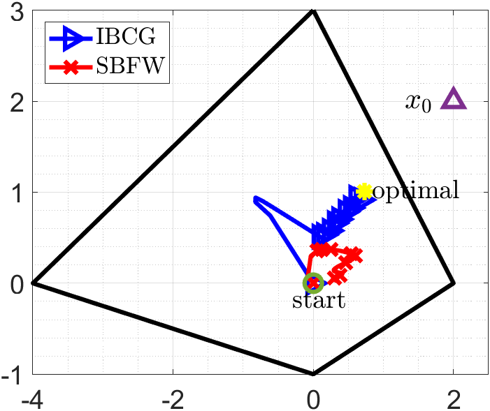
Figure 1: The performance of IBCG (blue) vs SBFW (red) on Problem 13 when $\mu_{g}=1$. Plots from left to right are trajectories of $\theta_{k}$ and $f(\lambda_{k},\theta_{k})-f^{*}$.

5.2 Matrix Completion with Denoising

In this section, we study the performance of our proposed IBCG algorithm for solving matrix completion with denoising problem in (2.1). The experimental setup we adopt is aligned with the methodology used in [MHK20]. In particular, we create an observation matrix $M=\hat{X}+E$. In this setting $\hat{X}=WW^{T}$ where $W\in\mathbb{R}^{n\times r}$ containing normally distributed independent entries, and $E=\hat{n}(L+L^{T})$ is a noise matrix where $L\in\mathbb{R}^{n\times n}$ containing normally distributed independent entries and $\hat{n}\in(0,1)$ is the noise factor. During the simulation process, we set $n=250$, $r=10$, and $\alpha=\|\hat{X}\|_{*}$. Additionally, we establish the set of observed entries $\Omega$ by randomly sampling $M$ entries with a probability of 0.8. Initially, we set $\hat{n}$ to be 0.5 and employ the IBCG algorithm to solve the problem described in (2.1). To evaluate the performance of our proposed method, we compare it with state-of-the-art methods in the literature for constrained bilevel optimization problems. In particular, We compare the performance of IBCG with other single-loop projection-based and projection-free bi-level algorithms TTSA [HWWY20] and SBFW [ABTR22], respectively. We set $\lambda_{1}=\lambda_{2}=0.05$, and set the maximum number of iteration as $10^{4}$. It should be noted that we consider pseudo-Huber loss defined by $\mathcal{R}_{\delta}(\mathbf{V})=\sum_{i,j}\delta^{2}(\sqrt{1+(\mathbf{V}_{ij}/\delta)^{2}}-1)$ as a regularization term to induce sparsity and set $\delta=0.9$. The performance is analyzed based on the normalized error, defined as $\bar{e}=\frac{\sum_{(i,j)\in\Omega}(X_{i,j}-\hat{X}_{i,j})^{2}}{\sum_{(i,j)\in\Omega}(\hat{X}_{i,j})^{2}}$, where $X$ is the matrix generated by the algorithm. Figure 2 illustrates the progression of the normalized error over time as well as $\|\nabla_{y}g(x_{k},y_{k})\|$ and the value of the upper-level objective function. We note that SBFW algorithm suffers from a slower theoretical convergence rate compared to projection-based schemes, but our proposed method outperforms other algorithms by achieving lower values of $\|\nabla_{y}g(x_{k},y_{k})\|$ and slightly better performance in terms of the normalized error values. This gain comes from the projection-free nature of the proposed algorithm and its fast convergence since we are no longer required to perform a complicated projection at each iteration.

Figure 2: The performance of IBCG (blue) vs SBFW (red) and TTSA (yellow) on Problem 2.1. Plots from left to right are trajectories of normalized error $(\bar{e})$, $\|\nabla g_{y}(x_{k},y_{k})\|$, and $f(x_{k},y_{k})$ over time.

6 Conclusion

In this paper, we focused on the constrained bilevel optimization problem that has a wide range of applications in learning problems. We proposed a novel single-loop projection-free method based on nested approximation techniques, which surpasses current approaches by achieving improved per-iteration complexity. Additionally, it offers optimal convergence rate guarantees that match the best-known complexity of projection-free algorithms for solving convex constrained single-level optimization problems. In particular, we proved that our proposed method requires approximately $\tilde{\mathcal{O}}(\epsilon^{-1})$ iterations to find an $\epsilon$-optimal solution when the upper-level objective function $f$ is convex, and approximately $\mathcal{O}(\epsilon^{-2})$ to find an $\epsilon$-stationary point when $f$ is non-convex. Our numerical results also showed superior performance of our IBCG algorithm compared to existing algorithms.

Acknowledgements

The research of N. Abolfazli and E. Yazdandoost Hamedani is supported by NSF Grant 2127696. The research of R. Jiang and A. Mokhtari is supported in part by NSF Grants 2127697, 2019844, and 2112471, ARO Grant W911NF2110226, the Machine Learning Lab (MLL) at UT Austin, and the Wireless Networking and Communications Group (WNCG) Industrial Affiliates Program.

Appendix

In section A, we establish technical lemmas based on the assumptions considered in the paper. These lemmas characterize important properties of problem 1. Notably, Lemma 2.1 is instrumental in understanding the properties associated with problem 1. Moving on to section B, we present a series of lemmas essential for deriving the rate results of the proposed algorithm. Among them, Lemma 3.1 quantifies the error between the approximated direction $F_{k}$ and $\nabla\ell(\mathbf{x}_{k})$. This quantification plays a crucial role in establishing the one-step improvement lemma (see Lemma B.4). Next, we provide the proofs of Theorem 4.1 and Corollary 4.2 in sections C and D, respectively, that support the results presented in the paper for the convex scenario. Finally, in sections E and F we provide the proofs for Theorem 4.3 along with Corollary 4.4 for the nonconvex scenario.

Appendix A Supporting Lemmas

In this section, we provide detailed explanations and proofs for the lemmas supporting the main results of the paper.

A.1 Proof of Lemma 2.1

(I) Recall that $\mathbf{y}^{*}(\mathbf{x})$ is the minimizer of the lower-level problem whose objective function is strongly convex, therefore,

$$\mu_{g}\left\|\mathbf{y}^{*}(\mathbf{x})-\mathbf{y}^{*}(\bar{\mathbf{x}})\right\|^{2} \leq\langle{\nabla_{y}g(\mathbf{x},\mathbf{y}^{*}(\mathbf{x}))-\nabla_{y}g(\mathbf{x},\mathbf{y}^{*}(\bar{\mathbf{x}})),\mathbf{y}^{*}(\mathbf{x})-\mathbf{y}^{*}(\bar{\mathbf{x}})}\rangle$$

$$=\langle{\nabla_{y}g(\bar{\mathbf{x}},\mathbf{y}^{*}(\bar{\mathbf{x}}))-\nabla_{y}g(\mathbf{x},\mathbf{y}^{*}(\bar{\mathbf{x}})),\mathbf{y}^{*}(\mathbf{x})-\mathbf{y}^{*}(\bar{\mathbf{x}})}\rangle$$

Note that $\nabla_{y}g(\mathbf{x},\mathbf{y}^{*}(\mathbf{x}))=\nabla_{y}g(\bar{\mathbf{x}},\mathbf{y}^{*}(\bar{\mathbf{x}}))=0$. Using the Cauchy-Schwartz inequality we have:

$$\mu_{g}\left\|\mathbf{y}^{*}(\mathbf{x})-\mathbf{y}^{*}(\bar{\mathbf{x}})\right\|^{2} \leq\|\nabla_{y}g(\bar{\mathbf{x}},\mathbf{y}^{*}(\bar{\mathbf{x}}))-\nabla_{y}g(\mathbf{x},\mathbf{y}^{*}(\bar{\mathbf{x}}))\|\|\mathbf{y}^{*}(\mathbf{x})-\mathbf{y}^{*}(\bar{\mathbf{x}})\|$$

$$\leq\textcolor{black}{C_{yx}^{g}}\|\mathbf{x}-\bar{\mathbf{x}}\|\|\mathbf{y}^{*}(\mathbf{x})-\mathbf{y}^{*}(\bar{\mathbf{x}})\|$$

where the blacklast inequality is obtained by using the blackAssumption 2.2. blackTherefore, we conclude that $\mu_{g}\left\|\mathbf{y}^{*}(\mathbf{x})-\mathbf{y}^{*}(\bar{\mathbf{x}})\right\|\leq C_{yx}^{g}\|\mathbf{x}-\bar{\mathbf{x}}\|$ which leads to the desired result in part (I).

(II) We first show that the function $\mathbf{x}\mapsto\nabla_{y}f(\mathbf{x},\mathbf{y}^{*}(\mathbf{x}))$ is Lipschitz continuous. To see this, note that for any $\mathbf{x},\bar{\mathbf{x}}\in\mathcal{X}$, we have

$$\|\nabla_{y}f(\mathbf{x},\mathbf{y}^{*}(\mathbf{x}))-\nabla_{y}f(\bar{\mathbf{x}},\mathbf{y}^{*}(\bar{\mathbf{x}}))\| \leq L_{yx}^{f}\|\mathbf{x}-\bar{\mathbf{x}}\|+L_{yy}^{f}\|\mathbf{y}^{*}(\mathbf{x})-\mathbf{y}^{*}(\bar{\mathbf{x}})\|$$

$$\leq\Bigl{(}L_{yx}^{f}+\frac{L_{yy}^{f}\textcolor{black}{C_{yx}^{g}}}{\mu_{g}}\Bigr{)}\|\mathbf{x}-\bar{\mathbf{x}}\|,$$

where in the last inequality we used Lemma 2.1-(I). Since $\mathcal{X}$ is bounded, we also have $\|\mathbf{x}-\bar{\mathbf{x}}\|\leq D_{\mathcal{X}}$. Therefore, letting $\bar{\mathbf{x}}=\mathbf{x}^{*}$ in the above inequality and using the triangle inequality, we have

$$\|\nabla_{y}f(\mathbf{x},\mathbf{y}^{*}(\mathbf{x}))\|\leq\Bigl{(}L_{yx}^{f}+\frac{L_{yy}^{f}\textcolor{black}{C_{yx}^{g}}}{\mu_{g}}\Bigr{)}D_{\mathcal{X}}+\|\nabla_{y}f(\textcolor{black}{\mathbf{x}^{*}},\mathbf{y}^{*}(\textcolor{black}{\mathbf{x}^{*}}))\|.$$

Thus, we complete the proof by letting $C_{y}^{f}=\Bigl{(}L_{yx}^{f}+\frac{L_{yy}^{f}\textcolor{black}{C_{yx}^{g}}}{\mu_{g}}\Bigr{)}D_{\mathcal{X}}+\|\nabla_{y}f(\textcolor{black}{\mathbf{x}^{*}},\mathbf{y}^{*}(\textcolor{black}{\mathbf{x}^{*}}))\|$.

Before proceeding to show the result of part (III) of Lemma 2.1, we first establish an auxiliary lemma stated next.

Lemma A.1.

Under the premises of Lemma 2.1, we have that for any $\mathbf{x},\bar{\mathbf{x}}\in\mathcal{X}$, $\left\|\mathbf{v}(\mathbf{x})-\mathbf{v}(\bar{\mathbf{x}})\right\|\leq\mathbf{C}_{\mathbf{v}}\left\|\mathbf{x}-\bar{\mathbf{x}}\right\|$ for some $\mathbf{C}_{\mathbf{v}}\geq 0$.

Proof.

We start the proof by recalling that $\mathbf{v}(\mathbf{x})=\nabla_{yy}g(\mathbf{x},\mathbf{y}^{*}(\mathbf{x}))^{-1}\nabla_{y}f(\mathbf{x},\mathbf{y}^{*}(\mathbf{x}))$. Next, adding and subtracting $\nabla_{yy}g(\mathbf{x},\mathbf{y}^{*}(\mathbf{x}))\nabla_{y}f(\bar{\mathbf{x}},\mathbf{y}^{*}(\bar{\mathbf{x}}))$ followed by a triangle inequality leads to,

$$\|\mathbf{v}(\mathbf{x})-\mathbf{v}(\bar{\mathbf{x}})\|$$

$$=\|[\nabla_{yy}g(\mathbf{x},\mathbf{y}^{*}(\mathbf{x}))]^{-1}\nabla_{y}f(\mathbf{x},\mathbf{y}^{*}(\mathbf{x}))-[\nabla_{yy}g(\bar{\mathbf{x}},\mathbf{y}^{*}(\bar{\mathbf{x}}))]^{-1}\nabla_{y}f(\bar{\mathbf{x}},\mathbf{y}^{*}(\bar{\mathbf{x}}))\|$$

$$\leq\|[\nabla_{yy}g(\mathbf{x},\mathbf{y}^{*}(\mathbf{x}))]^{-1}\big{(}\nabla_{y}f(\mathbf{x},\mathbf{y}^{*}(\mathbf{x}))-\nabla_{y}f(\bar{\mathbf{x}},\mathbf{y}^{*}(\bar{\mathbf{x}}))\big{)}\|+\|\big{(}[\nabla_{yy}g(\mathbf{x},\mathbf{y}^{*}(\mathbf{x}))]^{-1}$$

$$-[\nabla_{yy}g(\bar{\mathbf{x}},\mathbf{y}^{*}(\bar{\mathbf{x}}))]^{-1}\big{)}\nabla_{y}f(\bar{\mathbf{x}},\mathbf{y}^{*}(\bar{\mathbf{x}}))\|$$

$$\leq\frac{1}{\mu_{g}}\big{(}{L_{yx}^{f}}\|\mathbf{x}-\bar{\mathbf{x}}\|+{L_{yy}^{f}}\|\mathbf{y}^{*}(\mathbf{x})-\mathbf{y}^{*}(\bar{\mathbf{x}})\|\big{)}+C_{y}^{f}\|[\nabla_{yy}g(\mathbf{x},\mathbf{y}^{*}(\mathbf{x}))]^{-1}-[\nabla_{yy}g(\bar{\mathbf{x}},\mathbf{y}^{*}(\bar{\mathbf{x}}))]^{-1}\|,$$ (14)

where in the last inequality we used Assumptions 2.1 and 2.2-(iii) blackalong with the premises of Lemma 2.1-(II). Moreover, for any invertible matrices $H_{1}$ and $H_{2}$, we have that

$$\|H_{2}^{-1}-H_{1}^{-1}\|=\|H_{1}^{-1}\big{(}H_{1}-H_{2}\big{)}H_{2}^{-1}\|\leq\|H_{1}^{-1}\|\|H_{2}^{-1}\|\|H_{1}-H_{2}\|.$$ (15)

Therefore, using the result of Lemma 2.1-(I) and (15) we can further bound inequality (A.1) as follows,

$$\left\|\mathbf{v}(\mathbf{x})-\mathbf{v}(\bar{\mathbf{x}})\right\|$$

$$\leq\frac{1}{\mu_{g}}\big{(}{L_{yx}^{f}}\|\mathbf{x}-\bar{\mathbf{x}}\|+{L_{yy}^{f}}\mathbf{L}_{\mathbf{y}}\|\mathbf{x}-\bar{\mathbf{x}}\|\big{)}+C_{y}^{f}\|[\nabla_{yy}g(\mathbf{x},\mathbf{y}^{*}(\mathbf{x}))]^{-1}-[\nabla_{yy}g(\bar{\mathbf{x}},\mathbf{y}^{*}(\bar{\mathbf{x}}))]^{-1}\|$$

$$\leq\frac{1}{\mu_{g}}\big{(}{L_{yx}^{f}}+{L_{yy}^{f}}\mathbf{L}_{\mathbf{y}}\big{)}\|\mathbf{x}-\bar{\mathbf{x}}\|+{\frac{C_{y}^{f}}{\mu_{g}^{2}}L_{yy}^{g}\bigl{(}\|\mathbf{x}-\bar{\mathbf{x}}\|+\|\mathbf{y}^{*}(\mathbf{x})-\mathbf{y}^{*}(\bar{\mathbf{x}})\|\bigr{)}}$$

$$=\bigl{(}{\frac{L_{yx}^{f}+L_{yy}^{f}\mathbf{L}_{\mathbf{y}}}{\mu_{g}}+\frac{C_{y}^{f}L_{yy}^{g}}{\mu_{g}^{2}}(1+\mathbf{L}_{\mathbf{y}})}\bigr{)}\|\mathbf{x}-\bar{\mathbf{x}}\|.$$

The result follows by letting $\mathbf{C}_{\mathbf{v}}=\frac{L_{yx}^{f}+L_{yy}^{f}\mathbf{L}_{\mathbf{y}}}{\mu_{g}}+\frac{C_{y}^{f}L_{yy}^{g}}{\mu_{g}^{2}}(1+\mathbf{L}_{\mathbf{y}})$. ∎

(III) We start proving part (III) using the definition of $\nabla\ell(\mathbf{x})$ stated in (7a). Using the triangle inequality we obtain,

$$\|\nabla\ell(\mathbf{x})-\nabla\ell(\bar{\mathbf{x}})\|$$

$$\quad=\|\nabla_{x}f(\mathbf{x},\mathbf{y}^{*}(\mathbf{x}))-\nabla_{yx}g({\mathbf{x}},\mathbf{y}^{*}({\mathbf{x}}))\mathbf{v}({\mathbf{x}})-\big{(}\nabla_{x}f(\bar{\mathbf{x}},\mathbf{y}^{*}(\bar{\mathbf{x}}))-\nabla_{yx}g(\bar{\mathbf{x}},\mathbf{y}^{*}(\bar{\mathbf{x}}))\mathbf{v}(\bar{\mathbf{x}})\big{)}\|$$

$$\quad\leq\|\nabla_{x}f(\mathbf{x},\mathbf{y}^{*}(\mathbf{x}))-\nabla_{x}f(\bar{\mathbf{x}},\mathbf{y}^{*}(\bar{\mathbf{x}}))\|+\|\big{[}\nabla_{yx}g(\bar{\mathbf{x}},\mathbf{y}^{*}(\bar{\mathbf{x}}))\mathbf{v}(\bar{\mathbf{x}})-\nabla_{yx}g(\bar{\mathbf{x}},\mathbf{y}^{*}(\bar{\mathbf{x}}))\mathbf{v}(\mathbf{x})\big{]}$$

$$\qquad+\big{[}\nabla_{yx}g(\bar{\mathbf{x}},\mathbf{y}^{*}(\bar{\mathbf{x}}))\mathbf{v}(\mathbf{x})-\nabla_{yx}g({\mathbf{x}},\mathbf{y}^{*}({\mathbf{x}}))\mathbf{v}({\mathbf{x}})\big{]}\|$$ (16)

blackwhere the second term of the RHS follows from adding and subtracting the term $\nabla_{yx}g(\bar{\mathbf{x}},\mathbf{y}^{*}(\bar{\mathbf{x}}))\mathbf{v}(\mathbf{x})$. Next, from Assumptions 2.1-(i) and 2.2-(v) together with the triangle inequality we conclude that

$$\|\nabla\ell(\mathbf{x})-\nabla\ell(\bar{\mathbf{x}})\| \leq L_{xx}^{f}\|\mathbf{x}-\bar{\mathbf{x}}\|+L_{xy}^{f}\|\mathbf{y}^{*}(\mathbf{x})-\mathbf{y}^{*}(\bar{\mathbf{x}})\|\ +C_{yx}^{g}\|\mathbf{v}(\bar{\mathbf{x}})-\mathbf{v}(\mathbf{x})\|$$

$$\quad+\frac{C_{y}^{f}}{\mu_{g}}\|\nabla_{yx}g(\bar{\mathbf{x}},\mathbf{y}^{*}(\bar{\mathbf{x}}))-\nabla_{yx}g({\mathbf{x}},\mathbf{y}^{*}({\mathbf{x}}))\|$$ (17)

Note that in the last inequality, we use the fact that $\|\mathbf{v}(\mathbf{x})\|=\|[\nabla_{yy}g(\mathbf{x},\mathbf{y}^{*}(\mathbf{x}))]^{-1}\nabla_{y}f(\mathbf{x},\mathbf{y}^{*}(\mathbf{x}))\|\leq\frac{C_{y}^{f}}{\mu_{g}}$. Combining the result of Lemma 2.1 part (I) and (II) with the Assumption 2.2-(iv) leads to

$$\|\nabla\ell(\mathbf{x})-\nabla\ell(\bar{\mathbf{x}})\| \leq L_{xx}^{f}\|\mathbf{x}-\bar{\mathbf{x}}\|+L_{xy}^{f}\mathbf{L}_{\mathbf{y}}\|\mathbf{x}-\bar{\mathbf{x}}\|+C_{yx}^{g}\mathbf{C}_{\mathbf{v}}\|\mathbf{x}-\bar{\mathbf{x}}\|$$

$$\quad+\frac{C_{y}^{f}}{\mu_{g}}L_{yx}^{g}\bigl{(}\|\mathbf{x}-\bar{\mathbf{x}}\|+\|\mathbf{y}^{*}(\mathbf{x})-\mathbf{y}^{*}(\bar{\mathbf{x}})\|\bigr{)}$$

$$\leq L_{xx}^{f}\|\mathbf{x}-\bar{\mathbf{x}}\|+L_{xy}^{f}\mathbf{L}_{\mathbf{y}}\|\mathbf{x}-\bar{\mathbf{x}}\|+C_{yx}^{g}\mathbf{C}_{\mathbf{v}}\|\mathbf{x}-\bar{\mathbf{x}}\|$$

$$\quad+\frac{C_{y}^{f}}{\mu_{g}}L_{yx}^{g}\bigl{(}\|\mathbf{x}-\bar{\mathbf{x}}\|+\mathbf{L}_{\mathbf{y}}\|\mathbf{x}-\bar{\mathbf{x}}\|\bigr{)}$$

$$\leq\big{(}L_{xx}^{f}+{L_{xy}^{f}}\mathbf{L}_{\mathbf{y}}+C_{yx}^{g}\mathbf{C}_{\mathbf{v}}+\frac{C_{y}^{f}}{\mu_{g}}L_{yx}^{g}(1+\mathbf{L}_{\mathbf{y}})\big{)}\|\mathbf{x}-\bar{\mathbf{x}}\|$$ (18)

The desired result can be obtained by letting $\mathbf{L}_{\ell}=L_{xx}^{f}+{L_{xy}^{f}}\mathbf{L}_{\mathbf{y}}+C_{yx}^{g}\mathbf{C}_{\mathbf{v}}+\frac{C_{y}^{f}}{\mu_{g}}L_{yx}^{g}(1+\mathbf{L}_{\mathbf{y}})$. ∎

Appendix B Required Lemmas for Theorem 4.1 and 4.3

blackBefore we proceed to the proofs of Theorems 4.1 and 4.3, we present the following technical lemmas which quantify the error between the approximated solution $\mathbf{y}_{k}$ and $\mathbf{y}^{*}(\mathbf{x}_{k})$, as well as between $\mathbf{w}_{k+1}$ and $\mathbf{v}(\mathbf{x}_{k})$.

Lemma B.1.

blackSuppose Assumption 2.2 holds. Let $\{(\mathbf{x}_{k},\mathbf{y}_{k})\}_{k\geq 0}$ be the sequence generated by Algorithm 1, such that $\alpha=2/(\mu_{g}+L_{g})$. Then, for any $k\geq 0$

$$\|\mathbf{y}_{k}-\mathbf{y}^{*}(\mathbf{x}_{k})\|\leq\beta^{k}\|\mathbf{y}_{0}-\mathbf{y}^{*}(\mathbf{x}_{0})\|+\mathbf{L}_{\mathbf{y}}D_{\mathcal{X}}\sum_{i=0}^{k-1}\gamma_{i}\beta^{k-i},$$ (19)

where $\beta\triangleq(L_{g}-\mu_{g})/(L_{g}+\mu_{g})$.

Proof.

blackWe begin the proof by characterizing the one-step progress of the lower-level iterate sequence $\{\mathbf{y}_{k}\}_{k}$. Indeed, at iteration $k$ we aim to approximate $\mathbf{y}^{*}(\mathbf{x}_{k+1})=\operatorname*{\arg\!\min}_{\mathbf{y}}g(\mathbf{x}_{k+1},\mathbf{y})$. According to the update of $\mathbf{y}_{k+1}$ we observe that

$$\|\mathbf{y}_{k+1}-\mathbf{y}^{*}(\mathbf{x}_{k+1})\|^{2} =\|\mathbf{y}_{k}-\mathbf{y}^{*}(\mathbf{x}_{k+1})-\alpha\nabla_{y}g(\mathbf{x}_{k+1},\mathbf{y}_{k})\|^{2}$$

$$=\|\mathbf{y}_{k}-\mathbf{y}^{*}(\mathbf{x}_{k+1})\|^{2}-2\alpha\langle\nabla_{y}g(\mathbf{x}_{k+1},\mathbf{y}_{k}),\mathbf{y}_{k}-\mathbf{y}^{*}(\mathbf{x}_{k+1})\rangle$$

$$\quad+\alpha^{2}\|\nabla_{y}g(\mathbf{x}_{k+1},\mathbf{y}_{k})\|^{2}.$$ (20)

Moreover, from Assumption 2.2 we have that

$$\langle\nabla_{y}g(\mathbf{x}_{k+1},\mathbf{y}_{k}),\mathbf{y}_{k}-\mathbf{y}^{*}(\mathbf{x}_{k+1})\rangle\geq\frac{\mu_{g}L_{g}}{\mu_{g}+L_{g}}\|\mathbf{y}_{k}-\mathbf{y}^{*}(\mathbf{x}_{k+1})\|^{2}+\frac{1}{\mu_{g}+L_{g}}\|\nabla_{y}g(\mathbf{x}_{k+1},\mathbf{y}_{k})\|^{2}.$$ (21)

The inequality in (B) together with (21) imply that

$$\|\mathbf{y}_{k+1}-\mathbf{y}^{*}(\mathbf{x}_{k+1})\|^{2} \leq\|\mathbf{y}_{k}-\mathbf{y}^{*}(\mathbf{x}_{k+1})\|^{2}-\frac{2\alpha\mu_{g}L_{g}}{\mu_{g}+L_{g}}\|\mathbf{y}_{k}-\mathbf{y}^{*}(\mathbf{x}_{k+1})\|^{2}$$

$$\quad+\Big{(}\alpha^{2}-\frac{2\alpha}{\mu_{g}+L_{g}}\Big{)}\|\nabla_{y}g(\mathbf{x}_{k+1},\mathbf{y}_{k})\|^{2}.$$ (22)

Setting the step-size $\alpha=\frac{2}{\mu_{g}+L_{g}}$ in (B) leads to

$$\|\mathbf{y}_{k+1}-\mathbf{y}^{*}(\mathbf{x}_{k+1})\|^{2} \leq\Big{(}\frac{\mu_{g}-L_{g}}{\mu_{g}+L_{g}}\Big{)}^{2}\|\mathbf{y}_{k}-\mathbf{y}^{*}(\mathbf{x}_{k+1})\|^{2}$$ (23)

blackNext, recall that $\beta=(L_{g}-\mu_{g})/(L_{g}+\mu_{g})$. Using the triangle inequality and Part (I) of Lemma 2.1 we conclude that

$$\|\mathbf{y}_{k+1}-\mathbf{y}^{*}(\mathbf{x}_{k+1})\| \leq\beta\|\mathbf{y}_{k}-\mathbf{y}^{*}(\mathbf{x}_{k+1})\|$$

$$\leq\beta\Big{[}\|\mathbf{y}_{k}-\mathbf{y}^{*}(\mathbf{x}_{k})\|+\|\mathbf{y}^{*}({\mathbf{x}_{k}})-\mathbf{y}^{*}(\mathbf{x}_{k+1})\|\Big{]}$$

$$\leq\beta\Big{[}\|\mathbf{y}_{k}-\mathbf{y}^{*}(\mathbf{x}_{k})\|+\mathbf{L}_{\mathbf{y}}\|\mathbf{x}_{k}-\mathbf{x}_{k+1}\|\Big{]}.$$ (24)

blackMoreover, from the update of $\mathbf{x}_{k+1}$ in Algorithm 1 and boundedness of $\mathcal{X}$ we have that $\left\|\mathbf{x}_{k+1}-\mathbf{x}_{k}\right\|\leq\gamma_{k}\textcolor{black}{D_{\mathcal{X}}}$. blackTherefore, using this inequality within (B) leads to

$$\left\|\mathbf{y}_{k+1}-\mathbf{y}^{*}(\mathbf{x}_{k+1})\right\|\leq\beta\left\|\mathbf{y}_{k}-\mathbf{y}^{*}(\mathbf{x}_{k})\right\|+\beta\gamma_{k}\mathbf{L}_{\mathbf{y}}D_{\mathcal{X}}.$$

Finally, the desired result can be deduced from the above inequality recursively. ∎

Previously, in Lemma B.1 blackwe quantified how close the approximation $\mathbf{y}_{k}$ is from the optimal solution $\mathbf{y}^{*}(\mathbf{x}_{k})$ of the inner problem. Now, in the following Lemma, we will find an upper bound for the error of approximating $\mathbf{v}(\mathbf{x}_{k})$ via $\mathbf{w}_{k+1}$.

Lemma B.2.

Let $\{(\mathbf{x}_{k},\mathbf{w}_{k})\}_{k\geq 0}$ be the sequence generated by Algorithm 1, such that $\gamma_{k}=\gamma$. Define $\rho_{k}\triangleq(1-\eta_{k}\mu_{g})$ and $\mathbf{C}_{1}\triangleq L_{yy}^{g}\frac{C_{y}^{f}}{\mu_{g}}+L_{yy}^{f}$. blackUnder Assumptions 2.1 and 2.2 we have that for any $k\geq 0$,

$$\|{\mathbf{w}_{k+1}}-\mathbf{v}(\mathbf{x}_{k})\|\leq\rho_{k}\|{\mathbf{w}_{k}}-\mathbf{v}(\mathbf{x}_{k-1})\|+\rho_{k}\mathbf{C}_{\mathbf{v}}\gamma D_{\mathcal{X}}+\eta_{k}\mathbf{C}_{1}\big{(}\beta^{k}D_{0}^{y}+\mathbf{L}_{\mathbf{y}}\gamma\frac{\beta}{1-\beta}D_{\mathcal{X}}\big{)}.$$ (25)

Proof.

One can easily verify that $\mathbf{v}(\mathbf{x}_{k})=\mathbf{v}(\mathbf{x}_{k})-\eta_{k}\bigl{(}\nabla_{yy}g(\mathbf{x}_{k},\mathbf{y}^{*}(\mathbf{x}_{k}))\mathbf{v}(\mathbf{x}_{k})-\nabla_{y}f(\mathbf{x}_{k},\mathbf{y}^{*}(\mathbf{x}_{k}))\bigr{)}$ from the optimality condition of (8). blackNow using definition of $\mathbf{w}_{k+1}$ we can write

$$\|{\mathbf{w}_{k+1}}-\mathbf{v}(\mathbf{x}_{k})\| =\Big{\|}\Big{(}\mathbf{w}_{k}-\eta_{k}(\nabla_{yy}g(\mathbf{x}_{k},\mathbf{y}_{k})\mathbf{w}_{k}-\nabla_{y}f(\mathbf{x}_{k},\mathbf{y}_{k}))\Big{)}-\Big{(}\mathbf{v}(\mathbf{x}_{k})$$

$$\quad-\eta_{k}\big{(}\nabla_{yy}g(\mathbf{x}_{k},\mathbf{y}^{*}(\mathbf{x}_{k}))\mathbf{v}(\mathbf{x}_{k})-\nabla_{y}f(\mathbf{x}_{k},\mathbf{y}^{*}(\mathbf{x}_{k}))\big{)}\Big{)}\Big{\|}$$

$$=\Big{\|}\Big{(}I-\eta_{k}\nabla_{yy}g(\mathbf{x}_{k},\mathbf{y}_{k})\Big{)}(\mathbf{w}_{k}-\mathbf{v}(\mathbf{x}_{k}))-\eta_{k}\Big{(}\nabla_{yy}g(\mathbf{x}_{k},\mathbf{y}_{k})$$

$$\quad-\nabla_{yy}g(\mathbf{x}_{k},\mathbf{y}^{*}(\mathbf{x}_{k}))\Big{)}\mathbf{v}(\mathbf{x}_{k})+\eta_{k}\Big{(}\nabla_{y}f(\mathbf{x}_{k},\mathbf{y}^{*}(\mathbf{x}_{k}))-\nabla_{y}f(\mathbf{x}_{k},\mathbf{y}_{k})\Big{)}\Big{\|},$$ (26)

where the last equality is obtained by adding and subtracting the term $(I-\eta_{k}\nabla_{yy}g(\mathbf{x}_{k},\mathbf{y}_{k}))\mathbf{v}(\mathbf{x}_{k})$. Next, using Assumptions 2.1 and 2.2 along with the application of the triangle inequality we obtain

$$\|{\mathbf{w}_{k+1}}-\mathbf{v}(\mathbf{x}_{k})\| \leq(1-\eta_{k}\mu_{g})\|{\mathbf{w}_{k}}-\mathbf{v}(\mathbf{x}_{k})\|+\eta_{k}L_{yy}^{g}\|\mathbf{y}_{k}-\mathbf{y}^{*}(\mathbf{x}_{k})\|\|\mathbf{v}(\mathbf{x}_{k})\|$$

$$\quad+\eta_{k}L_{yy}^{f}\|\mathbf{y}_{k}-\mathbf{y}^{*}(\mathbf{x}_{k})\|.$$ (27)

Note that $\|\mathbf{v}(\mathbf{x}_{k})\|=\|[\nabla_{yy}g(\mathbf{x},\mathbf{y}^{*}(\mathbf{x}))]^{-1}\nabla_{y}f(\mathbf{x},\mathbf{y}^{*}(\mathbf{x}))\|\leq\frac{C_{y}^{f}}{\mu_{g}}$. Now, by adding and subtracting $\mathbf{v}(\mathbf{x}_{k-1})$ to the term $\|{\mathbf{w}_{k}}-\mathbf{v}(\mathbf{x}_{k})\|$ followed by triangle inequality application we can conclude that

$$\|{\mathbf{w}_{k+1}}-\mathbf{v}(\mathbf{x}_{k})\| \leq(1-\eta_{k}\mu_{g})\|{\mathbf{w}_{k}}-\mathbf{v}(\mathbf{x}_{k-1})\|+(1-\eta_{k}\mu_{g})\|\mathbf{v}(\mathbf{x}_{k-1})-\mathbf{v}(\mathbf{x}_{k})\|$$

$$\quad+\eta_{k}\Big{(}L_{yy}^{g}\frac{C_{y}^{f}}{\mu_{g}}+L_{yy}^{f}\Big{)}\|\mathbf{y}_{k}-\mathbf{y}^{*}(\mathbf{x}_{k})\|.$$ (28)

Therefore, using the result of Lemma B.1, we can further bound inequality (28) as follows

$$\|{\mathbf{w}_{k+1}}-\mathbf{v}(\mathbf{x}_{k})\| \leq(1-\eta_{k}\mu_{g})\|{\mathbf{w}_{k}}-\mathbf{v}(\mathbf{x}_{k-1})\|+(1-\eta_{k}\mu_{g})\mathbf{C}_{\mathbf{v}}\|\mathbf{x}_{k-1}-\mathbf{x}_{k}\|$$

$$\quad+\eta_{k}\mathbf{C}_{1}\|\mathbf{y}_{k}-\mathbf{y}^{*}(\mathbf{x}_{k})\|$$

$$\leq\rho_{k}\|{\mathbf{w}_{k}}-\mathbf{v}(\mathbf{x}_{k-1})\|+\rho_{k}\mathbf{C}_{\mathbf{v}}\gamma D_{\mathcal{X}}+\eta_{k}\mathbf{C}_{1}\big{(}\beta^{k}D_{0}^{y}+\mathbf{L}_{\mathbf{y}}\gamma\frac{\beta}{1-\beta}D_{\mathcal{X}}\big{)}$$ (29)

where the last inequality follows from the boundedness assumption of set $\mathcal{X}$, recalling that $D_{0}^{y}=\|\mathbf{y}_{0}-\mathbf{y}^{*}(\mathbf{x}_{0})\|$, and the fact that $\sum_{i=0}^{k-1}\beta^{k-i}\leq\frac{\beta}{1-\beta}$. ∎

Lemma B.3.

Let $\{(\mathbf{x}_{k},\mathbf{w}_{k})\}_{k\geq 0}$ be the sequence generated by Algorithm 1 with step-size $\eta_{k}=\eta<\frac{1-\beta}{\mu_{g}}$ where $\beta$ is defined in Lemma B.1. Suppose that Assumption 2.2 holds and $\mathbf{v}(\mathbf{x}_{-1})=\mathbf{v}(\mathbf{x}_{0})$, then for any $K\geq 1$,

$$\|\mathbf{w}_{K}-\mathbf{v}(\mathbf{x}_{K-1})\|\leq\rho^{K}\|{\mathbf{w}_{0}}-\mathbf{v}(\mathbf{x}_{0})\|+\frac{\gamma\rho\mathbf{C}_{\mathbf{v}}D_{\mathcal{X}}}{1-\rho}+\frac{\eta\mathbf{C}_{1}D_{0}^{y}\rho^{K+1}}{\rho-\beta}+\frac{\gamma\eta\beta\mathbf{C}_{1}\mathbf{L}_{\mathbf{y}}D_{\mathcal{X}}}{(1-\rho)(1-\beta)},$$ (30)

where $\rho\triangleq 1-\eta\mu_{g}$.

Proof.

Applying the result of Lemma B.2 recursively for $k=0$ to $K-1$, one can conclude that

$$\|\mathbf{w}_{K}-\mathbf{v}(\mathbf{x}_{K-1})\| \leq\rho^{K}\|{\mathbf{w}_{0}}-\mathbf{v}(\mathbf{x}_{0})\|+\mathbf{C}_{\mathbf{v}}\gamma D_{\mathcal{X}}\sum_{i=1}^{K}\rho^{i}+\eta\mathbf{C}_{1}\sum_{i=0}^{K}\big{(}\beta^{i}D_{0}^{y}+\gamma\mathbf{L}_{\mathbf{y}}D_{\mathcal{X}}\frac{\beta}{1-\beta}\big{)}\rho^{K-i}$$

$$\leq\rho^{K}\|{\mathbf{w}_{0}}-\mathbf{v}(\mathbf{x}_{0})\|+\frac{\rho}{1-\rho}\mathbf{C}_{\mathbf{v}}\gamma D_{\mathcal{X}}+\eta\mathbf{C}_{1}D_{0}^{y}\big{(}\sum_{i=0}^{K}\beta^{i}\rho^{K-i}\big{)}$$

$$\quad+\frac{\gamma\eta\beta\mathbf{C}_{1}\mathbf{L}_{\mathbf{y}}D_{\mathcal{X}}}{1-\beta}\sum_{i=0}^{K}\rho^{K-i},$$ (31)

where the last inequality is obtained by noting that $\sum_{i=1}^{K}\rho^{i}\leq\frac{\rho}{1-\rho}$. Finally, the choice $\eta<\frac{1-\beta}{\mu_{g}}$ implies that $\beta<\rho$, hence, $\sum_{i=0}^{K}(\frac{\beta}{\rho})^{i}\leq\frac{\rho}{\rho-\beta}$ which leads to the desired result. ∎

B.1 Proof of Lemma 3.1

We begin the proof by considering the definition of $\nabla\ell(\mathbf{x}_{k})$ and $F_{k}$ followed by a triangle inequality to obtain

$$\|\nabla\ell(\mathbf{x}_{k})-F_{k}\| \leq\|\nabla_{x}f(\mathbf{x}_{k},\mathbf{y}^{*}(\mathbf{x}_{k}))-\nabla_{x}f(\mathbf{x}_{k},\mathbf{y}_{k})\|$$

$$\quad+\|\nabla_{yx}g(\mathbf{x}_{k},\mathbf{y}_{k})\mathbf{w}_{k+1}-\nabla_{yx}g(\mathbf{x}_{k},\mathbf{y}^{*}(\mathbf{x}_{k}))\mathbf{v}(\mathbf{x}_{k})\|$$ (32)

Combining Assumption 2.1-(i) together with adding and subtracting $\nabla_{yx}g(\mathbf{x}_{k},\mathbf{y}_{k})\mathbf{v}(\mathbf{x}_{k})$ to the second term of RHS lead to

$$\|\nabla\ell(\mathbf{x}_{k})-F_{k}\| \leq\textcolor{black}{L_{xy}^{f}}\|\mathbf{y}_{k}-\mathbf{y}^{*}(\mathbf{x}_{k})\|+\|\nabla_{yx}g(\mathbf{x}_{k},\mathbf{y}_{k})\big{(}\mathbf{w}_{k+1}-\mathbf{v}(\mathbf{x}_{k})\big{)}+\big{(}\nabla_{yx}g(\mathbf{x}_{k},\mathbf{y}_{k})$$

$$\quad-\nabla_{yx}g(\mathbf{x}_{k},\mathbf{y}^{*}(\mathbf{x}_{k}))\big{)}\mathbf{v}(\mathbf{x}_{k})\|$$

$$\leq\textcolor{black}{L_{xy}^{f}}\|\mathbf{y}_{k}-\mathbf{y}^{*}(\mathbf{x}_{k})\|+C_{yx}^{g}\|\mathbf{w}_{k+1}-\mathbf{v}(\mathbf{x}_{k})\|+L_{yx}^{g}\frac{C_{y}^{f}}{\mu_{g}}\|\mathbf{y}_{k}-\mathbf{y}^{*}(\mathbf{x}_{k})\|$$ (33)

where the last inequality is obtained using Assumption 2.2 and the triangle inequality. Next, utilizing Lemma B.1 and B.3 we can further provide upper-bounds for the term in RHS of (B.1) as follows

$$\|\nabla\ell(\mathbf{x}_{k})-F_{k}\| \leq\mathbf{C}_{2}\big{(}\beta^{k}D_{0}^{y}+\frac{\gamma\beta\mathbf{L}_{\mathbf{y}}D_{\mathcal{X}}}{1-\beta}\big{)}+C_{yx}^{g}\Big{(}\rho^{k+1}\|{\mathbf{w}_{0}}-\mathbf{v}(\mathbf{x}_{0})\|+\frac{\gamma\rho\mathbf{C}_{\mathbf{v}}D_{\mathcal{X}}}{1-\rho}$$

$$\quad+\frac{\eta\mathbf{C}_{1}D_{0}^{y}\rho^{k+2}}{\rho-\beta}+\frac{\gamma\eta\beta\mathbf{C}_{1}\mathbf{L}_{\mathbf{y}}D_{\mathcal{X}}}{(1-\rho)(1-\beta)}\Big{)}.$$

∎

B.2 Improvement in one step

In the following, we characterize the improvement of the objective function $\ell(\mathbf{x})$ after taking one step of Algorithm 1.

Lemma B.4.

Let $\{\mathbf{x}_{k}\}_{k=0}^{K}$ be the sequence generated by Algorithm 1. Suppose Assumption 2.1 and 2.2 hold and $\gamma_{k}=\gamma$, then for any $k\geq 0$ we have

$$\ell(\mathbf{x}_{k+1}) \leq\ell(\mathbf{x}_{k})-\gamma\mathcal{G}(\mathbf{x}_{k})+\gamma\mathbf{C}_{2}\beta^{k}D_{0}^{y}D_{\mathcal{X}}+\frac{\gamma^{2}D_{\mathcal{X}}^{2}\mathbf{L}_{\mathbf{y}}\beta}{1-\beta}+C_{yx}^{g}\Big{[}\gamma D_{\mathcal{X}}\rho^{k+1}\|{\mathbf{w}_{0}}-\mathbf{v}(\mathbf{x}_{0})\|$$

$$\quad+\frac{\gamma^{2}D_{\mathcal{X}}^{2}\rho\mathbf{C}_{\mathbf{v}}}{1-\rho}+\frac{\gamma D_{\mathcal{X}}D_{0}^{y}\mathbf{C}_{1}\eta\rho^{k+2}}{\rho-\beta}+\frac{\gamma^{2}D_{\mathcal{X}}^{2}\mathbf{L}_{\mathbf{y}}\mathbf{C}_{1}\beta\eta}{(1-\beta)(1-\rho)}\Big{]}+\frac{1}{2}\mathbf{L}_{\ell}\gamma^{2}D_{\mathcal{X}}^{2}$$ (34)

Proof.

Note that according to Lemma 2.1-(III), $\ell(\cdot)$ has a Lipschitz continuous gradient which implies that

$$\ell(\mathbf{x}_{k+1}) \leq\ell(\mathbf{x}_{k})+\gamma\langle{\nabla\ell(\mathbf{x}_{k}),\mathbf{s}_{k}-\mathbf{x}_{k}}\rangle+\frac{1}{2}\mathbf{L}_{\ell}\gamma^{2}\|\mathbf{s}_{k}-\mathbf{x}_{k}\|^{2}$$

$$=\ell(\mathbf{x}_{k})+\gamma\langle{F_{k},\mathbf{s}_{k}-\mathbf{x}_{k}}\rangle+\gamma\langle{\nabla\ell(\mathbf{x}_{k})-F_{k},\mathbf{s}_{k}-\mathbf{x}_{k}}\rangle+\frac{1}{2}\mathbf{L}_{\ell}\gamma^{2}\|\mathbf{s}_{k}-\mathbf{x}_{k}\|^{2}$$ (35)

where the last inequality follows from adding and subtracting the term $\gamma\langle{F_{k},\mathbf{s}_{k}-\mathbf{x}_{k}}\rangle$ to the RHS. Using the definition of $\mathbf{s}_{k}$ and $\mathcal{G}(x)$ we can immediately observe that

$$\langle{F_{k},\mathbf{s}_{k}-\mathbf{x}_{k}}\rangle =\min_{\mathbf{s}\in\mathcal{X}}~{}\langle{F_{k},\mathbf{s}-\mathbf{x}_{k}}\rangle$$

$$\leq\langle{F_{k},\mathbf{s}-\mathbf{x}_{k}}\rangle$$

$$=\langle{\nabla\ell(\mathbf{x}_{k}),\mathbf{s}-\mathbf{x}_{k}}\rangle+\langle{F_{k}-\nabla\ell(\mathbf{x}_{k}),\mathbf{s}-\mathbf{x}_{k}}\rangle$$

$$\leq-\mathcal{G}(\mathbf{x}_{k})+\langle{F_{k}-\nabla\ell(\mathbf{x}_{k}),\mathbf{s}-\mathbf{x}_{k}}\rangle.$$ (36)

Next, combining (35) with (36) followed by the Cauchy-Schwartz inequality leads to

$$\ell(\mathbf{x}_{k+1}) \leq\ell(\mathbf{x}_{k})-\gamma\mathcal{G}(\mathbf{x}_{k})+\gamma\|{\nabla\ell(\mathbf{x}_{k})-F_{k}\|\|\mathbf{s}_{k}-\mathbf{s}}\|+\frac{1}{2}\mathbf{L}_{\ell}\gamma^{2}\|\mathbf{s}_{k}-\mathbf{x}_{k}\|^{2}.$$ (37)

Finally, using the result of the Lemma 3.1 together with the boundedness assumption of set $\mathcal{X}$ we conclude the desired result. ∎

Appendix C Proof of Theorem 4.1

Since $\ell$ is convex, from the definition of $\mathcal{G}(\mathbf{x}_{k})$ in (4) we have:

$$\mathcal{G}(\mathbf{x}_{k})=\max_{\mathbf{s}\in\mathcal{X}}\{\langle{\nabla\ell(\mathbf{x}_{k}),\mathbf{x}_{k}-\mathbf{s}}\}\rangle\geq\langle{\nabla\ell(\mathbf{x}_{k}),\mathbf{x}_{k}-\mathbf{x}^{*}}\rangle\geq\ell(\mathbf{x}_{k})-\ell(\mathbf{x}^{*}).$$ (38)

We assume a fixed step-size in Theorem 4.1 and we set $\gamma_{k}=\gamma$. Combining the result of Lemma B.4 with (38) leads to

$$\ell(\mathbf{x}_{k+1}) \leq\ell(\mathbf{x}_{k})-\gamma(\ell(\mathbf{x}^{*})-\ell(\mathbf{x}_{k}))+\gamma\mathbf{C}_{2}\beta^{k}D_{0}^{y}D_{\mathcal{X}}+\frac{\gamma^{2}D_{\mathcal{X}}^{2}\mathbf{L}_{\mathbf{y}}\beta}{1-\beta}+C_{yx}^{g}\Big{[}\gamma D_{\mathcal{X}}\rho^{k+1}\|{\mathbf{w}_{0}}-\mathbf{v}(\mathbf{x}_{0})\|$$

$$\quad+\frac{\gamma^{2}D_{\mathcal{X}}^{2}\rho\mathbf{C}_{\mathbf{v}}}{1-\rho}+\frac{\gamma D_{\mathcal{X}}D_{0}^{y}\mathbf{C}_{1}\eta\rho^{k+2}}{\rho-\beta}+\frac{\gamma^{2}D_{\mathcal{X}}^{2}\mathbf{L}_{\mathbf{y}}\mathbf{C}_{1}\beta\eta}{(1-\beta)(1-\rho)}\Big{]}+\frac{1}{2}\mathbf{L}_{\ell}\gamma^{2}D_{\mathcal{X}}^{2}.$$ (39)

Subtracting $\ell(\mathbf{x}^{*})$ from both sides, we get

$$\ell(\mathbf{x}_{k+1})-\ell(\mathbf{x}^{*}) \leq(1-\gamma)(\ell(\mathbf{x}_{k})-\ell(\mathbf{x}^{*}))+\mathcal{R}_{k}(\gamma),$$ (40)

where

$$\mathcal{R}_{k}(\gamma) \triangleq\gamma\mathbf{C}_{2}\beta^{k}D_{0}^{y}D_{\mathcal{X}}+\frac{\gamma^{2}D_{\mathcal{X}}^{2}\mathbf{L}_{\mathbf{y}}\beta}{1-\beta}+C_{yx}^{g}\Big{[}\gamma D_{\mathcal{X}}\rho^{k+1}\|{\mathbf{w}_{0}}-\mathbf{v}(\mathbf{x}_{0})\|$$

$$\quad+\frac{\gamma^{2}D_{\mathcal{X}}^{2}\rho\mathbf{C}_{\mathbf{v}}}{1-\rho}+\frac{\gamma D_{\mathcal{X}}D_{0}^{y}\mathbf{C}_{1}\eta\rho^{k+2}}{\rho-\beta}+\frac{\gamma^{2}D_{\mathcal{X}}^{2}\mathbf{L}_{\mathbf{y}}\mathbf{C}_{1}\beta\eta}{(1-\beta)(1-\rho)}\Big{]}+\frac{1}{2}\mathbf{L}_{\ell}\gamma^{2}D_{\mathcal{X}}^{2}.$$

Continuing (40) recursively leads to the desired result. ∎

Appendix D Proof of Corollary 4.2

We start the proof by using the result of the Theorem 4.2, i.e.,

$$\ell(\mathbf{x}_{K})-\ell(\mathbf{x}^{*}) \leq(1-\gamma)^{K}(\ell(\mathbf{x}_{0})-\ell(\mathbf{x}^{*}))+\sum_{k=0}^{K-1}(1-\gamma)^{K-k}\mathcal{R}_{k}(\gamma).$$ (41)

Note that

$$\sum_{k=0}^{K-1}(1-\gamma)^{K-k}\mathcal{R}_{k}(\gamma)$$

$$=\mathbf{C}_{2}D_{0}^{y}D_{\mathcal{X}}\Big{[}\sum_{k=0}^{K-1}(1-\gamma)^{K-k}\gamma\beta^{k}\Big{]}+\frac{D_{\mathcal{X}}^{2}\mathbf{L}_{\mathbf{y}}\beta}{1-\beta}\Big{[}\sum_{k=0}^{K-1}(1-\gamma)^{K-k}\gamma^{2}\Big{]}$$

$$\quad+C_{yx}^{g}\Big{(}\rho D_{\mathcal{X}}\|{\mathbf{w}_{0}}-\mathbf{v}(\mathbf{x}_{0})\|\Big{[}\sum_{k=0}^{K-1}(1-\gamma)^{K-k}\gamma\rho^{k}\Big{]}+\frac{D_{\mathcal{X}}^{2}\rho\mathbf{C}_{\mathbf{v}}}{1-\rho}\Big{[}\sum_{k=0}^{K-1}(1-\gamma)^{K-k}\gamma^{2}\Big{]}$$

$$\quad+\frac{D_{\mathcal{X}}D_{0}^{y}\mathbf{C}_{1}\eta\rho^{2}}{\rho-\beta}\Big{[}\sum_{k=0}^{K-1}(1-\gamma)^{K-k}\gamma\rho^{k}\Big{]}+\frac{D_{\mathcal{X}}^{2}\mathbf{L}_{\mathbf{y}}\mathbf{C}_{1}\beta\eta}{(1-\beta)(1-\rho)}\Big{[}\sum_{k=0}^{K-1}(1-\gamma)^{K-k}\gamma^{2}\Big{]}\Big{)}$$

$$\quad+\frac{1}{2}\mathbf{L}_{\ell}D_{\mathcal{X}}^{2}\Big{[}\sum_{k=0}^{K-1}(1-\gamma)^{K-k}\gamma^{2}\Big{]}.$$

Moreover, $\mathcal{R}_{k}(\gamma)=\mathcal{O}(\gamma\rho^{k}+\gamma^{2})$. Therefore, one can easily verify that $\sum_{k=0}^{K-1}(1-\gamma)^{K-k}\gamma^{2}\leq\gamma(1-\gamma)$ and $\sum_{k=0}^{K-1}(1-\gamma)^{K-k}\gamma\rho^{k}\leq\frac{\gamma(1-\gamma)}{\left|1-\gamma-\rho\right|}$ from which together with the above inequality we conclude that

$$\sum_{k=0}^{K-1}(1-\gamma)^{K-k}\mathcal{R}_{k}(\gamma)$$

$$=\frac{\mathbf{C}_{2}D_{0}^{y}D_{\mathcal{X}}\gamma(1-\gamma)}{\left|1-\gamma-\beta\right|}+\frac{D_{\mathcal{X}}^{2}\mathbf{L}_{\mathbf{y}}\beta\gamma(1-\gamma)}{1-\beta}+C_{yx}^{g}\Big{(}\frac{D_{\mathcal{X}}\rho\gamma(1-\gamma)}{\left|1-\gamma-\rho\right|}\|{\mathbf{w}_{0}}-\mathbf{v}(\mathbf{x}_{0})\|$$

$$\quad+\frac{D_{\mathcal{X}}^{2}\mathbf{C}_{\mathbf{v}}\rho\gamma(1-\gamma)}{1-\rho}+\frac{D_{\mathcal{X}}D_{0}^{y}\mathbf{C}_{1}\eta\rho^{2}\gamma(1-\gamma)}{(\rho-\beta)\left|1-\gamma-\rho\right|}+\frac{D_{\mathcal{X}}^{2}\mathbf{L}_{\mathbf{y}}\mathbf{C}_{1}\eta\beta\gamma(1-\gamma)}{(1-\beta)(1-\rho)}\Big{)}$$

$$\quad+\frac{1}{2}\mathbf{L}_{\ell}D_{\mathcal{X}}^{2}\gamma(1-\gamma)$$

$$=\mathcal{O}(\gamma).$$ (42)

Therefore, using the above inequality within (41) we conclude that $\ell(\mathbf{x}_{K})-\ell(\mathbf{x}^{*})\leq(1-\gamma)^{K}(\ell(\mathbf{x}_{0})-\ell(\mathbf{x}^{*}))+\mathcal{O}(\gamma)$. Next, we show that by selecting $\gamma=\log(K)/K$ we have that $(1-\gamma)^{K}\leq 1/K$. In fact, for any $x>0$, $\log(x)\geq 1-\frac{1}{x}$ which implies that $\log(\frac{1}{1-\gamma})\geq\gamma=\log(K)/K$, hence, $(\frac{1}{1-\gamma})^{K}\geq K$. Putting the pieces together we conclude that $\ell(\mathbf{x}_{K})-\ell(\mathbf{x}^{*})\leq\mathcal{O}(\log(K)/K)$. Therefore, to achieve $\ell(\mathbf{x}_{K})-\ell(\mathbf{x}^{*})\leq\epsilon$, Algorithm 1 requires at most $\mathcal{O}(\epsilon^{-1}\log(\epsilon^{-1}))$ iterations. ∎

Appendix E Proof of Theorem 4.3

Recall that from Lemma B.4 we have

$$\mathcal{G}(\mathbf{x}_{k}) \leq\frac{\ell(\mathbf{x}_{k})-\ell(\mathbf{x}_{k+1})}{\gamma}+\mathbf{C}_{2}\beta^{k}D_{0}^{y}D_{\mathcal{X}}+\frac{\gamma D_{\mathcal{X}}^{2}\mathbf{L}_{\mathbf{y}}\beta}{1-\beta}+C_{yx}^{g}\Big{[}D_{\mathcal{X}}\rho^{k+1}\|{\mathbf{w}_{0}}-\mathbf{v}(\mathbf{x}_{0})\|+\frac{\gamma D_{\mathcal{X}}^{2}\rho\mathbf{C}_{\mathbf{v}}}{1-\rho}$$

$$\quad+\frac{D_{\mathcal{X}}D_{0}^{y}\mathbf{C}_{1}\eta\rho^{k+2}}{\rho-\beta}+\frac{\gamma D_{\mathcal{X}}^{2}\mathbf{L}_{\mathbf{y}}\mathbf{C}_{1}\beta\eta}{(1-\beta)(1-\rho)}\Big{]}+\frac{1}{2}\mathbf{L}_{\ell}\gamma D_{\mathcal{X}}^{2}.$$

Summing both sides of the above inequality from $k=0$ to $K-1$, we get

$$\sum_{k=0}^{K-1}\mathcal{G}(\mathbf{x}_{k}) \leq\frac{\ell(\mathbf{x}_{0})-\ell(\mathbf{x}_{K})}{\gamma}+\frac{\mathbf{C}_{2}D_{0}^{y}D_{\mathcal{X}}}{1-\beta}+K\frac{\gamma D_{\mathcal{X}}^{2}\mathbf{L}_{\mathbf{y}}\beta}{1-\beta}+C_{yx}^{g}\Big{[}\frac{\rho D_{\mathcal{X}}\|{\mathbf{w}_{0}}-\mathbf{v}(\mathbf{x}_{0})\|}{1-\rho}$$

$$\quad+K\frac{\gamma D_{\mathcal{X}}^{2}\rho\mathbf{C}_{\mathbf{v}}}{1-\rho}+\frac{D_{\mathcal{X}}D_{0}^{y}\mathbf{C}_{1}\eta\rho^{2}}{(1-\rho)(\rho-\beta)}+K\frac{\gamma D_{\mathcal{X}}^{2}\mathbf{L}_{\mathbf{y}}\mathbf{C}_{1}\beta\eta}{(1-\beta)(1-\rho)}\Big{]}+\frac{K}{2}\mathbf{L}_{\ell}\gamma D_{\mathcal{X}}^{2},$$

where in the above inequality we use the fact that $\sum_{i=0}^{K}\beta^{i}\leq\frac{1}{1-\beta}$. Next, dividing both sides of the above inequality by $K$ and denoting the smallest gap function over the iterations from $k=0$ to $K-1$, i.e.,

$$\mathcal{G}_{k^{*}}\triangleq\min_{0\leq k\leq K-1}~{}\mathcal{G}(\mathbf{x}_{k})\leq\frac{1}{K}\sum_{k=0}^{K-1}\mathcal{G}(\mathbf{x}_{k}),$$

imply that

$$\mathcal{G}_{k^{*}} \leq\frac{\ell(\mathbf{x}_{0})-\ell(\mathbf{x}_{K})}{K\gamma}+\frac{\gamma D_{\mathcal{X}}\mathbf{L}_{\mathbf{y}}\beta}{1-\beta}+\frac{\gamma D_{\mathcal{X}}^{2}\rho\mathbf{C}_{\mathbf{v}}C_{yx}^{g}\rho}{1-\rho}+\frac{\gamma D_{\mathcal{X}}^{2}C_{yx}^{g}\mathbf{L}_{\mathbf{y}}\mathbf{C}_{1}\beta\eta}{(1-\beta)(1-\rho)}+\frac{1}{2}\mathbf{L}_{\ell}\gamma D_{\mathcal{X}}^{2}$$

$$+\frac{\mathbf{C}_{2}D_{0}^{y}D_{\mathcal{X}}\beta}{K(1-\beta)}+\frac{D_{\mathcal{X}}C_{yx}^{g}\rho\|{\mathbf{w}_{0}}-\mathbf{v}(\mathbf{x}_{0})\|}{K(1-\rho)}+\frac{D_{\mathcal{X}}D_{0}^{y}C_{yx}^{g}\mathbf{C}_{1}\eta\rho^{2}}{K(1-\beta)(1-\rho)}.$$ (43)

The desired result follows immediately from (E) and the fact that $\ell(\mathbf{x}^{*})\leq\ell(\mathbf{x}_{K})$. ∎

Appendix F Proof of Corollary 4.4

We begin the proof by using the result of the Theorem 4.3 and substituting $\gamma=\frac{1}{\sqrt{K}}$.

$$\mathcal{G}_{k^{*}} \leq\frac{\ell(\mathbf{x}_{0})-\ell(\mathbf{x}^{*})}{\sqrt{K}}+\frac{D_{\mathcal{X}}\mathbf{L}_{\mathbf{y}}\beta}{\sqrt{K}(1-\beta)}+\frac{D_{\mathcal{X}}^{2}\rho\mathbf{C}_{\mathbf{v}}C_{yx}^{g}\rho}{\sqrt{K}(1-\rho)}+\frac{D_{\mathcal{X}}^{2}C_{yx}^{g}\mathbf{L}_{\mathbf{y}}\mathbf{C}_{1}\beta\eta}{\sqrt{K}(1-\beta)(1-\rho)}+\frac{1}{2\sqrt{K}}\mathbf{L}_{\ell}D_{\mathcal{X}}^{2}$$

$$\quad+\frac{\mathbf{C}_{2}D_{0}^{y}D_{\mathcal{X}}\beta}{K(1-\beta)}+\frac{D_{\mathcal{X}}C_{yx}^{g}\rho\|{\mathbf{w}_{0}}-\mathbf{v}(\mathbf{x}_{0})\|}{K(1-\rho)}+\frac{D_{\mathcal{X}}D_{0}^{y}C_{yx}^{g}\mathbf{C}_{1}\eta\rho^{2}}{K(1-\beta)(1-\rho)}$$

$$=\mathcal{O}(1/\sqrt{K}).$$

Finally, note that to achieve $\mathcal{G}_{k^{*}}\leq\epsilon$, Algorithm 1 requires at most $\mathcal{O}(\epsilon^{-2})$ iterations. ∎

Appendix G Additional Experiments

In this section, we provide more details about the experiments conducted in section 5 as well as some additional experiments.

G.1 Experiment Details

In this section, we include more details of the numerical experiments in Section 5. The MATLAB code is also included in the supplementary material.

For completeness, we briefly review the update rules of SBFW [ABTR22] and TTSA [HWWY20] for the setting considered in problem (1). In the following, we use $\mathcal{P}_{\mathcal{X}}(\cdot)$ to denote the Euclidean projection onto the set $\mathcal{X}$.

Each iteration of SBFW has the following updates:

$$\mathbf{y}_{k}=\mathbf{y}_{k-1}-\delta_{k}\nabla_{y}g(\mathbf{x}_{k-1},\mathbf{y}_{k-1}),$$

$$\mathbf{d}_{k}=(1-\rho_{k})(\mathbf{d}_{k-1}-h(\mathbf{x}_{k-1},\mathbf{y}_{k-1}))+h(\mathbf{x}_{k},\mathbf{y}_{k}),$$

$$\mathbf{s}_{k}=\operatorname*{\arg\!\min}_{\mathbf{s}\in\mathcal{X}}\langle\mathbf{s},\mathbf{d}_{k}\rangle,$$

$$\mathbf{x}_{k+1}=(1-\eta_{k})\mathbf{x}_{k}+\eta_{k}\mathbf{s}_{k}$$

Based on the theoretical analysis in [ABTR22], $\rho_{k}=\frac{2}{k^{1/2}}$, $\eta_{k}=\frac{2}{{(k+1)}^{3/4}}$, and $\delta_{k}=\frac{a_{0}}{k^{1/2}}$ where $a_{0}=\min\Big{\{}\frac{2}{3\mu_{g}},\frac{\mu_{g}}{2L_{g}^{2}}\Big{\}}$. Moreover, $h(\mathbf{x}_{k},\mathbf{y}_{k})$ is a biased estimator of the surrogate $\ell(\mathbf{x}_{k})$ which can be computed as follows

$$h(\mathbf{x}_{k},\mathbf{y}_{k})=\nabla_{x}f(\mathbf{x}_{k},\mathbf{y}_{k})-M(\mathbf{x}_{k},\mathbf{y}_{k})\nabla_{y}f(\mathbf{x}_{k},\mathbf{y}_{k}),$$

where the term $M(\mathbf{x}_{k},\mathbf{y}_{k})$ is a biased estimation of $[\nabla_{yy}g(\mathbf{x}_{k},\mathbf{y}_{k})]^{-1}$ with bounded variance whose explicit form is

$$M(\mathbf{x}_{k},\mathbf{y}_{k})=\nabla_{yx}g(\mathbf{x}_{k},\mathbf{y}_{k})\times\Big{[}\frac{k}{L_{g}}\Pi_{i=1}^{l}\Big{(}I-\frac{1}{L_{g}}\nabla_{yy}g(x_{k},y_{k})\Big{)}\Big{]},$$

and $l\in\{1,\ldots,k\}$ is an integer selected uniformly at random.

The steps of TTSA algorithm are given by

$$\mathbf{y}_{k+1}=\mathbf{y}_{k}-\beta h_{k}^{g},$$

$$\mathbf{x}_{k+1}=\mathcal{P}_{\mathcal{X}}(\mathbf{x}_{k}-\alpha h_{k}^{f}),$$

$$h_{k}^{g}=\nabla_{y}g(\mathbf{x}_{k},\mathbf{y}_{k}),$$

$$h_{k}^{f}=\nabla_{x}f(\mathbf{x}_{k},\mathbf{y}_{k})-\nabla_{yx}g(\mathbf{x}_{k},\mathbf{y}_{k})\times\Big{[}\frac{t_{max}(k)c_{h}}{L_{g}}\Pi_{i=1}^{p}\Big{(}I-\frac{c_{h}}{L_{g}}\nabla_{yy}g(\mathbf{x}_{k},\mathbf{y}_{k})\Big{)}\Big{]}\nabla_{y}f(\mathbf{x}_{k},\mathbf{y}_{k}),$$

where based on the theory we define $L=L_{x}^{f}+\frac{L_{y}^{f}C_{yx}^{g}}{\mu_{g}}+C_{y}^{f}\Big{(}\frac{L_{yx}^{g}}{\mu_{g}}+\frac{L_{yy}^{g}C_{yx}^{g}}{\mu_{g}^{2}}\Big{)}$, and $L_{y}=\frac{C_{yx}^{g}}{\mu_{g}}$, then set $\alpha=\min\Big{\{}\frac{\mu_{g}^{2}}{8L_{y}LL_{g}^{2}},\frac{1}{4L_{y}L}K^{-3/5}\Big{\}}$, $\beta=\min\Big{\{}\frac{\mu_{g}}{L_{g}^{2}},\frac{2}{\mu_{g}}K^{-2/5}\Big{\}}$, $t_{max}(k)=\frac{L_{g}}{\mu_{g}}\log(k+1)$, $p\in\{0,\ldots,t_{max}(k)-1\}$, and $c_{h}\in(0,1]$.

G.2 Toy example

Recall the toy example problem stated in (13). We implemented our proposed method and compared it with SBFW [ABTR22]. It should be noted that in the SBFW method, they used a biased estimation for $(\nabla_{yy}g(\lambda,\theta))^{-1}=(A^{\top}A)^{-1}$ whose bias is upper bounded by $\frac{2}{\mu_{g}}$ (see [GW18][Lemma 3.2]). Figure 3 illustrates the iteration trajectories of both methods for $\mu_{g}=0.1$ and $K=10^{3}$ in which we also included SBFW method whose Hessian inverse matrix is explicitly provided in the algorithm. The step-sizes for both methods are selected as suggested by their theoretical analysis. In Figure 1, we observed that our method converges to the optimal solution while SBFW fails to converge. This situation for SBFW exacerbates with smaller values of $\mu_{g}$. Moreover, it can be observed in Figure 3 that despite incorporating the Hessian inverse matrix in the SBFW method, the algorithm’s effectiveness is compromised by excessively conservative step-sizes, as dictated by the theoretical result. Consequently, the algorithm fails to converge to the optimal point effectively. Regarding this issue, we tune their step-sizes, i.e., scale the parameter $\delta$ and $\eta$ in their method by a factor of 5 and 0.1, respectively. By tuning the parameters we can see in Figure 4 that the SBFW with Hessian inverse matrix algorithm has a better performance and converges to the optimal solution. In fact, using the Hessian inverse as well as tuning the step-sizes their method converges to the optimal solution while our method always shows a consistent and robust behavior.

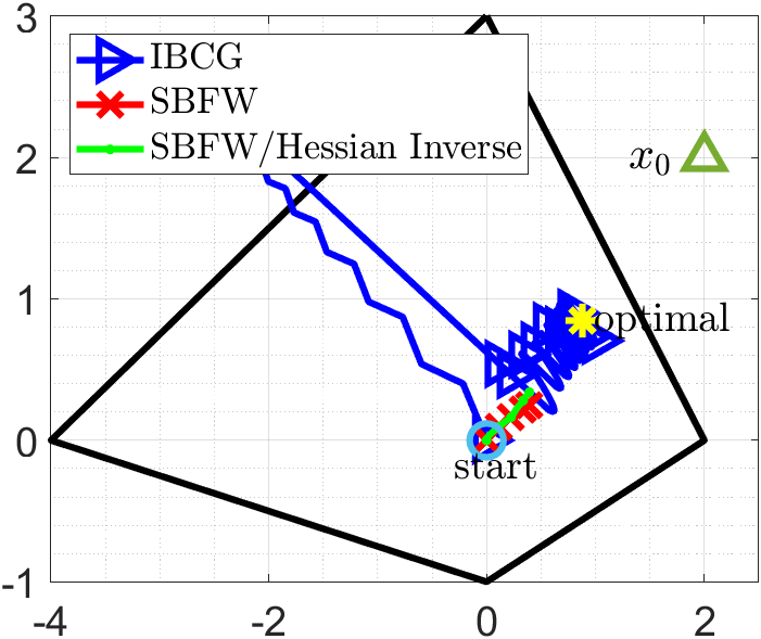
Figure 3: The performance of IBCG (blue) vs SBFW (red) and SBFW with Hessian inverse (green) on Problem 13 when $\mu_{g}=0.1$. Plots from left to right are trajectories of $\theta_{k}$ and $f(\lambda_{k},\theta_{k})-f^{*}$.

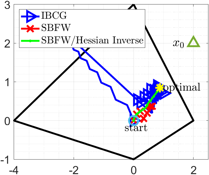
Figure 4: The performance of IBCG (blue) vs SBFW (red) and SBFW with Hessian inverse (green) on Problem 13 when $\mu_{g}=0.1$ and the SBFW parameters are tuned. Plots from left to right are trajectories of $\theta_{k}$ and $f(\lambda_{k},\theta_{k})-f^{*}$.

G.3 Matrix completion with denoising

Dataset Generation. We create an observation matrix $M=\hat{X}+E$. In this setting $\hat{X}=WW^{T}$ where $W\in\mathbb{R}^{n\times r}$ containing normally distributed independent entries, and $E=\hat{n}(L+L^{T})$ is a noise matrix where $L\in\mathbb{R}^{n\times n}$ containing normally distributed independent entries and $\hat{n}\in(0,1)$ is the noise factor. During the simulation process, we set $n=250$, $r=10$, and $\alpha=\|\hat{X}\|_{*}$.

Initialization. All the methods start from the same initial point $\mathbf{x}_{0}$ and $\mathbf{y}_{0}$ which are generated randomly. We terminate the algorithms either when the maximum number of iterations $K_{\mathrm{max}}=10^{4}$ or the maximum time limit $T_{\mathrm{max}}=2\times 10^{2}$ seconds are achieved.

Implementation Details. For our method IBCG, we choose the step-sizes as $\gamma=\frac{1}{4\sqrt{K}}$ to avoid instability due to large initial step-sizes. We tuned the step-size $\eta_{k}$ in the SBFW method by multiplying it by a factor of 0.8, and for the TTSA method, we tuned their step-size $\beta$ by multiplying it by a factor of 0.25.

References

- [ABTR22] Zeeshan Akhtar, Amrit Singh Bedi, Srujan Teja Thomdapu and Ketan Rajawat “Projection-Free Stochastic Bi-Level Optimization” In IEEE Transactions on Signal Processing 70 IEEE, 2022, pp. 6332–6347
- [BMK20] Zalán Borsos, Mojmir Mutny and Andreas Krause “Coresets via bilevel optimization for continual learning and streaming” In Advances in Neural Information Processing Systems 33, 2020, pp. 14879–14890
- [BM73] Jerome Bracken and James T McGill “Mathematical programs with optimization problems in the constraints” In Operations research 21.1 INFORMS, 1973, pp. 37–44
- [Bra20] Jan Brand “A deterministic linear program solver in current matrix multiplication time” In Proceedings of the Fourteenth Annual ACM-SIAM Symposium on Discrete Algorithms, 2020, pp. 259–278 SIAM
- [CXZ23] Lesi Chen, Jing Xu and Jingzhao Zhang “On Bilevel Optimization without Lower-level Strong Convexity” In arXiv preprint arXiv:2301.00712, 2023
- [CSXY22] Tianyi Chen, Yuejiao Sun, Quan Xiao and Wotao Yin “A single-timescale method for stochastic bilevel optimization” In International Conference on Artificial Intelligence and Statistics, 2022, pp. 2466–2488 PMLR
- [CLS21] Michael B Cohen, Yin Tat Lee and Zhao Song “Solving linear programs in the current matrix multiplication time” In Journal of the ACM (JACM) 68.1 ACM New York, NY, USA, 2021, pp. 1–39
- [Dom12] Justin Domke “Generic Methods for Optimization-Based Modeling” In Proceedings of the Fifteenth International Conference on Artificial Intelligence and Statistics, 2012, pp. 318–326
- [FMO20] Alireza Fallah, Aryan Mokhtari and Asuman Ozdaglar “Personalized federated learning with theoretical guarantees: A model-agnostic meta-learning approach” In Advances in Neural Information Processing Systems 33, 2020, pp. 3557–3568
- [FAL17] Chelsea Finn, Pieter Abbeel and Sergey Levine “Model-agnostic meta-learning for fast adaptation of deep networks” In International conference on machine learning, 2017, pp. 1126–1135 PMLR
- [FFSGP18] L. Franceschi, P. Frasconi, S. Salzo, R. Grazzi and M. Pontil “Bilevel Programming for Hyperparameter Optimization and Meta-Learning” In ICML, 2018
- [FFSGP18a] Luca Franceschi, Paolo Frasconi, Saverio Salzo, Riccardo Grazzi and Massimiliano Pontil “Bilevel programming for hyperparameter optimization and meta-learning” In International Conference on Machine Learning, 2018, pp. 1568–1577 PMLR
- [FW56] Marguerite Frank and Philip Wolfe “An algorithm for quadratic programming” In Naval research logistics quarterly 3.1-2 Wiley Online Library, 1956, pp. 95–110
- [GW18] Saeed Ghadimi and Mengdi Wang “Approximation methods for bilevel programming” In arXiv preprint arXiv:1802.02246, 2018
- [GFCACG16] Stephen Gould, Basura Fernando, Anoop Cherian, Peter Anderson, Rodrigo Santa Cruz and Edison Guo “On differentiating parameterized argmin and argmax problems with application to bi-level optimization” In arXiv preprint arXiv:1607.05447, 2016
- [GFPS20] Riccardo Grazzi, Luca Franceschi, Massimiliano Pontil and Saverio Salzo “On the iteration complexity of hypergradient computation” In International Conference on Machine Learning, 2020, pp. 3748–3758 PMLR
- [HJS92] Pierre Hansen, Brigitte Jaumard and Gilles Savard “New branch-and-bound rules for linear bilevel programming” In SIAM Journal on scientific and Statistical Computing 13.5 SIAM, 1992, pp. 1194–1217
- [HWWY20] Mingyi Hong, Hoi-To Wai, Zhaoran Wang and Zhuoran Yang “A two-timescale framework for bilevel optimization: Complexity analysis and application to actor-critic” In arXiv preprint arXiv:2007.05170, 2020
- [Jag13] Martin Jaggi “Revisiting Frank-Wolfe: Projection-Free Sparse Convex Optimization” In Proceedings of the 30th International Conference on Machine Learning, 2013, pp. 427–435
- [JYL21] Kaiyi Ji, Junjie Yang and Yingbin Liang “Bilevel optimization: Convergence analysis and enhanced design” In International Conference on Machine Learning, 2021, pp. 4882–4892
- [JYL20] Kaiyi Ji, Junjie Yang and Yingbin Liang “Provably faster algorithms for bilevel optimization and applications to meta-learning”, 2020
- [Kar84] Narendra Karmarkar “A new polynomial-time algorithm for linear programming” In Proceedings of the sixteenth annual ACM symposium on Theory of computing, 1984, pp. 302–311
- [KZHWWY21] Prashant Khanduri, Siliang Zeng, Mingyi Hong, Hoi-To Wai, Zhaoran Wang and Zhuoran Yang “A near-optimal algorithm for stochastic bilevel optimization via double-momentum” In Advances in neural information processing systems 34, 2021, pp. 30271–30283
- [KT99] Vijay Konda and John Tsitsiklis “Actor-critic algorithms” In Advances in neural information processing systems 12, 1999
- [KKWN23] Jeongyeol Kwon, Dohyun Kwon, Stephen Wright and Robert Nowak “A Fully First-Order Method for Stochastic Bilevel Optimization” In arXiv preprint arXiv:2301.10945, 2023
- [Lan13] Guanghui Lan “The complexity of large-scale convex programming under a linear optimization oracle” In arXiv preprint arXiv:1309.5550, 2013
- [LGH22] Junyi Li, Bin Gu and Heng Huang “A fully single loop algorithm for bilevel optimization without hessian inverse” In Proceedings of the AAAI Conference on Artificial Intelligence 36.7, 2022, pp. 7426–7434
- [LXFZYPUZ18] Renjie Liao, Yuwen Xiong, Ethan Fetaya, Lisa Zhang, KiJung Yoon, Xaq Pitkow, Raquel Urtasun and Richard Zemel “Reviving and improving recurrent back-propagation” In International Conference on Machine Learning, 2018, pp. 3082–3091 PMLR
- [LMYZZ20] Risheng Liu, Pan Mu, Xiaoming Yuan, Shangzhi Zeng and Jin Zhang “A generic first-order algorithmic framework for bi-level programming beyond lower-level singleton” In International Conference on Machine Learning, 2020, pp. 6305–6315 PMLR
- [LVD20] Jonathan Lorraine, Paul Vicol and David Duvenaud “Optimizing millions of hyperparameters by implicit differentiation” In International Conference on Artificial Intelligence and Statistics, 2020, pp. 1540–1552 PMLR
- [MDA15] Dougal Maclaurin, David Duvenaud and Ryan Adams “Gradient-based Hyperparameter Optimization through Reversible Learning” In Proceedings of the 32nd International Conference on Machine Learning, 2015, pp. 2113–2122
- [MD21] Andrew D McRae and Mark A Davenport “Low-rank matrix completion and denoising under Poisson noise” In Information and Inference: A Journal of the IMA 10.2 Oxford University Press, 2021, pp. 697–720
- [MHK20] Aryan Mokhtari, Hamed Hassani and Amin Karbasi “Stochastic conditional gradient methods: From convex minimization to submodular maximization” In The Journal of Machine Learning Research 21.1 JMLRORG, 2020, pp. 4232–4280
- [Moo10] Gregory M Moore “Bilevel programming algorithms for machine learning model selection” Rensselaer Polytechnic Institute, 2010
- [Ped16] Fabian Pedregosa “Hyperparameter optimization with approximate gradient” In Proceedings of the 33nd International Conference on Machine Learning (ICML), 2016
- [RFKL19] Aravind Rajeswaran, Chelsea Finn, Sham M Kakade and Sergey Levine “Meta-learning with implicit gradients” In Advances in neural information processing systems 32, 2019
- [SCHB19] Amirreza Shaban, Ching-An Cheng, Nathan Hatch and Byron Boots “Truncated back-propagation for bilevel optimization” In The 22nd International Conference on Artificial Intelligence and Statistics, 2019, pp. 1723–1732 PMLR
- [SLZ05] Chenggen Shi, Jie Lu and Guangquan Zhang “An extended Kuhn–Tucker approach for linear bilevel programming” In Applied Mathematics and Computation 162.1 Elsevier, 2005, pp. 51–63
- [SJGL22] Daouda Sow, Kaiyi Ji, Ziwei Guan and Yingbin Liang “A constrained optimization approach to bilevel optimization with multiple inner minima” In arXiv preprint arXiv:2203.01123, 2022
- [YH17] Tatsuya Yokota and Hidekata Hontani “Simultaneous visual data completion and denoising based on tensor rank and total variation minimization and its primal-dual splitting algorithm” In Proceedings of the IEEE Conference on Computer Vision and Pattern Recognition, 2017, pp. 3732–3740