Top-Down Network Combines Back-Propagation with Attention

Abstract

Cortical processing, in vision and other domains, combines bottom-up (BU) with extensive top-down (TD) processing. Two primary goals attributed to TD processing are learning and directing attention. These two roles are accomplished in current network models through distinct mechanisms. Attention guidance is often implemented by extending the model’s architecture, while learning is typically accomplished by an external learning algorithm such as back-propagation. In the current work, we present an integration of the two functions above, which appear unrelated, using a single unified mechanism inspired by the human brain. We propose a novel symmetric bottom-up top-down network structure that can integrate conventional bottom-up networks with a symmetric top-down counterpart, allowing each network to recurrently guide and influence the other. For example, during multi-task learning, the same top-down network is being used for both learning, via propagating feedback signals, and at the same time also for top-down attention, by guiding the bottom-up network to perform a selected task. In contrast with standard models, no external back-propagation is used for learning. Instead, we propose a ’Counter-Hebb’ learning, which adjusts the weights of both the bottom-up and top-down networks simultaneously. We show that our method achieves competitive performance on standard multi-task learning benchmarks. Yet, unlike existing methods, we rely on single-task architectures and optimizers, without any task-specific parameters. The results, which show how attention-guided multi-tasks can be combined efficiently with internal learning in a unified TD process, suggest a possible model for combining BU and TD processing in human vision.

1 Introduction

Human cortical processing uses a combination of bottom-up (BU) and top-down (TD) processing streams with bi-directional communication between them. In the visual brain, for example, the BU streams proceed from low-level sensory regions to high-level, more cognitive areas, while in the TD stream, processing flows in the opposite direction. TD processing is believed to serve various functions, including TD attention - guiding perception and cognition according to tasks and contexts (Zagha 2020). Neuroscience evidence suggests that these attention mechanisms can select content via modular representation of knowledge in the cortex (Baars 1997; Dehaene, Lau, and Kouider 2021).

TD processes are involved both in ongoing visual perception, by enhancing or suppressing BU neural responses, as well as in learning processes, by carrying information that is utilized when modifying synapses that control bottom-up processing (Gilbert and Li 2013; Fyall et al. 2017; Lillicrap et al. 2020). Although both BU and TD processing are essential for accurate perception (Manita et al. 2015), most empirical studies have concentrated on examining the processing of sensory information along the BU pathways. As a result, there is currently, a lack of established frameworks that link the mechanisms of cortical feedback pathways with their underlying perceptual and cognitive functions (Zagha 2020; Lillicrap et al. 2020; Kreiman and Serre 2020).

In deep learning networks, TD flow of information plays a central role in learning, by back-propagating feedback error signals (Rumelhart, Hinton, and Williams 1986). However, this is an external computation rather than an integral part of the network. More recently, there has been considerable work towards incorporating TD processing in network models for the purpose of both learning and guiding attention. In modeling top-down attention, the emphasis has been on directing attention to selected locations, context, or tasks showing advantages compared with pure BU models (Pang et al. 2021; Li et al. 2022; Sharifzadeh, Baharlou, and Tresp 2021; Tsotsos 2021; Ronneberger, Fischer, and Brox 2015; Vahdat and Kautz 2020; Ullman et al. 2021; Ben-Yosef et al. 2021; Wang et al. 2019; Shi and Ma 2022; Cheng et al. 2021; Deng et al. 2021; Chen et al. 2020a; Wu et al. 2020; Bian et al. 2020; Zhou et al. 2023; Peng et al. 2023). In the context of learning, the primary focus has been on developing biologically plausible learning algorithms, where learning is an integral part of the network model (Lee et al. 2015; Scellier and Bengio 2017; Akrout et al. 2019; Whittington and Bogacz 2017; Salvatori et al. 2022; Shibuya et al. 2023). Nevertheless, the current implementation of these two functions, learning and attention-guidance, is achieved through unrelated distinct TD mechanisms.

The goal of biological learning models is to gain a deeper understanding of the learning process in the human brain. However, current approaches focus on TD processing solely within the context of learning, neglecting the broader significance of TD streams observed in the brain (Lillicrap et al. 2020; Kreiman and Serre 2020). As a result, unlike the brain where TD streams actively participate in BU processing by influencing the activity state of neurons (Fyall et al. 2017; Manita et al. 2015), the proposed TD mechanisms are used only for learning purposes. Therefore, these TD connections are unable to contribute to guiding attention. This discrepancy highlights a significant gap in the field, as there is currently no existing model that integrates these two functionalities into a unified mechanism. This narrow perspective might limit the ability to accurately model the brain, as it overlooks significant aspects of its functionality.

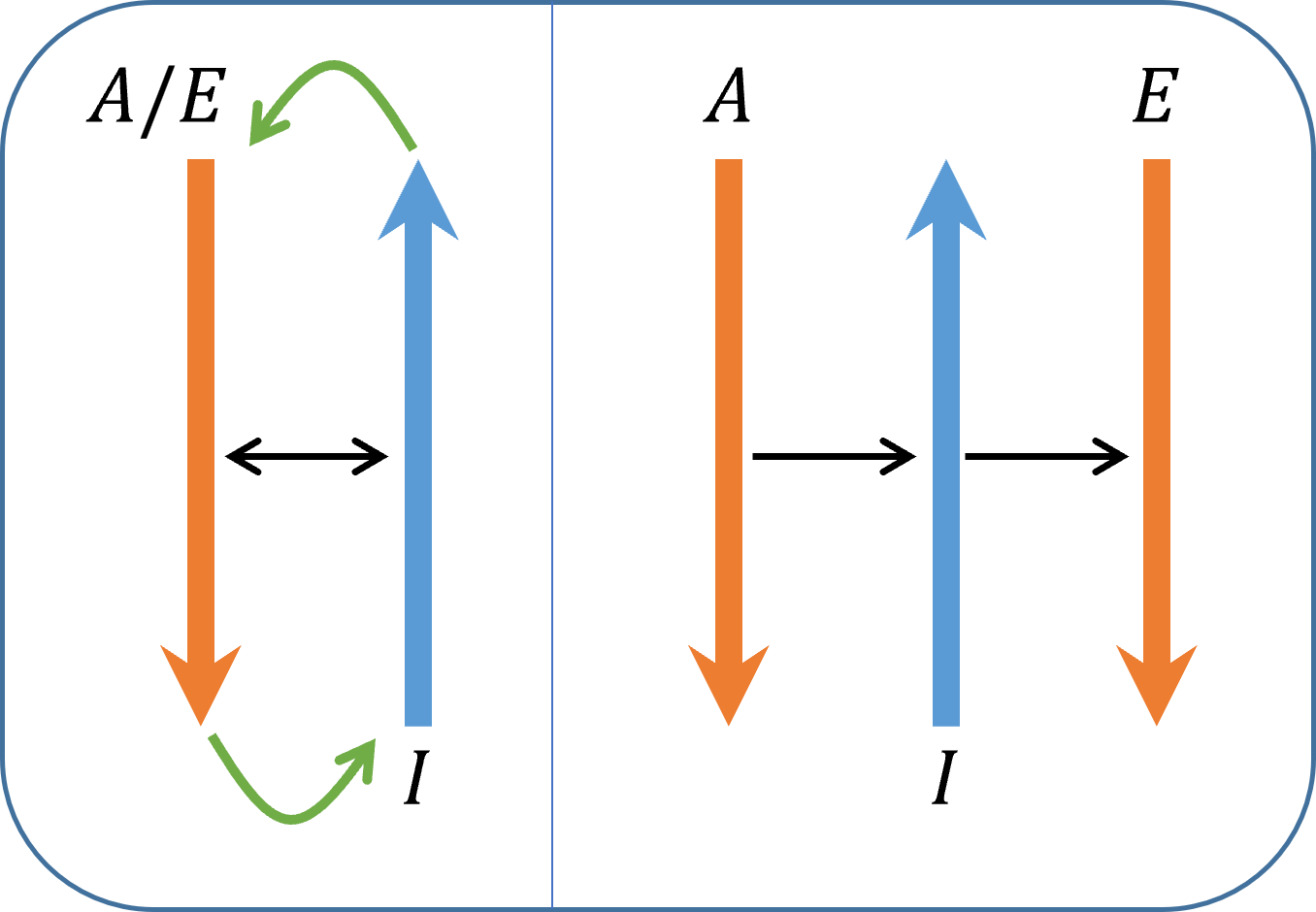
Figure 1: Schematic illustration of the proposed bottom-up (BU) and top-down (TD) approach. The input for each component is indicated by a letter: $I$ marks the input signal (e.g. images in the case of vision), $E$ marks error signals (e.g. loss gradients), and $A$ marks attention signals, e.g. selected object, location, or task. On the left, the general BU-TD approach consists of BU (blue $\uparrow$) and TD (orange $\downarrow$) networks with bi-directional connections. These networks can operate recurrently. A single TD network is used for both propagating down error signals and TD attention ($A/E$), while the BU network handles the processing of input signals ($I$). On the right, this concept is illustrated within a multi-task learning setting, see Fig  3.

We address this gap by proposing a novel BU-TD model that uses a single TD mechanism for both learning and TD attention. This model consists of two symmetric independent networks: a BU network and a TD network. These two networks can communicate through lateral connections to influence the activation of neurons in the other stream, see Figure 1. During learning, the TD network carries error signals and modifies network synapses using a new Counter-Hebbian (CH) learning scheme, which is a modification of the classic Hebbian learning rule (Hebb 2005) that takes into account feedback signals. Interestingly, when the BU and TD weights have similar values, the CH learning algorithm is equivalent to BP for ReLU networks. In addition to learning, the same TD network can naturally be used for TD attention in multi-task learning (MTL) settings, in which a single model learns to solve multiple different tasks, see Figure 1. This model, therefore, offers a new direction for biologically modeling of top-down processing, used for both learning and online processing.

MTL is a natural setting for TD attention, which guides the BU process to perform a selected task. MTL methods have an advantage compared with task-specific networks since they can utilize information shared between different tasks. However, a significant challenge associated with MTL as currently used is negative transfer, which occurs when two tasks have gradients that point in opposing directions, leading to conflicting task gradients (Yu et al. 2020; Liu et al. 2021a). There are two main approaches to MTL: multi-task optimization and multi-task architectures (Crawshaw 2020; Vandenhende et al. 2021). Multi-task optimization focuses on techniques for optimizing a given architecture to fit multiple tasks. These techniques involve modifying the update process to reduce negative transfer and balance the tasks (Yu et al. 2020; Lin, Ye, and Zhang 2021). On the other hand, MTL architectures focus on architectural modifications to construct modular MTL architectures. These architectures decompose a single architecture into multiple sub-modules and selectively combine them for each task to form a ”Mixture of Experts”. Methods differ in the number and complexity of modules (from complex to single neurons), and whether the architecture is pre-determined or learned dynamically (Sun et al. 2020b; Rahaman et al. 2021; Mallya and Lazebnik 2018; Sun et al. 2020a; Kang et al. 2022).

In general, MTL optimization methods require minor architectural modifications but provide limited modularity and introduce complex optimizers. Conversely, MTL architecture methods provide greater modularity but involve significant architectural modifications and rely on an abundance of tricks (Mittal, Bengio, and Lajoie 2022). Our approach is an intermediate one, which offers a modular architecture that can be learned using standard optimizers, without employing any architectural modifications.

Recent work demonstrates that sparse modular architectures lead to better out-of-distribution generalization, scaling properties, learning speed, and interoperability (Mittal, Bengio, and Lajoie 2022; Fedus, Zoph, and Shazeer 2022; Du et al. 2022). Furthermore, there has been a growing interest in the use of functional sparse sub-networks, following the Lottery-Ticket Hypothesis (Frankle and Carbin 2018). The hypothesis suggests that large dense networks contain smaller sub-networks that can match the performance of the full network when training in isolation. This hypothesis has been supported by empirical evidence and was proven under certain conditions (Malach et al. 2020). However, finding such sub-networks is challenging and is an active area of current research (Chen et al. 2021; Morcos et al. 2019; Ramanujan et al. 2020; Tanaka et al. 2020; Yu et al. 2022).

In this paper, we propose to extend this hypothesis suggesting that a sufficiently large network contains multiple overlapping sub-networks, each suitable for a different task. Implying that large network models can actually be perceived as sparse modular architecture. Our work suggests that these sub-networks can be naturally revealed by a top-down process using the same mechanism as for propagating feedback signals. These findings align with the processes observed in the human brain, where a unified TD mechanism is used for both the learning process and the guidance of top-down attention through the selection of sub-modules.

The key contributions of our work are: We propose a novel top-down mechanism that combines learning from error signals with top-down attention. Following earlier work, we offer a new step toward a more biologically plausible learning model. The proposed Counter-Hebbian learning uses a top-down network for propagating feedback signals and a local update rule. In contrast with current learning models, our top-down process can also alter the activity of neurons during the bottom-up forward propagation. We present a novel MTL algorithm that dynamically creates unique task-dependent sub-networks within conventional networks. Unlike standard MTL approaches, this algorithm uses standard optimizers without any architectural modifications or task-specific parameters.

Code for generating BU-TD networks enabling CH learning and MTL is available at https://github.com/royabel/Top-Down-Networks.

2 Related Work

The fields of brain modeling and deep learning have beneficial interactions going in both directions. Artificial neural networks were shown to have intriguing connections with neural networks in the human brain (Khaligh-Razavi and Kriegeskorte 2014; Güçlü and van Gerven 2015; Kriegeskorte 2015; Yamins et al. 2014; Dwivedi et al. 2021). For example, it has been demonstrated that learned neuronal representations are similar across the brain and artificial models (Banino et al. 2018; Whittington et al. 2018; Yamins and DiCarlo 2016; Bersch et al. 2022). The findings suggest that the brain may use computations that bear similarity to those used in deep learning models. Consequently, many researchers are exploring biologically-plausible learning algorithms with the goal of gaining a deeper understanding of the learning process in the human brain.

The back-propagation scheme (Rumelhart, Hinton, and Williams 1986) is the primary algorithm for learning in most deep learning models. It has two basic aspects that are consistent with biological networks: learning by synaptic modification, and feedback signals delivering error information (Lillicrap et al. 2020). However, this algorithm is considered biologically implausible due to several reasons: 1) biological synapses change their connection strength based solely on the activity of the neurons they connect (Whittington and Bogacz 2019). 2) The ’weight transport’ problem: BP demands synaptic symmetry in the forward and backward paths (Grossberg 1987). 3) In BP, feedback connections deliver error signals that do not influence the activity states of neurons, whereas, in the brain, feedback alters neural activity (Lillicrap et al. 2020). 4) The ’update locking’ problem (Jaderberg et al. 2017). 5) The BP algorithm relies on derivatives that require continuous neurons’ output as opposed to biological neurons that fire discrete spikes (Whittington and Bogacz 2019). 6) BP uses signed error signals which require both positive and negative neural activations that appear problematic in the cortex (Lillicrap et al. 2020).

Alternatives to BP is an active area of research and many models have been proposed in an attempt to overcome the aforementioned issues. These alternatives are inspired by biological principles such as Hebb’s plasticity rule (Hebb 2005), which proposes that the brain strengthens synapses between neurons that are co-activated. Even though there is much evidence supporting Hebbian principles in the human brain, it appears that purely Hebbian learning is not sufficient for learning complex tasks (McClelland 2006). Hebbian models often use only the feedforward projections, without an explicit use of the feedback projections. Therefore, integrating feedback information into Hebbian principles may lead to biologically plausible learning algorithms that are capable of learning complex tasks.

Several primary approaches exist for biologically motivated learning algorithms. Energy-based methods, such as Hopfield models and predictive coding methods, aim to reach an equilibrium of an energy function to achieve synaptic updates (Whittington and Bogacz 2017; Scellier and Bengio 2017; Song et al. 2020; Millidge, Tschantz, and Buckley 2022; Laborieux et al. 2021; Salvatori et al. 2022). Target-Propagation methods propagate backward targets instead of gradients (Lee et al. 2015; Bengio 2014; Meulemans et al. 2020; Ahmad, van Gerven, and Ambrogioni 2020; Ernoult et al. 2022; Shibuya et al. 2023). Feedback-Alignment methods propose replacing the symmetric weights used in back-propagation with different weights (Akrout et al. 2019; Lillicrap et al. 2016; Nøkland 2016; Crafton et al. 2019; Launay et al. 2020; Song, Xu, and Lafferty 2021). Forward-only methods, on the other hand, avoid any backward computation (Dellaferrera and Kreiman 2022; Hinton 2022). Additionally, there exist alternative methods that do not fall within the aforementioned categories (Chung 2022; Ororbia et al. 2023). We provide a comprehensive survey that describes the different methods in detail in Appendix  G.

3 The Bottom-UP Top-Down Model

In this section, we introduce the suggested structure of the Bottom-Up (BU) and Top-Down (TD) networks. A BU network with $L$ hidden layers is a function that maps an input vector $x\coloneqq h_{0}$ to an output vector $y$, such that for every layer $0\leq l<L$: the hidden values are defined to be:

$$h_{l+1}\coloneqq\sigma\left(f_{l+1}(h_{0},h_{1},...,h_{l})\right)$$ (1)

The functions $f_{l}$ are linear, and the activation function $\sigma$ is an element-wise function that may be non-linear. A prediction head function $H_{pred}$ maps the last hidden layer $h_{L}$ to the predicted output: $y=H_{pred}(h_{L})$.

For a given BU network, we define a symmetric TD network (denoted with upper bars), to be the reversed architecture network that maps an input vector $\bar{y}$ to an output vector $\bar{x}\coloneqq\bar{h}_{0}$. The TD network is constructed based on the BU architecture as follows: The input (i.e. the prediction error) $\bar{y}$ is mapped to the top-level hidden layer $\bar{h}_{L}$ of the TD network via the TD prediction head: $\bar{h}_{L}=\bar{H}_{pred}(\bar{y})$, and then for every $0\leq l<L$:

$$\bar{h}_{l}\coloneqq\bar{\sigma}\left(\bar{f}_{l+1}(\bar{h}_{L},\bar{h}_{L-1},...,\bar{h}_{l+1})\right)$$ (2)

The TD network satisfies two conditions. First, we restrict $\bar{h}_{l}$ for every $l$ such that $h_{l}$ and $\bar{h}_{l}$ will have the same size (the same number of neurons). Hence, we can define pairs of corresponding neurons by assigning for each BU neuron $h_{l,i}$ in layer $l$, its ’counter neuron’ to be the TD neuron $\bar{h}_{l,i}$. We also use the following notation for simplicity: $\bar{\bar{h}}\coloneqq h$. Additionally, we restrict $\bar{f}_{l}$ to have the same connectivity structure as $f_{l}$, but with the opposite direction: each pair of TD neurons are linked if and only if a link exists between their corresponding BU counter neurons. For example, given a fully connected layer $h_{l}=f_{l}(h_{l-1})=W_{l}h_{l-1}$, the corresponding TD layer $\bar{f}_{l}$ is defined to be also a fully connected layer $\bar{h}_{l-1}=\bar{f}_{l}(\bar{h}_{l})=\bar{W}_{l}\bar{h}_{l}$ such that the shape of the TD weights matrix $\bar{W}_{l}$ is equal to the shape of the transposed BU weights matrix ${W_{l}}^{T}$.

Activation Functions and Biases

The activation functions $\sigma$, $\bar{\sigma}$, may be any element-wise functions. In this work, we focus on two functions. The first is ReLU which is commonly used for neural networks $ReLU(x)\coloneqq(x)_{+}=\begin{cases}x&x>0\\ 0&x\leq 0\end{cases}$. The second is Gated-Linear-Unit (GaLU), which exploits our BU-TD structure by gating according to the counter neurons.

$$GaLU(x)\coloneqq GaLU(x,\bar{x})\coloneqq x\cdot I_{\{\bar{x}>0\}}=\begin{cases}x&\bar{x}>0\\ 0&\bar{x}\leq 0\end{cases}$$ (3)

Where $\bar{x}$ is the counter neuron of $x$, and $I$ is an indicator function.

GaLU has some interesting properties. It introduces lateral connectivity between the BU and TD networks by temporarily turning off neurons based on the values of their counter neurons. As a result, each network can effectively guide its counterpart to operate on a specific partial sub-network. However, it is worth noting that the gradients of this function with respect to the gate $\bar{x}$ are always zero. Additionally, GaLU applies a product of $x$ with the indicator $I_{\{\bar{x}>0\}}$ which is exactly the gradient of the ReLU function: $\frac{\partial}{\partial\bar{x}}ReLU(\bar{x})=I_{\{\bar{x}>0\}}$. This property will be used in section  4 to construct a backward pass that is equivalent to BP.

In this paper, bias terms are omitted to simplify the model. Nevertheless, biases can be represented using additional neurons and weights, as commonly practiced (Ahmad, van Gerven, and Ambrogioni 2020; Lee et al. 2015). This approach enables biases without explicitly using bias terms. In addition, we allow two modes of biases. The first is the standard bias mechanism, in which biases contribute to the output. The second mode is ’bias-blocking’ (Akrout et al. 2019) in which all bias terms are zeroed.

4 Counter-Hebbian Learning

In this section, we formulate the Counter-Hebb learning. Consider a given weights matrix $W$ such that $b=Wa$. The $i,j$-th entry in that matrix, $W^{(t)}_{ij}$, represents the strength of the connection from the neuron $a_{j}$ to the neuron $b_{i}$ at time $t$. Then the update rule is:

$$\Delta W^{(t+1)}_{ij}\coloneqq W^{(t+1)}_{ij}-W^{(t)}_{ij}=\eta\cdot a_{j}\cdot\bar{b}_{i}$$ (4)

where $\eta$ is the learning rate, and $\bar{b}_{i}$ is the counter neuron of $b_{i}$. Note that the rule is applied to all weights including both up-streams and down-streams, resulting in the same update to $W$ and $\bar{W}$, see Figure  2.

There is a strong connection between this rule and the classic Hebb rule. In both cases, the modifications of a synapse (weight) are determined entirely by the activation values of neurons in the network associated directly with the changing synapse. Hebbian plasticity proposes that the synapse between a pre-synaptic neuron and post-synaptic neuron is strengthened when the firing of the pre-synaptic neuron is often followed by the firing of the post-synaptic neuron, within a given time interval (Hebb 2005; Magee and Johnston 1997). In contrast, the Counter-Hebb synaptic modification also depends on the approximate coincidence of two signals, but the post-synaptic cell is replaced by the counterpart neuron. Empirical findings from CA1 hippocampal cells support the existence of such connectivity, offering evidence for synaptic plasticity dependent on the coincidence of two signals from feedforward and feedback sources (Cornford et al. 2019). Through this approach, we effectively incorporate feedback streams, carrying error signals which are valuable for learning, unlike the traditional Hebbian rule (McClelland 2006), see Figure 2.

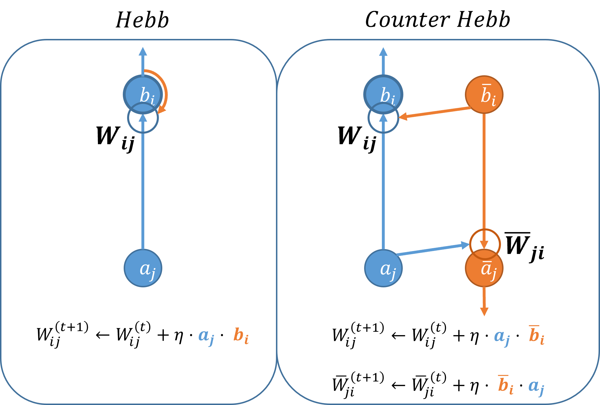
Figure 2: The Counter-Hebb update rule in comparison with the classical Hebb rule. The classical Hebbian plasticity update rule is presented on the left, with a focus on a single upstream synapse $W_{ij}$ (outlined by a circle), connecting a pre-synaptic neuron $a_{j}$ with a post-synaptic neuron $b_{i}$. Neuron $a_{j}$ delivers information directly to the synapse $W_{ij}$, while neuron $b_{i}$ transmits its information through firing that propagates down the dendritic tree to the synapse $W_{ij}$ (orange arrow). Thus, the synapse $W_{ij}$ is updated based on the activity of both associated neurons $a_{j}$ and $b_{i}$ according to the equation shown in the figure. In contrast, the Counter-Hebb update rule, presented on the right, relies on the counterpart downstream (marked in orange) which is connected via lateral connections. It also involves updating a synapse based on the activity of its associated neurons. However, in this case, the signal from $a_{j}$ is combined with the signal from neuron $\bar{b}_{i}$ rather than neuron $b_{i}$. Notably, the resulting Counter-Hebb rule applies an identical update to both $W_{ij}$ and its counter synapse $\bar{W}_{ji}$.

The Learning Algorithm

This section presents the Counter-Hebbian (CH) learning algorithm and discusses some of its biological aspects compared with alternative models. The learning algorithm is described in Algorithm  1. Similar to the back-propagation algorithm, the CH algorithm involves a single forward pass performed by the BU network to compute predictions from an input signal. Subsequently, a single backward pass is conducted using the TD network to propagate error information, and the weights are updated according to the CH update rule.

Algorithm 1 Counter-Hebbian learning

1:  Run the BU network to map the input $x$ to an output $y$ with a non-linear activation function.

2:  Compute error signals.

3:  Run the TD network using the error signals as inputs, in a bias-blocking mode with GaLU (no non-linearity).

4:  Update both the BU and TD parameters according to the Counter-Hebb learning rule.

A special case is when the BU non-linearity is chosen to be the ReLU function, and the computed error signals are the gradients of a loss function with respect to the BU output. In this case, the proposed learning algorithm is equivalent mathematically to the weight-mirroring Feedback-Alignment method (Akrout et al. 2019). However, although the update rule is the same, the implementation of the learning process (e.g. the use of gating) is different. Furthermore, a key distinction is that instead of using a new set of weights exclusively for learning, our model utilizes the TD network for more than this single purpose.

In the scheme above, the following results shown by Akrout et al. (2019), are also applicable to the CH learning algorithm: 1) As training progresses, the BU and TD weights gradually become more symmetric. Moreover, if they are initialized with identical values, their weights would maintain their similarity during learning. This outcome results from the symmetric rule that applies an identical update to both the BU and TD weights. As a result, the CH update rule implicitly constrains the BU and TD weights to be symmetric. 2) Assuming the BU and TD weights are symmetric, the CH learning algorithm is equivalent to back-propagation and the product $a_{j}\cdot\bar{b}_{i}$ in equation  4 is actually the gradient of the loss with respect to $W_{ij}$. Consequently, the derived update effectively implements Stochastic Gradient Descent (SGD). See Appendix  E for a motivation for this equivalence.

While The CH learning algorithm can perform the same exact computation as external BP for standard ReLU networks, it is considered more biologically plausible than BP. CH learning uses a local update rule, in which, like the Hebb rule, the modifications of a synapse are determined entirely by the activation values of neurons in the network associated directly with the synapse. From a connectivity perspective, anatomical and biological evidence supports the existence of top-down streams and lateral connections (Markov et al. 2014), facilitating the communication between neurons in opposite streams. Additionally, it does not suffer from the ’weight transport’ problem (Grossberg 1987).

Compared with alternative models, although many biologically motivated learning algorithms have been proposed, see Section  2, there is a major difference between the current and these alternative models. Previous approaches have focused on the use of feedback streams solely for the purpose of learning. Consequently, while the current feedback mechanisms can modify synaptic weight values, they do not exert any influence on the ongoing activity of the bottom-up streams. As a result, there is currently no link between feedback mechanisms delivering error signals and other known roles of TD processing in perception (Zagha 2020; Lillicrap et al. 2020). To address this limitation, our proposed approach uses a TD network that incorporates both error signal delivery and top-down attention by actively influencing the activity state of bottom-up neurons, see Section  5.

5 Multi-Task Learning

In this section, we describe the second functionality of the same top-down network - controlling top-down attention. In particular, the TD network in our model can guide the BU network to perform multiple tasks by selecting a unique sub-network that fits a given task. In multi-task settings, the objective is to predict an output $y$ given an input $x$ and a task $t$. Therefore, the output of the model must be conditioned on the task. To enable this, our BU-TD structure is designed to have two heads (prediction head, and task head). On the TD stream, the task head $\bar{H}_{task}$ maps a task $t$ to the top-level layer $\bar{h}_{L}$. The TD network can get either a task via the task head or prediction errors via the prediction head but can not get both simultaneously, see Fig 3. To preserve the symmetry, we define also the corresponding BU task head $H_{task}$, which maps the last hidden layer $h_{L}$ to the task. We formulate our MTL algorithm in Algorithm  2, this algorithm comprises of two passes for prediction along with an additional pass for the learning, thereby extending Algorithm  1 with one additional step of selecting the sub-network.

Algorithm 2 Multi-task learning

1:  Run the TD network with task $t$ as input with ReLU, using the task head.

2:  Run the BU network to map the input $x$ to an output $y$ with a composition of ReLU and GaLU.

3:  Compute error signals, i.e. the gradients of a loss $L$ with respect to the BU outputs: $-\frac{\partial L}{\partial y}$

4:  Run the TD network using the error signals as inputs, in a bias-blocking mode with GaLU (no non-linearity).

5:  Update all the weights according to the Counter-Hebb learning rule. (Excluding the task head, see section 6)

Given a task $t$, the TD task head is used to propagate the task representation along the TD network. Since each task activates different patterns, the activated neurons (i.e., with activation value larger than $0$) define a unique task-dependent sub-network. By running the BU network with GaLU activation, we gate the BU computation to propagate the input $x$ along the corresponding BU sub-network. In this manner, the resulting MTL algorithm learns for each task a unique mapping which is conditioned on the task, see Fig  3.

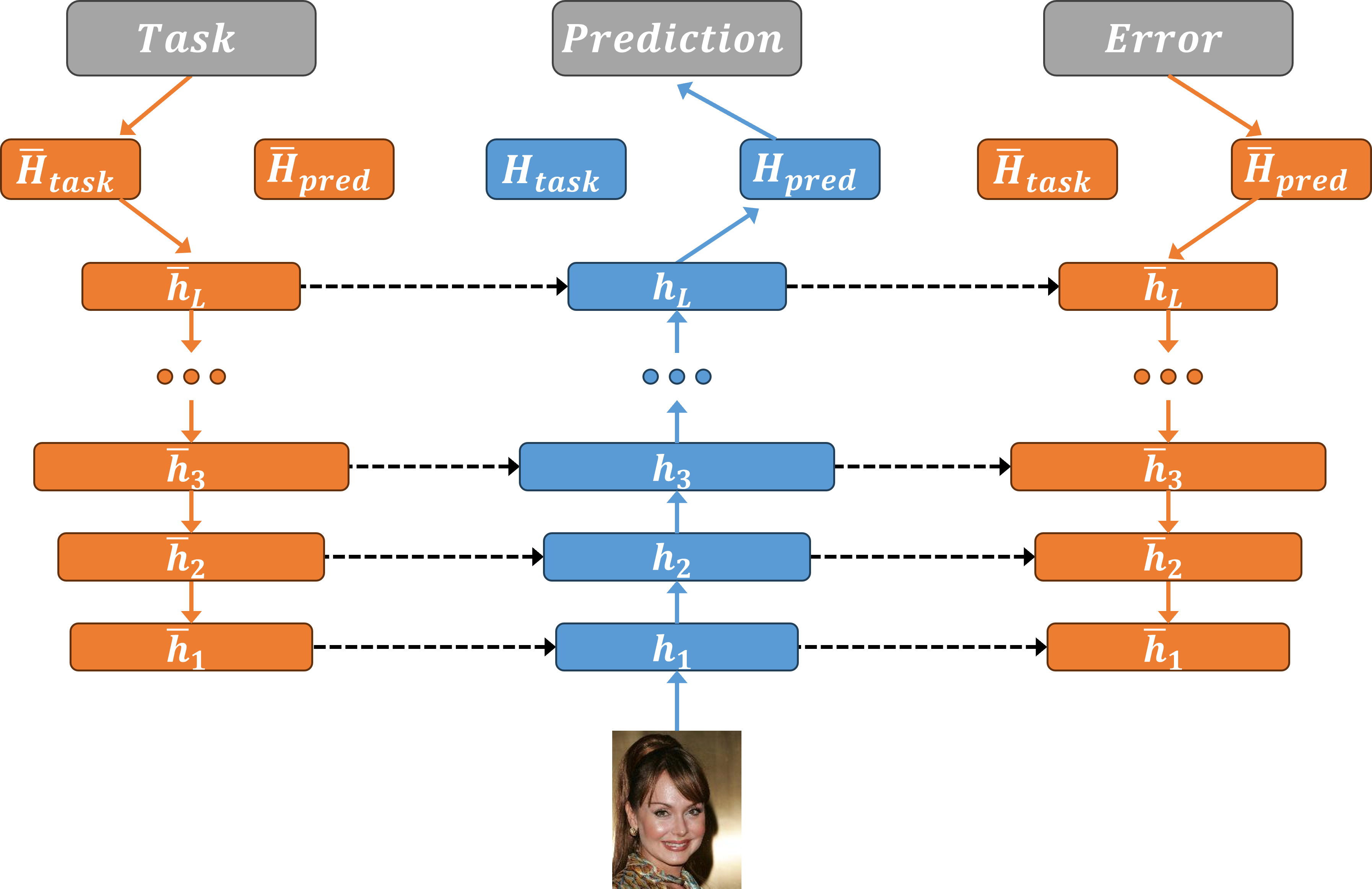
Figure 3: The MTL algorithm comprises of two phases: a TD pass followed by a BU pass for prediction, and another TD pass for learning. The selected task provides input to the TD network via the task head $\bar{H}_{\text{task}}$, and the activation propagates downward attention-guiding signals with ReLU non-linearity. By applying ReLU, the task selectively activates a subset of neurons (i.e. non-zero values), composing a sub-network within the full network. The BU network then processes an input image using a composition of ReLU and GaLU. The GaLU function (denoted with dashed arrows) gates the BU hidden layers $h_{i}$ by their corresponding counter TD hidden layers $\bar{h}_{i}$. As a result, the BU computation is performed only on the selected sub-network. Lastly, the prediction head $H_{\text{pred}}$ generates a prediction based on the top-level BU hidden layer $h_{L}$. For learning, the same TD network is then reused to propagate prediction error signals, starting from the prediction head $\bar{H}_{\text{pred}}$. This computation is performed with GaLU exclusively (no ReLU), thereby permitting negative values. Finally, the ’Counter-Hebb’ learning rule adjusts both networks’ weights based on the activation values of their hidden layers $h_{i}$ and $\bar{h}_{i}$. Therefore, in contrast with standard models, the entire computation is carried out by neurons in the network, and no external computation is used for learning (e.g. Back-Propagation)

Compared with BP, it is important to note that since the gradients of the gating function with respect to the TD activations are always zero, the first TD pass (Algorithm  2, step  1) does not contribute any gradients to the loss function. As a result, gradient-based optimization methods will update only the BU weights, and the TD weights will not be updated. In contrast, our Counter-Hebb learning updates both the BU and TD networks with a symmetric update. It is further important to note that when the BU and TD weights have the same values, this update is equivalent to the BU update derived by standard BP. As a result, it is possible to learn this BU-TD model with gradient-based methods by coupling the BU and TD weights, resulting in sharing a single set of weights across the two networks. In this case, the BP algorithm will update the shared weights, effectively updating both the BU and TD networks with an identical update derived from the gradients of the BU computation (Algorithm  2, step  2). Consequently, the BP algorithm is equivalent to the Counter-Hebbian learning when the BU and TD weights are initialized with similar values (see section  4).

Sharing parameters across the BU and TD networks is computationally appealing. It enables multi-task learning on standard BU architectures. Given a BU network, a symmetric TD network can be constructed using the existing BU parameters without any additional parameters, facilitating multi-task learning by TD guidance without the need for special MTL architectures. Still, it enables a task-dependent sub-network for each task, thereby offering a modular approach using standard architectures and optimizers.

6 Limitations

In this section, we describe the current limitations of our MTL algorithm. The first TD pass is responsible for selecting the task-specific sub-network. However, this computation involves zero gradients, as described in section  5. Therefore, the learning is guided by optimizing the performance of the selected BU sub-network. Additionally, the task head $\bar{H}_{task}$ does not get updated during the learning. As a result, it remains unclear whether the learning is sufficient to bring similar tasks to have similar sub-networks. However, empirical study of the sub-networks and their evolution during learning indicates that the sub-networks are adjusted during the process in a manner that depends on the similarity between tasks, see Appendix  D.

A possible alternative could be to replace the GaLU functions with smooth learnable masks. However, learning such masks appears to raise biological issues, and at the same time, the proposed MTL algorithm appears empirically sufficient to achieve competitive performance. Another direction could be leveraging large pre-trained models, such as vision-language models, for creating task embedding, rather than learning the embedding by the BU-TD network itself.

In addition, although the model has some basic aspects of cortical-like structure, future work will be needed to examine biologically plausible models of different aspects such as the cross-streams gating, the simplified correspondence between a neuron and its counter-neuron, and others.

7 Empirical Results

In this section, we evaluate our BU-TD model, learned via Counter-Hebbian learning, on two commonly used MTL benchmarks, the Multi-MNIST (Sabour, Frosst, and Hinton 2017) dataset, and the CelebA (Liu et al. 2015) dataset. Our goal is not to demonstrate the superiority of our model in terms of performance but to show that a single top-down mechanism is capable of performing well two different functions: learning and directing attention.

In the experiments, we started from random symmetric weights, i.e. the BU and TD networks are initialized with identical weights. From the results shown by Akrout et al., it follows that the use of the Counter-Hebb scheme is guaranteed to converge to symmetric weights, and then remain symmetric. Our own experiments show that in the more realistic case of a noisy update, where the BU and TD weight adjustments are not identical, the weights remain sufficiently close, with no degradation in performance. However initial convergence of the model can require long training, beyond the training on a small number of tasks as in our experiments, see Appendix  C. In addition, unlike the baselines, our model uses a single decoder for all the tasks, resulting in zero task-specific parameters. Therefore, we have also examined the performance of the model when utilizing multiple-decoders - a separate decoder for each task.

The Multi-MNIST dataset contains images of two overlayed digits, where the task indicates whether to classify the left or the right digit. Similar to previous work (Kurin et al. 2022), our BU network employs a simple architecture composed of $2$ convolutional layers followed by a single fully-connected layer and ReLU non-linearity, along with an additional fully-connected layer as the decoder. To support the BU-TD structure, we replace all max-pool layers with strided convolution layers, to gain a similar effect. Note that we slightly increased the number of channels in each convolution layer. Yet, since our model uses only sparse sub-networks for the prediction, its actual size is effectively much smaller compared to the baselines, see Appendix  D.

The CelebA dataset is more challenging, comprising of headshots of celebrities along with the indication of the presence or absence of 40 attributes. Each task is a binary classification problem for an attribute. As done in previous work (Kurin et al. 2022), we employ an encoder-decoder architecture, where the encoder is a ResNet-18 (He et al. 2016) (without the final layer) with batch normalization layers (Ioffe and Szegedy 2015), and the decoder is a single linear layer. Additionally, we remove the last average pooling layer to support the symmetric BU-TD structure.

We compare our approach with current state-of-the-art MTL optimization methods, as reported by Kurin et al. (2022). These comparisons make it possible to compare directly different methods on similar architectures and settings. Similar to previous work, we train the model for $100$ epochs on the Multi-MNIST data set and $50$ epochs on the CelebA dataset. See Appendix  B for the full details of the architecture and hyper-parameters.

The results, presented in Table  1, show that the proposed model incorporates successfully the two different TD functions, directing attention, and internal learning, i.e. using the network itself for learning instead of external BP. The BU-TD model achieves competitive performance compared with leading state-of-the-art methods. See Appendix  B for more details and an analysis of the results.

Method	Multi-MNIST	CelebA
Unit. Scal. (2022)	94.76 $\pm$ 0.44	90.90 $\pm$ 0.08
IMTL (2021b)	94.87 $\pm$ 0.25	90.93 $\pm$ 0.08
MGDA (2018)	94.78 $\pm$ 0.20	90.22 $\pm$ 0.10
GradDrop (2020c)	93.47 $\pm$ 1.30	90.98 $\pm$ 0.03
PCGrad (2020)	94.79 $\pm$ 0.36	90.93 $\pm$ 0.11
RLW Diri. (2021)	94.30 $\pm$ 0.30	90.99 $\pm$ 0.08
RLW Norm. (2021)	93.99 $\pm$ 0.89	90.95 $\pm$ 0.10
Ours	93.09 $\pm$ 0.57	89.51 $\pm$ 0.21
Ours (multi-decoder)	93.86 $\pm$ 0.49	89.69 $\pm$ 0.12

Table 1: MTL results: mean and 95% confidence interval of the avg. task test accuracy (in percentages) across 10 runs for Multi-MNIST and 5 runs for CelebA. The results of the BU-TD model that uses a TD stream for both learning and attention guidance are competitive with state-of-the-art MTL methods, as reported in Kurin et al..

In addition, the proposed method may offer some useful computational properties. The derived task-dependent sub-networks exhibit sparsity, resulting in only a portion of the model that is used during inference, see Appendix  D. Consequently, after the training, we can omit the unused parts of the model, resulting in a compact representation of the model, which is efficient both in terms of computation and memory. Furthermore, the compactness indicates of the capacity of the model to accommodate a larger number of tasks within the same network. Additionally, since the proposed method facilitates training via single-task optimizers, it can enhance learning efficiency. In contrast to MTL optimizers which require per-task gradients, thereby iterating over all possible tasks for each instance, a standard single-task optimizer enables random task sampling per instance without compromising performance. For example, training on CelebA could lead to a reduction of 40 times fewer instances, and evaluating our model on Multi-MNIST with all tasks per instance yields a test accuracy of $93.87\pm 0.38$.

8 Conclusion

In this paper, we propose a novel bottom-up (BU) top-down (TD) model, that combines a conventional BU architecture with a symmetric counter TD network. Extending Akrout et al., this is the first full demonstration of a complete model that performs accurate back-propagation by a TD network. Unlike previous learning models, this TD network can also direct attention by participating in BU processing, as observed in the cortex. We further propose a Counter-Hebbian learning process that modifies the classic Hebbian learning, by combining a pre-synaptic signal with a signal coming from the appropriate counter stream. We have demonstrated that this BU-TD model learned via Counter-Hebb learning achieves competitive results on standard MTL benchmarks. These findings suggest a potential model for combining BU and TD processing within human vision.

It may be possible to test the existence of counter-Hebb learning biologically by the controlled activation of selected layers. For example, cortical layer 3B receives feedforward connections from layer 4 and feedback connections from layer 2/3A (Markov et al. 2014). The counter-Hebbian model predicts that it will be possible to modify the forward synapses from layer 4 to layer 3B by simultaneous activation of the two inputs.

On a general level, it may be noted that the BU-TD model and recent vision-language (VL) models share a similar general structure composed of two streams, a visual stream and a non-visual one, which can guide the visual stream, depending on the current goal. The human brain excels at combining visual and cognitive information in visual perception, and therefore the combination of instructed VL models and principles from human processing can offer a promising direction for future studies.

Appendix A Datasets

Multi-MNIST

Multi-MNIST, introduced by (Sabour, Frosst, and Hinton 2017) and modified by Sener and Koltun (2018), is a simple two-task supervised learning benchmark dataset constructed by uniformly sampling two overlayed MNIST (LeCun et al. 1998) digits. One digit is placed in the top-left corner, while the other is in the bottom-right corner. Each of the two overlaid images corresponds to a 10-class classification task. We generated the dataset using the code provided by Kurin et al. (2022), which samples the training set from the first 50,000 MNIST training images, and the test set from the original MNIST test set. We omitted the validation set, and the hyper-parameters were tuned based solely on the training set.

CelebA

The CelebA dataset (Liu et al. 2015) (with standard training, and test splits) comprises more than 200,000 face images of celebrities along with annotations for 40 attributes, such as the presence of eyeglasses, gender, smiling, and more. Within the context of Multi-Task Learning research, it is frequently approached as a 40-task classification challenge, where each task involves binary classification for one of the attributes.

Appendix B Experimental Settings

All the experiments were conducted using either NVIDIA RTX 6000 GPU or NVIDIA RTX 8000 GPU. For the Multi-MNIST dataset, a single NVIDIA RTX 6000 GPU was used. In the case of the CelebA dataset, either a single NVIDIA RTX 8000 GPU or two NVIDIA RTX 6000 GPUs were used.

In contrast to the baseline methods, we do not use any learning ’tricks’ such as dropout layers, early stopping, regularization, or special MTL optimizers (Kurin et al. 2022; Mittal, Bengio, and Lajoie 2022). Instead, our model is trained straightforwardly using the Adam optimizer (Ruder 2016). Some of the experiments were optimized via the standard back-propagation implementation of Pytorch (Paszke et al. 2017), while others were optimized via the proposed Counter-Hebb learning rule. In the latter, we still use standard Pytorch optimizers, but we replace the gradients with the computed Counter-Hebb update values. These values were fed to the optimizers instead of gradient values.

Since MTL optimizers require per-task gradients, the baseline experiments involve iterating over all potential tasks for every instance during the learning process. However, employing a standard single-task optimizer for more efficient learning by randomly sampling a task for each instance. Consequently, unless specified otherwise, in our experiments, we randomly sample a single task for each training instance. For example, training on the CelebA dataset involves using 40 times fewer instances

Additionally, unlike the baseline methods that require a separate decoder for each task, our method enables a single unified decoder for all the tasks, leading to no architectural modifications and zero task-specific parameters. Thus, unless noted otherwise, our method makes use of a single decoder for all the tasks.

Another distinction from the baseline methods is that we do not use a validation set. As a result, we do not use an early stopping mechanism, and report the final results obtained from the last epoch which might introduce some noisiness. Furthermore, all hyper-parameters were lightly tuned based solely on the training set.

Multi-MNIST Settings

Similar to the baseline experiments conducted in (Kurin et al. 2022), our BU network employs a simple architecture composed of $2$ convolutional layers followed by a single fully-connected layer and ReLU non-linearity, along with an additional fully-connected layer as the decoder. Each convolution layer includes $64$ channels, and a $5\times 5$ kernel (a single stride and no padding). Similar to the baseline, the last fully connected layer size is $50$. Additionally, to support the BU-TD structure, we replace all max-pool layers with strided convolution layers. The strided convolution layer includes the same number of channels but only $3\times 3$ kernel size with stride of $2$.

The standard Adam optimizer (Ruder 2016) was used to optimize the Cross-Entropy loss without any regularization, as opposed to the baseline. Similar to the compared methods, we trained for $100$ epochs with an exponential learning rate decay with $\gamma=0.95$. The initial learning rate was $5\cdot 10^{-4}$, and the batch size $64$. We have chosen the learning rate from $[0.005,0.001,0.0005,0.0001]$ based on the convergence rate on the train set.

We have conducted experiments on our BU-TD model trained using the Counter-Hebbian learning algorithm across the following configurations:

1. symmetric weights, where the weights of the BU and TD networks are initialized with identical values. Since the Counter-Hebb learning preserves this symmetry throughout the entire learning, we can implement it by sharing a single set of parameters for the two networks. As discussed in Section  5, this is equivalent to learning via standard back-propagation under the constraint of symmetric BU and TD weights.

2. multi-decoders, where there is a separate decoder for each task (and symmetric weights).

3. all tasks, where instead of randomly sampling a task for each training instance, we iterate over all the possible tasks for every instance (and symmetric weights + multi-decoders).

4. asymmetric weights, where the weights of the BU and TD networks are initialized with different values. In this case, the weights become gradually similar during training, due to the symmetric update, see Section  4. Similar to previous work (Akrout et al. 2019), we add a weight decay term of $0.05$.

5. weak symmetric, where we initialize the weights of the BU and TD networks with the same values, but we introduce noise to the Counter-Hebb update. This simulates a more realistic case of a noisy update, where the BU and TD weight adjustments are not identical. Therefore, the weights do not maintain an exact symmetry during the learning but remain sufficiently close. Starting close to symmetric weights is a realistic assumption, as initiating from asymmetric weights will also lead to approximately symmetric BU and TD weights after a sufficient number of updates, see Section  4. The noise is introduced by multiplying the outcome of the update rule by a noise factor that is randomly sampled from a $\mathcal{N}(1,\,0.01)$ distribution.

CelebA Settings

As done in previous work (Kurin et al. 2022), we employ an encoder-decoder architecture, where the encoder is a ResNet-18 (He et al. 2016) (without the final layer) with batch normalization layers (Ioffe and Szegedy 2015), and the decoder is a single linear fully-connected layer with a single neuron output for binary classification. Additionally, we remove the last average pooling layer to support the symmetric BU-TD structure.

Batch normalization operates without reliance on learnable parameters, instead utilizing aggregated statistics such as the mean activation value of neurons across multiple iterations. Consequently, we implement distinct batch normalization for the BU and TD networks, with each network gathering statistics relevant to its own operations.

The standard Adam optimizer (Ruder 2016) was used to optimize the Binary-Cross-Entropy loss without any regularization. Similar to the compared methods, we trained for $50$ epochs with an exponential learning rate decay with $\gamma=0.95$. The initial learning rate was $5\cdot 10^{-4}$ which is chosen from $[0.005,0.001,0.0005,0.0001]$ based on the convergence rate on the train set. The batch size is slightly smaller than the baselines in order to fit the GPU memory, and is set to $100$ when the BU and TD networks share the same set of weights, and $64$ otherwise.

We have conducted experiments on our BU-TD model trained using the Counter-Hebbian learning algorithm across the following configurations:

1. symmetric weights, where the weights of the BU and TD networks are initialized with identical values. Since the Counter-Hebb learning preserves this symmetry throughout the entire learning, we can implement it by sharing a single set of parameters for the two networks. As discussed in Section  5, this is equivalent to learning via standard back-propagation under the constraint of symmetric BU and TD weights.

2. multi-decoders, where there is a separate decoder for each task (and symmetric weights).

3. asymmetric weights, where the weights of the BU and TD networks are initialized with different values. In this case, the weights become gradually similar during training, due to the symmetric update, see Section  4. Similar to previous work (Akrout et al. 2019), we add a weight decay term of $0.05$.

Appendix C Results

Multi-MNIST Results

Statistics of the average task test accuracy obtained from the last epoch (no early stopping) with $10$ repetitions are reported in table 2. We compare the BU-TD model across multiple configurations, as described in Appendix  B. In addition, we plot the test results during the training process, sampled every 5 epochs, in Figures  4,  5.

Method	Multi-MNIST Test Accuracy
symmetric weights	93.09 $\pm$ 0.57
multi-decoders	93.86 $\pm$ 0.49
all tasks	93.87 $\pm$ 0.38
asymmetric weights	71.28 $\pm$ 13.81
weak symmetric	93.33 $\pm$ 0.54

Table 2: Multi-MNIST results: mean and 95% confidence interval of the avg. task test accuracy (in percentages) across 10 runs. See Appendix  B for details

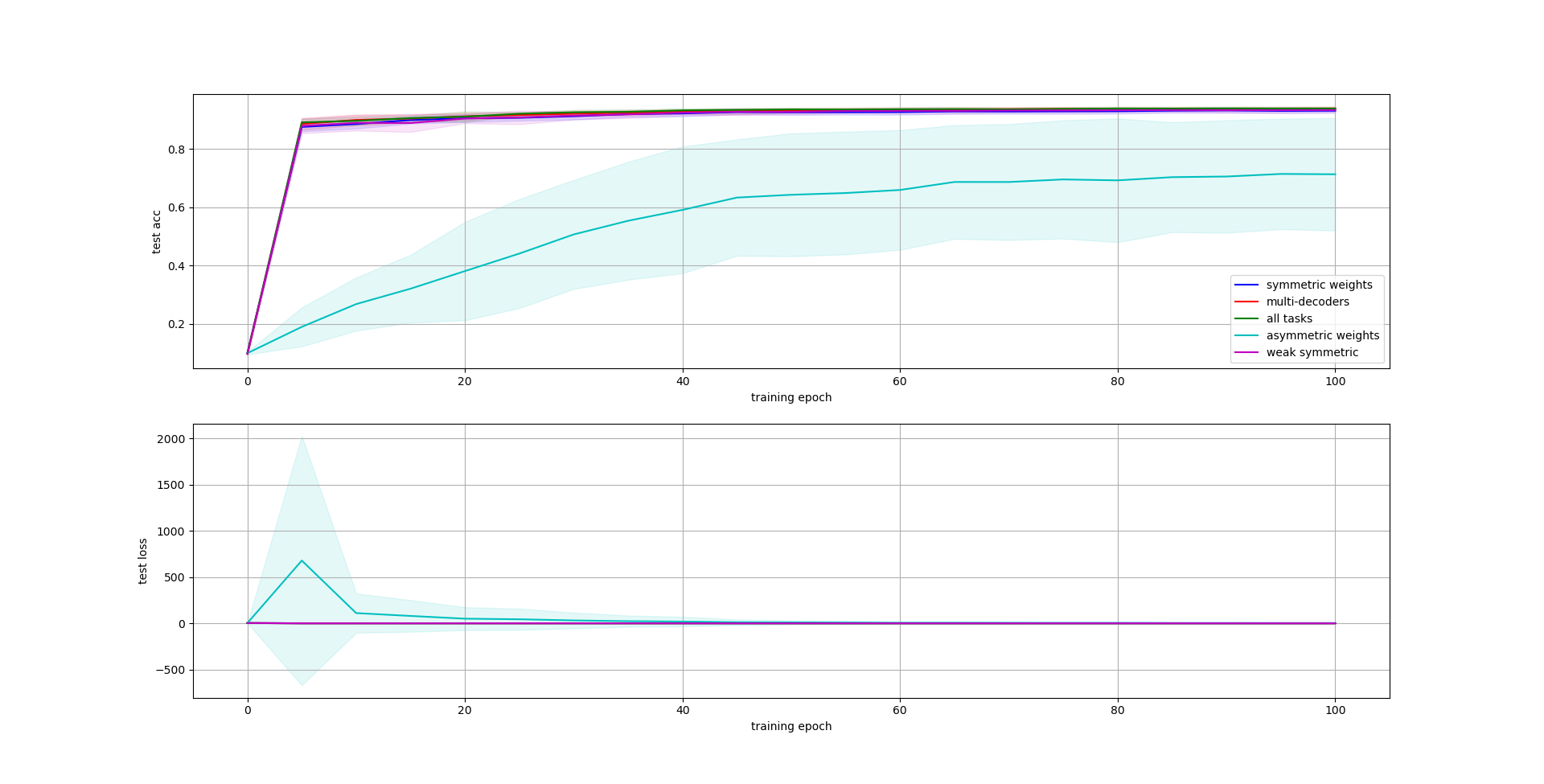
Figure 4: Multi-MNIST results: mean and std of the average task accuracy and loss on the test set per training epoch (sampled every 5 epochs).

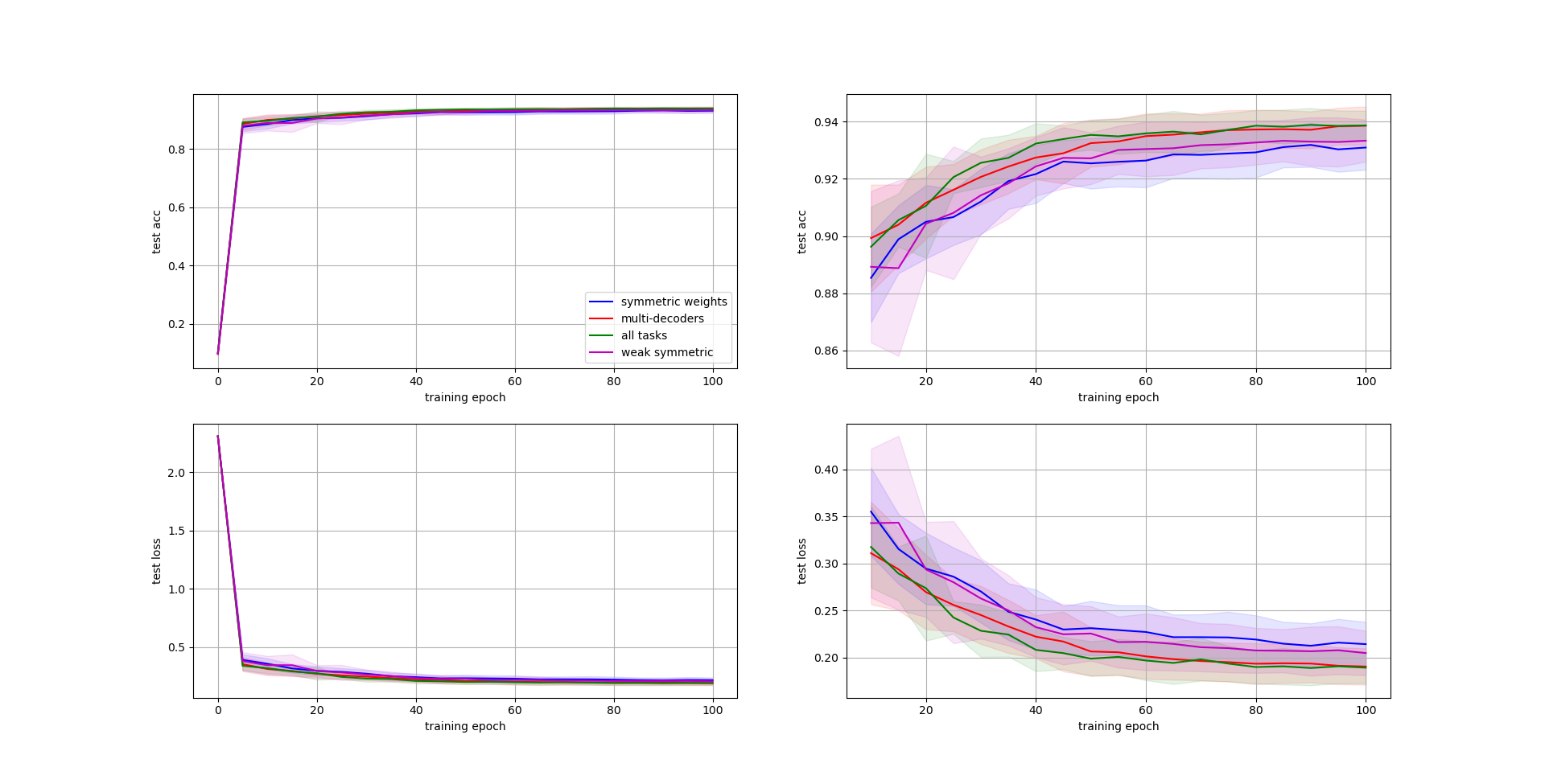
Figure 5: Multi-MNIST results: mean and std of the average task accuracy and loss on the test set per training epoch (sampled every 5 epochs). Within this figure, we omit the results of the asymmetric model due to being far from the other models. This allows for clearer observation of the distinctions among the remaining models. Additionally, on the right, presented the results starting from the 10th epoch.

The results show that the proposed model successfully incorporates the two different TD functions, directing attention, and internal learning, i.e. using the network itself for learning instead of external BP. The BU-TD model, learned via the Counter-Hebbian learning with symmetric weights, consistently converges towards a competitive solution compared with state-of-the-art MTL methods, despite using the same mechanism for both learning and task guidance. Unlike the compared MTL methods, the BU-TD model requires neither multiple decoders nor iterating over all the tasks for each training instance, however, the results show that adding multiple decoders, as done in previous work, slightly increases the performances. Still, iterating over all the tasks does not have an impact.

In the more realistic case of non-symmetric BU and TD weights, it is shown in Fig  4 that when the BU and TD weights are initialized far from symmetric values, the initial model performs badly. However, as the learning progresses, the symmetric update rule pushes the weights to approach symmetry, and the performances start to converge to much higher than chance. However, when the BU and TD weights are initialized symmetrically, but noise is added to the update rule, resulting in non-exact symmetry, the results are on par with the symmetric weight model (which is equivalent to BP).

Asymmetric Weights

From the results shown by Akrout et al., it follows that the use of the Counter-Hebb scheme is guaranteed to converge to symmetric weights, and then remain symmetric. However initial convergence of the model can require long training, beyond the training on a small number of tasks as in our experiments. Moreover, we demonstrate that attaining convergence to symmetric weights by itself does not suffice to yield favorable outcomes. This is evidenced by the model’s inability to attain high performance, even when the weights approximate symmetry by the end of training. This mirrors the significance of initialization techniques in Back-Propagation in general.

We hypothesize that the process of simultaneously learning numerous tasks, which is plausible in human learning, can lead to the convergence of ”good” symmetric weights. The rational is that in our case, the relevant sub-networks constitute only a portion of the model that is being used during the learning. Engaging in the learning of numerous tasks prompts the activation of the complete network model, with updates originating from diverse sources that can balance each other.

The convergence of the BU and TD to be symmetric, regardless of their initial state, enables simulating a mature network model by initialization of nearly symmetric weights from the beginning. This weak symmetry will be maintained through the symmetric update rule. We accomplish this by initializing with symmetric weights and incorporating noise into the update rule, leading to an approximation of symmetry from the second learning iteration onward. This scenario of weakly symmetric weights yields performances that are on par with the case of the symmetric weight, as shown in Figure  5.

CelebA Results

Statistics of the average task test accuracy obtained from the last epoch (no early stopping) with $5$ repetitions are reported in table 3. We compare the BU-TD model across multiple configurations, as described in Appendix  B. In addition, we plot the test results during the training process, sampled every 5 epochs, in Figures  6,  7.

Method	CelebA Test Accuracy
symmetric weights	89.51 $\pm$ 0.21
multi-decoders	89.69 $\pm$ 0.12
asymmetric weights	79.25 $\pm$ 1.63

Table 3: CelebA results: mean and 95% confidence interval of the avg. task test accuracy (in percentages) across 5 runs. See Appendix  B for details

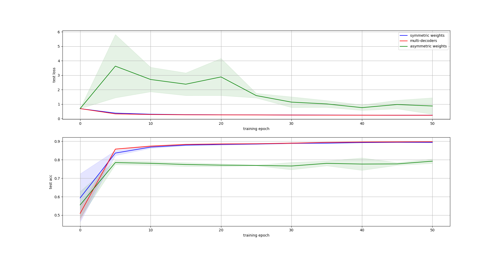
Figure 6: CelebA results: mean and std of the average task accuracy and loss on the test set per training epoch (sampled every 5 epochs).

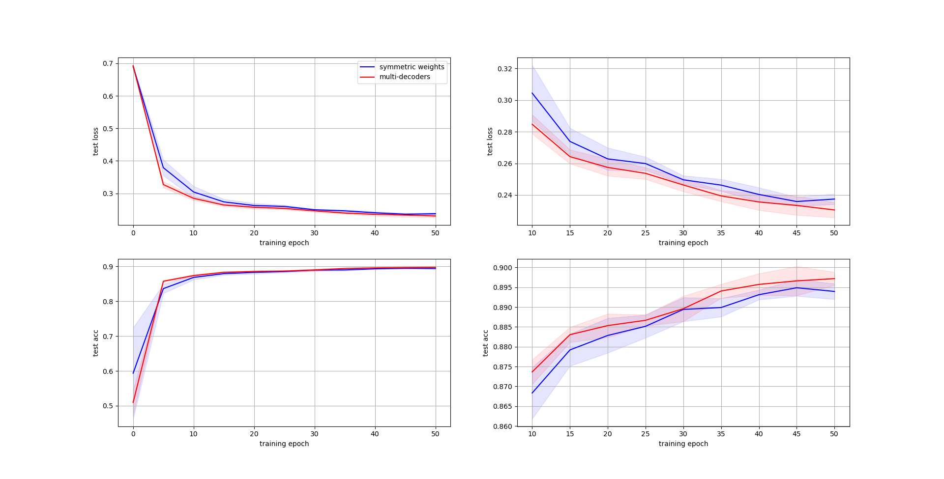
Figure 7: CelebA results: mean and std of the average task accuracy and loss on the test set per training epoch (sampled every 5 epochs). Within this figure, we omit the results of the asymmetric model due to being far from the other models. This allows for clearer observation of the distinctions among the remaining models. Additionally, on the right, presented the results starting from the 10th epoch.

The results on the CelebA dataset, which is more challenging are consistent with the Multi-MNIST results, demonstrating the BU-TD model’s ability to scale and solve complex tasks through Counter-Hebb learning.

Appendix D Sub-Networks Analysis

In our experiments, the model has exhibited the capability to solve multiple tasks by assigning a distinct task-specific sub-network for each task. In this section, we analyze the resulting sub-networks focusing on the Multi-MNIST experiment, where two tasks: ”left” and ”right” are involved. For the purpose of this analysis, we have evaluated a BU-TD model with symmetric weights and a single decoder. Our analysis shows the characteristics of the different sub-networks learned by the model and how they evolved during the learning process. Specifically, we have extracted for each task its corresponding sub-network every 3 epochs. Then we evaluated the size of the sub-networks and examined the level of overlap between them. The analysis is presented in Fig  8. The findings collectively provide insights into the learning dynamics of the model and its ability to develop task-specific representations.

From the figure, several findings can be drawn:

• Dynamic Nature of Sub-Networks: The sub-networks exhibit changes throughout the learning process, indicating that the model adapts and refines its sub-networks representations. This adaptation occurs especially in the earlier epochs of the training.

• Sparsity in Sub-Networks: A notable characteristic of the sub-networks is their sparsity (row 1)- a small percentage of active neurons. The percentage of active neurons drastically decreases at the early iterations until reaching a plateau. The level of sparsity is lower at the first layer as it represents the image signal and needs to capture a large number of pixels.

• Fixed top-level hidden layer: The top-level hidden layer is obtained by passing the task via the task head function. Since we do not update the task head during the training, This layer remains fixed during the learning.

• Similarity Between Sub-Networks: Despite the sparsity of the sub-networks, they demonstrate some degree of similarity (row 2). This outcome is likely due to the major correlation between the ”left” and ”right” tasks, as both tasks aim to identify one out of the same ten digits. The first hidden layer (layer 0) exhibits a degree of similarity, likely arising from the overlap between the two digits. The following hidden layer (layer 1) shows the least similarity. The similarity then increases as moving deeper into the network. A possible explanation could be that early layers focus on the low-level image features at different image locations (left/right), while deeper layers focus on the high-level features for the classification of the identified digit.

The results show that the sub-networks are adjusted during the process, their separation can change at different layers and can depend on the similarity of the tasks.

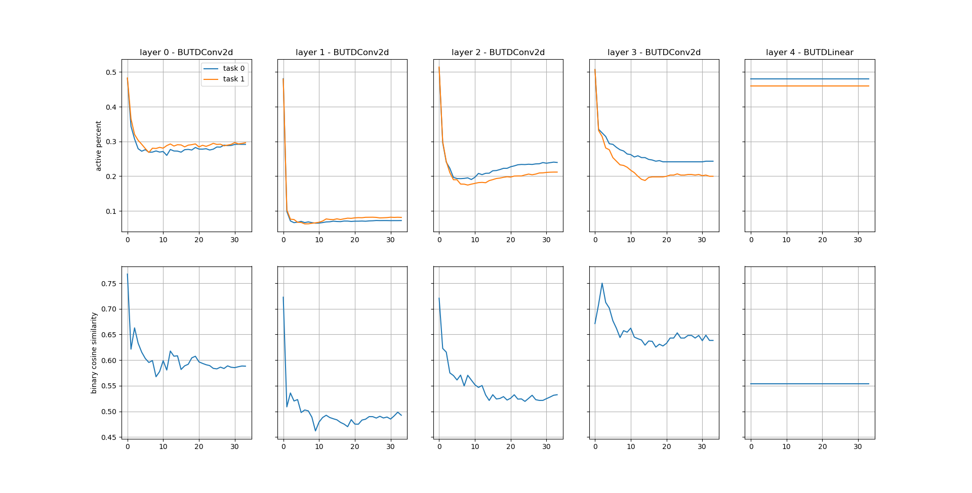
Figure 8: Analysis of the different sub-networks learned by the model and how they evolved during the learning process. We sampled the task-dependent sub-networks for each task Every 3 epochs during learning the Multi-MNIST data set. The columns in the figures represent the different hidden layers in the network, ordered from the first hidden layer on the left to the top hidden layer on the right. The X-axis of all figures represents the epochs during training. The first row shows the percentage of neurons that are being used in each sub-network for every layer. The second row shows the cosine similarity between the binary masking vectors of the two tasks, where 1 indicates an active neuron that is being used in the sub-network and 0 denotes an inactive one.

Appendix E Motivation: Back Propagation - Counter-Hebbian learning

In this section, we give a motivation for the relation between the proposed Counter-Hebbian learning and Back-Propagation (BP). Back-Propagation is a key component of current learning algorithms for artificial neural networks, and modern deep learning models are typically optimized using end-to-end BP and a global, supervised loss function (LeCun, Bengio, and Hinton 2015). BP is an efficient algorithm to compute gradients, designed especially for deep neural networks (Rumelhart, Hinton, and Williams 1986). The algorithm uses the chain rule to back-propagate error signals through the network, thus computing the gradients of a loss function $L$ with respect to all parameters with a single backward pass.

Given a deep architecture, such that in each layer $l$, for $1\leq l\leq L$, the forward pass behaves according to:

$$h_{l}=f_{l}(h_{l-1})=\sigma(W_{l}h_{l-1})$$ (5)

Where $W_{l}$ is the weights parameters of layer $l$, and $\sigma$ is a non-linear element-wise function. Then, the backward pass propagates error signals $\delta$ through the network from the output layer according to:

$$\delta_{l-1}\coloneqq\frac{\partial f_{l}}{\partial h_{l-1}}\delta_{l}=\sigma^{\prime}(h_{l-1})W_{l}^{T}\delta_{l}$$ (6)

Where the initial $\delta$ values, that correspond to the output layer, are the derivative of the loss with respect to the output layer: $\delta_{L}=\frac{\partial\text{Loss}}{\partial h_{L}}$. This definition of $\delta$ enables an easy way to compute the gradients with respect to each parameter:

$$\frac{\partial L}{\partial W_{l}}=\delta_{l}h_{l-1}^{T}$$ (7)

In our BU-TD model, assuming that at initialization, the weights of the TD network were set to be the transposed BU weights. Then, our learning algorithm as described in section  4 can reformulate the exact BP computation for ReLU networks using the TD network, by choosing the inputs to the TD network to be the gradients of the loss function with respect to the BU output.

Under these configurations, the TL process done in step 3 makes the exact same computation as BP. Therefore, the TD neurons’ value contains information related to the gradients, and we obtain exactly the update derived from SGD.

By our construction, we get that $\delta_{l}=\bar{h}_{l}$. This is simply due to the fact that the TD GaLU operation is equivalent to multiplication with the derivatives of the BU ReLU function. Therefore, we get:

$$\bar{h}_{l-1}\coloneqq\text{GaLU}(W_{l}^{T}\bar{h}_{l})=\text{ReLU}^{\prime}(h_{l-1})W_{l}^{T}\bar{h}_{l}$$ (8)

As a result, the update derived from our CH learning is equivalent to BP and also performs SGD:

$$\Delta W_{l}=-\eta\nabla\text{Loss}(W_{l})=-\eta\delta_{l}h_{l-1}^{T}=-\eta\bar{h}_{l}h_{l-1}^{T}$$ (9)

Appendix F Background: Multi-Task Learning

The general assumption in Multi-Task Learning (MTL) is that the tasks are partially dependent, hence learning different tasks in parallel enables a shared representation in which each task may help the other tasks (Caruana 1997). MTL methods can be split into two groups: multi-task architectures, and multi-task optimization which are described in detail in recent surveys (Crawshaw 2020; Vandenhende et al. 2021). Multi-task optimization focuses on techniques for optimizing a given architecture when parameters update involve information from multiple tasks. These techniques involve modifying the update process to reduce negative transfer and balance the tasks. Strategies for multi-task optimization comprise balancing the individual loss functions for different tasks (Kendall, Gal, and Cipolla 2018; Chen et al. 2018b; Zheng et al. 2019; Liu, Johns, and Davison 2019; Guo et al. 2018; Jean, Firat, and Johnson 2019; Lin, Ye, and Zhang 2021), removing conflicting gradients via gradients modulation (Yu et al. 2020; Liu et al. 2021a; Sinha et al. 2018; Maninis, Radosavovic, and Kokkinos 2019; Chen et al. 2020c), and multi-objective optimization (Sener and Koltun 2018; Lin et al. 2019). However, these methods usually require per-task gradients, thus back-propagating separately for each task, which is computationally expensive. Furthermore, despite the added mechanisms and computational complexity of these methods, it was shown that they do not yield performance improvements compared to traditional optimization approaches (Kurin et al. 2022; Xin et al. 2022).

On the other hand, multi-task architectures balance information sharing by separating the computation process of conflicting tasks. These methods decompose a single architecture into multiple sub-modules and select the modules to combine for each task (Crawshaw 2020). As a result, the negative transfer can be reduced by sharing modules across tasks that have similar gradients and using different modules when gradients are conflicting. MTL architectures can be categorized into two types: predefined fixed architectures (Zhang et al. 2014; Ma et al. 2018; Strezoski, Noord, and Worring 2019), and dynamic architectures that adaptively learn parameter sharing to accommodate different task similarities (Andreas et al. 2016; Rosenbaum, Klinger, and Riemer 2017; Sun et al. 2020b; Vandenhende et al. 2019; Chen et al. 2018a; Bragman et al. 2019; Maziarz et al. 2019; Yang et al. 2020; Rahaman et al. 2021). In addition, the complexity of the sub-modules within these architectures can vary widely, ranging from complex structures with numerous parameters to single neurons. In the latter case, it enables a more fine-grained sharing scheme with a unique task-dependent sub-network for each task, thereby offering a higher degree of flexibility (Mallya and Lazebnik 2018; Mallya, Davis, and Lazebnik 2018; Sun et al. 2020a; Kang et al. 2022; Golkar, Kagan, and Cho 2019; Chen et al. 2020b). However, current methods for task-dependent sub-network propose fixed sub-networks that cannot adapt during the learning process, which is not scalable for a large number of tasks and poses a challenge in addressing various levels of task similarities. Moreover, most MTL architectures require additional parameters to facilitate module selection. In contrast, our approach offers adaptive task-specific sub-networks without the need for any additional parameters.

Appendix G Survey: Biologically Motivated Learning Algorithms

During learning, the brain modifies synapses to improve behavior. In the cortex, synapses are embedded within multilayered networks, making it difficult to determine the effect of an individual synaptic modification on the behavior of the system. This is referred to as the credit assignment task of determining the individual contribution of each parameter to the global outcome. While the BP algorithm solves this problem in deep artificial neural networks, it has been viewed as biologically problematic (see Section  2). Nevertheless, the connection between the human brain and AI is driving researchers to find out whether BP offers insights for understanding learning in the cortex. Therefore, a substantial amount of work addresses the credit assignment challenge in biologically plausible implementations. However, it is not clear yet how exactly the human brain learns and what exactly can be implemented in the brain.

One of the fundamental tenets of modern neuroscience systems is that the brain learns by selectively strengthening or weakening these synaptic connections. Much research in theoretical neuroscience was guided by the Hebbian principle of strengthening connections between co-active neurons that was proposed in 1949. If two neurons are active at the same time, the synapses between them are strengthened (Hebb 2005; Markram et al. 1997; Gerstner et al. 1996). Furthermore, there is much evidence showing Hebbian principles in the human brain. However, it appears that purely Hebbian learning rules are not sufficient for learning complex tasks (Lillicrap et al. 2020; McClelland 2006). Hence, some modifications are required.

However, classical Hebbian learning considers only upstreams and dictates that a synaptic connection should strengthen if a pre-synaptic neuron reliably contributes to a postsynaptic neuron’s firing. Therefore, it cannot make meaningful synaptic changes because it does not consider any feedback downstreams that contain information regarding the network error. Moreover, using Hebbian learning alone is considered unstable and the weight values approach infinity with a positive learning rate (Oja 1982). To overcome the latter, it was suggested to add a normalization such that the norm of synapses getting into a neuron will be equal to 1 (Oja 1982; Sanger 1989). Nevertheless, most current biological alternatives to BP are still based mainly on these local synaptic Hebbian principles.

Although there has been a significant advancement in alternative methods, they continue to exhibit suboptimal performance in intricate tasks compared with BP and none of them have been able to attain the same level of performance as BP(Bartunov et al. 2018). Moreover, many of these methods are highly complex and computationally expensive requiring multiple cycles for a single update step.

There are four main biological-inspired approaches for an alternative learning algorithm:

• Energy based models

• Target Propagation

• Feedback Alignment

• Forward only

Energy based models

Most energy based models are based on continuous Hopfield networks (Hopfield 1984). In these models, each state is described by neural activity. Neurons interact with each other through weights that are learned via the Hebbian rule of association.

There is a scalar value associated with each state of the network, referred to as the ”energy” ($E$) of the network. This quantity is called energy because it either decreases or stays the same upon network units being updated. Furthermore, under repeated updating, the network will eventually converge to a state which is a local minimum in the energy function. Thus, if a state is a local minimum in the energy function it is a stable state for the network (also called an attractor).

The idea of using the Hopfield network in optimization problems is straightforward: If a constrained/unconstrained cost function can be written in the form of the Hopfield energy function $E$, then there exists a Hopfield network whose equilibrium points represent solutions to the optimization problem. Minimizing the Hopfield energy function both minimizes the objective function and satisfies the constraints also as the constraints are “embedded” into the synaptic weights of the network.

Hopfield networks are an example of an attractor network, a system that allows for the recovery of patterns by storing them as attractors of a dynamical system. To retrieve these stored patterns, the constructed energy function is iteratively minimized starting from a new input pattern until a local minimum is discovered and returned. Theoretically, Hopfield networks can only store binary patterns (McEliece et al. 1987). In order to implement a form of associative memory for more complex data modalities, such as images, the idea of storing training examples as the local minimum of an energy function was extended by several recent works (Bartunov et al. 2019; Hinton, Osindero, and Teh 2006). However, unlike Hopfield networks, these modern methods do not guarantee that a given pattern can be stored and typically lack the capacity to store patterns exactly. Even though it has shown that standard over-parameterized deep neural networks trained using standard optimization methods also store training samples as attractors (Radhakrishnan, Belkin, and Uhler 2020).

First energy based neural network models relied on the difference in neural activity over time. The first model was the contrastive learning model (O’Reilly 1996) which relies on an observation that weight changes proportional to an error (difference between predicted and target pattern). In this model, the weights are modified twice: during prediction according to anti-Hebbian plasticity and then according to Hebbian plasticity once the target is provided and the network converges to an equilibrium (after the target activity has propagated to earlier layers via feedback connections). The role of the first modification is to ‘unlearn’ the existing association between input and prediction, while the role of the second modification is to learn the new association between input and target. More recently,Bengio and Fischer (2015) has suggested a kind of Hopfield energy function suited for deep neural networks. The next state is obtained by a forward pass of the neural network with the current state’s values. Their suggested energy function is to minimize the difference between neuron values to their next state values.

Nowadays, typical energy based models are using an explicit error term. Scellier and Bengio (2017) suggested adding a supervised loss term to the energy function, which pushes the output neurons to their targets (ground truth labels). They introduce a general learning framework for energy based models called ”Equilibrium Propagation”. It involves two phases: predicting, and training. Although this algorithm computes the gradient of an objective function just like BP, it does not need a special computation or circuit for the training phase, where errors are implicitly propagated. In the second phase, the output units are slightly nudged toward their target to reduce the prediction error. The perturbation introduced at the output layer propagates backward in the hidden layers. The authors connected energy based models to BP by showing that the signal “back-propagated” during this second phase corresponds to the propagation of error derivatives and encodes the gradient of the objective. This framework uses a contrastive Hebbian learning approach where gradients are computed through the differences between a free and a fixed phase. It can converge to representations of the BP gradients with only local rules in an iterative fashion.

Predictive Coding models are a special case of energy based models. Predictive coding methods try to minimize an energy function which is the difference between units’ real activation value and their predicted activation value. The prediction phase is over once an equilibrium is achieved. These models were originally developed for unsupervised learning.

Whittington and Bogacz (2017) has shown how to perform predictive coding for supervised learning fully autonomously to approximate BP by employing only simple local Hebbian plasticity. The architecture for predictive coding networks contains additional error neurons that are each associated with corresponding value neurons. The energy function minimizes the layer-wise prediction errors by minimizing the value of these error neurons, with constraints on the input and output. During prediction, when the network is presented with an input pattern, activity is propagated between the value nodes via the error neurons. The network converges to an equilibrium, in which the error neurons decay to zero, and all value neurons converge to the same values as the corresponding artificial neural network. During learning, both the input and the output layers are set to the training patterns. The error neurons can no longer decrease their activity to zero. instead, they converge to values as if the errors had been back-propagated. Once the state of the predictive coding network converges to equilibrium, the weights are modified, according to a Hebbian plasticity rule. These weight changes approximate that of the back-propagation algorithm. Furthermore, for certain configurations, the weight change in the predictive coding model converges to that of the BP algorithm. Yet, while There is little evidence for the presence of specialized prediction-error neurons throughout the cortex, these models require two separate neuron populations – one encoding value and the other error. More about predictive coding can be found in ”PREDICTIVE CODING: A THEORETICAL AND EXPERIMENTAL REVIEW” (Millidge, Seth, and Buckley 2021).

Song et al. (2020) have managed to achieve an exact equivalence to BP using a predicting coding scheme. However, this algorithm applies only to limited loss functions and architectures. Moreover, the equivalent is only at the equilibrium which takes multiple iterations to converge. Millidge, Tschantz, and Buckley (2022) extended the predictive coding scheme to more complex computation graphs including convolutional recurrent and long short-term memory (LSTM) networks. They demonstrate that predictive coding converges asymptotically to exact backprop gradients using only local and (mostly) Hebbian plasticity. They also develop a straightforward strategy to translate core machine learning architectures into their predictive coding equivalents.

Millidge et al. (2020) presented the activation relaxation algorithm which is a simplified algorithm based on energy based models. They started with a dynamical system, similar to Equilibrium Propagation, where the activations of each neuron at equilibrium correspond to the BP gradients. Then they approximated this equilibrium calculation to enable simultaneous updates. Later they removed the non-linear derivatives (since whether biological neurons could compute this derivative is an open question). Last they overcome the weight transport problem by learning backward weights to form a final Hebbian-like update rule. In order to update the weights, first a standard forward pass is needed to compute the network output. Then, the network enters into a relaxation phase where an update rule is iterated globally for all layers until convergence for each layer. Upon convergence, the activations of each layer are precisely equal to the backpropagated derivatives and are used to update the weights. Unlike algorithms such as predictive coding, AR only utilizes a single type of neuron, and unlike contrastive Hebbian methods, it does not require multiple distinct backward phases. Still, this model requires multiple iterations until convergence in order to perform a single update.

Despite the results obtained via energy based methods, these methods usually demand a high computational cost. The reason is that a system needs to achieve its equilibrium in order to apply a single update. The next sections will discuss Target Propagation and Feedback alignment methods that similar to BP, are based on a forward and a backward pass.

Target Propagation

Although feedback connections are ubiquitous in the cortex, it is difficult to see how they could deliver the error signals required by strict formulations of BP. Instead, the Target Propagation approach uses feedback connections to induce neural activities whose differences can be used to locally approximate these error signals. Hence drives effective learning in neural networks in the brain (Lillicrap et al. 2020). The main idea of Target Propagation is to compute targets rather than gradients, at each layer. Like gradients, they are propagated backward. Each feedforward unit’s activation value is associated with a target value generated using top-down feedback rather than a loss gradient. The target value is meant to be close to the activation value while being likely to have provided a smaller loss (if that value had been obtained in the feedforward phase). Once a good target is computed, a layer-local training criterion can be defined to update each layer separately pushing the feedforward activation values toward their targets.

It has been shown by Le Cun (1986) that in the limit where the target is very close to the feedforward value, target propagation should behave like back-propagation. Bengio (2014) suggests using the gradient of the global loss to derive targets for the output layer. For example, the ground truth label itself could be a target for MSE loss. Then, computing the targets for each hidden layer by approximating the inverse of the feed-forward operation. The approximation is obtained by training an auto-encoder for each layer. The motivation is that under some mild assumptions, minimizing the distance between the activation values and targets produced by the inverse operation should also minimize the loss. However, the imperfection of the inverse function leads to severe optimization problems when learning models. Therefore, 2015 slightly modified the learning algorithm to create ”difference target propagation” (DTP) by adding an additional linear correction term which is the approximation error. They were the first to achieve comparable results to BP using the Target Propagation method on simple tasks. Moreover, since TP does not require gradients, they were able to generalize their method to discrete networks. However, each update step requires training an auto-encoder, hence very slow.

Meulemans et al. (2020) has created a theoretical framework for TP with some theoretical results. They showed that assuming the network is invertible, TP can be interpreted as a hybrid method between Gauss-Newton (GN) optimization and gradient descent (GD). First, an approximation of GN is used to compute the hidden layer targets, after which gradient descent on the local losses is used for updating the forward parameters. Moreover, they showed for the non-invertible case, that the correction term introduced by DTP does not propagate real GN targets to its hidden layers by default. This leads to inefficient parameter updates which help explain why DTP does not scale to more complex problems. To overcome this, they suggest a new difference reconstruction loss term that trains the feedback parameters to propagate GN targets, even in the non-invertible case. They develop Direct Difference Target Propagation (DDTP) with direct feedback connections from the output toward the hidden layers for propagating targets. Empirically, this modification leads to an improvement over MNIST, Fashion MNIST, and CIFAR 10.

However, enforcing GN optimization in DTP like this precludes layer-wise feedback weights training and instead calls for the use of direct connections in the feedback pathway: this topological restriction seriously compromises biological plausibility (Ernoult et al. 2022). In addition, the resulting optimization algorithm used to update the feedforward weights is a hybrid between gradient descent and GN optimization. Therefore, only loose alignment between backprop and DTP updates can be accounted for by their theory and with restrictive assumptions on the architecture being trained. Moreover, although that theory offers a principled way to design the architectures trained by these variants of DTP, the CIFAR-10 training experiments they report are limited to relatively shallow architectures with poor performance.

Ahmad, van Gerven, and Ambrogioni (2020) derive an exact correspondence between BP and a modified form of target propagation (GAIT-prop) where the target is a small perturbation of the forward pass. Specifically, BP and GAIT-prop give identical updates when synaptic weight matrices are orthogonal. They showed empirically near-identical performance between BP and GAIT-prop with a soft orthogonality-inducing regularizer on MNIST variants.

Ernoult et al. (2022) modified the DDTP algorithm such that the feedback pathway synaptic weights compute layer-wise BP targets rather than GN targets. To this end, they proposed a feedback weights training scheme that pushes the Jacobian of the feedback operator towards the transpose of its feedforward counterpart, in a layer-wise fashion and without having to use direct feedback connections in the feedback pathway. When the Jacobian of the feedback operator is equal to the transpose Jacobian of the forward operator for each layer, then the obtained learning rule approximates BP. They showed empirically that the results are close to BP on ImageNet 32x32, a down-sampled version of ImageNet.

While all the above works have focused on standard feed-forward networks, there are also some works that extend the TP approach to recurrent neural networks (Manchev and Spratling 2020; Roulet and Harchaoui 2021).

Even though TP variants have been shown to approximate BP on simple benchmarks, it has still never been applied successfully to complicated tasks as well as BP. The reason might be the assumption of invertible forward functions which is not practical. Moreover, all TP variants introduce an additional phase for training the feedback weights. This phase is computationally expensive requiring multiple passes of the entire network. On the other hand, Feedback Alignment methods do not assume invertible functions nor require complex feedback updates.

Feedback Alignment

The BP algorithm calculates gradients by first calculating gradients for the output layer neurons and then propagating them back through the network (Rumelhart, Hinton, and Williams 1986). The propagation phase includes multiplying error signals with the exact synaptic weights used for the forward stream. However, this involves a precise, symmetric backward connectivity pattern (weights), which is thought to be impossible in the brain. This issue was described in detail by Grossberg (1987), who named it the weight transport problem. Feedback Alignment (FA) methods suggest removing this strong architectural constraint of symmetric weights. Lillicrap et al. (2016) has shown that assigning credit by multiplying errors with even random synaptic weights is sufficient for learning. The authors suggest replacing the weights used in the backward computation with a random constant matrix with the same dimensions $B_{l}$. The obtained backward equation is:

$$\delta_{l}\coloneqq\phi^{\prime}(h_{l})B_{l}^{T}\delta_{l+1}$$ (10)

It was observed that FA weight updates with random weights are correlated with but not identical to those in BP. However, this method does not scale well to complex tasks.

Nøkland (2016) proposed the Direct feedback alignment (DFA) method, which modifies FA by propagating errors through fixed random feedback connections directly from the output layer to each hidden layer. This resulted in the following backward equation:

$$\delta_{l}\coloneqq\phi^{\prime}(h_{l})B_{l}^{T}\delta_{L}$$ (11)

Where $L$ is the output layer. These new skip connections allow parallelization of weight updates while showing empirically on-par results with standard FA.

Launay, Poli, and Krzakala (2019) and Crafton et al. (2019) have shown that FA and DFA are unable to train convolutional neural networks. A possible explanation can be due to a bottleneck effect in convolutional layers and narrow layers. Narrower layers lack the degrees of freedom necessary to allow for feedforward weights to both learn the task at hand, and align with the random feedback weights. Furthermore, they both suggest reducing the memory cost of storing many random weight matrices by either sharing weights across different layers or by using only sparse connections.

Nevertheless, empirical studies by Launay et al. (2020) showed that DFA can be scaled to modern architectures such as attention and graph convolution to solve complex tasks. However, there is still a significant gap between DFA and BP, especially in transformer models.

Xiao et al. (2018) and Moskovitz, Litwin-Kumar, and Abbott (2018) suggest enforcing a weaker form of weight symmetry, one that requires the agreement of weight sign but not magnitude to enhance performances.

Akrout, Wilson, Humphreys, Lillicrap, and Tweed (2019) (2019) suggest two modifications to FA. The first is weights mirrors, which adds another mode that updates the feedback weights such that it pushes the random feedback weights towards a scalar multiple of the forward weights. The second is based on Kolen and Pollack (1994) (1994) algorithm and introduces a weight decay term. The idea is to update the feedback weights at each iteration with the same adjustment as the forward weights. Hence the forward and feedback weights will converge to the transpose of each other. These modifications perform almost as well as BP without using weight transport. Moreover, when the feedback weights are equal to the exact transpose forward weight, the update rule is equivalent to the update rule derived by back-propagation.

Song, Xu, and Lafferty (2021) studied the mathematical properties of the feedback alignment procedure with fixed random feedback weights by analyzing convergence and alignment for two-layer networks under squared error loss. In the over-parameterized setting, they proved that the error converges to zero exponentially fast, similar to SGD. Furthermore, they showed that the parameters become aligned with the random back-propagation weights only when regularization is applied to the forward weights.

Sanfiz and Akrout (2021) presented a benchmark framework to evaluate biologically motivated neural networks. They investigate the performance of several feedback alignment methods proposed in the literature, thereby unveiling the importance of the forward and backward weight initialization and optimizer choice as well as a robustness study of these methods against adversarial attacks. As can be shown BP is still superior compared to the FA alternatives.

Still, FA methods have shown promising results without needing feedback symmetric weights. However, these methods introduce a new set of weights that are not part of the original neural network and their only role is to propagate error signals. As discussed in Lillicrap et al., the role of feedback processing in the brain is much richer, and the existence of such synapses is not plausible. However, incorporating these new synapses into a strong top-down mechanism can solve this.

Forward Only

Recently a new forward-only approach suggests replacing the backward phase performed in the above learning algorithms with an additional forward phase. Dellaferrera and Kreiman (2022) proposed to replace the backward pass performed by the above methods with a second forward pass in which the input signal is modulated based on the error of the network. Each synapse is then updated based on the product between the postsynaptic difference in activation and the presynaptic activity of the nodes during the modulated pass. Hinton (2022) suggest the Forward-Forward algorithm that is based on contrastive learning. It replaces the forward and backward passes of back-propagation with two forward passes, one with positive (i.e. real) data and the other with negative data. Each layer has its own objective function which is simply to have high goodness for positive data and low goodness for negative data. The authors proposed the sum of the squared activities in a layer as a goodness function. However, this method requires the construction of negative samples. While it was suggested to construct these samples by adding label information to the raw inputs, this method can be challenging for complex tasks with a large number of classes.