A Topological Approach to Measuring Training Data Quality

Abstract

Data quality is crucial for the successful training, generalization and performance of artificial intelligence models. Furthermore, it is known that the leading approaches in artificial intelligence are notoriously data-hungry. In this paper, we propose the use of small training datasets towards faster training. Specifically, we provide a novel topological method based on morphisms between persistence modules to measure the training data quality with respect to the complete dataset. This way, we can provide an explanation of why the chosen training dataset will lead to poor performance.

1 Introduction

Generally, there exists a trade-off between interpretability and performance [11]. More complex models are not explainable due to the huge amount of parameters needed. Besides, those models take a substantial amount of data and computational resources, especially in Deep Learning [5] where training processes can take days to finish due to the size of the datasets used to train them. The data used to feed the model influences the performance, for example, inducing biases that can affect AI applications in social use cases [9]. Data quality measures the degree to which data provides enough information to the model towards a specific task. There exist many dimensions in data quality [3], to name a few: availability, appropriateness, accuracy, completeness… How these dimensions can be measured is still a work in progress.

Typically, one takes about eighty percent of the dataset for training purposes while reserving the remaining twenty percent for testing (or a similar proportion). Often, many of the training instances are very similar and the training dataset could be taken in a smaller proportion; i.e. the model is “learning” what it already knows. Further, large size training datasets could bring risks and environmental impact in some areas such as in NLP [2]. In this paper, we introduce the new concept of $k$-dimensional topological quality, which relies on tools from [7] that are built on persistent homology. We propose to use this new concept to explain when and why a small training subset generalizes well.

Our study is done for the case of finite point clouds $X$ and $Y$ together with an inclusion $X\hookrightarrow Y$. The usual procedure so far computes their respective persistent homologies $\operatorname{PH}_{k}(X)$ and $\operatorname{PH}_{k}(Y)$ and compares their interval decompositions by some distance, such as the bottleneck or Wassernstein distance (see, for example, [4, 6, 10]). However, such comparisons might differ substantially from the underlying distribution of the datasets, since both distances are only based on combinatorial comparisons between the barcode decompositions from $\operatorname{PH}_{k}(X)$ and $\operatorname{PH}_{k}(Y)$. Our indicator for topological quality is based on the block function $\mathcal{M}_{f}$ introduced in [7]. In this context, the advantage of using $\mathcal{M}_{f}$ is that it relates the barcodes by relying on the inclusion $f:X\hookrightarrow Y$.

We start by reviewing the concept of block function in Section 2, where we include examples and a description of how to compute it. Based on this block function, in Section 3 we introduce the concept of $k$-dimensional topological quality of the training data with respect to the input data. To illustrate the usefulness of this concept, in Section 4 we conduct two experiments where we classify two classes of finite datasets on the plane. These datasets contain various concentric cycles of instances from the two classes. We train a feed-forward neural network classifier on small subsets of these datasets. Our results show that the best performing models compared to the classifier trained on the original dataset are those that were trained on subsets with the highest $1$-dimensional topological quality. This way, we can offer an explanation of why the selected training dataset is likely to result in poor performance.

2 Block Functions between Barcodes Induced by Point Cloud Inclusion Maps

Consider a point cloud $Y\subset\mathbb{R}^{n}$ (the input dataset) with a finite number of points and a subset $X$ of $Y$ (the training dataset). Our goal in this section is to explain how to compute a block function between the barcodes $\operatorname{B}(V)$ to $\operatorname{B}(U)$ induced by the inclusion map $X\xhookrightarrow{}Y$, where $V=\operatorname{PH}_{k}(\operatorname{VR}(X))$ and $U=\operatorname{PH}_{k}(\operatorname{VR}(Y))$ are the $k$-persistent homology of the Vietoris-Rips filtrations $\operatorname{VR}(X)$ and $\operatorname{VR}(Y)$ over a fixed field which in this paper is $\mathbb{Z}_{2}$.

2.1 Background

First, we need to introduce some technical background taken from computational topology. All the information can be found, for example, in [6].

2.1.1 Simplicial Complexes

Suppose $Y$ samples an unknown subspace $S$ of $\mathbb{R}^{n}$, such as a manifold. If $Y$ is dense enough, then we can obtain topological information of $S$ through a triangulation of $Y$. Such a triangulation $K$ is a combinatorial structure called simplicial complex and consists of a finite collection of simplices with the property that the intersection of two simplices of $K$ is either empty or a simplex of $K$. Specifically, a $d$-simplex $\sigma$ is the convex hull of $d+1$ points. For example, a $0$-simplex is a point (also called a vertex), a $1$-simplex a segment, a $2$-simplex a triangle, a $3$-simplex a tetrahedron, and so on. The faces of $\sigma$ are the simplices located at its boundary. For example, the faces of a segment are its two endpoints and the faces of a triangle are its three vertices and three edges.

2.1.2 Vietoris-Rips filtration

In a general situation, it is unlikely that a triangulation of $Y$ provides the correct topology of $S$. Then, instead of computing just a single simplicial complex, the idea is to compute a nested collection of simplicial complexes, called Vietoris-Rips filtration of $Y$, from distances between points in $Y$. Specifically, $\operatorname{VR}(Y)=\{\operatorname{VR}_{r}(Y)\}_{r\in[0,\infty)}$, being $r$ a scale parameter. Fixed $r$, a simplex $\sigma$ is in $\operatorname{VR}_{r}(Y)$ if its vertices are in $Y$ and the distance between them is less than or equal to $r$.

2.1.3 Persistent homology

The $k$-persistent homology of $\operatorname{VR}(Y)$ is an algebraic structure that encapsulates the $k$-dimensional topological events that occur within the filtration. Specifically, $\operatorname{PH}_{k}(\operatorname{VR}(Y))$ is the collection of $k$-dimensional homology groups $\{\operatorname{H}_{k}(\operatorname{VR}_{r}(Y))\}_{r\in[0,\infty)}$ and the collection of linear maps $\{\rho_{ij}:\operatorname{H}_{k}(\operatorname{VR}_{i}(Y))\to\operatorname{H}_{k}(\operatorname{VR}_{j}(Y))\}_{i\leq j}$ induced by the inclusions $\operatorname{VR}_{i}(Y)\xhookrightarrow{}\operatorname{VR}_{j}(Y)$. For example, $\operatorname{PH}_{0}(\operatorname{VR}(Y))$ and $\operatorname{PH}_{1}(\operatorname{VR}(Y))$ encapsulate respectively the connected components and the holes that are born, persist or die along the scale $r$. A $k$-hole $\alpha$ is born at $r=a$, persists along $t\in[a,b]$ and dies at $r=b$ if (1) $\alpha\in\operatorname{H}_{k}(\operatorname{VR}_{a}(Y))$ and $\alpha\not\in\operatorname{im}\rho_{ta}$ for $t<a$, (2) $\rho_{at}(\alpha)\not\in\ker\rho_{tb}$ for $a\leq t\leq b$, and (3) $\rho_{ab}\in\ker\rho_{bt}$ for $b<t$.

2.1.4 Barcodes

It is known that $\operatorname{PH}_{k}(\operatorname{VR}(Y))$ has a unique decomposition as a direct sum of interval modules. Given an interval $[a,b]$ over $\mathbb{R}$, the interval module $\mathbb{I}_{[a,b]}$ can be associated with a $k$-hole $\alpha$ that is born in $\operatorname{VR}_{a}(Y)$, persists in $\operatorname{VR}_{t}(Y)$ for $t\in[a,b]$ and dies in $\operatorname{VR}_{b}(Y)$. Interval modules are in bijection with intervals over $\mathbb{R}$, so $\operatorname{PH}_{k}(\operatorname{VR}(Y))$ can be understood by a representation of a multiset of intervals. Since the input dataset is finite, we can assume without loss of generality that the interval decomposition of $\operatorname{PH}_{k}(\operatorname{VR}(Y))$ is uniquely characterized by a finite set of intervals $\{[a_{i},b_{i}]\}_{i\in\Gamma}$, called barcode and denoted by ${\bf B}=\operatorname{B}(\operatorname{PH}_{k}(\operatorname{VR}(Y)))$. Besides, for the sake of simplicity in the explanation, we will assume that there are no repeated intervals in the barcodes considered. Nevertheless, the methodology presented here is also valid in the case of repeated intervals. The barcode ${\bf B}$ admits a graphical representation called persistence diagram where each interval $[a_{i},b_{i}]\in{\bf B}$ is associated with the point $(a_{i},b_{i})\in\mathbb{R}^{2}$.

We say that two intervals $I_{i}=[a_{i},b_{i}]$ and $I_{j}=[a_{j},b_{j}]$ are nested if $I_{i}\neq I_{j}$ and $a_{i}\leq a_{j}\leq b_{j}\leq b_{i}$. Besides, the intervals from ${\bf B}$ can be ordered using the following relation:

$$[a_{i},b_{i}]\leq[a_{j},b_{j}] (b_{i}<b_{j}) (b_{i}=b_{j} a_{i}\leq a_{j})$$ if and only if or and .

Finally, let us define the following sets that will be used later. Let $I=[a,b]$ be an interval over $\mathbb{R}$ then we define

$${\bf B}^{+}_{I}= \left\{[a_{i},b_{i}]\in{\bf B}\mid a_{i}\leq a\mbox{ and }b_{i}\leq b\right\}\ .$$

2.2 From Inclusion Maps to Induced Block Functions

The theoretical results supporting the process explained in this section can be consulted in [7]. There, the authors defined a matrix-reduction algorithm to compute a block function $\mathcal{M}_{f}:\operatorname{B}(V)\times\operatorname{B}(U)\rightarrow\mathbb{Z}_{\geq 0}$ induced by a morphism $f:V\to U$ between persistence modules; which are an algebraic generalisation for persistent homology. The block function $\mathcal{M}_{f}$ is defined in [7] algebraically and is linear concerning direct sums of morphisms. Notice that $\mathcal{M}_{f}$ is a block function when $\sum_{J\in\operatorname{B}(U)}\mathcal{M}_{f}(I,J)\leq m_{I}$ for all $I\in\operatorname{B}(V)$, where $m_{I}$ is the multiplicity of the interval $I$ (in our case $m_{I}=1$).

Let $f:V\to U$ be the morphism between persistence modules induced by the inclusion map $X\xhookrightarrow{}Y$; where $V=\operatorname{PH}_{k}(\operatorname{VR}(X))$ and $U=\operatorname{PH}_{k}(\operatorname{VR}(Y))$. Here we describe a simple procedure for computing the block function $\mathcal{M}_{f}:{\bf A}\times{\bf B}\rightarrow\mathbb{Z}_{\geq 0}$ induced by $f$; where ${\bf A}=\operatorname{B}(V)$ and ${\bf B}=\operatorname{B}(U)$. As in classic linear algebra, fixed a pair of bases on the domain and codomain, a morphism between persistence modules is uniquely characterized (up to isomorphism) by its associated matrix. Let us suppose that such bases have been fixed for $V$ and $U$ and that $F$ is the associated matrix. Notice that $F$ is a $(\#{\bf B},\#{\bf A})$ matrix with coefficients in $\mathbb{Z}_{2}$. Suppose also that the barcodes ${\bf A}$ and ${\bf B}$ have been ordered. See Example 1.

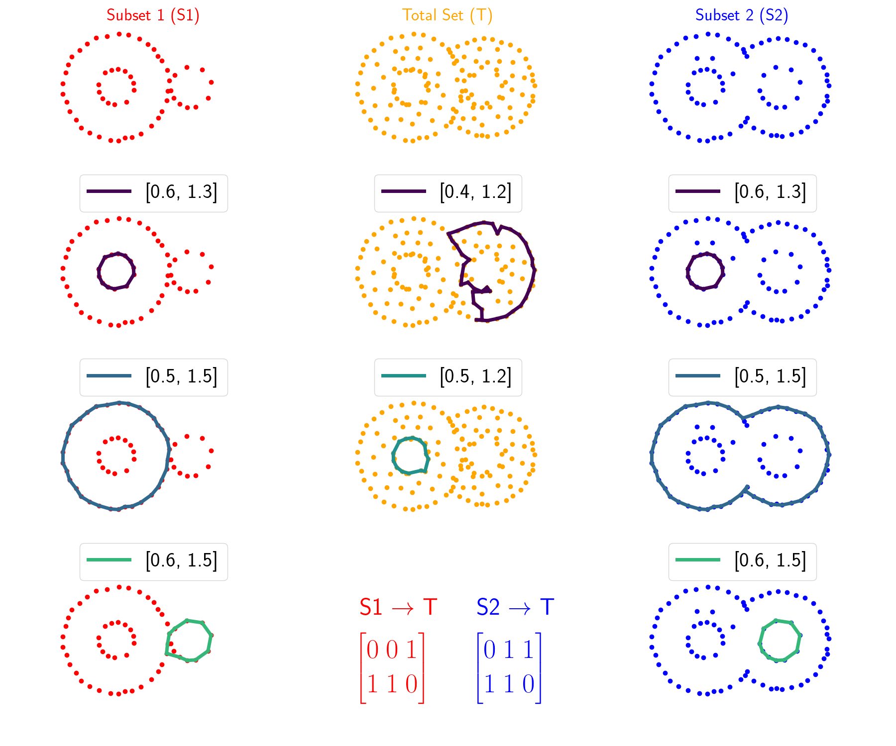
Figure 1: On the top, the point clouds $S_{1}\xhookrightarrow{}T\xhookleftarrow{}S_{2}$ are despicted. In the rest of the pictures, representative cycles of the 1-holes associated with each interval of the interval decomposition of $\operatorname{PH}_{1}(\operatorname{VR}(S_{1}))$, $\operatorname{PH}_{1}(\operatorname{VR}(T))$ and $\operatorname{PH}_{1}(\operatorname{VR}(S_{2}))$ respectively. On the bottom, we can also find the matrix associated with the block function induced by the inclusion $S_{i}\xhookrightarrow{}T$ for $i=1,2$.

Example 1

Let $S_{i}$, $i=1,2$, be the subsets of the dataset $T$ depicted at the top of Figure 1. Let $V_{i}=\operatorname{PH}_{1}(\operatorname{VR}(S_{i}))$, $i=1,2$, and $U=\operatorname{PH}_{1}(\operatorname{VR}(T))$ be the corresponding $1$-dimensional persistent homology modules, with their respective barcodes being ${\bf A}_{i}=\{[0.6,1.3],[0.5,1.5],[0.6,1.5]\}$, $i=1,2$, and ${\bf B}=\{[0.4,1.2],[0.5,1.2]\}$. Now, the morphism $f_{1}:V_{1}\to U$ has associated the following $(2,3)$-matrix whose columns and rows are indexed by ${\bf A}_{2}$ and ${\bf B}$ respectively:

$$F=\left[\begin{array}[]{c|ccc}&[0.6,1.3]&[0.5,1.5]&[0.6,1.5]\\ \hline\cr{[0.4,1.2]}&0&0&1\\ {[0.5,1.2]}&1&1&0\end{array}\right]$$

Similarly, the morphism $f_{2}:V_{2}\to U$ has associated the following matrix:

$$G=\left[\begin{array}[]{c|ccc}&[0.6,1.3]&[0.5,1.5]&[0.6,1.5]\\ \hline\cr{[0.4,1.2]}&0&1&1\\ {[0.5,1.2]}&1&1&0\end{array}\right]$$

Using the induced block function, we will see in Example 2 that $f_{1}$ and $f_{2}$ are not isomorphic, although ${\bf A}_{1}={\bf A}_{2}$.

Now, for each interval $I\in{\bf A}$, we define $F_{I}$ as the submatrix of $F$ given by the columns indexed by the set $A_{I}^{+}$. We denote by $\widetilde{F}_{I}$ the Gaussian column reduction of $F_{I}$. This leads to an easy computation for $\mathcal{M}_{f}$ as

$$\mathcal{M}_{f}(I,J)=\begin{cases}1&\mbox{ if the pivot of the last column from }\widetilde{F}_{I}\mbox{ is at row }J,\\ 0&\mbox{ otherwise,}\end{cases}$$

for all $I\in{\bf A}$ and $J\in{\bf B}$. It is easier to think of a block function as an assignment: for $I\in{\bf A}$ we write $I\mapsto J$ if there exists $J\in{\bf B}$ such that $\mathcal{M}_{f}(I,J)=1$ and $I\mapsto\emptyset$ otherwise. To simplify notation, we write $\mathcal{M}_{f}:{\bf A}\rightarrow{\bf B}$ from now on.

Since we assume that there are no repeated intervals, for each $I\in{\bf A}$ there exists at most one interval $J\in{\bf B}$ such that $\mathcal{M}_{f}(I,J)=1$. However, the converse might not hold, as shown in Example 2.

Example 2

This example continues Example 1. First, observe that the Gaussian reductions of $F_{I}$ for $I\in{\bf A}_{1}$ are given by the following matrices

$$\widetilde{F}_{[0.6,1.3]}=\left[\begin{array}[]{c|ccc}&[0.6,1.3]\\ \hline\cr{[0.4,1.2]}&0\\ {[0.5,1.2]}&1\end{array}\right],\hskip 14.22636pt\widetilde{F}_{[0.5,1.5]}=\left[\begin{array}[]{c|ccc}&[0.5,1.5]\\ \hline\cr{[0.4,1.2]}&0\\ {[0.5,1.2]}&1\end{array}\right],$$

$$\widetilde{F}_{[0.6,1.5]}=\left[\begin{array}[]{c|ccc}&[0.6,1.3]&[0.5,1.5]&[0.6,1.5]\\ \hline\cr{[0.4,1.2]}&0&0&1\\ {[0.5,1.2]}&1&0&0\end{array}\right].$$

Then, the block function $\mathcal{M}_{f_{1}}$ is given by the assignments

$$[0.6,1.3]\mapsto[0.5,1.2]\,,\hskip 8.5359pt[0.5,1.5]\mapsto[0.5,1.2]\,,\hskip 8.5359pt[0.6,1.5]\mapsto[0.4,1.2]\,.$$

Here notice that both intervals $[0.6,1.3]$ and $[0.5,1.4]$ are nested and are sent to the same interval $[0.5,1.2]$. On the other hand, the matrices $\widetilde{G}_{I}$ for $I\in{\bf A}_{2}$ obtained after performing Gaussian eliminations are

$$\widetilde{G}_{[0.6,1.3]}=\left[\begin{array}[]{c|ccc}&[0.6,1.3]\\ \hline\cr{[0.4,1.2]}&0\\ {[0.5,1.2]}&1\end{array}\right],\hskip 14.22636pt\widetilde{G}_{[0.5,1.5]}=\left[\begin{array}[]{c|ccc}&[0.5,1.5]\\ \hline\cr{[0.4,1.2]}&1\\ {[0.5,1.2]}&1\end{array}\right],$$

$$\widetilde{G}_{[0.6,1.5]}=\left[\begin{array}[]{c|ccc}&[0.6,1.3]&[0.5,1.5]&[0.6,1.5]\\ \hline\cr{[0.4,1.2]}&0&1&0\\ {[0.5,1.2]}&1&0&0\end{array}\right]$$

From $\widetilde{G}_{[0.6,1.5]}$ we deduce that $[0.6,1.5]$ is sent to the empty set. Altogether, the resulting block function $\mathcal{M}_{f_{2}}$ is given by the assignments

$$[0.6,1.3]\mapsto[0.5,1.2]\,,\hskip 8.5359pt[0.5,1.5]\mapsto[0.5,1.2]\,,\hskip 8.5359pt[0.6,1.5]\mapsto\emptyset\,.$$

In particular, since $\mathcal{M}_{f_{1}}$ and $\mathcal{M}_{f_{2}}$ are different, the morphisms $f_{1}$ and $f_{2}$ are not isomorphic, since block functions are invariant under isomorphism as proven in [7].

3 Topological Quality of Training Data

Starting from a point cloud $Y\subset\mathbb{R}^{n}$ (the input dataset), in this section we provide a quantitative method to compare the topological quality of subsets of $Y$. We will show experimentally in Section 4 that our measure serves for explaining why some training datasets will lead to worse performance than others.

Given two subsets $X$ and $X^{\prime}$ of the input dataset $Y$, we assume that the block functions $\mathcal{M}_{f}$ and $\mathcal{M}_{g}$ are computed for $f$ and $g$ being morphisms between persistence modules induced by the inclusions $X\xhookrightarrow{}Y$ and $X^{\prime}\xhookrightarrow{}Y$, respectively. We can state the following definition.

Definition 1

Let $X$ be a subset of the input dataset $Y$ and let $\mathcal{M}_{f}$ be the block function induced by the inclusion $X\xhookrightarrow{}Y$. We define the $k$-dimensional topological quality of $X$ with respect to $Y$ as the number

$$\operatorname{TQ}_{k}(X,Y)=\#\{J\in\operatorname{B}(H_{k}(\operatorname{VR}(Y))\ |\ \mathcal{M}_{f}(\cdot,J)\neq 0\}\,.$$

Let $X$ and $X^{\prime}$ be two subsets of the input dataset $Y$. We say that $X$ has better $k$-dimensional topological quality than $X^{\prime}$ with respect to $Y$ if $\operatorname{TQ}_{k}(X,Y)>\operatorname{TQ}_{K}(X^{\prime},Y)$.

We have the following immediate results.

Lemma 1

Let $X$ be a subset of the input dataset $Y$ and let $\mathcal{M}_{f}:\operatorname{B}(V)\to\operatorname{B}(U)$ be the block function induced by the inclusion $X\xhookrightarrow{}Y$, where $V=\operatorname{PH}_{k}(\operatorname{VR}(X))$ and $U=\operatorname{PH}_{k}(\operatorname{VR}(Y))$.

1. Subset size. Measuring the $0$-dimensional topological quality of $X$ is equivalent to counting its number of points.

2. Partial matching bound. The number of matchings of any partial matching between intervals of $\operatorname{B}(V)$ and $\operatorname{B}(U)$ obtained from $\mathcal{M}_{f}$ is $\operatorname{TQ}_{k}(X,Y)$.

3. Well-definedness. If $V\simeq\operatorname{PH}_{k}(\operatorname{VR}(X^{\prime}))$ for $X^{\prime}\xhookrightarrow{}Y$ then $\operatorname{TQ}_{k}(X,Y)=\operatorname{TQ}_{k}(X^{\prime},Y)$.

Proof

Let $V=\operatorname{PH}_{k}(\operatorname{VR}(X))$, $V^{\prime}=\operatorname{PH}_{k}(\operatorname{VR}(X^{\prime}))$ and $U=\operatorname{PH}_{k}(\operatorname{VR}(Y))$.
a)  This is proven in Subsection 3.1: if $k=0$, then $\operatorname{TQ}_{0}(X,Y)$ is simply $\#X$.
b)  In [7], the authors noticed that there are different ways to define a partial matching, induced by $\mathcal{M}_{f}$, between intervals of $\operatorname{B}(U)$ and $\operatorname{B}(V)$. Nevertheless, all the partial matchings that can be obtained from $\mathcal{M}_{f}$ have $\operatorname{TQ}_{k}(X,Y)$ number of matchings.
c)  Let $f:V\to U$ and $g:V^{\prime}\to U$ be induced by the inclusions $X\xhookrightarrow{}Y$ and $X^{\prime}\xhookrightarrow{}Y$ respectively. If $f\simeq g$ then $\mathcal{M}_{f}=\mathcal{M}_{g}$ so $\operatorname{TQ}_{k}(X,Y)=\operatorname{TQ}_{k}(X^{\prime},Y)$ as claimed. ∎

Notice that the converse of the last statement of Lemma 1 is not true in general. That is, two subsets $X$ and $X^{\prime}$ can have the same $k$-dimensional topological quality with respect to $Y$ but $f$ and $g$ are not necessarily isomorphic. In the following example, we continue Example 2 and compute the $1$-dimensional topological quality of the subsets $S_{i}$ for $i=1,2$.

Example 3

From the block functions computed, we obtain that $\operatorname{TQ}_{1}(S_{1},T)=2$ and $\operatorname{TQ}_{1}(S_{2},T)=1$, so we claim that the subset $S_{1}$ has better $1$-topological quality than the subset $S_{2}$ with respect to $T$.

3.1 Embedding of the $0$-dimensional barcode

In this subsection, we show that the inclusion $X\hookrightarrow Y$ implies that the block function $\mathcal{M}_{f}$ induces an embedding of barcodes ${\bf A}\hookrightarrow{\bf B}$ for the $0$-dimensional persistent homology.

Proposition 1

Let $f:V\rightarrow U$ be induced by the inclusion $X\hookrightarrow Y$, where $V=\operatorname{PH}_{0}(\operatorname{VR}(X))$ and $U=\operatorname{PH}_{0}(\operatorname{VR}(Y))$. Let ${\bf A}=\operatorname{B}(V)$ and ${\bf B}=\operatorname{B}(U)$. Then $\mathcal{M}_{f}$ defines an embedding of barcodes ${\bf A}\hookrightarrow{\bf B}$.

Proof

First of all, both barcodes ${\bf A}$ and ${\bf B}$ have an interval decomposition with all intervals starting at value $0$. This implies that there are no nested intervals since if two intervals $[a,b],[c,d]$ are nested, then the strict inequality $a<c$ must hold since $a=c=0$. Thus, we can rely on Theorem 5.5 from [7] and deduce that for each interval $J\in{\bf B}$, there exists at most one interval $I\in{\bf A}$ such that $\mathcal{M}_{f}(I,J)=1$. Besides, since there are no repeated intervals, using the block function bound stated at the start of subsection 2.2 we obtain that for each $I\in{\bf A}$ there exists at most one interval $J\in{\bf B}$ such that $\mathcal{M}_{f}(I,J)=1$.

We claim that, for each $I\in{\bf A}$, there is always $J\in{\bf B}$ such that $\mathcal{M}_{f}(I,J)=1$. First, we notice another consequence of not having nested intervals: the barcode ${\bf A}$ is a totally ordered set, where $[0,a]\leq[0,b]$ if and only if $a\leq b$. In particular, given $I\in{\bf A}$, we might write ${\bf A}^{+}_{I}=\{L\in{\bf A}\,|\,L\leq I\}$. Denote by $F$ the associated matrix with $f$ and let $\widetilde{F}$ be its reduced column form. By the previous observation, the matrix $\widetilde{F}_{I}$ is the submatrix of $\widetilde{F}$ obtained by taking all columns that go before and including the column labeled by $I$. Thus, using the definition of $\mathcal{M}_{f}$ from Subsection 2.2, our claim follows if all columns from $\widetilde{F}$ are non-trivial; i.e. ${\rm rank}(F)=\#{\bf A}$. Now, the matrix $F$ is also associated to $f_{0}:\operatorname{H}_{0}(\operatorname{VR}_{0}(X))\rightarrow\operatorname{H}_{0}(\operatorname{VR}_{0}(Y))$ (taking a particular choice of bases). However, observe that the linear morphism $f_{0}$ is given by the injection $\operatorname{VR}_{0}(X)=X\hookrightarrow Y=\operatorname{VR}_{0}(Y)$ and so ${\rm rank}(F)=\#X=\#{\bf A}$ as claimed. ∎

4 Experiments

The code used for our experiments comes from an implementation that works for a more general case. The code is a Python implementation that uses GUDHI [8] for the Vietoris-Rips computation and PHAT for computing persistent homology, which leads to both barcodes and representative cycles. As we are using PHAT [1], our experiments are conducted taking the field $\mathbb{Z}_{2}$. Given an inclusion of finite subsets from $\mathbb{R}^{n}$, $X\xhookrightarrow{}Y$, we consider the induced morphism $f:\operatorname{PH}_{k}(\operatorname{VR}(X))\rightarrow\operatorname{PH}_{k}(\operatorname{VR}(Y))$. The matrix $F$ associated with $f$ and the induced block function $\mathcal{M}_{f}$ are computed as explained in Subsection 2.2. The code will be publicly available in a GitHub repository after the revision process.

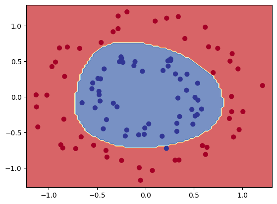
Figure 2: The input dataset $Y$ considered in Subsection 4.1 consists of a finite set of red and blue points in $\mathbb{R}^{2}$. Then, the points of $\mathbb{R}^{2}$ are divided into two regions (red and blue) predicted by a classifier trained with the dataset $Y$.

4.1 Experiment 1

For this first experiment, we consider the input dataset $Y$ depicted in Figure 2 which consists of a set of points divided into two classes labeled red and blue, $Y=Y^{\operatorname{red}}\cup Y^{\operatorname{blue}}$. The classifier considered is a feed-forward neural network with $2\times 3\times 2$ nodes and one hidden layer, with the hyperbolic tangent function as the activation function. Firstly, we trained the neural network $1000$ epochs with the input dataset $Y$ using stochastic gradient descent. The regions predicted are shown in Figure 2.

Figure 3: On the top, the three subsets $S_{1}$, $S_{2}$ and $S_{3}$ considered in Subsection 4.1 are displayed. All of them are composed of $5$ blue points and $5$ red points. On the bottom, we can see the regions predicted by the classifier trained $1000$ epochs with each subset considered using stochastic gradient descent.

Now, we consider three subsets ($S_{i}=S_{i}^{\operatorname{red}}\cup S_{i}^{\operatorname{blue}}$, for $i=1,2,3$) of the input dataset $Y$. These subsets are pictured at the top of Figure 3. Then, we train the classifier for each subset $S_{i}$, $i=1,2,3$. The regions predicted by the classifier are depicted at the bottom of Figure 3. As we can observe, the regions for the subset $S_{3}$ are similar to the ones pictured in Figure 2 for the input dataset $Y$, as the red region wraps around the blue region, unlike the regions for the subsets $S_{i}$, for $i=1,2$. Let us see that such behavior is also reflected by the block functions $\mathcal{M}_{f^{x}_{i}}$ induced by the morphisms $f^{x}_{i}:\operatorname{PH}_{1}(\operatorname{VR}(S^{x}_{i}))\to\operatorname{PH}_{1}(\operatorname{VR}(Y))$ for $x\in\{\operatorname{red},\operatorname{blue}\}$ and $i=1,2,3$.

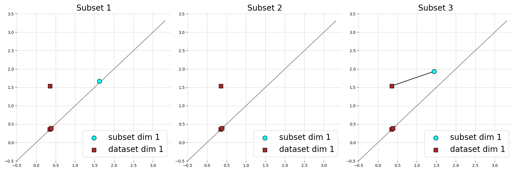
Figure 4: A graphical illustration of the block function $\mathcal{M}_{f^{\operatorname{red}}_{i}}$, for $i=1,2,3$. Cyan-circled points belong to the persistence diagram of ${\bf B}(\operatorname{PH}_{1}(\operatorname{VR}(S_{i}^{\operatorname{red}})))$, for $i=1,2,3$, and brown-squared points belong to the persistence diagram of ${\bf B}(\operatorname{PH}_{1}(\operatorname{VR}(Y^{\operatorname{red}})))$.

A graphical representation of the block function $\mathcal{M}_{f^{\operatorname{red}}_{i}}$ induced by the morphism $f^{\operatorname{red}}_{i}:\operatorname{PH}_{1}(\operatorname{VR}(S_{i}^{\operatorname{red}}))\to\operatorname{PH}_{1}(\operatorname{VR}(Y^{\operatorname{red}}))$, for $i=1,2,3$, is provided in Figure 4, where the persistence diagram of the barcode $\operatorname{B}(\operatorname{PH}_{1}(\operatorname{VR}(S^{\operatorname{red}}_{i})))$, for $i=1,2,3$, is pictured. We can observe that there is only a matching, induced by the inclusion $S_{3}^{\operatorname{red}}\xhookrightarrow{}Y$. This way we have:

$$\operatorname{TQ}_{1}(S^{\operatorname{red}}_{1},Y)=0=\operatorname{TQ}_{1}(S^{\operatorname{red}}_{2},Y)\;\mbox{ and }\;\operatorname{TQ}_{1}(S^{\operatorname{red}}_{3},Y)=1\,.$$

Therefore, the subset $S^{\operatorname{red}}_{3}$ has better 1-dimensional topological quality with respect to the dataset $Y$ than the subsets $S^{\operatorname{red}}_{1}$ and $S^{\operatorname{red}}_{2}$, supporting the idea that the neural network trained with the dataset $S^{\operatorname{red}}_{3}$ captures better the fact that the red points belong to a region that encloses the region containing the blue points. It is worth noticing that the matching induced for Subset 3 could not have been deduced by standard techniques, such as computing the bottleneck distance, since the matched points are closer to the diagonal than to each other.

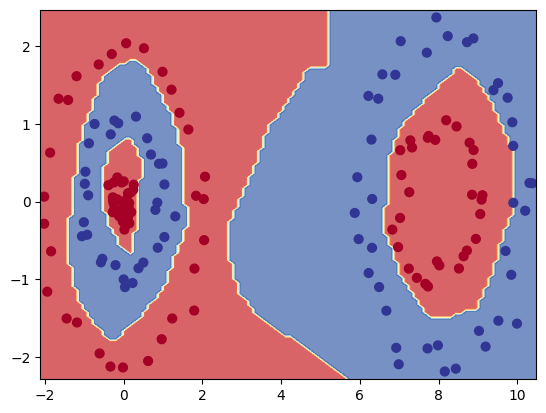
Figure 5: Dataset $Z$ considered in Subsection 4.2. The points of $\mathbb{R}^{2}$ are divided into two zones (red and blue). The input dataset $Z$ with red and blue points samples the two zones. The dataset is composed of $70$ red points and $80$ blue points.

4.2 Experiment 2

Similarly to Experiment 1, in this experiment, we consider that the points of the plane $\mathbb{R}^{2}$ are divided into two classes (red and blue) as pictured in Figure 5. The input dataset considered is denoted as $Z$ and pictured in Figure 5. We take two subsets ($S_{i}=S_{i}^{\operatorname{red}}\cup S_{i}^{\operatorname{blue}}$, for $i=1,2$) of the input dataset $Z$ which we indicate in Figure 6. The classifier considered in this experiment is a feed-forward neural network with $2\times 32\times 32\times 16\times 2$ nodes. It was trained $2000$ epochs using RMSProp and ReLu activation functions. As we can observe, the regions predicted by the classifier using subset $S_{1}$ are much closer to those from Figure 5 than the regions predicted using $S_{2}$. We obtained the following quantities for the red class:

$$\operatorname{TQ}_{1}(S_{1}^{\operatorname{red}},Y)=4\,,\mbox{ and }\operatorname{TQ}_{1}(S_{2}^{\operatorname{red}},Y)=3\,.$$

For the blue class, we obtained that both subsets have the same $1$-dimensional topological quality: $\operatorname{TQ}_{1}(S_{1}^{\operatorname{blue}},Y)=\operatorname{TQ}_{1}(S_{2}^{\operatorname{blue}},Y)=2\,.$ We depict the corresponding block functions in Figure 7. We then can corroborate that the $1$-dimensional topological quality of the subset $S_{1}$ is better than the quality of $S_{2}$ as expected.

Figure 6: Subsets $S_{1}$ and $S_{2}$ are plotted at the top, while at the bottom we depict their corresponding prediction regions. Both subsets are composed of $40$ red points and $50$ blue points.

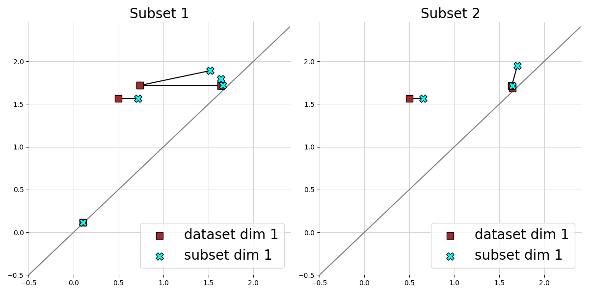
Figure 7: Block functions $\mathcal{M}_{f^{\operatorname{red}}_{i}}$, for $i=1,2$. For pictorial clarity, we have omitted the intervals that are not matched by $\mathcal{M}_{f_{i}^{\operatorname{red}}}$.

5 Conclusion and future works

In this paper, we have provided a novel definition of data quality based on $k$-dimensional topological features to measure the quality of a training subset relative to the entire input dataset. Theoretical results support that the proposed definition is well-stated, measuring the size of the subset in the $0$-dimensional case and is coherent with previous related definitions such as partial matchings. The experiments made show that topological quality is a measure that can be used to provide an explanation of why the chosen training subset will lead to poor performance.

As a future work, an interesting research topic is to adapt our method to be robust to outliers in this context and to optimize our code to be used on large datasets.

References

- [1] Bauer, U., Kerber, M., Reininghaus, J., Wagner, H.: Phat – persistent homology algorithms toolbox. Journal of Symbolic Computation 78, 76–90 (2017). https://doi.org/10.1016/j.jsc.2016.03.008
- [2] Bender, E.M., Gebru, T., McMillan-Major, A., Shmitchell, S.: On the dangers of stochastic parrots: Can language models be too big? In: Proc of the 2021 ACM Conf on Fairness, Accountability, and Transparency. p. 610–623 (2021). https://doi.org/10.1145/3442188.3445922
- [3] Black, A., Nederpelt, P.v.: Dimensions of data quality (ddq). DAMA NL Foundation (2020), https://dama-nl.org/
- [4] Carlsson, G., Vejdemo-Johansson, M.: Topological Data Analysis with Applications. Cambridge University Press (2021). https://doi.org/10.1017/9781108975704
- [5] Choo, J., Liu, S.: Visual analytics for explainable deep learning. IEEE Computer Graphics and Applications 38(4), 84–92 (2018). https://doi.org/10.1109/MCG.2018.042731661
- [6] Edelsbrunner, H., Harer, J.: Computational Topology: An Introduction. Applied Mathematics, American Mathematical Society (2010)
- [7] Gonzalez-Diaz, R., Soriano-Trigueros, M., Torras-Casas, A.: Partial matchings induced by morphisms between persistence modules. Computational Geometry 112, 101985 (2023). https://doi.org/10.1016/j.comgeo.2023.101985
- [8] Maria, C., Dlotko, P., Rouvreau, V., Glisse, M.: Rips complex. In: GUDHI User and Reference Manual. GUDHI Editorial Board, 3.8.0 edn. (2023), https://gudhi.inria.fr/doc/3.8.0/group__rips__complex.html
- [9] Mehrabi, N., Morstatter, F., Saxena, N., Lerman, K., Galstyan, A.: A survey on bias and fairness in machine learning. ACM Comput. Surv. 54(6) (jul 2021). https://doi.org/10.1145/3457607
- [10] Oudot, S.: Persistence Theory - From Quiver Representations to Data Analysis. Cambridge University Press (2015)
- [11] Saeed, W., Omlin, C.: Explainable ai (xai): A systematic meta-survey of current challenges and future opportunities. Knowledge-Based Systems 263, 110273 (2023). https://doi.org/10.1016/j.knosys.2023.110273